Metadetection Weak Lensing for the Vera C. Rubin Observatory

Abstract

Forthcoming astronomical imaging surveys will use weak gravitational lensing shear as a primary probe to study dark energy, with accuracy requirements at the 0.1% level. We present an implementation of the metadetection shear measurement algorithm for use with the Vera C. Rubin Observatory Legacy Survey of Space and Time (LSST). This new code works with the data products produced by the LSST Science Pipelines, and uses the pipeline algorithms when possible. We tested the code using a new set of simulations designed to mimic LSST imaging data. The simulated images contained semi-realistic galaxies, stars with representative distributions of magnitudes and galactic spatial density, cosmic rays, bad CCD columns and spatially variable point spread functions. Bright stars were saturated and simulated “bleed trails” were drawn. Problem areas were interpolated, and the images were coadded into small cells, excluding images not fully covering the cell to guarantee a continuous point spread function. In all our tests the measured shear was accurate within the LSST requirements.

1 Introduction

New astronomical imaging surveys coming online in the next few years will use weak gravitational lensing shear as a primary probe to study dark energy. These “stage IV” dark energy experiments, the Rubin Observatory Legacy Survey of Space and Time (LSST, Ivezić et al., 2008), the Euclid mission (Laureijs et al., 2011) and surveys with the Nancy Grace Roman Space Telescope (Spergel et al., 2015; Akeson et al., 2019) require shear measurement methods that are accurate to a few tenths of a percent (Massey et al., 2013; Mandelbaum et al., 2018), and implementations of those algorithms that work with the data products of each survey.

A number of promising shear measurement techniques have been developed over the last few years. The metadetection shear measurement method (Sheldon et al., 2020) has better than 0.1% accuracy for noisy data, overlapping, or “blended”, galaxy images and a constant applied shear (Sheldon et al., 2020; Hoekstra et al., 2021; Hoekstra, 2021). At the time of writing, other recently developed methods provide similar accuracy for isolated galaxy images (Bernstein et al., 2016; Li & Mandelbaum, 2022) but require further percent level corrections from simulations to account for blending effects (Sheldon et al., 2020; Li & Mandelbaum, 2022).

Real astronomical images contain additional features that must be addressed in order to obtain accurate shear measurements. A typical image may be expected to contain, among other features, cosmic rays, bad CCD columns, saturation, Milky Way stars (which are not lensed significantly) and star “bleed trails”. For computational efficiency the images may be remapped and summed into aggregates, or “coadded”, which can result in spatially correlated image noise.

An accurate shear measurement method must be unbiased (up to higher order shear effects) in the presence of these image features. That is, if the input data are well characterized in terms of flux calibration, astrometry, background determination, noise properties, and PSF, and if problematic features are identified and masked, the technique should provide an accurate shear measurement.

In actual analyses on real data, errors in the calibration and characterization of the data may contribute significantly to the systematic error in the shear measurement. For an accurate shear measurement, the ultimate limit may be the characterization of the data, not the method itself.

In this work we demonstrate that the metadetection technique can accurately calibrate shear estimates in such featureful, but well-characterized data. We simulate images containing galaxies, stars with a realistic galactic density distribution, spatially variable PSF, and proxies for the above image artifacts (see §2), which we interpolate, or “warp”, onto a common reference frame and sum into overlapping coadds (see §3). Each feature was switched on or off independently to control potential sources of error. We simulate the expected data products produced by the LSST Science Pipelines (Bosch et al., 2019, 2017), and use a new metadetection code designed specifically to work with Science Pipeline data structures and algorithms. We describe metadetection in §4, and the results in §6.

2 Simulation Features

The basic simulation was similar to that created for (Sheldon et al., 2020). We added additional features such as image artifacts, cosmic rays, stars, and saturated stars which we will describe in the following sections. All images were rendered using the GALSIM python package. For this work, we used the newly written simulation package descwl-shear-sims version 0.4.2.

As our basic data product, we simulated the calibrated exposure images produced by the LSST Science Pipelines version w_2021_32. This data is stored in an Exposure data structure, which carries a calibrated, background subtracted image, along with an estimated noise variance image plane, world coordinate system transformation (WCS) and position-dependent PSF model. Problem areas associated with saturation, cosmic rays, and bad columns are marked as separate bits in an integer bit mask image plane.

Other than simple, constant background estimation errors, which were easy to implement and test (see §2.9), we did not simulate scenarios in which the input data were miscalibrated. For example we did not test the consequences of inaccurate PSF models, noise estimates or photometric calibrations. Our motivation was to test the performance of metadetection using well-characterized data. It may be necessary to propagate or simulate the effects of miscalibrated data in order to characterize the final shear calibration in real data analyses.

Importantly, our approach to simulations in this work was not to simulate every possible effect in detail. Such simulations, like the Data Challenge 2 (DC2) simulations (Abolfathi et al., 2021) for example, while physically more realistic than our approach here, are exceedingly complex to analyze and can be computationally much more expensive than the approach we took in this work. Instead, we approached our simulation analysis as a series of detailed numerical experiments where single features are changed one at a time. This level of control combined with reasonably fast codes was needed for us to reach our goal of constraining the bias in our algorithms with a precision better than the LSST requirements of 0.002 (see §6.1). For example, for the tests shown in §6.6, we simulated a total of 41,600 square degrees, providing constraints well within our requirements at 99.7% confidence. On the other hand, the simulated area in DC2 is about 300 square degrees, which would provide constraints only at the percent level. Furthermore, using the existing DC2 simulation does not allow control over the simulation features, so that in general it would not be possible to isolate the source of shear measurement biases. Future work building on our approach here and carefully examining one feature at a time will be essential for delivering accurate shear measurements for LSST.

2.1 Image Filters and Noise

We used the WeakLensingDeblending package (Sanchez et al., 2021) to predict the image noise according to the Rubin Observatory/LSST filter being simulated. In all simulation runs we used noise $n$ for the final 10 year coadd. If $N$ simulated images were created, representing data from individual exposures to be coadded, we re-scaled the noise appropriately, such that the noise in each image was $n*\sqrt{N}$.

We did not simulate a realistic background and background noise for each image (see §2.9). We instead used Gaussian noise to approximate the Poisson noise that would remain in each image after background subtraction. After drawing all image features and adding noise, we re-scaled the images to a common zero point of 30 before coadding.

We did not include the Poisson noise from objects. This was mainly an optimization, as it is inefficient to simulate the large number of photons from bright objects. We have tested metacalibration with object Poisson noise for faint, sky noise dominated objects, but not brighter objects, which we leave to future work.

2.2 Image World Coordinate System, Rotations and Dithers

Each image was simulated as a tangent plane projection of the sky onto the image frame with the expected LSST camera pixel scale of 0.2 arcseconds (Ivezić et al., 2008). The world coordinate system (WCS) transformation between sky and pixel coordinates was represented as a GALSIM tangent plane WCS object (TanWCS). Each simulated WCS transformation had a random rotation applied, in order to mock up the camera rotations used by LSSTCam (Ivezić et al., 2008). The center of each image was shifted, or “dithered”, randomly in two dimensions relative to the center of the desired coadded image. For efficiency, we used dithers that were unrealistically small, within two pixels, to minimize portions of the image that would not overlap the final coadd. We created images with sizes just large enough that the rotated image, after dithers, would have no edge crossing the coadd region, again to avoid waste: coadding an image with an edge produces a discontinuous PSF in the final coadd, so such images would be discarded.

The simulated image was copied into an Exposure data structure with an equivalent LSST Science Pipelines tangent plane SkyWCS.

2.3 Point Spread Function

For our basic PSF model we used a Moffat profile (Moffat, 1969) with shape parameter $\beta=2.5$ and full width at half maximum (FWHM) of 0.8 arcseconds.

We also generated spatially variable PSF models, varying both the ellipticity and size across the image, using the methods described in Appendix A of Sheldon et al. (2020) based on work by Heymans et al. (2012). Heymans et al. (2012) used images with high stellar density to fit a von Kármán  model of atmospheric turbulence to the PSF variation. Sheldon et al. (2020) used this model, with a modification to reduce unrealistically large power below 1”, to generate realizations of spatially variable PSFs using Gaussian random fields. The PSF model was again a Moffat profile with shape parameter $\beta=2.5$ but with variable size and shape.

In Sheldon et al. (2020) this approximate variable PSF model was compared to detailed atmospheric and optics simulations for the Dark Energy Survey (DES), and the variation was tuned to exceed the expectations of real data by a factor of 10. We used the same models for this work, but with a variation tuned to match, rather than exceed, expectations for DES. The level of variations for DES at the Cerro Tololo site should be a rough approximation to the variations at the nearby Rubin observatory at Cerro Pachón. The median FWHM of the generated PSFs was 0.8 arcseconds for all bands. We also ran simulations with larger than expected variations in order to test the accuracy of the PSF coadd under extreme, unrealistic conditions.

We did not include other sources of spatial PSF variation such as effects from the optical surfaces in the telescope. We also did not include any chromaticity in the PSF (Plazas & Bernstein, 2012; Meyers & Burchat, 2015; Kamath et al., 2020) or galaxy color gradients that complicate the PSF correction. We leave such considerations to future work.

2.4 Stars

We simulated stars using fluxes and Milky Way densities sampled from the LSST DESC Data Challenge Two (DC2) simulation catalogs (Abolfathi et al., 2021). For each simulated field we sampled randomly, with replacement, from the map of stellar density used to generate DC2, rejecting densities higher than 100 per square arcminute. This density represents the total number of stars drawn, not the number detected. The multi-band flux for each star was sampled with replacement from the DC2 star catalog. We modeled each star as a point source convolved with the point spread function (see §2.3). Stars were allowed to saturate and have an associated bleed trail (see §2.5).

2.5 Image Saturation, Star Masking and Star Bleed Trails

The value in each pixel was artificially limited in order to simulate saturation, saturated pixels were marked with an appropriate flag in the integer bitmask image of the Exposure, and finally the variance for those pixels was set to infinity. Non-linear detector response was not simulated.

Saturated stars were over-drawn with a simulated bleed trail image, taken from a set of pre-generated templates identified in images of bright stars created using the DC2 code. For each saturated star in our simulation, we found a star in the template set with closely matched flux in the filter of interest and drew the associated bleed image directly over the star image with a value set to the saturation level. The bleed pixels were marked with the appropriate flag in the bitmask.

Before performing PSF deconvolution on the coadds, we further masked saturated stars with a circle that covered the star out to the radius where the profile reached the noise level. Note in real data such a mask would need to be determined algorithmically. This region was set to zero in the image and marked appropriately in the bitmask. This mask does not necessarily cover the bleed trail completely, although the trails were interpolated in the original images before warping (see §3). We find that these unmasked trails do not cause a shear bias, which we attribute to the camera rotations that randomize the direction of the trail on the sky.

Masks with sharp features can cause ringing in the FFTs used by the metadetection algorithm. Each star mask is like a circular “tophat”, which will have a sharp feature where it intersects an object in the image. We mitigated this effect using the apodization procedure described in Becker et al. (in prep.). We extended the star mask by 16 pixels and forced the mask to smoothly transition from zero in the interior of the circle to unity at the expanded edge. The transition region was parameterized using the cumulative integral of a triweight kernel. This kernel is a function of two parameters, $m$ and $h$, and is defined for a point $x$ with quantity $y=(x-m)/h$ as

$$K(x,m,h)=\begin{cases}0&y<-3\\ (-5y^{7}/69984\\ +7y^{5}/2592\\ -35y^{3}/864&-3\leq y\leq 3\\ +35y/96\\ +1/2)\\ 1&y>3\end{cases}$$ (1)

The kernel goes from zero to unity over a span of $6h$, centered on $m$. The general logic is to set $h$ large enough that the variation across the edge is slower than the variation given by the PSF profile, but not so large that area in the image is wasted unnecessarily. We set $h$ to 1.5 pixels and set $m+3h$ to the radius of the star mask hole so that the mask reaches unity at its nominal size.

2.6 Cosmic Rays & Bad Columns

We followed Becker et al. (in prep.) in generating bad column and cosmic ray artifacts. For cosmic rays, we selected a random location on the image, a random angle, and a random length between 10 and 30 pixels. We then flagged pixels along this line as having been hit by a cosmic ray, making sure that pixels that touch only along corners have the pixels directly adjacent to them flagged as well. We set a cosmic ray bit in the bitmask for interpolation later and set the image value to NaN to ensure that no flagged pixels are inadvertently used in the final shear estimates.

We generated bad column masks using a slightly modified Monte Carlo generator from Becker et al. (in prep.). Each bad column was a single pixel wide, positioned randomly on the image. We also added gaps at random to the bad columns to simulate bad columns which do not span the full CCD. We generated a single bad column for each image.

The LSST will generate hundreds of exposures overlapping each location in the survey. It is likely that detection and lensing measurements will be carried out on coadded images, with artifacts interpolated on the original data before being warped and added. The aggregate number of artifacts will be large, but the impact of each artifact will be relatively small. It was not computationally feasible to simulate such a large number of individual images to be coadded in order to test the effect of artifacts in a realistic way. Rather we simulated a smaller number of images per band, typically 1 but up to 10 (see §6.3), with the noise scaled so that the final coadd noise matched LSST 10 year data. Thus, relative to expected LSST data the impact of each artifact on the coadd was large but the aggregate number of artifacts was small.

2.7 Galaxies

We used the WeakLensingDeblending package to generate galaxy models (Sanchez et al., 2021). These elliptical, color galaxy models have bulge, disk and AGN components. The components have the same morphology in each band. This catalog has a raw density of $\sim 240$ galaxies per square arcminute, and an effective $i$-band ab magnitude limit of $\sim 27$. Rather than use the WeakLensingDeblending package to draw the models in the image, we drew the models using Galsim in our code in order to use our own PSF models (see §2.3), and to allow for more efficient drawing.

We also performed simulation runs with single component, round exponential galaxies with fixed flux and size. These models are useful for shear recovery tests that do not require a realistic galaxy population, but benefit from using low shape noise shear tracers. We also used these models for relatively fast shear tests after major code changes, as further verification after the faster unit tests had passed.

2.8 Layouts

We ran tests with both random and gridded galaxy layouts. The random layout was used for the realistic galaxy population, with a density of objects that reflected the expected density of galaxies as defined in the WeakLensingDeblending package. The grid was used with the simple, round exponential galaxies to facilitate relatively fast shear recovery tests. The grid was square, with spacing designed to avoid overlap between adjacent galaxies, and thus avoid blending effects.

See §2.7 for descriptions of each galaxy model type.

2.9 Image Background

We added a constant to the images to approximate errors in the background determination. The motivation was to test if background estimation errors in individual images can be corrected in the final coadd (see §4.2 and §6.4).

We ran tests with both positive and negative backgrounds, and a wide range of absolute values, and got consistent results. For the results presented below, we chose a small negative background, with value of order the image noise level, to simulate a slight over subtraction.

2.10 Overlapping Coadd Cells

Coadds can be used for shear measurement (Armstrong, R., et al., in prep.), with the requirement that the coadded images have a continuous PSF in order to facilitate accurate PSF modeling. Images that have an edge in the coadd region must be rejected. Smaller coadds result in fewer images being rejected, but very small coadds would complicate object identification and deblending. For LSST, we plan to use relatively small (250x250 pixels) overlapping (50 pixels) coadded regions for shear measurement, which we call “cells” because they are small subregions of the larger “tract” regions defined within the LSST Science Pipelines framework.

Each cell definition has an extra boundary area that overlaps neighboring cells. This extra area provides a buffer that reduces measurement problems that can occur at the image edge. Objects with a measured center inside overlaps are trimmed after the detection phase to avoid duplication.

We ran simulations with and without cells in order to control for issues specific to the cell processing and trimming of objects to non overlapping regions.

2.11 Shear Patterns

We implemented two different types of shear pattern. In one we used a single shear for all images, with constant magnitude and orientation. The second type was a constant magnitude shear, but with random orientation for each image. These two scenarios result in equivalent shear recovery bias when objects are not divided into cells on the sky (see §2.10) but, as we will see in §6.5, a small additional selection bias is introduced for random shears when trimming the detected objects to the unique cell regions. In all cases the simulated shear had magnitude of 0.02.

2.12 Noise Images

The metacalibration procedure involves deconvolution by the PSF, shearing of the image, and reconvolution by a round kernel. This process alters the noise and produces a spurious shear response (Sheldon & Huff, 2017). We can cancel this bias by adding a noise image, with properties that statistically match the real background noise, processed with the orthogonal shear (Sheldon & Huff, 2017; Sheldon et al., 2020).

It is important that these noise images also contain the same correlated noise as the real data. We followed the procedure outlined in Becker et al. (in prep.) to generate the noise images. Namely, because the images are manipulated before coaddition, for example interpolating saturated regions, bad columns, etc., we passed the noise images through these manipulations as well. Furthermore, warping will produce correlated noise, and thus the noise images are generated with the same WCS as the real images, and the same warping is applied.

We stored this noise image in a copy of the image Exposure structure, but replacing the real image data with the noise image.

3 Image and PSF Coaddition

For coaddition, we used the coadding strategy described in Becker et al. (in prep.). We reimplemented that strategy using LSST Science Pipelines algorithms for the various steps in the package descwl_coadd. This work uses version 0.3.0 of descwl_coadd.

For warping the images, we used the Lanczos3 interpolant. The warped images were combined with the AccumulatorMeanStack from lsst.meas.algorithms sub package. We used an inverse variance weighting, based on the median of the variance image plane.

Before warping, we interpolated the simulated artifacts in each image such as cosmic rays, bad columns, and saturated pixels. The interpolation and warping modify the noise properties of the image. Thus, for accurate metacalibration noise corrections (see §2.12) we must also run the noise image through the same procedures. Note stars were masked in the coadds, rather than the input images (see §2.5).

Rather than use the LSST Science Pipelines interpolation codes, we followed Becker et al. (in prep.), performing all interpolation of artifacts and saturated regions using the CloughTocher2DInterpolator from the scipy software package. We used this interpolation because the LSST Science Pipelines cosmic ray interpolation available at the time of writing is intertwined with the detection of cosmic rays, so cannot be run on the noise image.

As shown in Armstrong, R., et al. (in prep.) and Becker et al. (in prep.), creating a PSF image for the coadd requires detailed tracking of the sub-pixel offsets of the individual images in the coadd. For each input image, we generated an image of the PSF at the location of the coadd center in the input image. The coadd image center may fall at an arbitrary sub-pixel offset in the input image, and the PSF was drawn with a matching offset. We then warped these PSF images and coadded them using the same weights as the image data. The off-centering and warping is important so that the PSF includes the same small amount of smearing present in the image interpolation. Not including this offset results in percent level multiplicative shear biases (Armstrong, R., et al., in prep.). Note LSST Science Pipelines provides a PSF coadding code, but at the time of writing it did not offset the PSFs before coadding, so was unsuitable for our purposes. The resulting coadd and PSF coadd data were stored in a new Exposure data structure for use in metadetection.

In figure 1 we show an example color image created from warped $r$, $i$, and $z$ simulated images. Figure 2 shows the corresponding masked images, along with the variance and bitmask planes.

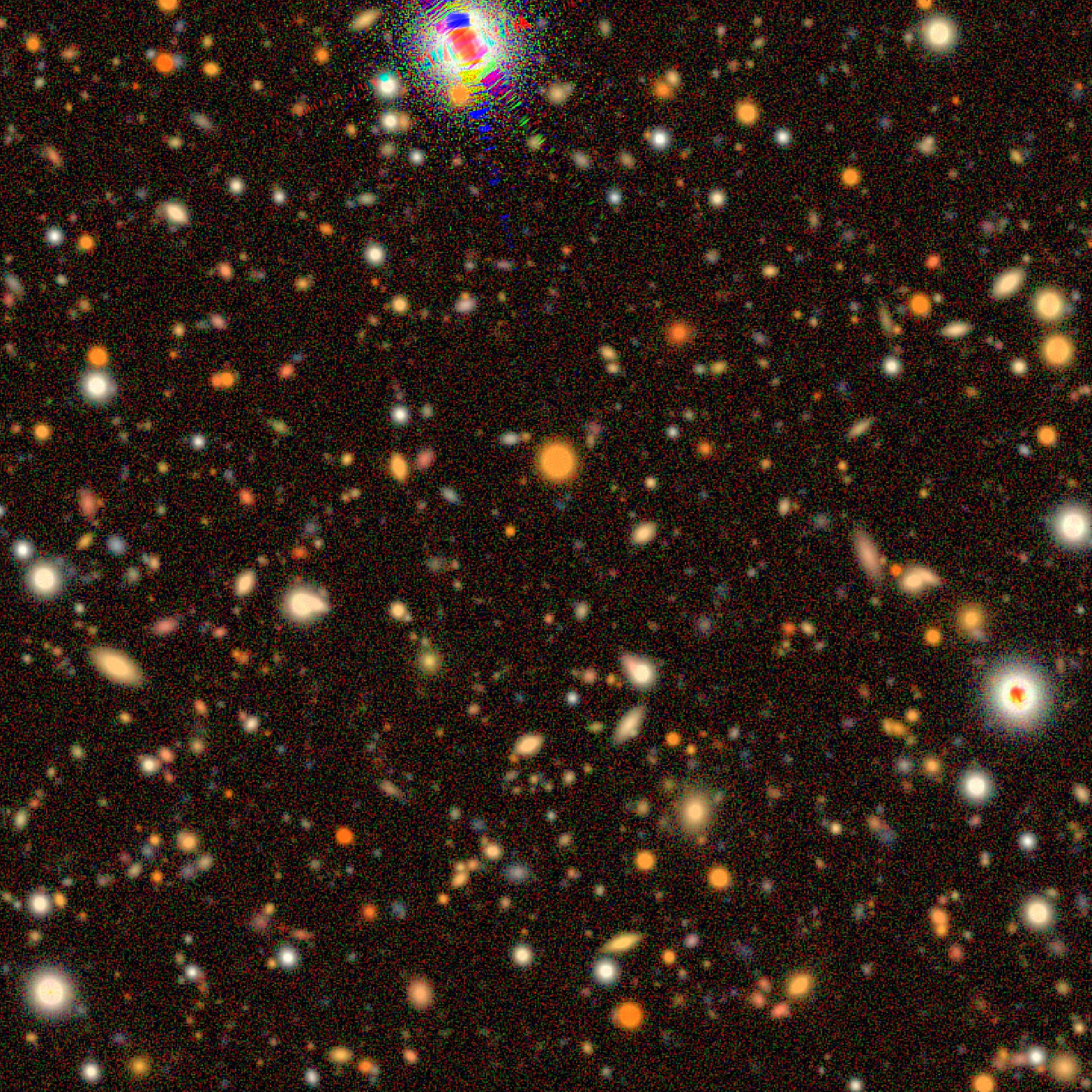
Figure 1: Example simulated image using a single image for each of the $r$, $i$, and $z$ bands, but with noise corresponding to the 10 year LSST coadd data. The images have rotations, dithers and image defects which are interpolated. The images were warped to a common coordinate system. Note the interpolated bleed trails around a bright star in the upper part of the image, appearing at different orientations due to the simulated camera rotations.

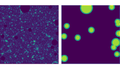
Figure 2: Example masked image corresponding to the $r$ band image used in figure 1, after star masking. The left panel shows the masked image and the right shows the bitmask. The circles represent the star masks applied to each coadd image before PSF deconvolution. The star masks are also marked in the bitmask to facilitate processing near stars. The inner circle in the bitmask is the original mask size and the outer represents the expanded, apodized mask region. In the original images, there are also pixels marked for cosmic rays and bad columns, but these are not retained in the coadd bitmask.

4 Metadetection

For shear inference, we used the metadetection method presented in Sheldon et al. (2020). Metadetection is an extension of the metacalibration method (Huff & Mandelbaum, 2017; Sheldon & Huff, 2017) to include the object identification stage. We call this “detection”, meaning specifically object identification rather than detection of pixels with significant signal. Metadetection mitigates biases due to the shear-dependent nature of the detection process in finite resolution images, biases which are expected to be a few percent for LSST (Sheldon et al., 2020).

Briefly, for metacalibration we assume that the true applied, two-component shear $\boldsymbol{\gamma}$ is small, so that a measured ellipticity $\boldsymbol{e}$ of a galaxy is approximately linear in the shear:

$$\boldsymbol{e} \approx \left.\boldsymbol{e}\right|_{\gamma=0}+\left.\frac{\partial\boldsymbol{e}}{\partial\boldsymbol{\gamma}}\right|_{\gamma=0}\boldsymbol{\gamma}+O(\boldsymbol{\gamma}^{2})$$ (2)

$$\equiv \left.\boldsymbol{e}\right|_{\gamma=0}+\boldsymbol{R}\boldsymbol{\gamma}+O(\boldsymbol{\gamma}^{2})$$

Here, the matrix $\boldsymbol{R}$ represents the linear response of the measurement to an applied shear. It can be written component wise as

$$R_{ij}=\frac{\partial e_{i}}{\partial\gamma_{j}}\biggr{\rvert}_{\gamma=0},$$ (3)

with $i$ and $j$ taking all combinations of the two shear components. For ellipticity measurements we used weighted moments (see §4.3).

We use a finite difference to estimate $\boldsymbol{R}$. The image is deconvolved by the PSF, sheared, and reconvolved with a round kernel. This process is repeated for a small positive and negative shear, and a finite difference response term is formed

$$R_{ij}\approx\frac{e_{i}^{+}-e_{i}^{-}}{\Delta\gamma_{j}}\ .$$ (4)

where $e_{i}^{+}$ is measured on the positively sheared image and $e_{i}^{-}$ is measured on the negatively sheared image. The applied shear can be any value much less than unity. We used counterfactual shears $\gamma_{j}^{\pm}=\pm 0.01$, which gives $\Delta\gamma_{j}=0.02$.

As mentioned in §2.12, the deconvolution, shear, reconvolution process produces a spurious shear response that we correct by adding a noise image run through the same process but with orthogonal shear.

The responses are too noisy to be applied to individual ellipticity measurements. We instead average the shapes and responses in equation 2 to recover a mean shear $g$. The mean response is

$$\left<R_{ij}\right>=\left<\frac{\partial e_{i}}{\partial\gamma_{j}}\biggr{\rvert}_{\gamma=0}\right>,$$ (5)

which for a finite difference estimate is

$$\langle R_{ij}\rangle=\left<\frac{e_{i}^{+}-e_{i}^{-}}{\Delta\gamma_{j}}\right>.$$ (6)

A mean shear can then be estimated using

$$\langle\mbox{\boldmath$g$}\rangle\approx\langle\boldsymbol{R}\rangle^{-1}\langle\boldsymbol{e}\rangle.$$ (7)

These averages may be calculated over the entire set of detected objects or subsets of the data as needed, so long as the response can be determined with sufficient precision.

However, this process is incomplete: the detection phase also depends on the shear. We can incorporate detection by finding objects in the unsheared and sheared images independently. Moving the derivative outside of the average, we find

$$\left<R_{ij}\right>=\frac{\partial\left<e_{i}\right>}{\partial\gamma_{j}}\biggr{\rvert}_{\gamma=0},$$ (8)

which for finite differences can be written

$$\langle R_{ij}\rangle=\frac{\langle e_{i}^{+}\rangle-\langle e_{i}^{-}\rangle}{\Delta\gamma_{j}},$$ (9)

where now the averages for $e_{i}^{+/-}$ are for object catalogs found on the respective ${+/-}$ sheared image.

For metadetection, we used the python package metadetect version 0.8.2. In the following subsections we will describe parts of this process in more detail.

4.1 Creation of Sheared Images

For this work we used LSST Science Pipelines data structures to represent image data (see §2). We adapted the metacalibration implementation for creating sheared images from the ngmix package to use these data structures. The new code is in the lsst sub-package of the metadetect repository.

4.2 Detection and Deblending

We used the LSST Science Pipelines peak finding algorithm for object detection (Bosch et al., 2017). We ran with the default settings at the time of writing, which retains sources with signal-to-noise ratio $S/N$ $\gtrsim 5$ as calculated from a PSF template flux measurement. Before detection we determined the background in the coadd to correct for simulated background estimation errors (see §2.9). We did not discard blended objects.

For this work we did not use the deblender to remove the light of neighboring, blended objects when measuring object properties (see §4.3). We found that using the models to remove neighbor light resulted in shear biases of order ten percent, which we suspect may be due to increased non-linearity associated with this deblender.

We did limited testing with the alternate Scarlet deblender (Melchior et al., 2018), which is available to use with the LSST Science Pipelines software stack. Scarlet performed better in tests with pairs of galaxies at fixed separation, but due to the high computational cost of the deblender, we did not gather enough statistics to perform a comprehensive analysis. We also did not test Scarlet in more realistic scenes with many randomly places galaxies.

As we will show in §6, measuring shapes without deblending the light of neighbors caused no detectable bias. However, deblending may improve the accuracy of other critical tasks such as inferring the redshift distribution of the lensing source galaxies. We will explore deblending more in future work.

4.3 Object Measurement

We used version v2.1.0 of the ngmix package to measure weighted moments for each detected object, using the Gaussmom class. The weight function was a fixed, circular Gaussian $G(x,y)$ with FWHM=1.2 arcseconds. We chose this FWHM to provide good precision for typical LSST seeing (FWHM=0.8 arcseconds), but this was not optimized. We recorded the flux, S/N, second moments, and ellipticity derived from the second moments:

$$F = \sum G(x,y)I(x,y)$$

$$\sigma^{2}(F) = \sum G(x,y)^{2}\sigma^{2}(I(x,y))$$

$$T = \sum G(x,y)I(x,y)~{}(x^{2}+y^{2})$$

$$M_{1} = \sum G(x,y)I(x,y)~{}(x^{2}-y^{2})$$ (10)

$$M_{2} = \sum G(x,y)I(x,y)~{}2xy$$

$$e_{1} = M_{1}/T$$

$$e_{2} = M_{2}/T$$

$$S/N = F/\sigma(F)$$

where $I(x,y)$ is the intensity of the image, and $\sigma^{2}(I(x,y))$ is the noise variance. The sums run over all pixels in a 48x48 postage stamp image extracted around the object of interest. The $x$ and $y$ coordinates are relative to the center found during detection.

We measured the full covariance of the matrix of the moments, but for brevity we have shown only the error on the flux $\sigma(F)$. Covariance elements can all be generated from measurements of the general form $C_{i,j}=\sum G(x,y)^{2}\sigma^{2}(I(x,y))x^{j}y^{j},\forall i,j\in[0,2],i+j\leq 2$. We also propagated the errors to derived quantities such as $e_{1}$ and $e_{2}$. Note the noise in the warped images is spatially correlated due to interpolation, but only the zero lag variance was included in the the covariance calculations.

Note $T$ is an estimate of the observed object’s size squared, not the pre-PSF size. We also record the moments of the coadd PSF, after reconvolution, for use in object selection (see §6.6).

5 Running the Simulation and Metadetection

We used the “wrapper” package mdet-lsst-sim version 0.3.4 to run the simulation, coaddition and metadetection, and to organize, submit and collate large runs on computing clusters.

In all cases we used a constant shear, with optional random shear orientations for each simulated scene (see §2.11). We simulated each scene twice, with equal but opposite shears, in order to implement the noise canceling method of Pujol et al. (2019). For randomized shear directions, the shape measurements from different scenes were rotated into a common reference frame before averaging to get a mean shear.

We estimated the uncertainty in the averaged shear measurements $\sigma_{\gamma}$ using a jackknife technique (Lupton, 1993), with chunks defined as a few tens to hundreds of scenes. The jackknife technique gives a significantly larger uncertainty than a naive error propagation, which we attribute to additional sources of error associated with masking, deblending, stellar contamination and variable response.

6 Results

In this section we present the results for various simulation and analysis configurations. In all simulations we used a shear of 0.02, which we expect to result in a bias of a few parts in ten thousand due to higher order shear effects (Sheldon & Huff, 2017; Sheldon et al., 2020).

We identify our “base” simulation as one with fixed size, high S/N, round galaxies on a grid layout, which provides a high signal-to-noise ratio for the shear recovery.

We performed shear recovery tests starting with the base simulation and turning on additional features successively in order to isolate the cause of potential biases. We found biases exceeding LSST requirements only in the case of extreme spatial PSF variation combined with few simulated images contributing to the coadd, so that the random variations were not sufficiently averaged down (see §6.3). We present results including all simulation features in §6.5.

To characterize the bias, we assume a simple linear model (see, e.g., Heymans et al., 2006) for estimating a bias in the recovered shear

$$\mbox{\boldmath$g$}=\mbox{\boldmath$c$}+(1+\mbox{\boldmath$m$})\mbox{\boldmath$\gamma$}$$ (11)

where $g$ is the inferred shear, measured using equation 7, $\gamma$ is the true shear, $c$ is the additive bias, and $m$ is the multiplicative bias. We found $c$ was consistent with zero in all tests, so in what follows we only report $m$. Furthermore, we only report the scalar $m$, even in the case of random shear orientations, because the ellipticities are rotated to a common frame before averaging (see §5).

6.1 LSST Requirements

We adopt the requirements from Mandelbaum et al. (2018), who derived a limit on the redshift-dependent multiplicative bias, for each of $N_{\mathrm{tomo}}$ tomographic bins, as $|m_{\mathrm{tomo}}|<0.003$. Because our simulation does not contain redshifts, we will essentially constrain an overall bias across all redshifts. The bias will be partly correlated across bins, so we expect the overall requirement to be lower than $m_{\mathrm{tomo}}$, but higher than $m_{\mathrm{tomo}}/\sqrt{N_{\mathrm{tomo}}}$. In what follows, we adopt $|m|<$0.002 as an intermediate value, but we want to emphasize that this value is somewhat arbitrary.

6.2 Baseline Results for Identical Galaxies on a Grid

In order to establish a baseline for the bias due to higher order shear effects, we ran a simulation with identical, round exponential, S/N $=10,000$, half light radius 0.5 arcsecond galaxies placed in the grid layout with a 9.5 arcsecond spacing, for a density of 40 per square arcminute (see sections 2.7 and 2.8), with image dithers and rotations. In order to increase the computationally efficiency, we used only the $i$ band with a single image warped to the coadd frame, rather than many images warped and coadded. We used a fixed, circular Moffat PSF(Moffat, 1969) with FWHM=0.8. We applied a cut $S/N>10$ to remove spurious detections. We expect a bias $m$ of a few parts in ten thousand for this sim (Sheldon & Huff, 2017), and indeed we found a bias of $4.2\times 10^{-4}<m<4.3\times 10^{-4}$ (99.7% confidence), consistent with our expectations.

We reran this relatively fast simulation test after all major code updates as a kind of extended unit test to expose bugs and regressions.

6.3 PSF Variation

In order to measure the shear response, the metadetection algorithm creates artificially sheared versions of each coadd image (see §4). This process involves deconvolving the image by the PSF (see §4). For a spatially varying PSF, this deconvolution would require a spatially varying kernel. However, due to the large number of images used to make the coadd, and camera rotations and dithers which will partially randomize any static PSF patterns, we expect the spatial variation in the final image to be significantly reduced. Thus the single coadded PSF that we generate at the coadd center (see §2.3) may be sufficient.

We ran the same grid simulation from §6.2 with the spatially varying PSF presented in §2.3. We used the $r,i,z$ bands but with a single warped image per band, with rotations and dithers, rather than many images warped and coadded. We did not see any increase in the multiplicative bias. Our interpretation is that the PSF variation in the coadd is small enough that our single coadded PSF image is sufficient, even with a single image per band.

We also ran with the same simulation configuration, but with ten times the expected PSF variation. In this case, for a single image per band, we found a bias $m\sim 0.0016$. However, after increasing the number of simulated images per band to ten, warped and coadded (but with the same final coadd noise level), the bias reduced to that expected from higher order shear effects. We interpret this to mean that more coadded images are required to average down very large PSF variations.

As argued in Sheldon et al. (2020), since LSST will take hundreds of images in each band (Ivezić et al., 2008), we should not expect random PSF variations to be a significant source of bias. However, note that our PSFs included only random patterns, not complex static PSF patterns due to the telescope and camera. Such patterns, while subdominant for LSST PSFs, would reduce more slowly when combining images, especially for poorly chosen dither patterns. We will test more complex PSF patterns in a future work.

For the remaining tests in this paper that employ a spatially variable PSF, the expected level of variation was used.

6.4 Results with Additional Simulation Features

We ran the simulation with realistic galaxies, random layout, image artifacts, and background subtraction errors, as listed in §2.

For the realistic galaxy configuration, we adopted a basic set of cuts for use in quoting the results

$$\mathrm{S/N} > 12.5$$ (12)

$$T/T_{PSF} > 1.2$$ (13)

where $T$ is the Gaussian weighted size squared (see equation 4.3) of the object, as defined in equation 4.3, and $T_{PSF}$ is the corresponding value for the PSF, both measured after the metacalibration reconvolution step. The lower $S/N$ cut is motivated by the noise study in §6.6.3 in which a cut at 10 or 12.5 resulted in similar shear measurement uncertainties. In all the following tests, we performed the measurements with a range of cuts, and a lower bound of $S/N>10$ always gave results consistent with the default cut.

The lower cut on $T/T_{PSF}$ represents a simple attempt to remove stars from the sample. For metacalibration, including stars in the sample does not result in a biased shear when the PSF is accurately modeled (Sheldon & Huff, 2017). With metadetection the stars may result in a small bias because their positions are not moved by the true shear, but are moved by the artificial shear. However, the bias caused by this counterfactual movement is small (Sheldon et al., 2020). Nevertheless, it may be desirable to remove stars for other reasons, such as to reduce noise and avoid confusion when determining the redshift distribution, so we include a crude star removal in our tests.

We again turned on each feature successively in order to isolate possible biases. In no case did we find bias in the shear recovery larger than our accuracy goals (see §6.1). More details are given in the following sub-sections.

6.4.1 Results with Varied Selections on Object Properties

We varied the selections on $T/T_{PSF}$ and $S/N$ and repeated the shear recovery analysis. The results are shown in figure 3, for both constant and spatially varying PSFs (see §2.3). We did not detect any additional bias. Counterintuitively, higher $S/N$ thresholds resulted in lower noise for this test. Normally removing measurements would result in a more noisy mean, but the noise cancellation procedure works better for high $S/N$ objects that are more often detected in both simulations. We will explore the shear sensitivity without noise cancellation in §6.6.3.

Figure 3: Multiplicative shear bias $m$ for a simulation with a realistic galaxy sample, random galaxy layout, image artifacts and background subtraction errors. The top panel shows the bias as a function of $S/N$ and the bottom panel shows the bias as a function of the ratio of the size squared of the object to that of the PSF, $T/T_{PSF}$. The shaded areas show the 99.7% confidence bands for the constant PSF (darker) and spatially variable PSF (lighter). The dot-dashed line represents the approximate expected bias due to higher order shear effects, and the broader shaded band represents our nominal accuracy goal. In all cases the results are consistent with the expected bias.

6.5 Results with Overlapping Coadd Cells

We ran a modification of the base simulation as described in §6.2 with a randomized position layout and overlapping cells as described in §2.10. Because the cells overlap, the catalog created for each coadd must be trimmed to a unique region. Shear changes the locations of objects, so this trimming introduces a shear dependent selection effect. For metadetection to correct for this selection, it is important that the full scene be sheared, so that the object positions change after application of the counterfactual shear.

In the case where the true simulated shear aligns with the counterfactual shear used to create the metacalibration images, we found that metadetection provided an accurate calibration. However, when using randomized shear orientations (see §2.11), we found the multiplicative bias $m$ was lower than the expected bias due to higher order shear effects by about $-0.0004$. Our interpretation is that the artificial shearing slightly over-predicts the selection effect when it is not perfectly aligned with the true shear. This bias is smaller than LSST requirements $|m|\lesssim~{}$0.002. Nevertheless, we speculate that using artificial shears with random orientations could mitigate this effect. We may explore this more in a future work.

6.6 Results with Stars and Bleed Trails

Our “full” simulation configuration included stars and bleed trails as described in §2.4 and 2.5, in addition to the features tested in the previous sections. We discuss aspects of the measurements and results below. For these tests we simluated a total of 41,600 square degrees with this configuration.

6.6.1 Weighting

For the full simulation configuration we found it beneficial to apply weights in the shear average. We used a two part weight function

$$W(\sigma_{e},e)=W_{\sigma}(\sigma_{e})\times W_{e}(e)$$ (14)

with $W_{\sigma}(\sigma_{e})$ based on the object’s ellipticity noise and $W_{e}(e)$ designed to down-weight a particular set of spurious objects.

The $W_{\sigma}(\sigma_{e})$ is an approximate inverse variance weighting

$$W_{\sigma}=\frac{1}{\sigma_{SN}^{2}+\sigma_{e}^{2}},$$ (15)

where $\sigma^{2}_{SN}$ is the intrinsic ellipticity variance of the population, before response correction, and $\sigma_{e}$ is the estimated uncertainty of the object’s ellipticity from shot noise (see §4.3). We find $\sigma_{SN}/R\sim 0.29$ for high $S/N$ objects in our catalog. The average response is about 0.24 for this sample, so the pre-response value used in the weight is 0.07.

In the presence of stars we found an unexpected population of high ellipticity objects. These objects were usually spurious detections or blends of faint objects with bright stars, found just outside the star masking radius (see §2.5). Including these objects did not produce a bias in the inferred shear, but did increase the noise. Due to a lack of foresight, we did not keep enough information in the output files to exclude these objects from our catalogs in post-processing, and rerunning would have taken prohibitively long due to limited computing resources. As a temporary solution we included an additional ellipticity dependent weight function (Bernstein & Armstrong, 2014)

$$W_{e}(e)=\left[1-e^{2}\right]^{2}\mathrm{exp}\left[-e^{2}/2\sigma_{w}^{2}\right]$$ (16)

where $e$ is the measured ellipticity magnitude before response correction $e=\sqrt{e_{1}^{2}+e_{2}^{2}}$. We took $\sigma_{w}=0.3$, which downweights very high ellipticity objects. We found that using this weight function reduced the uncertainty of the shear recovery by 13%. Note, in this case, the improvement in the uncertainty in the mean shear is not due primarily to a reduction in shape noise for real objects, but due to downweighting spurious detections. In future work it will be important to use sufficient star masking, and identify problematic objects.

6.6.2 Dependence of Shear Bias on Stellar Density Cut

In figure 4 we show the multiplicative bias as a function of maximum stellar density and various cuts on the measured signal-to-noise ratio, in addition to a common cut on size ratio $T/T_{PSF}>1.2$. In no case did we detect a bias larger than our accuracy goals (see §6.1).

Figure 4: Multiplicative bias $m$ as a function of maximum stellar density cut for various cuts on $S/N$. The shaded areas show the 99.7% confidence bands for the various cuts. The dot-dashed line represents the approximate expected bias due to higher order shear effects, and the broader shaded band represent our nominal accuracy goal. In no case did we detect any bias larger than expectations.

6.6.3 Dependence of Shear Sensitivity on Object Selections

We explored the dependence of the shear sensitivity on stellar density and $S/N$. In order to get an accurate measure of the relative uncertainty, we did not cancel noise using the results from paired images. The noise cancellation is most effective for higher $S/N$ objects that are more likely to be detected in both of the paired images, so using it would result in artificially smaller uncertainties for higher $S/N$ thresholds.

In figure 5 we show the uncertainty in the recovered shear as a function of maximum allowed stellar density and $S/N$ cut, relative to the cuts that provide the lowest noise ($S/N>12.5$ and $T/T_{PSF}>1.2$).

We find the uncertainty decreases with the maximum allowed stellar density. The dependence on stellar density is fairly flat at high stellar density; including higher stellar density areas reduces the noise, but with limited benefit beyond a density of about 40 stars per square arcminute. This is expected because a relatively small fraction of the simulated area has high stellar density.

Figure 5: Shear measurement sensitivity as a function of maximum stellar density and $S/N$, relative to the cuts that give the best sensitivity. We find that less restrictive cuts on stellar density result in better sensitivity, but with marginal improvement beyond a density of about 40 per square arcminute due to lack of area with high stellar density. Keeping objects with $S/N$ as low as 10 did not give an improved sensitivity compared to a cut at 12.5. Note that these results may differ for alternative ellipticity measurements or weighting schemes.

We found that including detections with $S/N$ as low as 10 does not reduce the shear uncertainty compared to cutting at 12.5; both cuts were basically equivalent. This may be because lower $S/N$ objects have relatively small response, which is not accounted for in the weighting. An optimized weight based on the expected response for each object may provide a better sensitivity (Gatti et al., 2021). Note also that these results will vary significantly with the measurement type, for example the specific weight function used to measure moments, or the model that is fitted.

6.6.4 Discussion of Practical Stellar Density Cuts

Although we found no significant increase in shear bias when including images with higher stellar density, nor did we see degradation in the statistical uncertainty, it may be beneficial to exclude them to reduce the impact of sources of error that correlate with stellar density. For example, high interstellar extinction and high stellar contamination in the shear sample could cause biases in the estimated redshift distribution. The stellar density cut could be tuned to provide a beneficial trade off between accuracy and shear sensitivity.

7 Discussion

We have shown that metadetection is robust to the types of image features we expect the shear code to handle, namely those that do not require further characterization or calibration of the input data.

The noise propagation in particular requires careful handling. Problematic features, such as saturation and bright stars, must be sufficiently masked and interpolated, and the images will most likely be coadded for efficiency. Both of these steps significantly modify the noise, introducing correlations that can bias the shear recovery. We find that the shear can be accurately recovered if representative noise images are passed through the same image manipulations and used to restore sufficient symmetry to the noise following the procedures in Sheldon & Huff (2017); Becker et al. (in prep.).

We expect further simulation work will be critical moving forward. We plan to proceed on three separate, complimentary tracks. The first track is to generate simulations to jointly calibrate the redshift dependent shear bias and redshift distribution $N(z)$ of the sources, following the pioneering work of MacCrann et al. (2022) and Li et al. (2022). Unlike the simulations used here, the calibration simulations may need to reproduce specific characteristics of a representative sample of coadd cells, including the correlated noise, masking, PSF etc. We expect this joint calibration to be necessary even if the shear measurement method itself is unbiased. An alternative to a pure simulation approach may to inject fake sources directly into the images (Suchyta et al., 2016; Everett et al., 2022), which more naturally captures the characteristics of the original images. However, this approach may be computationally less efficient. In order to avoid excessive perturbations to the images, the sources must be injected with low density, requiring more images to be processed to provide the same precision.

The second simulation track is to test the effect of specific errors in the data characterization. For example, PSF determination errors, background estimation errors (more complex than we tested in this work), incorrect image noise determination, or other kinds of miscalibration. It may be that relatively small, targeted simulations are sufficient to estimate the impact of these errors on shear measurement.

The third track is to adjust the procedures described here in order to optimize the overall precision of the shear measurement. Possible research directions in this vein include finding optimal object measurements and galaxy selections, and generalizing metadetection to use the more precise calibrations provided by the newly developed deep-field metacalibration (Zhang et al., 2022).

References

- Abolfathi et al. (2021) Abolfathi, B., et al. 2021, The Astrophysical Journal Supplement Series, 253, 31, doi: 10.3847/1538-4365/abd62c
- Akeson et al. (2019) Akeson, R., et al. 2019, arXiv e-prints, arXiv:1902.05569, doi: 10.48550/arXiv.1902.05569
- Armstrong, R., et al. (in prep.) Armstrong, R., et al. in prep., in prep
- Becker et al. (in prep.) Becker, M. R., Sheldon, E. S., & Jarvis, M. in prep., in prep.
- Bernstein & Armstrong (2014) Bernstein, G. M., & Armstrong, R. 2014, MNRAS, 438, 1880, doi: 10.1093/mnras/stt2326
- Bernstein et al. (2016) Bernstein, G. M., Armstrong, R., Krawiec, C., & March, M. C. 2016, MNRAS, 459, 4467, doi: 10.1093/mnras/stw879
- Bosch et al. (2017) Bosch, J., et al. 2017, Publications of the Astronomical Society of Japan, 70, doi: 10.1093/pasj/psx080
- Bosch et al. (2019) Bosch, J., AlSayyad, Y., Armstrong, R., et al. 2019, in Astronomical Society of the Pacific Conference Series, Vol. 523, Astronomical Data Analysis Software and Systems XXVII, ed. P. J. Teuben, M. W. Pound, B. A. Thomas, & E. M. Warner, 521. https://arxiv.org/abs/1812.03248
- Everett et al. (2022) Everett, S., et al. 2022, ApJS, 258, 15, doi: 10.3847/1538-4365/ac26c1
- Gatti et al. (2021) Gatti, M., et al. 2021, Monthly Notices of the Royal Astronomical Society, 504, 4312, doi: 10.1093/mnras/stab918
- Heymans et al. (2012) Heymans, C., Kitching, T., Rowe, B., et al. 2012, Monthly Notices of the Royal Astronomical Society, 421, 381, doi: 10.1111/j.1365-2966.2011.20312.x
- Heymans et al. (2006) Heymans, C., Van Waerbeke, L., Bacon, D., et al. 2006, MNRAS, 368, 1323, doi: 10.1111/j.1365-2966.2006.10198.x
- Hoekstra (2021) Hoekstra, H. 2021, A&A, 656, A135, doi: 10.1051/0004-6361/202141670
- Hoekstra et al. (2021) Hoekstra, H., Kannawadi, A., & Kitching, T. D. 2021, A&A, 646, A124, doi: 10.1051/0004-6361/202038998
- Huff & Mandelbaum (2017) Huff, E., & Mandelbaum, R. 2017, arXiv: 1702.02600. https://arxiv.org/abs/1702.02600
- Ivezić et al. (2008) Ivezić, v., Tyson, J. A., Acosta, E., et al. 2008. https://arxiv.org/abs/0805.2366v4
- Kamath et al. (2020) Kamath, S., Meyers, J. E., Burchat, P. R., & (LSST Dark Energy Science Collaboration. 2020, ApJ, 888, 23, doi: 10.3847/1538-4357/ab54cb
- Laureijs et al. (2011) Laureijs, R., et al. 2011, arXiv e-prints, arXiv:1110.3193. https://arxiv.org/abs/1110.3193
- Li et al. (2022) Li, S.-S., Kuijken, K., Hoekstra, H., et al. 2022, arXiv e-prints, arXiv:2210.07163. https://arxiv.org/abs/2210.07163
- Li & Mandelbaum (2022) Li, X., & Mandelbaum, R. 2022, arXiv e-prints, arXiv:2208.10522. https://arxiv.org/abs/2208.10522
- Lupton (1993) Lupton, R. 1993, Statistics in Theory and Practice (Princeton University Press). http://www.jstor.org/stable/j.ctvzxx986
- MacCrann et al. (2022) MacCrann, N., et al. 2022, MNRAS, 509, 3371, doi: 10.1093/mnras/stab2870
- Mandelbaum et al. (2018) Mandelbaum, R., et al. 2018, The LSST Dark Energy Science Collaboration (DESC) Science Requirements Document, arXiv, doi: 10.48550/ARXIV.1809.01669
- Massey et al. (2013) Massey, R., Hoekstra, H., Kitching, T., et al. 2013, MNRAS, 429, 661, doi: 10.1093/mnras/sts371
- Melchior et al. (2018) Melchior, P., Moolekamp, F., Jerdee, M., et al. 2018, Astronomy and Computing, 24, 129, doi: 10.1016/j.ascom.2018.07.001
- Meyers & Burchat (2015) Meyers, J. E., & Burchat, P. R. 2015, ApJ, 807, 182, doi: 10.1088/0004-637X/807/2/182
- Moffat (1969) Moffat, A. F. J. 1969, A&A, 3, 455
- Plazas & Bernstein (2012) Plazas, A. A., & Bernstein, G. 2012, PASP, 124, 1113, doi: 10.1086/668294
- Pujol et al. (2019) Pujol, A., Kilbinger, M., Sureau, F., & Bobin, J. 2019, A&A, 621, A2, doi: 10.1051/0004-6361/201833740
- Sanchez et al. (2021) Sanchez, J., Mendoza, I., Kirkby, D. P., & Burchat, P. R. 2021, Journal of Cosmology and Astroparticle Physics, 2021, 043, doi: 10.1088/1475-7516/2021/07/043
- Sheldon et al. (2020) Sheldon, E. S., Becker, M. R., MacCrann, N., & Jarvis, M. 2020, ApJ, 902, 138, doi: 10.3847/1538-4357/abb595
- Sheldon & Huff (2017) Sheldon, E. S., & Huff, E. M. 2017, ApJ, 841, 24, doi: 10.3847/1538-4357/aa704b
- Spergel et al. (2015) Spergel, D., et al. 2015, arXiv e-prints, arXiv:1503.03757. https://arxiv.org/abs/1503.03757
- Suchyta et al. (2016) Suchyta, E., et al. 2016, MNRAS, 457, 786, doi: 10.1093/mnras/stv2953
- Zhang et al. (2022) Zhang, Z., Becker, M. R., & Sheldon, E. S. 2022, arXiv e-prints, arXiv:2206.07683. https://arxiv.org/abs/2206.07683