FFT-based Dynamic Token Mixer for Vision

Abstract

Multi-head-self-attention (MHSA)-equipped models have achieved notable performance in computer vision. Their computational complexity is proportional to quadratic numbers of pixels in input feature maps, resulting in slow processing, especially when dealing with high-resolution images. New types of token-mixer are proposed as an alternative to MHSA to circumvent this problem: an FFT-based token-mixer involves global operations similar to MHSA but with lower computational complexity. However, despite its attractive properties, the FFT-based token-mixer has not been carefully examined in terms of its compatibility with the rapidly evolving MetaFormer architecture. Here, we propose a novel token-mixer called Dynamic Filter and novel image recognition models, DFFormer and CDFFormer, to close the gaps above. The results of image classification and downstream tasks, analysis, and visualization show that our models are helpful. Notably, their throughput and memory efficiency when dealing with high-resolution image recognition is remarkable. Our results indicate that Dynamic Filter is one of the token-mixer options that should be seriously considered. The code is available at https://github.com/okojoalg/dfformer

Introduction

A transformer architecture was propelled to the forefront of investigations in the computer vision field. The architecture locates the center in various visual recognition tasks, including not only image classification (Dosovitskiy et al. 2021; Touvron et al. 2021a; Yuan et al. 2021; Zhou et al. 2021; Wang et al. 2021; Beyer et al. 2023) but also action recognition (Neimark et al. 2021; Bertasius, Wang, and Torresani 2021), even point cloud understanding (Guo et al. 2021; Zhao et al. 2021; Wei et al. 2022). Vision Transformer (ViT) (Dosovitskiy et al. 2021) and its variants triggered this explosion. ViT was inspired by Transformer in NLP and is equipped with a multi-head self-attention (MHSA) mechanism (Vaswani et al. 2017) as a critical ingredient. MHSA modules are low-pass filters (Park and Kim 2022). Hence they are suitable for recognizing information about an entire image. While MHSA modules have been a success, it has faced challenges, especially in aspects of quadratic computational complexity due to global attention design. This problem is not agonizing in ImageNet classification but in dense tasks like semantic segmentation since we often deal with high-resolution input images. This problem can be tackled by using local attention design (Liu et al. 2021; Zhang et al. 2021; Chu et al. 2021; Chen, Panda, and Fan 2022), but the token-to-token interaction is limited, which means that one of the selling points of Transformers is mislaid.

GFNet (Rao et al. 2021) is one of the architectures induced by ViT and has two charming properties: (1) Global filter, the principal component in GFNet, multiplies features and complex parameters in frequency domains to increase/decrease a specific frequency. It is similar to a large kernel convolution (Ding et al. 2022b; Liu et al. 2023) but has the attractive aspect of reducing theoretical computational costs (Rao et al. 2021). In addition, GFNet has less difficulty training than a large kernel convolution, whereas large kernel convolutions employ a tricky training plan. Moreover, a computational complexity of GFNet is $\mathcal{O}(HWC[\log_{2}(HW)]+HWC)$, which is superior to of self-attention $\mathcal{O}(HWC^{2}+(HW)^{2}C)$ where $H$ is height, $W$ is width, and $C$ is channel. In other words, the higher the resolution of the input image, the more complexity GFNet has relative dominance. (2) A global filter is expected to serve as a low-pass filter like MHSA because a global filter is a global operation with room to capture low-frequency information. We follow (Park and Kim 2022) and compare the relative log amplitudes of Fourier transformed between ViT, and GFNet, which is a non-hierarchical architecture similar to ViT, and show in Figure 1. The result demonstrates that GFNet retains the same low-frequency information near 0 as ViT. Thus, we need to address the potential for the global filter alternative to MHSA due to its computational advantage when handling high-resolution input images and its similarity to MHSA.

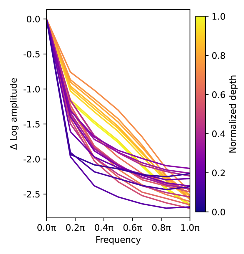
(a) ViT

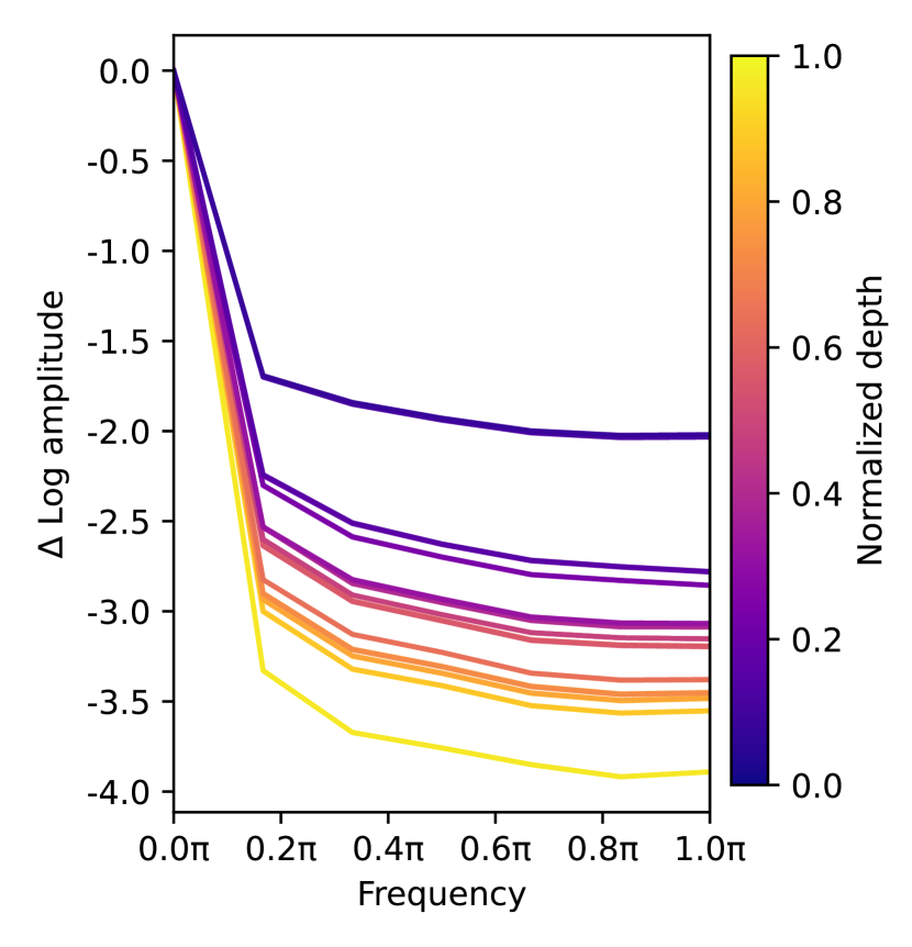
(b) GFNet

Figure 1: Relative log amplitudes of Fourier transformed feature maps. $\Delta$ Log amplitude means relative logarithmic amplitude concerning the logarithmic amplitude at normalized frequency 0. The yellower the color, the deeper the layer.

Global filters and MHSA are different in certain respects, even though they have low-pass filter characteristics like they are different in certain respects. For example, MHSA is a data-dependent operation generated from data and applied to data. In contrast, global filters multiply data and parameters and hence are less data-dependent operations. In recent works, MLP-based models, which have been less data-dependent, employ data-dependent operations (Wang et al. 2022; Rao et al. 2022), achieved accuracy improvements. It is inferred from the findings that introducing a data-dependent concept to global filters will improve accuracy.

Meanwhile, one should note that global filters have not been based on the most up-to-date and effective architectures relative to the well-researched MHSA-based and their relatives’ architectures. MetaFormer (Yu et al. 2022a, b) pays attention to the overall architecture of the Transformer. MetaFormer has a main block consisting of an arbitrary token-mixer and a channel mixer. It also makes sense to consider this framework for global filters because it is one of the most sophisticated architectures. It is necessary to close these differentials of architectural design if global filters can be a worthy alternative to MHSA modules.

We propose DFFormer, an FFT-based network to fill the above gap. Our architectures inherit MetaFormer and equip modules that can dynamically generate a global filter for each pair of feature channels in the image, considering their contents. Our experimental results show that the proposed methods achieve promising performance among vision models on the ImageNet-1K dataset, except for MHSA. DFFormer-B36 with 115M parameters has achieved a top-1 accuracy of 84.8%. CDFFormer, a hybrid architecture with convolutions and FFTs architecture, is even better. Moreover, when dealing with high-resolution images, the proposed method realizes higher throughput than the MHSA-based architecture and architecture using both CNN and MHSA. We also found that the dynamic filter tends to learn low frequency rather than MHSA on a hierarchical Metaformer.

Our main contributions are summarized as follows: First, we have introduced the dynamic filter, a dynamic version of the traditional global filter. Second, we found that injecting Metaformer-like architecture using the dynamic filter can close the gap between the accuracy of the global filter architecture and of SOTA models. Finally, through comprehensive analysis, we have demonstrated that the proposed architecture is less costly for downstream tasks of higher resolution, like dense prediction.

Related Work

Vision Transformers and Metaformers

Transformer (Vaswani et al. 2017), which was proposed in NLP, has become a dominant architecture in computer vision as well, owing to the success of ViT (Dosovitskiy et al. 2021) and DETR (Carion et al. 2020). Soon after, MLP-Mixer (Tolstikhin et al. 2021) demonstrates that MLP can also replace MHSA in Transformer. MetaFormer (Yu et al. 2022a), as an abstract class of Transformer and MLP-Mixer, was proposed as a macro-architecture. The authors tested the hypothesis using MetaFormer with pooling. Generally, the abstract module corresponding to MHSA and MLP is called a token-mixer. It emphasizes the importance of MetaFormer that new classes of MetaFormer, such as Sequencer (Tatsunami and Taki 2022) using RNNs, Vision GNN (Han et al. 2022) using graph neural networks, and RMT (Fan et al. 2023) using retention mechanism that is variant of the attention mechanism, have emerged. Moreover, a follow-up study (Yu et al. 2022b) has shown that even more highly accurate models can be developed by improving activation and hybridizing with multiple types of tokens. We retain the macro-architecture of (Yu et al. 2022b). The FFT-based module is a global operation like MHSA and can efficiently process high-resolution images without much loss of accuracy.

FFT-based Networks

In recent years, neural networks using Fourier transforms have been proposed. FNet (Lee-Thorp et al. 2022), designed for NLP, contains modules using a discrete or fast Fourier Transform to extract only the real part. Accordingly, they have no parameters. Fast-FNet (Sevim et al. 2023) removes waste and streamlines FNet. GFNet (Rao et al. 2021) is an FFT-based network designed for vision with global filters. The global filter operates in frequency space by multiplying features with a Fourier filter, equivalent to a cyclic convolution. The filter is a parameter, i.e., the same filter is used for all samples. In contrast, our dynamic filter can dynamically generate the Fourier filter using MLP. (Guibas et al. 2022) is one of the most related works and proposed AFNO. Instead of the element-wise product, the MLP operation of complex weights is used to represent an adaptive and non-separable convolution. AFNO is not a separable module. As a result, the computational cost is higher than the separable module. On the contrary, our proposed method can realize a dynamic separatable Fourier filter, and our models do not differ much from the global filter in terms of FLOPs. We will mention these throughputs in subsection Ablation Studies. Concurrent work (Vo et al. 2023) also attempts to generate dynamic filters, but the structure is such that only the filter coefficients are changed. Although the amplitude and frequency of the filter are dynamic, the major property of the filter cannot be changed (e.g., a high-pass filter cannot be changed to a low-pass filter). In contrast, a dynamic filter can represent high-pass and low-pass filters by first-order coupling.

Dynamic Weights

There have been some suggestive studies on the generation of dynamic weights. (Jia et al. 2016) realizes the filter parameters to change dynamically, where the filter weights of the convolution were model parameters. A filter generation network generates the filters. (Ha, Dai, and Le 2016) is a contemporaneous study. It proposed HyperNetworks, neural networks to create weights of another neural network. They can generate weights of CNN and RNN. (Yang et al. 2019; Chen et al. 2020) are at the same time worked on, both of which make the filters of convolution dynamic. These works influence our dynamic filter: whereas (Yang et al. 2019; Chen et al. 2020) predict the real coefficients of linear combination for a real filter basis of standard convolution, our work predicts the real coefficients of linear combination for a complex parameter filter basis. This method can be considered an equivalent operation in forward propagation from the fast Fourier transform’s linearity; thus, our work is similar to these works. In backpropagation, however, whether the proposed dynamic filter can be learned is nontrivial. Our architecture does not also need the training difficulties cited in these studies, such as restrictions on batch size or adjustment of softmax temperatures. Outside of convolution, Synthesizer (Tay et al. 2021), DynaMixer (Wang et al. 2022), and AMixer (Rao et al. 2022) have MLP-Mixer-like token-mixer, but with dynamic generation of weights. In particular, AMixer includes linear combinations related to our work.

Method

Preliminary: Global Filter

We will look back at a discrete Fourier transform before introducing a global filter (Rao et al. 2021). We discuss a 2D discrete Fourier transform (2D-DFT). For given the 2D signal $x(h,w)$, we define the 2D-DFT $\tilde{x}(h^{\prime},w^{\prime})$ as following: ~x(h’,w’) &= ∑_h=0^H-1∑_w=0^W-1 x(h,w) e-2πj(hh’H+ww’W)HW where $H,W\in\mathbb{N}$, $h,h^{\prime}\in\{z\in\mathbb{Z}\,|\,0<z<H\}$, and $w,w^{\prime}\in\{z\in\mathbb{Z}\,|\,0<z<W\}$. Its inverse transformation exists and is well-known as a 2D inverse discrete Fourier transform (2D-IDFT). Generally, $\tilde{x}(h^{\prime},w^{\prime})$ is complex and periodic to $h^{\prime}$ and $w^{\prime}$. We assume that $x(h^{\prime},w^{\prime})$ is a real number, then a complex matrix $\tilde{X}(h^{\prime},w^{\prime})$ associated with $\tilde{x}(h^{\prime},w^{\prime})$ is Hermitian. A space to which $\tilde{x}(h^{\prime},w^{\prime})$ belongs is known as a frequency domain and is available for analyzing frequencies. In addition, the frequency domain has a significant property: Multiplication in the frequency domain is equivalent to a cyclic convolution in the original domain, called convolution theorem (Proakis 2007). The 2D-DFT is impressive but has a complexity of $\mathcal{O}(H^{2}W^{2})$. Therefore, a 2D-FFT is proposed and is often used in signal processing. It is improved with complexity $\mathcal{O}(HW\log_{2}{(HW)})$.

Second, we define the global filter for the feature $\mathbf{X}\in\mathbb{R}^{C\times H\times W}$. The global filter $\mathcal{G}$ formulate the following: G(X) &= F^-1(K ⊙F(X)) where $\odot$ is the element-wise product, $\mathbf{K}\in\mathbb{C}^{C\times H\times\lceil\frac{W}{2}\rceil}$ is a learnable filter, and $\mathcal{F}$ is the 2D-FFT of which redundant components are reduced (i.e., rfft2) since $\mathcal{F}(x)$ is Hermitian. Note that the operation is equivalent to cyclic convolution of the filter $\mathcal{F}^{-1}(\mathbf{X})$ based on the convolution theorem.

The global filter is known to have some properties. (1) The theoretical complexity is $\mathcal{O}(HWC\lceil\log_{2}{(HW)}\rceil+HWC)$. It is more favorable than Transformer and MLP when input is high resolution. (2) The global filter can easily scale up the input resolution owing to interpolating the filter. See (Rao et al. 2021) for more details.

Dynamic Filter

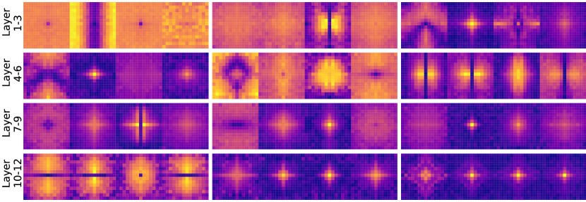
Figure 2: Filters in the frequency domain on GFNet-Ti

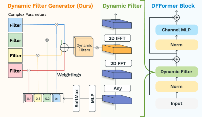
Figure 3: Dynamic Filter is our proposed component where ”Any” modules are allowed continuous real maps. DFFormer Block is a MetaFormer block equipped with the dynamic filter.

This subsection discusses a dynamic filter in which a neural network dynamically determines an adequate global filter. The left side of Figure 3 shows the dynamic filter, which has a global filter basis of which the dimension is $N$, and linearly coupled global filters for them are used for each channel instead of learnable global filters. The coefficients are ruled by an MLP $\mathcal{M}$. We specify the whole dynamic filter $\mathcal{D}$ as follows: D(X) &= F^-1(K_M(X) ⊙F∘A(X)) where $\mathcal{K}_{\mathcal{M}}$ denotes the function that determines the dynamic filter. $\mathcal{A}$ are continuous real maps, including point-wise convolutions and identity maps.

Generating Dynamic Filter

We denote global filter basis $\mathbb{K}$ so that $\mathbb{K}=\{\mathcal{K}_{1},\ldots,\mathcal{K}_{N}\}$ and $\mathcal{K}_{1},\ldots,\mathcal{K}_{N}\in\mathbb{C}^{H\times\lceil\frac{W}{2}\rceil}$. Filters $\mathcal{K}_{\mathcal{M}}(\mathbf{X})\in\mathbb{C}^{C^{\prime}\times H\times\lceil\frac{W}{2}\rceil}$ are associated with $\mathcal{M}$ for weighting and are defined by the following: K_M(X)_c,:,::=∑_i=1^N (e^s_(c-1)N+i∑_n=1^Ne^s_(c-1)N+n)K_i,
where  (s_1, …, s_NC’)^⊤= M(∑_h,wX_:,h,wHW). In this paper, we use $N=4$, which is the dimension of $\mathbb{K}$, to avoid over-computing. See ablation in subsection Ablation Studies.

MLP for weighting

We describe MLP $\mathcal{M}$ for weighting throughout specific calculation formulas:

$$\mathcal{M}(\mathbf{X})=W_{2}\texttt{StarReLU}(W_{1}\texttt{LN}(\mathbf{X})),$$ (1)

where $\texttt{LN}(\cdot)$ is layer normalization (Ba, Kiros, and Hinton 2016), $\texttt{StarReLU}(\cdot)$ is an activation function proposed by (Yu et al. 2022b), $W_{1}\in\mathbb{R}^{C\times{\tt int}(\rho C)}$, $W_{2}\in\mathbb{R}^{{\tt int}(\rho C)\times NC^{\prime}}$ denote matrices of MLP layer, $\rho$ is a ratio of the intermediate dimension to the input dimension of MLP. We choose $\rho=0.25$ but see section Ablation Studies for the other case.

DFFormer and CDFFormer

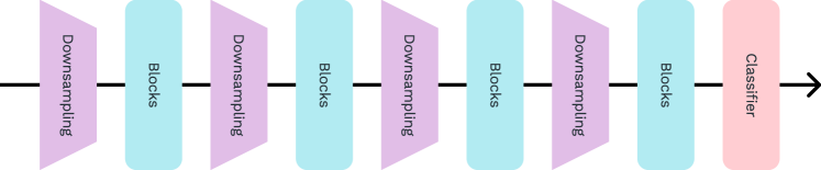
Figure 4: A four-stage model

Model		DFFormer	CDFFormer
TokenMixer		$\texttt{DF},\texttt{DF},\texttt{DF},\texttt{DF}$	$\texttt{CF},\texttt{CF},\texttt{DF},\texttt{DF}$
Down Smp.		$K=7\text{-}3\text{-}3\text{-}3$, $S=4\text{-}2\text{-}2\text{-}2$, $P=2\text{-}1\text{-}1\text{-}1$
Size	S18	$L=3\text{-}3\text{-}9\text{-}3$, $C=64\text{-}128\text{-}320\text{-}512$
	S36	$L=3\text{-}3\text{-}9\text{-}3$, $C=64\text{-}128\text{-}320\text{-}512$
	M36	$L=3\text{-}3\text{-}9\text{-}3$, $C=96\text{-}192\text{-}384\text{-}576$
	B36	$L=3\text{-}3\text{-}9\text{-}3$, $C=128\text{-}256\text{-}512\text{-}768$
Classifier		GAP, Layer Norm., MLP

Table 1: Model settings of DFFormer and CDFFormer. DF and CF mean DFFormer block and CFFormer block, respectively. $K$, $S$, $P$, $C$, and $L$ denote kernel size, stride, padding, number of channels, and number of blocks, respectively. The indices of each tuple correspond to the order of the stages.

We construct DFFormer and CDFFormer complying with MetaFormer (Yu et al. 2022b). DFFormer and CDFFormer mainly consist of MetaFormer blocks, such as DFFormer and ConvFormer blocks. DFFormer and CDFFormer blocks comply with MetaFormer blocks

$$\mathcal{T}(\mathbf{X})=\mathbf{X}+\texttt{Conv}_{\textrm{pw2}}\circ\mathcal{L}\circ\texttt{StarReLU}\circ\texttt{Conv}_{\textrm{pw1}}\circ\texttt{LN}(\mathbf{X})$$ (2)

where $\texttt{LN}(\cdot)$ is Layer Normalization (Ba, Kiros, and Hinton 2016), $\texttt{Conv}_{\textrm{pw1}}(\cdot)$ and $\texttt{Conv}_{\textrm{pw2}}(\cdot)$ are point-wise convolutions so that the number of output channels is $(C^{\prime}=)2C$ and $C$, respectively, and $\mathcal{L}(\cdot)$ is dimensional invariant any function. If $\mathcal{L}(\cdot)$ is separable convolution, $\mathcal{T}$ is named as ConvFormer block at (Yu et al. 2022b). If $\mathcal{L}(\cdot)=\mathcal{F}^{-1}(\mathcal{K}_{\mathcal{M}}(\mathbf{X})\odot\mathcal{F}(\cdot))$, we define that $\mathcal{T}$ is DFFormer block. A schematic diagram is shown on the right side of Figure 3 in order to understand the DFFormer blocks’ structure. See codes for details in the appendix.

The overall framework is also following MetaFormer (Yu et al. 2022a, b). In other words, we utilize the four-stage model in Figure 4. We prepared four sizes of models for DFFormer, which mainly consists of DFFormer blocks, and CDFFormer, which is a hybrid model of DFFormer blocks and ConvFormer blocks. Each model is equipped with an MLP classifier with Squared ReLU (So et al. 2021) as the activation. A detailed model structure is shown in Table 1.

Experiments

We conduct experiments on ImageNet-1K benchmark (Krizhevsky, Sutskever, and Hinton 2012) and perform further experiments to confirm downstream tasks such as ADE20K (Zhou et al. 2017). Finally, we will conduct ablation studies about design elements.

Image Classification

Model	Ty.	Prm. (M)	FLOP (G)	Thrp. (img/s)	Top-1 (%)
ConvNeXt-T	C	29	4.5	1471	82.1
ConvFormer-S18	C	27	3.9	756	83.0
CSWin-T	A	23	4.3	340	82.7
MViTv2-T	A	24	4.7	624	82.3
DiNAT-T	A	28	4.3	816	82.7
DaViT-Tiny	A	28	4.5	1121	82.8
GCViT-T	A	28	4.7	566	83.5
MaxViT-T	A	41	5.6	527	83.6
RMT-S	R	27	4.5	406	84.1
AMixer-T	M	26	4.5	724	82.0
GFNet-H-S	F	32	4.6	952	81.5
DFFormer-S18	F	30	3.8	535	83.2
CAFormer-S18	CA	26	4.1	741	83.6
CDFFormer-S18	CF	30	3.9	567	83.1
ConvNeXt-S	C	50	8.7	864	83.1
ConvFormer-S36	C	40	7.6	398	84.1
MViTv2-S	A	35	7.0	416	83.6
DiNAT-S	A	51	7.8	688	83.8
DaViT-Small	A	50	8.8	664	84.2
GCViT-S	A	51	8.5	478	84.3
RMT-B	R	54	9.7	264	85.0
DynaMixer-S	M	26	7.3	448	82.7
AMixer-S	M	46	9.0	378	83.5
GFNet-H-B	F	54	8.6	612	82.9
DFFormer-S36	F	46	7.4	270	84.3
CAFormer-S36	CA	39	8.0	382	84.5
CDFFormer-S36	CF	45	7.5	319	84.2
ConvNeXt-B	C	89	15.4	687	83.8
ConvFormer-M36	C	57	12.8	307	84.5
MViTv2-B	A	52	10.2	285	84.4
GCViT-S2	A	68	10.7	415	84.8
MaxViT-S	A	69	11.7	449	84.5
DynaMixer-M	M	57	17.0	317	83.7
AMixer-B	M	83	16.0	325	84.0
DFFormer-M36	F	65	12.5	210	84.6
CAFormer-M36	CA	56	13.2	297	85.2
CDFFormer-M36	CF	64	12.7	254	84.8
ConvNeXt-L	C	198	34.4	431	84.3
ConvFormer-B36	C	100	22.6	235	84.8
MViTv2-L	A	218	42.1	128	85.3
DiNAT-B	A	90	13.7	499	84.4
DaViT-Base	A	88	15.5	528	84.6
GCViT-B	A	90	14.8	367	85.0
MaxViT-B	A	120	23.4	224	85.0
RMT-L	R	95	18.2	233	85.5
DynaMixer-L	M	97	27.4	216	84.3
DFFormer-B36	F	115	22.1	161	84.8
CAFormer-B36	CA	99	23.2	227	85.5
CDFFormer-B36	CF	113	22.5	195	85.0

Table 2: Performance comparison of models pre-trained on ImageNet-1K at the resolution of $224^{2}$. Throughput has been benchmarked on a V100 with 16GB memory at a batch size of 16. The full names of types are C is Convolution, A is Attention, R is Retention, M is MLP, F is FFT, CA is a hybrid of Convolution and Attention, and a hybrid of Convolution and FFT, respectively.

DFFormers and CDFFormers have experimented on ImageNet-1K (Krizhevsky, Sutskever, and Hinton 2012), one of the most renowned data sets in computer vision for image classification. It has 1000 classes and contains 1,281,167 training images and 50,000 validation images. Our training strategy is mainly according to (Touvron et al. 2021a) and is detailed as follows. For data augmentation methods, we apply MixUp (Zhang et al. 2018), CutMix (Yun et al. 2019), random erasing (Zhong et al. 2020), and RandAugment (Cubuk et al. 2020). Stochastic depth (Huang et al. 2016) and label smoothing (Szegedy et al. 2016) are used to regularize. We employ AdamW (Loshchilov and Hutter 2019) optimizer for 300 epochs with a batch size of 1024. The base learning rate of $\frac{\rm{batch\,size}}{512}\times 5\times 10^{-4}$, 20 epochs of linear warm-up, cosine decay for learning rate, and weight decay of 0.05 are used. The implementation is based on PyTorch (Paszke et al. 2019) and timm (Wightman 2019). The details of the hyperparameters are presented in the appendix. We compare the proposed models with various family models, including CNN-based like ConvNeXt (Liu et al. 2022) and ConvFormer (Yu et al. 2022b), attention-based like DeiT (Touvron et al. 2021a), CSwin (Dong et al. 2022), MViTv2 (Li et al. 2022), DiNAT (Hassani and Shi 2022), DaViT (Ding et al. 2022a), GCViT (Hatamizadeh et al. 2023), and MaxViT (Tu et al. 2022), Retention-based like RMT (Fan et al. 2023), MLP-based like DynaMixer (Wang et al. 2022) and AMixer (Rao et al. 2022), FFT-based like GFNet (Rao et al. 2021), and hybrid models like CAFormer (Yu et al. 2022b). Table 2 shows the results. We can see that DFFormers and CDFFormers perform top-1 accuracy among models except for models using attention or retention, with comparable parameters. DFFormers are particularly state-of-the-art among traditional FFT-based models. They perform more than 0.5% better than other FFT-based models and have been ahead of MLP-based models to which FFT-based tend to compare. CDFFormers also have better cost performance than DFFormers due to using conjunction with convolution. The largest model, CDFFormer-B36, outperforms DFFormer-B36. The above performance comparison of DFFormer and CDFFormer indicates that dynamic filters are promising modules for image recognition.

Semantic Segmentation on ADE20K

Backbone	Prm. (M)	mIoU (%)
ResNet-50 (He et al. 2016)	28.5	36.7
PVT-Small (Wang et al. 2021)	28.2	39.8
PoolFormer-S24 (Yu et al. 2022a)	23.2	40.3
DFFormer-S18 (ours)	31.7	45.1
CDFFormer-S18 (ours)	31.4	44.9
ResNet-101 (He et al. 2016)	47.5	38.8
ResNeXt-101-32x4d (Xie et al. 2017)	47.1	39.7
PVT-Medium (Wang et al. 2021)	48.0	41.6
PoolFormer-S36 (Yu et al. 2022a)	34.6	42.0
DFFormer-S36 (ours)	47.2	47.5
CDFFormer-S36 (ours)	46.5	46.7
PVT-Large (Wang et al. 2021)	65.1	42.1
PoolFormer-M36 (Yu et al. 2022a)	59.8	42.4
DFFormer-M36 (ours)	66.4	47.6
CDFFormer-M36 (ours)	65.2	48.6

Table 3: Performance comparison of models using Semantic FPN trained on ADE20K. The settings follow (Yu et al. 2022a) and the results of compared models are cited from (Yu et al. 2022a).

We train and test our models on ADE20K (Zhou et al. 2017) dataset for a semantic segmentation task to evaluate the performance in dense prediction tasks. We employ Semantic FPN (Kirillov et al. 2019) in mmseg (Contributors 2020) as a base framework. See the appendix for setup details. Table 3 shows that DFFormer-based and CDFFormer-based models equipped with Semantic FPN for semantic segmentation are effective for the semantic segmentation task. They are superior to those based on other models, including PoolFormer-based models. From these results, it can be seen that DFFormer-S36 has 5.5 points higher mIoU than PoolFormer-S36. In addition, CDFFormer-M36 achieves 48.6 mIoU. As a result, we also verify the effectiveness of DFFormer and CDFFormer for semantic segmentation.

Ablation Studies

Ablation	Variant	Parameters (M)	FLOPs (G)	Throughput (img/sec)	Top-1 Acc. (%)
Baseline	DFFormer-S18	30	3.8	535	83.2
Filter	$N=4\,\rightarrow\,2$	29	3.8	534	83.0
	$\rho=0.25\,\rightarrow\,0.125$	28	3.8	532	83.1
	GFFormer-S18	30	3.8	575	82.9
	DF $\rightarrow$ AFNO	30	3.8	389	82.6
Activation	StarReLU $\rightarrow$ GELU	30	3.8	672	82.7
	StarReLU $\rightarrow$ ReLU	30	3.8	640	82.5
	StarReLU, DF$\rightarrow$ ReLU, AFNO	30	3.8	444	82.0

Table 4: Ablation for DFFormer-S18 on ImageNet-1K. Remind $N$ is the dimension of the dynamic filter basis, and $\rho$ is a ratio of MLP intermediate dimension to input dimension.

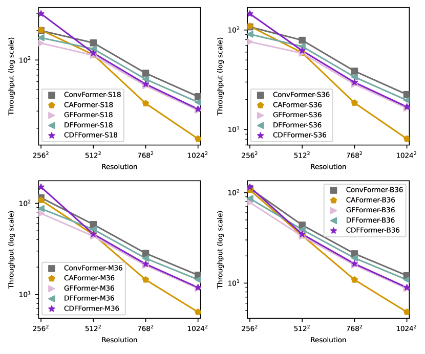
Figure 5: Throughput vs. resolution. Throughput has been benchmarked on a V100 with 16GB memory at a batch size of four.

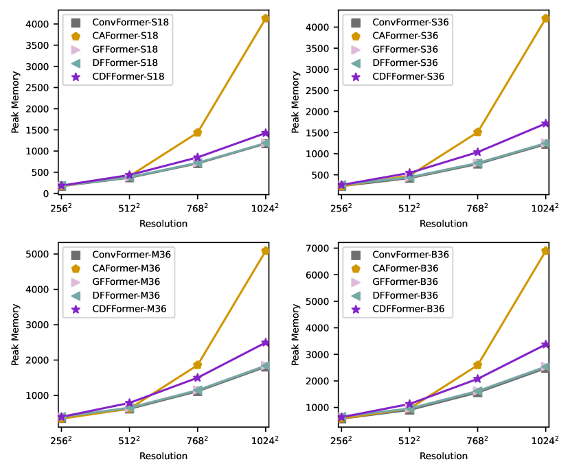
Figure 6: Peak memory vs. resolution. Peak memory has been benchmarked on a V100 with 16GB memory at a batch size of four.

We experiment with ablation studies on the ImageNet-1K dataset. Let us discuss ablation from several perspectives.

Filter

We studied how changing filters would work. First, we change to the hyperparameters of dynamic filters. Specifically, we train and test models in which the dimension of dynamic filter base $N$ and the intermediate dimension $\rho C$ are modified in half of the cases, respectively. From Table 4, however, we found that the throughput and number of parameters remained almost the same, and the accuracy dropped by 0.2% and 0.1%, respectively. Next, we train GFFormer-S18, which is replaced by each dynamic filter of DFformer-S18 with a global filter (i.e., static filter) to confirm the effectiveness of dynamic filters. Table 4 demonstrates DFformer-S18 is superior to GFFormer-S18 0.3%. We also have studied a case where AFNOs replaced dynamic filters but found that the AFNO-based model degraded in accuracy more than the dynamic filter and that dynamic filters have better throughput than AFNOs.

Activation

DFFormer and CDFFormer use StarReLU, but this is a relatively new activation; many MetaFormers employ Gaussian Error Linear Unit (GELU) (Hendrycks and Gimpel 2023), and earlier generations of convolutional neural networks (CNNs), such as ResNet (He et al. 2016), often used Rectified Linear Unit (ReLU) (Nair and Hinton 2010). Accordingly, we also experiment with a version of the model in which GELU and ReLU replace StarReLU in DFFormer-S18. As a result, Table 4 shows that DFFormer-S18 outperforms the replaced version of the model by more than 0.5%, demonstrating that StarReLU is also a valuable activation for dynamic filters. In this manner, StarReLU has a significant impact on the final performance. Therefore, to comprehend how much a dynamic filter would improve performance without StarReLU, we also experimented with a model version in which StartReLU and a dynamic filter are replaced by ReLU and AFNO, respectively. Comparing this result with the StarReLU $\to$ ReLU results shows us that the dynamic filter has enough impact even when the influence of StarReLU is removed.

Analysis

Advantages at Higher Resolutions

We observe how the throughput and peak memory at inference change on proposed and comparative models when resolution varies. For throughput, the proposed models have been inferior to CAFormer, an architecture that utilized MHSA, at a resolution of $224^{2}$ since Table 2 can comprehend the fact. The result conflicts with the computational complexity presented in the Introduction. Our interpretation of the issue is that the actual throughput would depend on the implementation of FFT (although we use cuFFT via PyTorch), hardware design, etc. Increasing the resolution, the theoretically computational complexity of MHSA comes into effect: Figure 5 shows the throughput for different resolutions. DFFormer and CDFFormer maintain throughput close to that of ConvFormer, while only CAFormer shows a significant decrease in throughput. The same is true for peak memory in Figure 6: Whereas the CAFormer peak memory increases, the DFFormer and CDFFormer peak memory is comparable to that of ConvFormer. Therefore, DFFormer and CDFFormer are beneficial in speed- and memory-constrained environments for tasks such as semantic segmentation, where high resolution is required.

Representational Similarities

Figure 7 shows the similarities between GFFormer-S18 and DFFormer-S18, ConvFormer-S18 and DFFormer-S18, and CAFormer-S18 and CDFFormer-S18 in the validation set of ImageNet-1K. In our analysis, we metric the similarity using mini-batch linear CKA (Nguyen, Raghu, and Kornblith 2021). torch_cka (Subramanian 2021) toolbox was used to implement the mini-batch linear CKA. The layers to be analyzed included four downsampled and 18 token-mixers residual blocks and 18 channel MLP residual blocks, and the indices in the figure are ordered from the shallowest layer. Figure 7 shows that GFFormer-S18 and DFFormer-S18 are very similar up to stage 3, although they are slightly different at stage 4. We also found the same thing about the similarity between ConvFormer-S18 and DFFormer-S18 from Figure 7. On the contrary, Figure 7 shows that CAFormer-S18 and CDFFormer-S18 are similar up to stage 2 with convolution but become almost entirely different from stage 3 onward. Even though FFT-based token-mixers, like MHSA, are token-mixers in the global domain and can capture low-frequency features, they necessarily do not learn similar representations. The fact would hint that MHSA and the FFT-based token-mixer have differences other than spatial mixing.

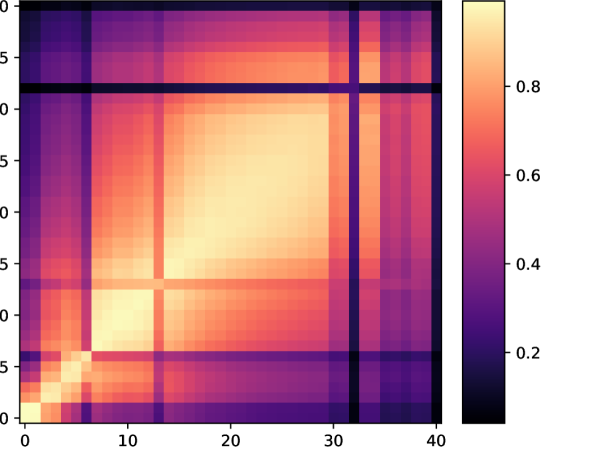
(a) GF vs. DF

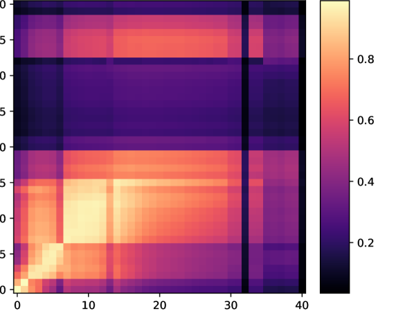
(b) CA vs. CDF

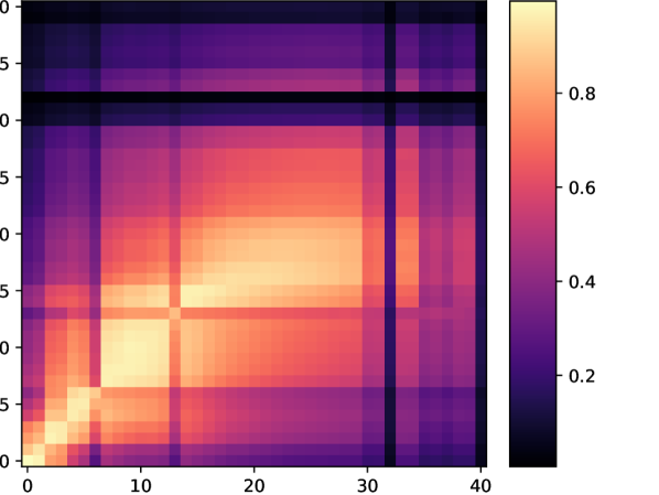
(c) Conv vs. DF

Figure 7: The feature map similarities by CKA

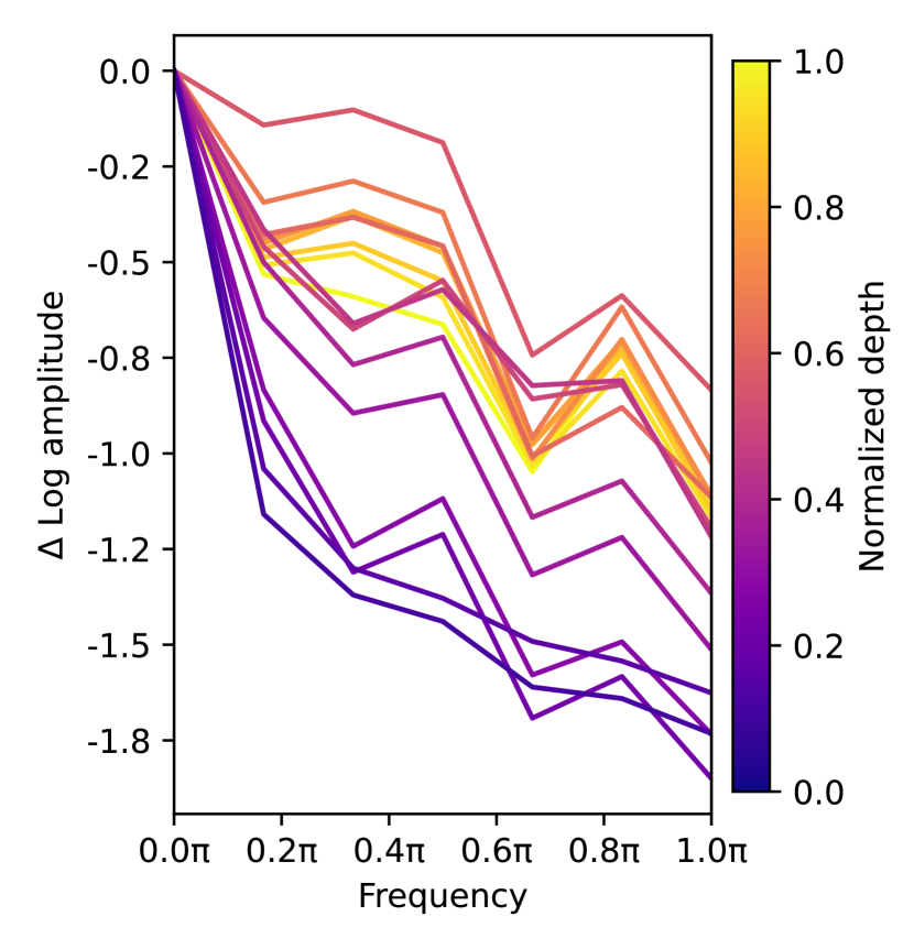
(a) CAFormer-S18

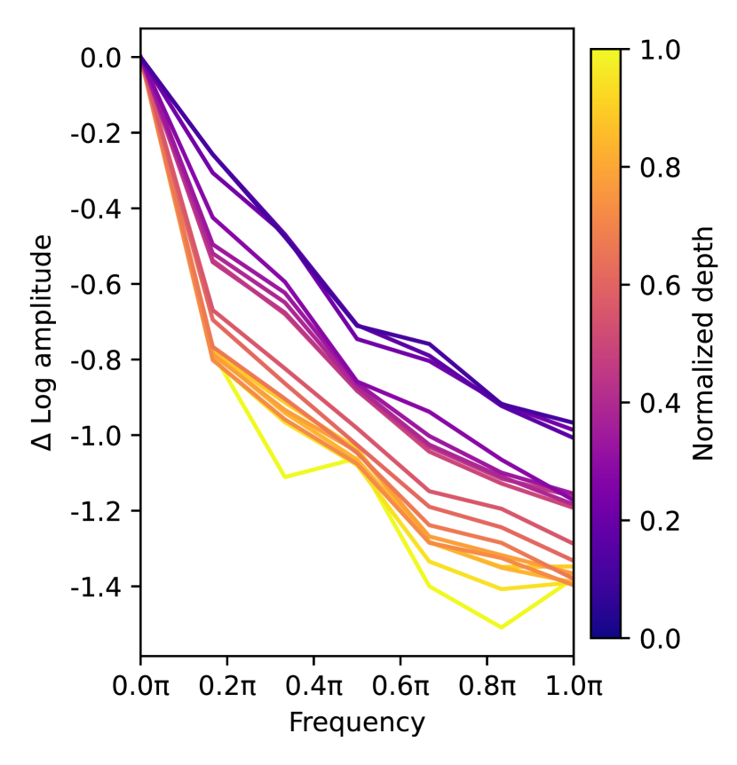
(b) CDFFormer-S18

Figure 8: Relative log amplitudes of Fourier transformed feature maps on stage 3. A setup similar to that in Table 1.

We perform a Fourier analysis on stage 3 to know the difference in stage 3. Figure 8 shows the difference between MHSA and FFT-based token-mixer results. Surprisingly, CAFormer-S18 acts as a high-pass filter, whereas the result for CDFFormer-S18 indicates more attenuated at other frequencies than around 0. In other words, MHSA incorporated in a hierarchical architecture can learn high-pass and low-pass filters while the dynamic filter attenuates the high frequencies. Only applying to stage 3 makes the analysis more interpretable than overall because this analysis drastically changes frequency by downsampling.

Analysis of Dynamic Filter Basis

The basis of complex parameters in the frequency domain can represent dynamic filters used in DFFormer and CDFFormer. Here, we visualize them for DFFormer-S18, which has four in each dynamic filter module. In our visualization, the center pixel means zero frequency and the yellower pixel means higher amplitudes. Figure 9 demonstrates that the redundancy of filters in the same layer is reduced compared to Figure 2 about GFNet-Ti. In addition, we can see high-pass, low-pass, and band-pass filters in many layers. Details of the visualization method and more visualization will be given in the appendix.

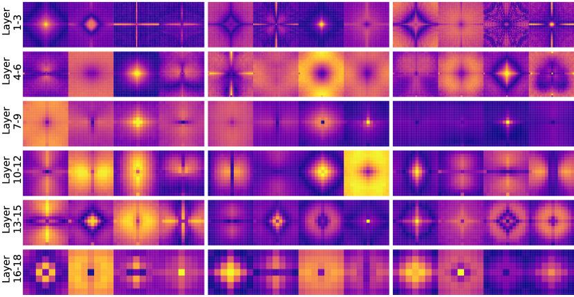
Figure 9: Filters in the frequency domain on DFFormer-S18

Conclusion

This paper studied the similarities and differences between the global filter and MHSA in vision models. According to the analysis, we proposed a novel dynamic filter responsible for dynamically generating global filters. Based on this module, we have developed new MetaFormer classes, DFFormer and CDFFormer, which achieve promising performance in MHSA-free MetaFormers. We have proven through a variety of experiments that the proposed models perform impressively not only in image classification but also in downstream tasks. In addition, our models can process high-resolution images faster and with less memory than MetaFormers using MHSA. We also found that the representation and properties of our models are not similar unexpectedly to that of models using MHSA.

Appendix A More Experiment

Object Detection on COCO

l—ccccccc Backbone Parameters(M) AP(%) AP₅₀ AP₇₅(%) AP_S(%) AP_M(%) AP_L(%)
ResNet-50 37.7 36.3 55.3 38.6 19.3 40.0 48.8
PoolFormer-S24 31.1 38.9 59.7 41.3 23.3 42.1 51.8
DFFormer-S18 (ours) 38.1 43.6 64.5 46.6 27.5 47.3 58.1
CDFFormer-S18 (ours) 37.4 43.4 64.7 46.3 26.3 47.1 57.3
ResNet-101 56.7 38.5 57.8 41.2 21.4 42.6 51.1
PoolFormer-S36 40.6 39.5 60.5 41.8 22.5 42.9 52.4
DFFormer-S36 (ours) 53.8 45.3 66.1 48.7 26.9 49.0 59.9
CDFFormer-S36 (ours) 52.6 45.0 66.0 47.8 27.6 48.5 59.6
We evaluate the performance of our models on downstream tasks, especially in object detection on COCO benchmark (Lin et al. 2014). It has 80 classes consisting of 118,287 training images and 5,000 validation images. We employ RetinaNet as an object detection framework. The implementation takes (Lin et al. 2017) of mmdet (Chen et al. 2019). We utilize pre-trained models on ImageNet-1K dataset as the backbones. Following the setting in (Yu et al. 2022a), we use 1$\times$ training, meaning 12 epochs, batch size of 16, and AdamW (Loshchilov and Hutter 2019) optimizer with an initial learning rate of $10^{-4}$. Similar to the general setup, training images of coco are resized to no more than 800 pixels on the short side and 1,333 pixels on the long side, keeping the aspect ratio. The testing images are also resized to 800 pixels on the short side. The default dynamic filter does not support arbitrary resolutions because of using the element-wise product. Although input images have an indeterminate resolution in the setting, pre-trained DFFormer and CDFFormer are bound with the resolution of $224^{2}$. To cancel this problem, we bicubic interpolate global filter basis $\mathbb{K}$ to fit images with a resolution of $800^{2}$ and let them be new parameters. Moreover, the global filter basis is interpolated to adjust to the shape of frequency features input to dynamic filters.

Table 5: Performance comparison of models using RetinaNet trained on COCO. The settings follow (Yu et al. 2022a) and the results of compared models are cited from (Yu et al. 2022a).

Table A shows RetinaNets with DFFormer and CDFFormer as backbones outperform comparable ResNet and PoolFormer backbones. For instance, DFFormer-S36 has 5.8 points higher AP than PoolFormer-S36. Thus, DFFormer and CDFFormer obtained competitive results in COCO object detection.

Settings of Semantic Segmentation on ADE20K

We remark on the datasets and settings of the semantic segmentation task experiments described in the main text. We use ADE20K (Zhou et al. 2017) dataset, which has 150 semantic categories, 20,210 images for training, 2,000 for validation, and 3,000 for testing. We employ Semantic FPN (Kirillov et al. 2019) in mmseg (Contributors 2020) as a base framework. Training images are resized and cropped to a shape of $512^{2}$. For testing, images are resized to a shorter size of 512 pixels, keeping the aspect ratio. We adopt global filter basis parameters $\mathbb{K}$ interpolated from pre-trained parameters to suit images with a resolution of $512^{2}$. For testing, $\mathbb{K}$ is also interpolated for the same reason as subsection A. We utilize AdamW (Loshchilov and Hutter 2019) optimizer, initial learning rate of $2\times 10^{-4}$, polynomial scheduler with a power 0.9, batch size of 32, and 40K iterations, following (Yu et al. 2022a).

Appendix B More Analysis

More Visualization of Dynamic Filter Basis

Visualization of the dynamic filter basis in models which we do not mention in the main text, is shown in Figure 10, 11.

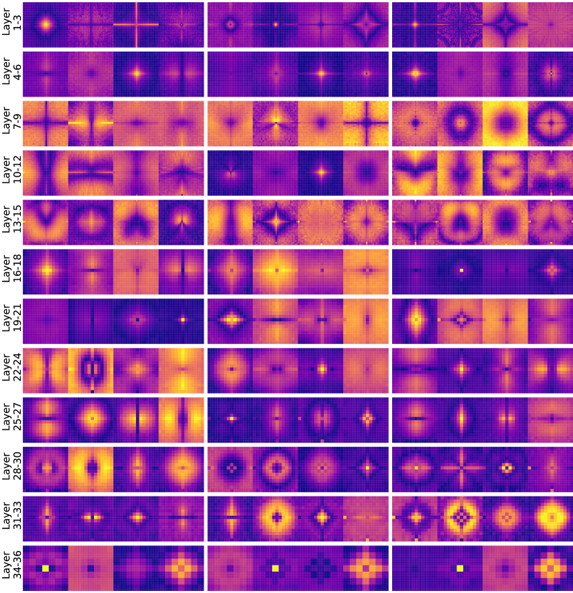
(a) DFFormer-S36

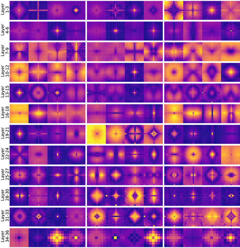
(b) DFFormer-M36

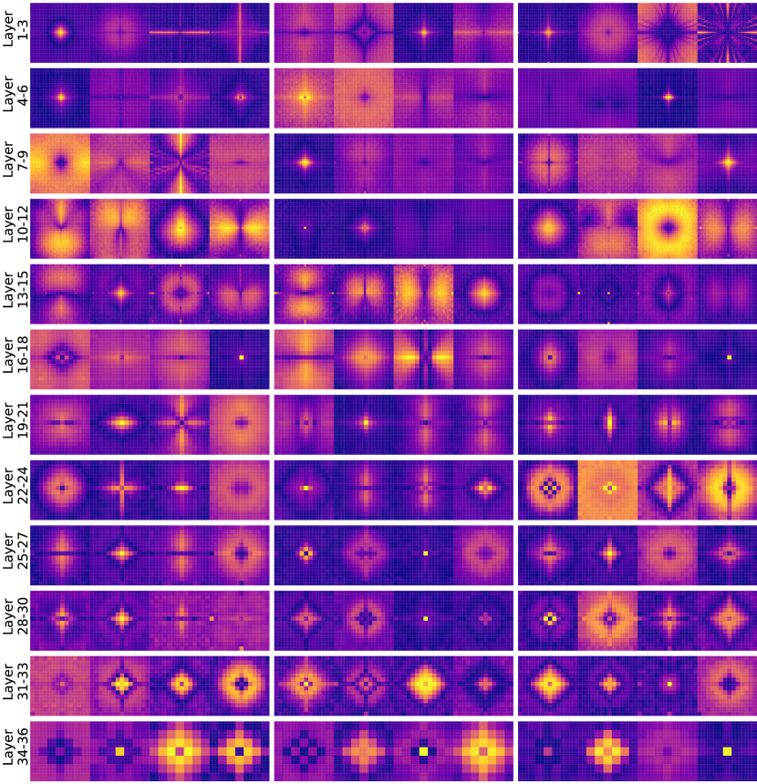
(c) DFFormer-B36

Figure 10: Visualization of dynamic filter basis in the frequency domain on DFFormers

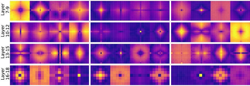
(a) CDFFormer-S18

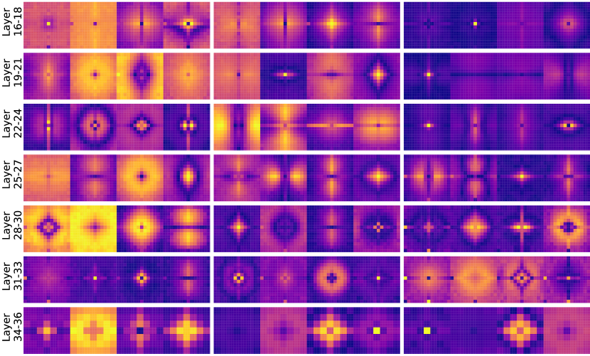
(b) CDFFormer-S36

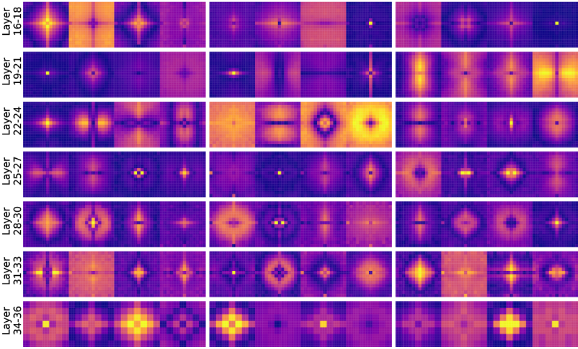
(c) CDFFormer-M36

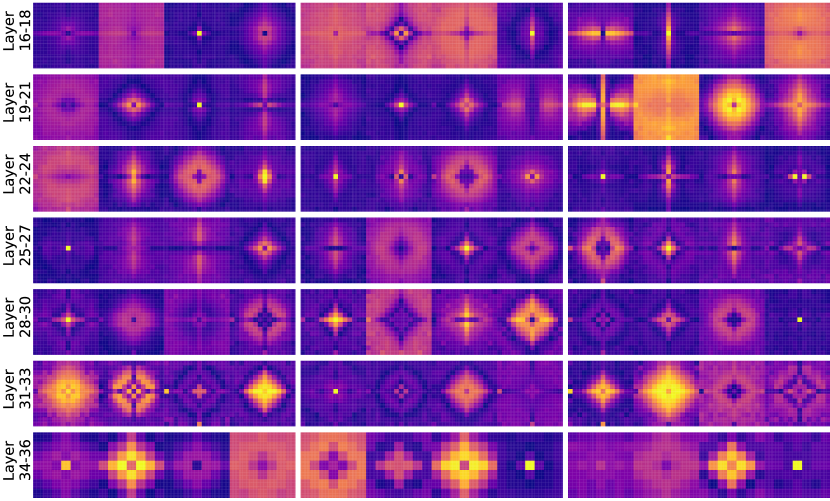
(d) CDFFormer-B36

Figure 11: Visualization of dynamic filter basis in the frequency domain on CDFFormers

More Models vs Human on Shape Bias

A brief review of previous studies on shape bias shows that FFT-based token-mixers are expected to have more intense shape bias than not global token-mixers. In earlier studies, (Baker et al. 2018), CNNs are known to be insensitive to global shape information and instead demonstrate a strong reaction to a texture. Later, (Hermann, Chen, and Kornblith 2020) point out that several data augmentations reduce texture bias and (Tuli et al. 2021) that Transformers have more substantial shape bias than CNN. (Ding et al. 2022b) found that even CNNs can improve the shape bias due to a larger kernel size. Since the FFT-based model performs operations equivalent to those of a large kernel CNN, we expected that the FFT-based model would have a similar trend to CNNs with large kernels about shape bias, and we obtained such results on S18 scale models.

We already have discussed shape bias on S18 scale models, but similarly for other scales. Figure 12 shows them of other scale models. The results tend to be the same as on S18 scale models.

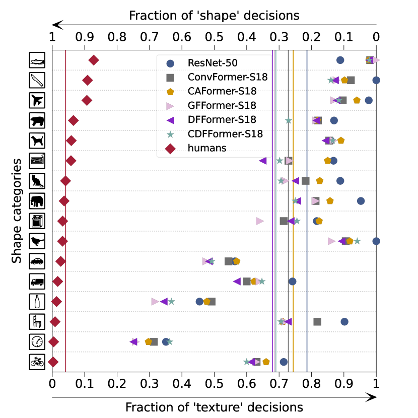
(a) S18 models vs human on shape bias

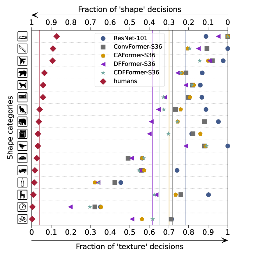
(b) S36 models vs human on shape bias

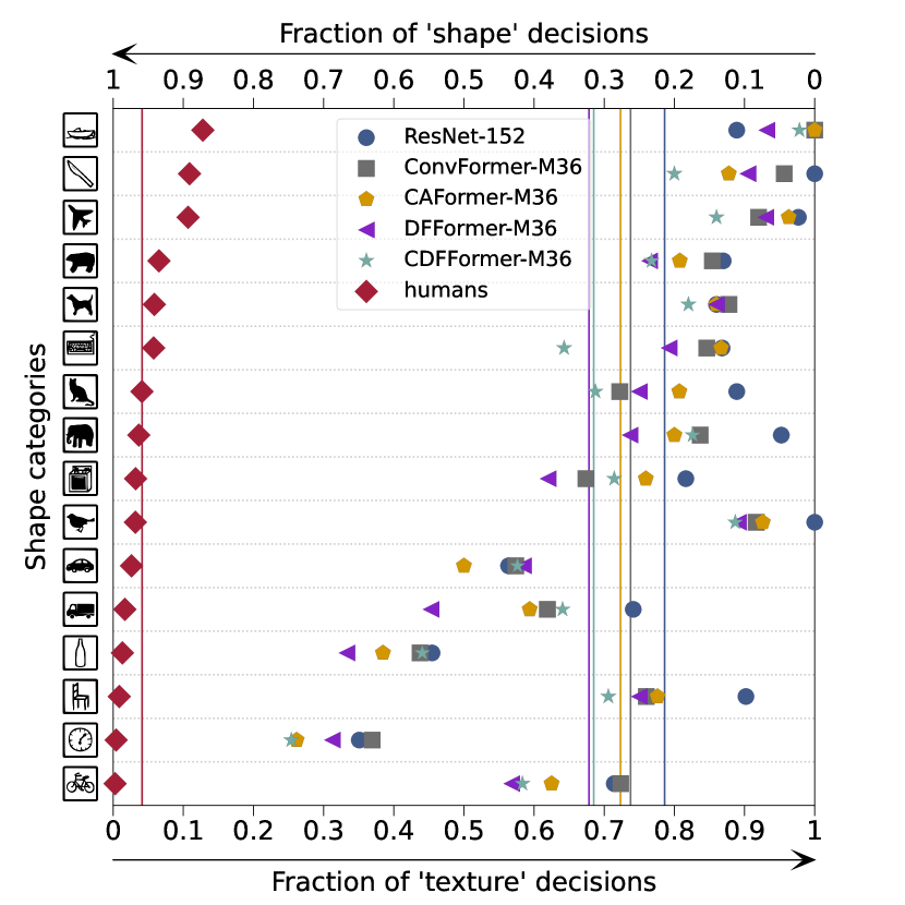
(c) M36 models vs human on shape bias

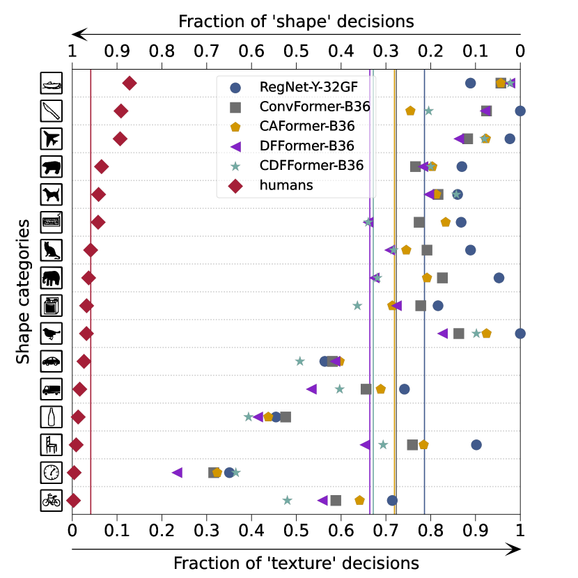
(d) B36 models vs human on shape bias

Figure 12: More shape bias

Appendix C Detailed information

Code for Dynamic Filter

The proposed dynamic filter can be implemented briefly by PyTorch (Paszke et al. 2019). Algorithm 1 shows the pseudocode for crucial parts of the dynamic filter.

Algorithm 1 Pseudocode for dynamic filter (PyTorch-like)

⬇

1class DynamicFilter(nn.Module):

2 def __init__(self, dim, expansion_ratio=2, bias=False, num_filters=4, size=14, **kwargs):

3 super().__init__()

4 size = to_2tuple(size)

5 self.size = size[0]

6 self.filter_size = size[1] // 2 + 1

7 self.num_filters = num_filters

8 self.dim = dim

9 self.med_channels = int(expansion_ratio * dim)

10 self.pwconv1 = nn.Linear(dim, self.med_channels, bias=bias)

11 self.act = StarReLU()

12 self.reweight = Mlp(dim, .25, num_filters * self.med_channels)

13 self.complex_weights = nn.Parameter(

14 torch.randn(self.size, self.filter_size, num_filters, 2,

15 dtype=torch.float32) * 0.02)

16 self.pwconv2 = nn.Linear(self.med_channels, dim, bias=bias)

17

18 def forward(self, x):

19 B, H, W, _ = x.shape

20

21 routeing = self.reweight(x.mean(dim=(1, 2))).view(B, self.num_filters, -1).softmax(dim=1)

22 x = self.pwconv1(x)

23 x = self.act(x)

24 x = x.to(torch.float32)

25 x = torch.fft.rfft2(x, dim=(1, 2), norm=’ortho’)

26 complex_weights = torch.view_as_complex(self.complex_weights)

27 routeing = routeing.to(torch.complex64)

28 weight = torch.einsum(’bfc,hwf->bhwc’, routeing, complex_weights)

29 weight = weight.view(-1, self.size, self.filter_size, self.med_channels)

30 x = x * weight

31 x = torch.fft.irfft2(x, s=(H, W), dim=(1, 2), norm=’ortho’)

32 x = self.pwconv2(x)

33 return x

34

35

36class Mlp(nn.Module):

37 def __init__(self, dim, mlp_ratio, out_features=None, bias=False, **kwargs):

38 super().__init__()

39 in_features = dim

40 out_features = out_features or in_features

41 hidden_features = int(mlp_ratio * in_features)

42

43 self.fc1 = nn.Linear(in_features, hidden_features, bias=bias)

44 self.act = StarReLU()

45 self.fc2 = nn.Linear(hidden_features, out_features, bias=bias)

46

47 def forward(self, x):

48 x = self.fc1(x)

49 x = self.act(x)

50 x = self.fc2(x)

51 return x

Code for Visualization

We utilized Algorithm 2 to visualize the complex parameters on the frequency domain in the global filter and dynamic filter.

Algorithm 2 Pseudocode of visualization of weights in global and dynamic filters (PyTorch-like)

⬇

1def visualize(weight):

2 # weight.shape: (height, width, number_of_filter, 2)

3 # weight.dtype: torch.float

4 weight = torch.view_as_complex(weight)

5 amplitude = weight.abs() + 1e-6

6 amplitude = amplitude.log()

7 amplitude = amplitude.sigmoid()

8 h, w, _ = amplitude.shape

9 if h % 2 == 0:

10 amplitude = torch.cat([amplitude, torch.flip(amplitude[:, 1:-1], dims=[1])], dim=1)

11 else:

12 amplitude = torch.cat([amplitude, torch.flip(amplitude[:, 1:], dims=[1])], dim=1)

13 h, w, _ = amplitude.shape

14 amplitude = torch.roll(amplitude, shifts=(int(h / 2), int(w / 2)), dims=(0, 1))

15 return amplitude

ImageNet-1K Training Setting

We provide ImageNet-1K training settings in Table C. These settings are used in the main results.

lc Training config. DFFormer- & CDFFormer- S18/S36/M36/B36
dataset ImageNet-1K (Krizhevsky, Sutskever, and Hinton 2012)
resolution $224^{2}$
optimizer AdamW (Loshchilov and Hutter 2019)
base learning rate 1e-3
weight decay 0.05
optimizer $\epsilon$ 1e-8
optimizer momentum $\beta_{1},=0.9,\beta_{2}{=}0.999$
batch size 1024
training epochs 300
learning rate schedule cosine decay
lower learning rate bound 1e-6
warmup epochs 20
warmup schedule linear
warmup learning rate 1e-6
cooldown epochs 10
crop ratio 1.0
RandAugment (Cubuk et al. 2020) (9, 0.5)
Mixup $\alpha$ (Zhang et al. 2018) 0.8
CutMix $\alpha$ (Yun et al. 2019) 1.0
random erasing (Zhong et al. 2020) 0.25
label smoothing (Szegedy et al. 2016) 0.1
stochastic depth (Huang et al. 2016) 0.2/0.3/0.4/0.6
LayerScale (Touvron et al. 2021b) init. None
ResScale (Shleifer, Weston, and Ott 2021) init. 1.0 (only for the last two stages)

Table 6: Hyper-parameters of classification on ImageNet-1K

Replacement of Filters in Ablation

We replaced dynamic filters with global filters and AFNOs in the ablation study. Here, we describe how to replace them. When replaced by global filters, $\mathcal{L}$ is defined as follows:

$$\mathcal{L}(\cdot)=\mathcal{G}(\cdot).$$ (3)

If replaced by AFNOs,

$$\mathcal{L}(\cdot)=\texttt{AFNO}(\cdot).$$ (4)

Detail of Advantages at Higher Resolutions

We discussed the throughput and peak memory changes during inference when varying the resolution. In the main text, the original measurements of the plotted results are listed in Table 7.

		Throughput(images/s)				Peak memory (MB)
Size	Model\Resolution	$256^{2}$	$512^{2}$	$768^{2}$	$1024^{2}$	$256^{2}$	$512^{2}$	$768^{2}$	$1024^{2}$
S18	ConvFormer	199.88	149.70	73.25	42.26	171	371	707	1175
	CAFormer	202.64	113.31	35.91	15.61	169	407	1435	4131
	DFFormer	148.59	111.81	54.45	30.54	183	385	723	1192
	CDFFormer	168.99	129.86	63.60	36.97	183	384	720	1188
S36	ConvFormer	107.43	78.95	38.66	22.51	232	421	757	1225
	CAFormer	109.14	59.07	18.53	8.08	229	481	1509	4205
	DFFormer	76.18	58.46	28.55	16.39	265	444	782	1254
	CDFFormer	90.67	68.48	33.73	19.70	263	441	778	1246
M36	ConvFormer	115.30	58.67	28.31	16.33	351	620	1116	1808
	CAFormer	108.48	45.38	14.53	6.43	340	625	1856	5088
	DFFormer	77.51	43.67	20.89	11.69	397	653	1151	1846
	CDFFormer	87.58	51.87	24.95	14.58	393	648	1145	1837
B36	ConvFormer	111.39	43.84	21.16	12.13	577	907	1563	2479
	CAFormer	106.96	33.60	10.89	4.79	583	960	2592	6895
	DFFormer	77.90	33.03	15.85	8.71	663	966	1624	2545
	CDFFormer	86.22	39.03	18.93	10.89	655	959	1615	2531

Table 7: Throughput vs. resolution and peak memory vs. resolution these have been benchmarked on a V100 with 16GB memory at a batch size of four. In this paper, we propose the models highlighted with pink as shown are proposed in this paper.

References

- Ba, Kiros, and Hinton (2016) Ba, J. L.; Kiros, J. R.; and Hinton, G. E. 2016. Layer Normalization. In NeurIPS.
- Baker et al. (2018) Baker, N.; Lu, H.; Erlikhman, G.; and Kellman, P. J. 2018. Deep convolutional networks do not classify based on global object shape. PLoS computational biology, 14(12): e1006613.
- Bertasius, Wang, and Torresani (2021) Bertasius, G.; Wang, H.; and Torresani, L. 2021. Is space-time attention all you need for video understanding? In ICML.
- Beyer et al. (2023) Beyer, L.; Izmailov, P.; Kolesnikov, A.; Caron, M.; Kornblith, S.; Zhai, X.; Minderer, M.; Tschannen, M.; Alabdulmohsin, I.; and Pavetic, F. 2023. FlexiViT: One Model for All Patch Sizes. arXiv:2212.08013.
- Carion et al. (2020) Carion, N.; Massa, F.; Synnaeve, G.; Usunier, N.; Kirillov, A.; and Zagoruyko, S. 2020. End-to-end object detection with transformers. In ECCV, 213–229. Springer.
- Chen, Panda, and Fan (2022) Chen, C.-F.; Panda, R.; and Fan, Q. 2022. Regionvit: Regional-to-local attention for vision transformers. In ICLR.
- Chen et al. (2019) Chen, K.; Wang, J.; Pang, J.; Cao, Y.; Xiong, Y.; Li, X.; Sun, S.; Feng, W.; Liu, Z.; Xu, J.; Zhang, Z.; Cheng, D.; Zhu, C.; Cheng, T.; Zhao, Q.; Li, B.; Lu, X.; Zhu, R.; Wu, Y.; Dai, J.; Wang, J.; Shi, J.; Ouyang, W.; Loy, C. C.; and Lin, D. 2019. MMDetection: Open MMLab Detection Toolbox and Benchmark. arXiv:1906.07155.
- Chen et al. (2020) Chen, Y.; Dai, X.; Liu, M.; Chen, D.; Yuan, L.; and Liu, Z. 2020. Dynamic convolution: Attention over convolution kernels. In CVPR, 11030–11039.
- Chu et al. (2021) Chu, X.; Tian, Z.; Wang, Y.; Zhang, B.; Ren, H.; Wei, X.; Xia, H.; and Shen, C. 2021. Twins: Revisiting the design of spatial attention in vision transformers. Advances in Neural Information Processing Systems, 34: 9355–9366.
- Contributors (2020) Contributors, M. 2020. MMSegmentation: OpenMMLab Semantic Segmentation Toolbox and Benchmark. https://github.com/open-mmlab/mmsegmentation.
- Cubuk et al. (2020) Cubuk, E. D.; Zoph, B.; Shlens, J.; and Le, Q. V. 2020. RandAugment: Practical automated data augmentation with a reduced search space. In CVPRW, 702–703.
- Ding et al. (2022a) Ding, M.; Xiao, B.; Codella, N.; Luo, P.; Wang, J.; and Yuan, L. 2022a. Davit: Dual attention vision transformers. In ECCV, 74–92. Springer.
- Ding et al. (2022b) Ding, X.; Zhang, X.; Zhou, Y.; Han, J.; Ding, G.; and Sun, J. 2022b. Scaling Up Your Kernels to 31x31: Revisiting Large Kernel Design in CNNs. In CVPR.
- Dong et al. (2022) Dong, X.; Bao, J.; Chen, D.; Zhang, W.; Yu, N.; Yuan, L.; Chen, D.; and Guo, B. 2022. Cswin transformer: A general vision transformer backbone with cross-shaped windows. In CVPR.
- Dosovitskiy et al. (2021) Dosovitskiy, A.; Beyer, L.; Kolesnikov, A.; Weissenborn, D.; Zhai, X.; Unterthiner, T.; Dehghani, M.; Minderer, M.; Heigold, G.; Gelly, S.; et al. 2021. An Image is Worth 16x16 Words: Transformers for Image Recognition at Scale. In ICLR.
- Fan et al. (2023) Fan, Q.; Huang, H.; Chen, M.; Liu, H.; and He, R. 2023. Rmt: Retentive networks meet vision transformers. arXiv:2309.11523.
- Guibas et al. (2022) Guibas, J.; Mardani, M.; Li, Z.; Tao, A.; Anandkumar, A.; and Catanzaro, B. 2022. Adaptive fourier neural operators: Efficient token mixers for transformers. In ICLR.
- Guo et al. (2021) Guo, M.-H.; Cai, J.-X.; Liu, Z.-N.; Mu, T.-J.; Martin, R. R.; and Hu, S.-M. 2021. Pct: Point cloud transformer. Computational Visual Media, 7(2): 187–199.
- Ha, Dai, and Le (2016) Ha, D.; Dai, A.; and Le, Q. V. 2016. Hypernetworks. In ICLR.
- Han et al. (2022) Han, K.; Wang, Y.; Guo, J.; Tang, Y.; and Wu, E. 2022. Vision gnn: An image is worth graph of nodes. In NeurIPS.
- Hassani and Shi (2022) Hassani, A.; and Shi, H. 2022. Dilated neighborhood attention transformer. arXiv:2209.15001.
- Hatamizadeh et al. (2023) Hatamizadeh, A.; Yin, H.; Heinrich, G.; Kautz, J.; and Molchanov, P. 2023. Global context vision transformers. In ICML, 12633–12646. PMLR.
- He et al. (2016) He, K.; Zhang, X.; Ren, S.; and Sun, J. 2016. Deep Residual Learning for Image Recognition. In CVPR, 770–778.
- Hendrycks and Gimpel (2023) Hendrycks, D.; and Gimpel, K. 2023. Gaussian Error Linear Units (GELUs). arXiv:1606.08415.
- Hermann, Chen, and Kornblith (2020) Hermann, K.; Chen, T.; and Kornblith, S. 2020. The origins and prevalence of texture bias in convolutional neural networks. In NeurIPS, volume 33, 19000–19015.
- Huang et al. (2016) Huang, G.; Sun, Y.; Liu, Z.; Sedra, D.; and Weinberger, K. Q. 2016. Deep Networks with Stochastic Depth. In ECCV, 646–661.
- Jia et al. (2016) Jia, X.; De Brabandere, B.; Tuytelaars, T.; and Gool, L. V. 2016. Dynamic filter networks. In NeurIPS, volume 29.
- Kirillov et al. (2019) Kirillov, A.; Girshick, R.; He, K.; and Dollár, P. 2019. Panoptic feature pyramid networks. In CVPR, 6399–6408.
- Krizhevsky, Sutskever, and Hinton (2012) Krizhevsky, A.; Sutskever, I.; and Hinton, G. E. 2012. ImageNet Classification with Deep Convolutional Neural Networks. In NeurIPS, volume 25, 1097–1105.
- Lee-Thorp et al. (2022) Lee-Thorp, J.; Ainslie, J.; Eckstein, I.; and Ontanon, S. 2022. Fnet: Mixing tokens with fourier transforms. In NAACL.
- Li et al. (2022) Li, Y.; Wu, C.-Y.; Fan, H.; Mangalam, K.; Xiong, B.; Malik, J.; and Feichtenhofer, C. 2022. MViTv2: Improved Multiscale Vision Transformers for Classification and Detection. In CVPR, 4804–4814.
- Lin et al. (2017) Lin, T.-Y.; Goyal, P.; Girshick, R.; He, K.; and Dollár, P. 2017. Focal Loss for Dense Object Detection. In ICCV, 2980–2988.
- Lin et al. (2014) Lin, T.-Y.; Maire, M.; Belongie, S.; Hays, J.; Perona, P.; Ramanan, D.; Dollár, P.; and Zitnick, C. L. 2014. Microsoft coco: Common objects in context. In ECCV, 740–755.
- Liu et al. (2023) Liu, S.; Chen, T.; Chen, X.; Chen, X.; Xiao, Q.; Wu, B.; Pechenizkiy, M.; Mocanu, D.; and Wang, Z. 2023. More convnets in the 2020s: Scaling up kernels beyond 51x51 using sparsity. In ICLR.
- Liu et al. (2021) Liu, Z.; Lin, Y.; Cao, Y.; Hu, H.; Wei, Y.; Zhang, Z.; Lin, S.; and Guo, B. 2021. Swin Transformer: Hierarchical Vision Transformer using Shifted Windows. In ICCV.
- Liu et al. (2022) Liu, Z.; Mao, H.; Wu, C.-Y.; Feichtenhofer, C.; Darrell, T.; and Xie, S. 2022. A ConvNet for the 2020s. In CVPR.
- Loshchilov and Hutter (2019) Loshchilov, I.; and Hutter, F. 2019. Decoupled Weight Decay Regularization. In ICLR.
- Nair and Hinton (2010) Nair, V.; and Hinton, G. E. 2010. Rectified linear units improve restricted boltzmann machines. In ICML.
- Neimark et al. (2021) Neimark, D.; Bar, O.; Zohar, M.; and Asselmann, D. 2021. Video transformer network. In ICCV, 3163–3172.
- Nguyen, Raghu, and Kornblith (2021) Nguyen, T.; Raghu, M.; and Kornblith, S. 2021. Do wide and deep networks learn the same things? uncovering how neural network representations vary with width and depth. In ICLR.
- Park and Kim (2022) Park, N.; and Kim, S. 2022. How Do Vision Transformers Work? In ICLR.
- Paszke et al. (2019) Paszke, A.; Gross, S.; Massa, F.; Lerer, A.; Bradbury, J.; Chanan, G.; Killeen, T.; Lin, Z.; Gimelshein, N.; Antiga, L.; et al. 2019. Pytorch: An imperative style, high-performance deep learning library. In NeurIPS, volume 32.
- Proakis (2007) Proakis, J. G. 2007. Digital signal processing: principles, algorithms, and applications, 4/E. Pearson Education India.
- Rao et al. (2022) Rao, Y.; Zhao, W.; Zhou, J.; and Lu, J. 2022. AMixer: Adaptive Weight Mixing for Self-attention Free Vision Transformers. In ECCV, 50–67. Springer.
- Rao et al. (2021) Rao, Y.; Zhao, W.; Zhu, Z.; Lu, J.; and Zhou, J. 2021. Global filter networks for image classification. In NeurIPS, volume 34.
- Sevim et al. (2023) Sevim, N.; Özyedek, E. O.; Şahinuç, F.; and Koç, A. 2023. Fast-FNet: Accelerating Transformer Encoder Models via Efficient Fourier Layers. arXiv:2209.12816.
- Shleifer, Weston, and Ott (2021) Shleifer, S.; Weston, J.; and Ott, M. 2021. NormFormer: Improved Transformer Pretraining with Extra Normalization. arXiv:2110.09456.
- So et al. (2021) So, D. R.; Mańke, W.; Liu, H.; Dai, Z.; Shazeer, N.; and Le, Q. V. 2021. Primer: Searching for efficient transformers for language modeling. In NeurIPS.
- Subramanian (2021) Subramanian, A. 2021. torch_cka. https://github.com/AntixK/PyTorch-Model-Compare.
- Szegedy et al. (2016) Szegedy, C.; Vanhoucke, V.; Ioffe, S.; Shlens, J.; and Wojna, Z. 2016. Rethinking the Inception Architecture for Computer Vision. In CVPR, 2818–2826.
- Tatsunami and Taki (2022) Tatsunami, Y.; and Taki, M. 2022. Sequencer: Deep LSTM for Image Classification. In NeurIPS.
- Tay et al. (2021) Tay, Y.; Bahri, D.; Metzler, D.; Juan, D.-C.; Zhao, Z.; and Zheng, C. 2021. Synthesizer: Rethinking self-attention for transformer models. In ICML, 10183–10192. PMLR.
- Tolstikhin et al. (2021) Tolstikhin, I. O.; Houlsby, N.; Kolesnikov, A.; Beyer, L.; Zhai, X.; Unterthiner, T.; Yung, J.; Steiner, A.; Keysers, D.; Uszkoreit, J.; et al. 2021. Mlp-mixer: An all-mlp architecture for vision. In NeurIPS, volume 34.
- Touvron et al. (2021a) Touvron, H.; Cord, M.; Douze, M.; Massa, F.; Sablayrolles, A.; and Jégou, H. 2021a. Training data-efficient image transformers & distillation through attention. In ICML.
- Touvron et al. (2021b) Touvron, H.; Cord, M.; Sablayrolles, A.; Synnaeve, G.; and Jégou, H. 2021b. Going deeper with image transformers. In ICCV, 32–42.
- Tu et al. (2022) Tu, Z.; Talebi, H.; Zhang, H.; Yang, F.; Milanfar, P.; Bovik, A.; and Li, Y. 2022. Maxvit: Multi-axis vision transformer. In ECCV, 459–479. Springer.
- Tuli et al. (2021) Tuli, S.; Dasgupta, I.; Grant, E.; and Griffiths, T. L. 2021. Are convolutional neural networks or transformers more like human vision? In CogSci.
- Vaswani et al. (2017) Vaswani, A.; Shazeer, N.; Parmar, N.; Uszkoreit, J.; Jones, L.; Gomez, A. N.; Kaiser, Ł.; and Polosukhin, I. 2017. Attention is all you need. In NeurIPS, volume 30.
- Vo et al. (2023) Vo, X.-T.; Nguyen, D.-L.; Priadana, A.; and Jo, K.-H. 2023. Dynamic Circular Convolution for Image Classification. In International Workshop on Frontiers of Computer Vision.
- Wang et al. (2021) Wang, W.; Xie, E.; Li, X.; Fan, D.-P.; Song, K.; Liang, D.; Lu, T.; Luo, P.; and Shao, L. 2021. Pyramid Vision Transformer: A Versatile Backbone for Dense Prediction Without Convolutions. In ICCV.
- Wang et al. (2022) Wang, Z.; Jiang, W.; Zhu, Y. M.; Yuan, L.; Song, Y.; and Liu, W. 2022. Dynamixer: a vision MLP architecture with dynamic mixing. In ICML, 22691–22701. PMLR.
- Wei et al. (2022) Wei, Y.; Liu, H.; Xie, T.; Ke, Q.; and Guo, Y. 2022. Spatial-temporal transformer for 3d point cloud sequences. In WACV, 1171–1180.
- Wightman (2019) Wightman, R. 2019. PyTorch Image Models. https://github.com/rwightman/pytorch-image-models.
- Xie et al. (2017) Xie, S.; Girshick, R.; Dollár, P.; Tu, Z.; and He, K. 2017. Aggregated residual transformations for deep neural networks. In CVPR, 1492–1500.
- Yang et al. (2019) Yang, B.; Bender, G.; Le, Q. V.; and Ngiam, J. 2019. Condconv: Conditionally parameterized convolutions for efficient inference. In NeurIPS, volume 32.
- Yu et al. (2022a) Yu, W.; Luo, M.; Zhou, P.; Si, C.; Zhou, Y.; Wang, X.; Feng, J.; and Yan, S. 2022a. Metaformer is actually what you need for vision. In CVPR.
- Yu et al. (2022b) Yu, W.; Si, C.; Zhou, P.; Luo, M.; Zhou, Y.; Feng, J.; Yan, S.; and Wang, X. 2022b. MetaFormer Baselines for Vision. arXiv:2210.13452.
- Yuan et al. (2021) Yuan, L.; Chen, Y.; Wang, T.; Yu, W.; Shi, Y.; Jiang, Z.-H.; Tay, F. E.; Feng, J.; and Yan, S. 2021. Tokens-to-token vit: Training vision transformers from scratch on imagenet. In ICCV, 558–567.
- Yun et al. (2019) Yun, S.; Han, D.; Oh, S. J.; Chun, S.; Choe, J.; and Yoo, Y. 2019. CutMix: Regularization Strategy to Train Strong Classifiers with Localizable Features. In ICCV, 6023–6032.
- Zhang et al. (2018) Zhang, H.; Cisse, M.; Dauphin, Y. N.; and Lopez-Paz, D. 2018. mixup: Beyond Empirical Risk Minimization. In ICLR.
- Zhang et al. (2021) Zhang, P.; Dai, X.; Yang, J.; Xiao, B.; Yuan, L.; Zhang, L.; and Gao, J. 2021. Multi-scale vision longformer: A new vision transformer for high-resolution image encoding. In Proceedings of the IEEE/CVF International Conference on Computer Vision, 2998–3008.
- Zhao et al. (2021) Zhao, H.; Jiang, L.; Jia, J.; Torr, P. H.; and Koltun, V. 2021. Point transformer. In ICCV, 16259–16268.
- Zhong et al. (2020) Zhong, Z.; Zheng, L.; Kang, G.; Li, S.; and Yang, Y. 2020. Random erasing data augmentation. In AAAI, volume 34, 13001–13008.
- Zhou et al. (2017) Zhou, B.; Zhao, H.; Puig, X.; Fidler, S.; Barriuso, A.; and Torralba, A. 2017. Scene parsing through ade20k dataset. In CVPR, 633–641.
- Zhou et al. (2021) Zhou, D.; Shi, Y.; Kang, B.; Yu, W.; Jiang, Z.; Li, Y.; Jin, X.; Hou, Q.; and Feng, J. 2021. Refiner: Refining Self-attention for Vision Transformers. arXiv:2106.03714.