Indefinite causal key distribution

Abstract

We propose a quantum key distribution (QKD) protocol that is carried out in an indefinite causal order (ICO). In QKD, one considers a setup in which two parties, Alice and Bob, share a key with one another in such a way that they can detect whether an eavesdropper, Eve, has learnt anything about the key. To our knowledge, in all QKD protocols proposed until now, Eve is detected by publicly comparing a subset of Alice and Bob’s key and checking for errors. With the use of ICO, we show that it is possible, to detect Eve without publicly comparing any information about the key. Indeed, we prove that both correlated and uncorrelated eavesdroppers cannot extract any useful information about the shared key without inducing a nonzero probability of being detected. We discuss the practicality and implementability of such a protocol and propose an experimental setup to simulate some of the results derived.

I Introduction

In our everyday, classical world, we are used to events occurring in a well defined order: $A$ happens before $B$ or vice versa. Remarkably, it appears that, in the quantum world, events can happen in a superposition of orders [1, 2, 3]. This phenomenon has been termed indefinite causal order (ICO) and, aside from the foundational interest in this topic, a number of applications have been proposed that show an advantage when compared to their definite causal counterparts [1, 4, 5, 6, 7]. Here, we propose another such application, this time in the well established field of quantum key distribution (QKD).

QKD is concerned with the scenario in which two parties, conventionally named Alice and Bob, would like to share a private key (a string of 0s and 1s) in such a way that they are confident an eavesdropping third party, called Eve, has not been listening in. There have been a number of protocols proposed [8, 9, 10, 11, 12, 13], the first of which being proposed by Charles Bennett and Giles Brassard in 1984 (BB84) [8]. The security of these protocols comes from the fact that Eve can be detected. This is possible because, when Eve is present, due to the quantum phenomenon of measurement disturbance, a non-zero probability of error in Bob’s key, with respect to Alice’s, is induced. So, if one could somehow detect these errors induced by Eve, it could be concluded that an eavesdropper had been listening in. The way that these errors are normally detected is by having Alice and Bob publicly compare a subset of their respective keys. Now public information, this subset is subsequently discarded regardless of whether they conclude Eve is there or not.

To our knowledge, this public comparison is a feature of all QKD protocols so far proposed. In this work, we show that using ICO, it is possible to determine whether eavesdroppers are there or not without having to publicly compare, and subsequently discard, a subset of the distributed key. Aside from highlighting a new feature in QKD, this work also acts to begin the investigation of largely or totally unexplored connections in quantum information science: ICO with sequential measurements and QKD. In Sec. II.1, we describe how a key can be distributed between Alice and Bob in an indefinite causal order when no eavesdropper is present. In Sec. II.2 we introduce a single eavesdropper to gain some intuition of their effects. One eavesdropper being insufficient to prove the security of this protocol, in Sec. II.3, a second and final eavesdropper is introduced in order to achieve this proof of security. Finally, in Sec. III, the findings are summarised along with a discussion of the implementability and practicality of this protocol, including a reference to Appendix C detailing a possible experimental setup for simulating the results of this paper. The reader is assumed to be familiar with qubits, quantum measurement, Pauli operators and their eigenstates, the BB84 protocol, quantum channels and Kraus operators [14, 15].

II Quantum key distribution in an indefinite causal order

Suppose two parties, Alice and Bob, would like to share a private key to use for some cryptographic task. As mentioned before, this is often done, as in BB84, by having Alice prepare qubits in states that correspond to the 0s and 1s of the private key and sending them to Bob to be measured. Indeed, in BB84, Alice and Bob respectively prepare and measure, independently and randomly, in one of two non-orthogonal bases. In this paper, we will use the Pauli $x$ and $z$-bases: $\{|0\rangle,|1\rangle\}$ and $\{|+\rangle,|-\rangle\}$ respectively, where $|\pm\rangle:=(|0\rangle\pm|1\rangle)/\sqrt{2}$. If Alice (Bob) prepared (measured) the qubit to be in the state $|0\rangle$ or $|+\rangle$, she (he) will have a corresponding key bit of $0$. Likewise, if $|1\rangle,|-\rangle$ the corresponding key bit will be $1$. Once Bob has measured the qubit Alice sent him, the two parties publicly discuss which bases they chose. If they chose different bases, there is only a 50% chance of them agreeing on the key bit value, so they discard the corresponding key bit. If, however, they chose the same basis, when no eavesdroppers are present, Bob’s measurement result is guaranteed to correspond to the state that Alice prepared the qubit in, assuming noiseless and lossless transmission, as we will do throughout. Therefore, Alice and Bob can use the corresponding ordered set of key bit values as their shared key.

To make this protocol secure, notice that when an eavesdropper, Eve, intercepts the transmission from Alice to Bob and tries to learn the key bit value being shared, she disturbs the quantum state being sent with non-zero probability. This means that, even if Alice and Bob agree on the basis chosen, there is a non-zero probability that they disagree on the state of the qubit, meaning that there is a chance of an error in Bob’s key with respect to Alice’s. To detect these errors, Alice and Bob take a subset of their final keys and compare them publicly. Since it has to be done publicly, this subset must subsequently be discarded, regardless of whether errors, and therefore Eve, were detected or not. Let us now see how this protocol can be adapted to an indefinite causal ordered setting.

II.1 Indefinite causal key distribution with no eavesdroppers

In BB84, Alice would prepare the qubits to be sent to Bob in a certain state. When considering an indefinite causal ordered scheme, Alice is simultaneously sending and receiving the qubit from Bob, so having one party prepare the state makes no sense. To avoid this, both Alice and Bob measure the qubit being used, which, because of how states are updated following projective measurements, allows them to both be the preparer and measurer of the shared qubit. This method has similarities to how the key is generated in protocols like E91 [9]. Taking this approach, the key would be made up of the results of a projective measurement on some qubit $\rho$, but only when Alice and Bob agree they had performed the same projective measurement. This is because, once one party performs this measurement, $\rho$ collapses to the measurement operator corresponding to the measurement outcome obtained. Due to the projective nature of the measurement, a subsequent measurement performed by the other party in the same basis necessarily results in the same measurement outcome (assuming noiseless and lossless channels).

Thinking of the key generation in this way, we can consider a scheme in which a key is distributed in an indefinite causal order. Here, we send a state $\rho$ to two parties, Alice and Bob, in a superposition of two orders: Alice before Bob and Bob before Alice. As shown in FIG. 1, this superposition is controlled by the qubit $\omega$: if $\omega=|0\rangle\langle 0|$, $\rho$ travels around the loop in one direction, if $\omega=|1\rangle\langle 1|$, $\rho$ travels around the loop in the opposite direction, and if $\omega=|\varphi\rangle\langle\varphi|$ is in some superposition of $|0\rangle$ and $|1\rangle$, $\rho$ travels around the loop in a superposition of both directions.

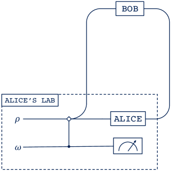
Figure 1: Indefinite causal key distribution with no eavesdroppers. A key is shared between Alice and Bob by sending a qubit $\rho$ to them in a superposition of orders controlled by the qubit $\omega$. Alice and Bob perform projective measurements randomly in either the Pauli $x$ or $z$-basis. After discarding cases in which Alice and Bob measured in different bases, they are left with identical keys. Regardless of the superposition of orderings, $\omega$ never changes when there are no eavesdroppers.

Alice and Bob then both make a random choice to measure either in the Pauli $z$-basis $\{|0\rangle,|1\rangle\}$ or $x$-basis $\{|+\rangle,|-\rangle\}$. We can therefore think of Alice and Bob as acting on the state by putting it through a quantum channel $\mathcal{A}$, defined by the Kraus operators

$$\begin{aligned} A_{0}&=\frac{1}{\sqrt{2}}|0\rangle\langle 0|,\\ A_{1}&=\frac{1}{\sqrt{2}}|1\rangle\langle 1|,\\ A_{+}&=\frac{1}{\sqrt{2}}|+\rangle\langle+|,\\ A_{-}&=\frac{1}{\sqrt{2}}|-\rangle\langle-|,\end{aligned}$$ (1)

where the factors of $1/\sqrt{2}$ arise because we are assuming Alice and Bob are both equally likely to measure in the $x$ or $z$-basis. For convenience, define the set containing the Kraus operator indices by $I:=\{0,1,+,-\}$. It should be made clear that Alice and Bob are not just putting $\rho$ through some quantum channel, they are indeed performing the stated measurements. They could, for example, store their measurement results in an ancillary register $R$ (available only in their respective laboratories) initially in the state $|0\rangle_{R}$. The corresponding Kraus operators that would achieve this would have the form $A^{\prime}_{i}=|i\rangle\langle i|\otimes|i\rangle_{R}\langle 0|_{R}/\sqrt{2}$ for $i\in I$. Having said this, since these ancillary systems factor out, we can take $A_{i}$ to have the form given in Eq. (1).

Following their measurements, Alice and Bob then publicly discuss the basis they chose for each measurement and only keep the measurement outcomes in which they measured $\rho$ in the same basis. Assuming no errors occur between Alice and Bob’s measurements, their keys, made up of the measurement outcomes they kept, should be identical. In what follows, similarly to what we discussed earlier, a measurement outcome of $0$ and $+$ will correspond to a $0$ in the key. Likewise, $1$ and $-$ correspond to a $1$ in the key.

Let’s see in more detail out what happens to the state $\rho$ when it is put through the setup in FIG. 1. Following [7], the channel that $\rho$ goes through, corresponding to a superposition of being measured by Alice first then Bob, and vice versa, is given by

$$\mathcal{S}_{\omega}(\mathcal{A},\mathcal{A})(\rho)=\sum\limits_{i,j\in I}S_{ij}\rho\otimes\omega S_{ij}^{\dagger},$$ (2)

where

$$S_{ij}=A_{i}A_{j}\otimes|0\rangle\langle 0|+A_{j}A_{i}\otimes|1\rangle\langle 1|.$$ (3)

After some algebra and index relabelling, it can be shown that Eq. (2) can be rewritten as follows:

$$\mathcal{S}_{\omega}(\mathcal{A},\mathcal{A})(\rho)=\frac{1}{4}\sum\limits_{i,j\in I}\big{(}\{A_{i},A_{j}\}\rho\{A_{i},A_{j}\}^{\dagger}\otimes\omega\\ +[A_{i},A_{j}]\rho[A_{i},A_{j}]^{\dagger}\otimes\sigma_{z}\omega\sigma_{z}\big{)}$$ (4)

where $\sigma_{z}$ is the $z$ Pauli operator.

Now, recall that, after public discussion, Alice and Bob only keep the cases in which they performed a measurement in the same basis. Therefore, following this discussion, the state becomes

$$\mathcal{S}_{\omega}(\mathcal{A},\mathcal{A})(\rho)\to\frac{1}{2}\sum\limits_{S\in B}\sum\limits_{i,j\in S}\big{(}\{A_{i},A_{j}\}\rho\{A_{i},A_{j}\}^{\dagger}\otimes\omega\\ +[A_{i},A_{j}]\rho[A_{i},A_{j}]^{\dagger}\otimes\sigma_{z}\omega\sigma_{z}\big{)}$$ (5)

where the prefactor is found by requiring normalisation and $B=\{\{0,1\},\{+,-\}\}$. Noting the form of $A_{k}$ given in Eq. (1), the terms in these sums have the following properties

$$\begin{aligned} \{A_{i},A_{j}\}&=\sqrt{2}A_{i}\delta_{ij},\\ [A_{i},A_{j}]&=0,\end{aligned}$$ (6)

for all $i,j$, where $\delta_{ij}$ is the Kronecker delta. This confirms that Alice and Bob must agree in their measurement outcomes. Overall, we have that

$$\mathcal{S}_{\omega}(\mathcal{A},\mathcal{A})(\rho)\to\sum\limits_{i\in I}A_{i}\rho A_{i}^{\dagger}\otimes\omega.$$ (7)

So, when there are no eavesdroppers present, the control qubit $\omega$ stays in its original state and this situation is ultimately no different from that when the causal order is definite. Let us introduce an eavesdropper to see what changes.

II.2 Introducing an eavesdropper

Notice that, unlike in BB84, there are two places an eavesdropper can reside (see FIG. 3). Having said this, to obtain some intuition as to how eavesdroppers change things, let us first consider introducing just a single eavesdropper, Eve, between Alice and Bob as shown in FIG. 2.

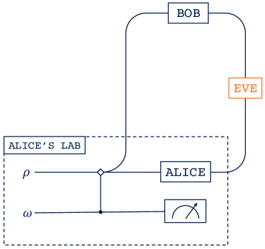
Figure 2: Indefinite causal key distribution with a single eavesdropper, Eve, between Alice and Bob.

Denote the channel corresponding to Eve’s measurement by $\mathcal{E}$, defined by the Kraus operators $\{E_{i}\}$. As before, allowing a qubit $\rho$ to be acted on by Alice, Eve and Bob in an indefinite causal order controlled by $\omega$, the channel $\rho$ passes through is given by

$$\mathcal{S}_{\omega}(\mathcal{A},\mathcal{E},\mathcal{A})(\rho)=\sum\limits_{i,j,k}S_{ijk}\rho\otimes\omega S_{ijk}^{\dagger},$$ (8)

where

$$S_{ijk}:=A_{i}E_{j}A_{k}\otimes|0\rangle\langle 0|+A_{k}E_{j}A_{i}\otimes|1\rangle\langle 1|.$$ (9)

Note that $E_{j}$ is always in the middle since Eve is in between Alice and Bob. After some algebra and index relabelling, this channel can be rewritten as

$$\mathcal{S}_{\omega}(\mathcal{A},\mathcal{E},\mathcal{A})(\rho)=\frac{1}{4}\sum\limits_{i,j,k}\big{(}\{A_{i},E_{j},A_{k}\}\rho\{A_{i},E_{j},A_{k}\}^{\dagger}\otimes\omega+[A_{i},E_{j},A_{k}]\rho[A_{i},E_{j},A_{k}]^{\dagger}\otimes\sigma_{z}\omega\sigma_{z}\big{)},$$ (10)

where

$$\{A_{i},E_{j},A_{k}\}:=A_{i}E_{j}A_{k}+A_{k}E_{j}A_{i}$$ (11)

and analogously for the commutator brackets.

After discarding the cases in which Alice and Bob measured $\rho$ in different bases,

$$\mathcal{S}_{\omega}(\mathcal{A},\mathcal{E},\mathcal{A})(\rho)\to\frac{1}{2}\sum\limits_{j}\sum\limits_{S\in B}\sum\limits_{i,k\in S}\left(\{A_{i},E_{j},A_{k}\}\rho\{A_{i},E_{j},A_{k}\}^{\dagger}\otimes\omega+[A_{i},E_{j},A_{k}]\rho[A_{i},E_{j},A_{k}]^{\dagger}\otimes\sigma_{z}\omega\sigma_{z}\right),$$ (12)

where the prefactor is once again deduced by requiring normalisation. From this, we can see that, like before, the $\omega$ terms survive. But more interestingly, notice that the $\sigma_{z}\omega\sigma_{z}$ terms can survive too. For example, suppose Alice and Bob measure in the $z$-basis and Eve measures in the $x$-basis, then it is possible for Alice to obtain an outcome of 0, and Bob an outcome of 1. This combination allows for $[A_{0},E_{\pm},A_{1}]\neq 0$.

We may therefore hypothesise that if Eve attempts to extract information about the state when in between Alice and Bob, she induces a nonzero $\sigma_{z}\omega\sigma_{z}$ term. So, if we were to let $\omega=|+\rangle\langle+|$ (and therefore $\sigma_{z}\omega\sigma_{z}=|-\rangle\langle-|$), if someone were to perform the measurement $\{|+\rangle\langle+|,|-\rangle\langle-|\}$ on the control qubit $\omega$, and obtain an outcome of $-$, they could conclude that there was an eavesdropper in between Alice and Bob. To reiterate, this differs from other QKD protocols in that no subset of the distributed key need be publicly compared and then discarded to determine the presence of Eve.

II.3 Introducing another eavesdropper

Let us now see what happens when two eavesdroppers are introduced. There being more than one eavesdropper allows for both correlated and uncorrelated strategies. Although the results derived for correlated attacks include uncorrelated ones as a special case, different mathematical tools to those used so far are required. We therefore consider the cases separately, with the bulk of the correlated case being presented in Appendix B.

II.3.1 Uncorrelated eavesdroppers

Let us begin with the uncorrelated eavesdropping scenario. For simplicity, here we assume that Alice and Bob would like their shared key to contain, on average, equal numbers of 0s and 1s. Therefore, we can make a natural choice of $\rho$ to be the maximally mixed state $\mathbbm{1}/2$, which simplifies some of our results. Having said this, we keep $\rho$ explicit for as long as we can for clarity. Now, if Alice is in the lab in which the state $\rho$ is created and entangled with $\omega$ (thereby inducing the indefinite causal order), there are two places eavesdroppers, who we call Eve and Yves, can be located. This setup is shown in FIG. 3.

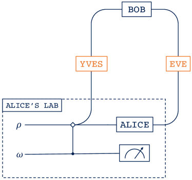
Figure 3: Indefinite causal quantum key distribution with uncorrelated eavesdroppers Eve and Yves.

Suppose Alice and Bob’s actions on $\rho$ are once again described by the channel $\mathcal{A}$ defined by the Kraus operators given in Eq. (1), and let Eve and Yves’ actions be given by the channels $\mathcal{E},\mathcal{Y}$ with Kraus operators $\{E_{i}\},\{Y_{j}\}$ respectively. Then the total channel, depicted in FIG. 3, can be defined using the Kraus operators

$$S_{ijkl}=Y_{i}A_{j}E_{k}A_{l}\otimes|0\rangle\langle 0|+A_{l}E_{k}A_{j}Y_{i}\otimes|1\rangle\langle 1|,$$ (13)

such that the state $\rho\otimes\omega$ evolves as follows:

$$\rho\otimes\omega\to\mathcal{S}_{\omega}(\mathcal{Y},\mathcal{A},\mathcal{E},\mathcal{A})(\rho)=\sum\limits_{i,j,k,l}S_{ijkl}\rho\otimes\omega S_{ijkl}^{\dagger}.$$ (14)

Defining

$$\begin{aligned} \{A,B,C,D\}&:=ABCD+DCBA,\\ [A,B,C,D]&:=ABCD-DCBA,\end{aligned}$$ (15)

notice that $S_{ijkl}$ can be rewritten as

$$S_{ijkl}=\frac{1}{2}\{Y_{i},A_{j},E_{k},A_{l}\}\otimes\mathbbm{1}+\frac{1}{2}[Y_{i},A_{j},E_{k},A_{l}]\otimes\sigma_{z}.$$ (16)

Like before, after performing their measurements, Alice and Bob have a public discussion and discard the cases in which different bases were used. So, the state $\rho\otimes\omega$ evolves as $\rho\otimes\omega\to\mathcal{S}_{\omega}(\mathcal{Y},\mathcal{A},\mathcal{E},\mathcal{A})(\rho)\to\rho_{\text{keep}}$, where

$$\rho_{\text{keep}}=\frac{1}{2}\sum\limits_{i,k}\sum\limits_{S\in B}\sum\limits_{j,l\in S}\Big{(}\{Y_{i},A_{j},E_{k},A_{l}\}\rho\{Y_{i},A_{j},E_{k},A_{l}\}^{\dagger}\otimes\omega+[Y_{i},A_{j},E_{k},A_{l}]\rho[Y_{i},A_{j},E_{k},A_{l}]^{\dagger}\otimes\sigma_{z}\omega\sigma_{z}\\ +\{Y_{i},A_{j},E_{k},A_{l}\}\rho[Y_{i},A_{j},E_{k},A_{l}]^{\dagger}\otimes\omega\sigma_{z}+[Y_{i},A_{j},E_{k},A_{l}]\rho\{Y_{i},A_{j},E_{k},A_{l}\}^{\dagger}\otimes\sigma_{z}\omega\Big{)}.$$ (17)

Note that, similarly to the case of one eavesdropper, the $\omega$ term is not the only one to appear in the final state of the system. Therefore, if these new terms are nonzero and distinguishable from the $\omega$ terms by measuring the control state, we can determine the presence of Eve and/or Yves. As was noticed before, $\omega$ and $\sigma_{z}\omega\sigma_{z}$ are perfectly distinguishable from one another if we take $\omega=|+\rangle\langle+|$.

So, taking $\omega=|+\rangle\langle+|$, performing the measurement $\{|+\rangle\langle+|,|-\rangle\langle-|\}$ allows us to detect the presence of eavesdroppers with probability

$$P_{\text{detect}}=\operatorname{\text{Tr}}(\mathbbm{1}\otimes|-\rangle\langle-|\rho_{\text{keep}}).$$ (18)

Further, noting that from here on, we will be using $\rho=\mathbbm{1}/2$, we can state the following theorem.

Theorem II.1.

When $\rho=\mathbbm{1}/2$, the presence of uncorrelated eavesdroppers can be detected with probability

$$P_{\text{detect}}=\frac{1}{2}-\frac{1}{8}\sum\limits_{i,k}\sum\limits_{S\in B}\sum\limits_{j,l\in S}(\langle l|Y_{i}|j\rangle\langle l|Y_{i}^{\dagger}|j\rangle\\ \times\langle j|E_{k}|l\rangle\langle j|E_{k}^{\dagger}|l\rangle),$$ (19)

where $B=\{\{0,1\},\{+,-\}\}$. Further, $P_{\text{detect}}=0$ if and only if, $\forall i,k$, it is true that $Y_{i}\propto E_{k}\propto A$ where $A\in\{\mathbbm{1},\sigma_{x},\sigma_{y},\sigma_{z}\}$.

This theorem is proved in Appendix A and what it is saying is that it’s only possible for uncorrelated eavesdroppers to go undetected when they don’t extract any information about the key being shared (since their Kraus operators must be proportional to unitary operators). It follows that, if Eve and/or Yves do extract information about the key, they will be detected with at least probability $P_{\text{detect}}$.

Another result of interest is the probability that Alice and Bob share the same key. This is calculated using

$$P_{\text{success}}=\operatorname{\text{Tr}}\big{(}\rho_{\text{keep}}\big{|}_{j=l}\big{)}$$ (20)

where $\rho_{\text{keep}}\big{|}_{j=l}$ denotes the terms of $\rho_{\text{keep}}$ in which Alice and Bob’s Kraus operators (and therefore measurement outcomes) agree. Again, after a little algebra, we find that

$$P_{\text{success}}=\frac{1}{8}\sum\limits_{i,k}\sum\limits_{j\in I}\langle j|\{Y_{i}^{\dagger},Y_{i}\}|j\rangle|\langle j|E_{k}|j\rangle|^{2},$$ (21)

where $I=\{0,1,+,-\}$, as in Sec. II.1.

II.3.2 Correlated eavesdroppers

So far, we have only considered Eve and Yves to be uncorrelated with one another. It turns out that when we allow them to be correlated, they still cannot learn anything useful about the key without being detected. They can, however, do a little better than in the uncorrelated case: they can find Kraus operators that tell them something, first, about which basis Alice and Bob measured in and, second, about whether each bit of Alice and Bob’s keys agree or not. As mentioned, this is not useful information as the basis choice used becomes public information and knowing whether each key bit agrees or not says nothing about the key itself. Full details of the correlated case can be found in Appendix B, where, unlike the uncorrelated case, we consider what happens when an arbitrary state $\rho$ is input rather than $\mathbbm{1}/2$. It should also be noted that the results found in the correlated picture include the uncorrelated one as a special case. Therefore, Theorem II.1 actually extends to allow for arbitrary input states $\rho$.

II.4 Eavesdropper induced errors

When thinking about errors induced by eavesdroppers, there are three cases to consider.

II.4.1 Case 1: Only possible eavesdropper is Eve

As discussed before, when we know that the only place an eavesdropper (Eve) can be situated is between Alice and Bob, if present, she allows for Alice and Bob’s measurement results to sometimes disagree. When this happens, $[A_{i},E_{j},A_{k\neq i}]\neq 0$ and therefore, when measuring the control qubit in the $x$-basis, an outcome of $-$ can occur. In fact, if the control qubit is indeed measured to be $|-\rangle\langle-|$, it is impossible for Alice and Bob to have obtained the same measurement outcome. This is because, when they do, $[A_{i},E_{j},A_{i}]=A_{i}E_{j}A_{i}-A_{i}E_{j}A_{i}=0$ which implies that the only possible outcome when measuring the control qubit is $+$. It follows that if the control qubit is measured to be $|-\rangle\langle-|$, Alice and Bob’s measurement outcomes disagree and thus, their corresponding key bit differs by a bit flip. Having said this, some of the Eve induced errors live in the $\omega$ terms, since $\{A_{i},E_{j},A_{k\neq i}\}\neq 0$ is possible. Any errors go undetected when the outcome of the control qubit measurement is $+$ but they can be suppressed using the normal information reconciliation and privacy amplification methods [16].

II.4.2 Case 2: Only possible eavesdropper is Yves

When we know that only possible location for an eavesdropper is that of Yves in FIG. 3, we can deduce that no errors will ever be induced. To see this, note that $\{Y_{i},A_{j},A_{k\neq j}\},[Y_{i},A_{j},A_{k\neq j}]=0$ regardless of what $Y_{i}$ is. It follows that the only contributing terms to $\rho_{\text{keep}}$ are those in which Alice and Bob’s measurement outcomes, and therefore key bits, are the same.

II.4.3 Case 3: Number and location of eavesdroppers unknown

Finally, when eavesdroppers could be located at either or both locations and their presence is detected, we cannot determine whether an error has been caused for a particular key bit. This follows from the previous two cases: Eve induces errors when detected but Yves does not. Since we don’t know who is there, we cannot determine whether errors have been induced or not.

II.5 Example

Let us consider a simple and symmetrical example. If Eve and/or Yves are present and perform measurements independently from one another in the $x$ or $z$-basis (choosing only one or randomly between the two), they will be detected with probability $1/8$. Note that this differs from the error rate of $1/4$ in BB84 when a similar strategy is used. This is because, as was alluded to earlier, the effects of the eavesdroppers are not solely contained in the terms used to calculate $P_{\text{detect}}$: the $\sigma_{z}\omega\sigma_{z}$ terms. Some of them lie in the $\omega,\omega\sigma_{z}$ and $\sigma_{z}\omega$ terms. It is, however, possible that a different measurement on the control qubit could result in better odds. Here, we do not attempt to optimise this measurement.

The success rate of Eve and Yves depends on which of them is present and also who’s key one, or both of them are trying to agree with. For example, maybe there’s a scenario in which Alice will only send encrypted messages to Bob, in which case Eve and/or Yves need only have the same key as Alice. As mentioned earlier, the location of the eavesdroppers also dictates the errors induced between Alice and Bob’s key. For example, if only Yves is present, there will be no errors found. If, however Eve is present, regardless of whether Yves is there or not, the probability of error in Alice and Bob’s key is 3/4, similarly to what is observed in BB84.

III Conclusion and discussion

We have shown that, with the use of indefinite causal order, it is possible to detect eavesdroppers during a QKD task without publicly comparing any subset of a shared private key between the two parties involved, Alice and Bob. We found that this could be done using a second qubit that acts as the control in inducing the indefinite causal ordering. As far as we are aware, this differs from all other QKD protocols which require a public comparison to detect eavesdroppers. In contrast to some of these other protocols, however, there are two locations eavesdroppers can reside, allowing for correlated and uncorrelated attacks. These have both been considered and it was shown that the protocol is secure regardless of whether the shared key is completely random or not.

It is natural to ask whether this protocol is physically realisable, let alone practical. The difficulties lie in that $\rho$ must go through (projective) measurement apparatuses and carry on around the loop while simultaneously doing the same in the opposite direction along the same loop. This challenge need only be considered for Alice and Bob, however: if the eavesdroppers decide they do not care about preserving the indefinite causal order, they will destroy the superposition of the two directions which would lead to $-$ outcomes being observed when measuring the control qubit, thereby indicating their presence.

Whether or not these challenges prove too great, the results of this protocol can, in theory, be simulated using linearly polarised light, a Sagnac interferometer and some polarising filters. The Sagnac interferometer creates the indefinite causal order and the polarising filters can be orientated in various different ways to correspond to each of Alice and Bob’s measurement outcomes. More details are included in Appendix C.

When it comes to practicality, consider using a Sagnac interferometer or something similar to create an indefinite causal ordering of operations. In order for the ICO to be legitimate, the coherence length of the light used must be considerably larger than the path length of the interferometer [3], perhaps indicating a limit to how practical such a protocol would be. Another limitation becomes apparent when we notice that two qubits are required to distribute one key bit securely, compared to BB84’s one qubit. Perhaps this second, control qubit could find a secondary use beyond determining the presence of eavesdroppers, but this has not considered this here.

A possible benefit to this protocol lies in the fact that it allows us to continuously monitor for eavesdroppers. This feature could perhaps find use in streaming scenarios where it’s possible an eavesdropper begins intercepting the signal part way through the distribution. To fully utilise this, it would be interesting to consider what would happen if Alice wanted to share a non-random binary string with Bob, that is, a binary string containing some information. This is possible since Alice can create $\rho$ in her lab and Theorem B.1 says that eavesdroppers will be detected regardless of $\rho$. We leave this, along with full experimental implementations for future work.

Appendix A Probability of eavesdropper detection is nonzero

Here we prove Theorem II.1, stated again for convenience:

Theorem II.1.

When $\rho=\mathbbm{1}/2$, the presence of uncorrelated eavesdroppers can be detected with probability

$$P_{\text{detect}}=\frac{1}{2}-\frac{1}{8}\sum\limits_{i,k}\sum\limits_{S\in B}\sum\limits_{j,l\in S}(\langle l|Y_{i}|j\rangle\langle l|Y_{i}^{\dagger}|j\rangle\\ \times\langle j|E_{k}|l\rangle\langle j|E_{k}^{\dagger}|l\rangle),$$ (22)

where $B=\{\{0,1\},\{+,-\}\}$. Further, $P_{\text{detect}}=0$ if and only if, $\forall i,k$, it is true that $Y_{i}\propto E_{k}\propto A$ where $A\in\{\mathbbm{1},\sigma_{x},\sigma_{y},\sigma_{z}\}$.

First, using Eq. (1), the form of $P_{\text{detect}}$ follows, after some algebra, from Eq. (18). Next, we show that Eve and Yves go undetected (that is, $P_{\text{detect}}=0$) if and only if each of their Kraus operators are all proportional to either $\mathbbm{1},\sigma_{x},\sigma_{y}$ or $\sigma_{z}$. The reverse implication can be seen to true by the fact that $P_{\text{detect}}=0$ when substituting $Y_{i},E_{k}\propto A,~{}\forall i,k$ into Eq. (19) (or Eq. (22)), where $A\in\{\mathbbm{1},\sigma_{x},\sigma_{y},\sigma_{z}\}$.

Conversely, let $P_{\text{detect}}=0$. This means that $\operatorname{\text{Tr}}(\mathbbm{1}\otimes|-\rangle\langle-|\rho_{\text{keep}})=0$ which, using Eq. (17) with $\rho=\mathbbm{1}/2$, implies that

$$\frac{1}{4}\sum\limits_{S\in B}\sum\limits_{i,k}\sum\limits_{j,l\in S}\operatorname{\text{Tr}}\big{(}[Y_{i},A_{j},E_{k},A_{l}][Y_{i},A_{j},E_{k},A_{l}]^{\dagger}\big{)}=0.$$ (23)

Notice that, since $[Y_{i},A_{j},E_{k},A_{l}][Y_{i},A_{j},E_{k},A_{l}]^{\dagger}$ is a positive operator, $\operatorname{\text{Tr}}\big{(}[Y_{i},A_{j},E_{k},A_{l}][Y_{i},A_{j},E_{k},A_{l}]^{\dagger}\big{)}=0~{}\forall i,k$ and $j,l\in S~{}\forall S\in B$. Now, for any matrix $X$, it can be shown, using the singular value decomposition, that if $\operatorname{\text{Tr}}(XX^{\dagger})=0$, then $X=0$. It therefore follows that $[Y_{i},A_{j},E_{k},A_{l}]=0~{}\forall i,k$ and $j,l\in S~{}\forall S\in B$, which implies

$$\langle j|E_{k}|l\rangle Y_{i}|j\rangle\langle l|-\langle l|E_{k}|j\rangle|l\rangle\langle j|Y_{i}=0$$ (24)

for the same options of $i,j,k,l$. In what follows, everything that is said must hold for all $i,k$.

Let us find the constraints these equations put on Eve and Yves’ channels. Since $Y_{i},E_{k}$ are assumed to be nonzero, they both must have at least one nonzero element in each basis ($x$ and $z$). Consider, first, the case in which $E_{k}$ has a nonzero diagonal element in both bases. That is, suppose that, for some $S\in B$, $\exists j,m\in S$ such that $\langle j|E_{k}|j\rangle,\langle m|HE_{k}H^{\dagger}|m\rangle\neq 0$ where $H=(\sigma_{x}+\sigma_{z})/\sqrt{2}$ is the Hadamard operator that changes between $x$ and $z$ bases. It follows that, in order for Eq. (24) to be true in this case,

$$\begin{cases}[Y_{i},|j\rangle\langle j|]=0,\\ [Y_{i},H|m\rangle\langle m|H^{\dagger}]=0\end{cases}\implies\begin{cases}[Y_{i},\sigma_{z}]=0,\\ [Y_{i},\sigma_{x}]=0\end{cases}$$ (25)

which implies that $[Y_{i},\sigma_{w}]=0~{}\forall w\in\{x,y,z\}$. Since $Y_{i}$ trivially commutes with $\mathbbm{1}$, we therefore have that $Y_{i}$ commutes with the irreducible representation of the Pauli group which has $\mathbbm{1}$ representing the identity. Thus, by Schur’s Lemma, $Y_{i}\propto\mathbbm{1}$. Now to find $E_{k}$. Using this form of $Y_{i}$ in Eq. (24), taking $a,b\in S$ for any $S\in B$ such that $a\neq b$, we have

$$\langle a|E_{k}|b\rangle|a\rangle\langle b|-\langle b|E_{k}|a\rangle|b\rangle\langle a|=0$$ (26)

which can only be true if $\langle a|E_{k}|b\rangle=\langle b|E_{k}|a\rangle=0$. Since this must hold for $a,b$ in both bases, it follows that

$$\begin{aligned} E_{k}&=\alpha|j\rangle\langle j|+\beta|l\rangle\langle l|\\ &=\gamma H|m\rangle\langle m|H^{\dagger}+\delta H|n\rangle\langle n|H^{\dagger},\end{aligned}$$ (27)

where $\alpha,\beta,\gamma,\delta\in\mathbb{C}$ and $j,l,m,n\in S$ for some $S\in B$. Using

$$H|a\rangle=\frac{1}{\sqrt{2}}\left[(-1)^{aj}|j\rangle+(-1)^{al}|l\rangle\right],$$ (28)

where we are using the shorthand $(-1)^{+}:=(-1)^{0}=1$ and $(-1)^{-}:=(-1)^{1}=-1$, this implies that $\alpha=\beta=(\gamma+\delta)/2$ and hence $E_{k}\propto\mathbbm{1}$.

Next, consider the case in which $E_{k}$ has a diagonal element in only one of the bases. That is, $\exists S\in B$, such that $\forall j\in S$, $\langle j|E_{k}|j\rangle=0$ but $\langle m|HE_{k}H^{\dagger}|m\rangle\neq 0$ for some $m\in S$. It follows that $\exists j,l\in S$ such that $\langle j|E_{k}|l\rangle\neq 0$. Similarly to before, $\langle m|HE_{k}H^{\dagger}|m\rangle\neq 0$ implies that $[Y_{i},H|m\rangle\langle m|H^{\dagger}]=0\implies[Y_{i},\sigma_{w}]=0\text{ such that }w=x\text{ if }m\in\{0,1\}\text{ and }w=z\text{ if }m\in\{+,-\}$. Therefore $Y_{i}=\alpha^{\prime}\mathbbm{1}+\beta^{\prime}\sigma_{w}$ for some $\alpha^{\prime},\beta^{\prime}\in\mathbb{C}$. So, using this form of $Y_{i}$ in Eq. (24) with $j\neq l$, we find that

$$\langle j|E_{k}|l\rangle(\alpha^{\prime}|j\rangle\langle l|+\beta^{\prime}|l\rangle\langle l|)\\ -\langle l|E_{k}|j\rangle(\alpha^{\prime}|l\rangle\langle j|+\beta^{\prime}|l\rangle\langle l|)=0.$$ (29)

Since $Y_{i}\neq 0$ and $\langle j|E_{k}|l\rangle\neq 0$, we have that $\langle l|E_{k}|j\rangle\neq 0$. So, in order for Eq. (29) to be true, $\alpha^{\prime}=0$ and $\langle j|E_{k}|l\rangle=\langle l|E_{k}|j\rangle$. Thus, $Y_{i},E_{k}\propto\sigma_{w}$, where $w$ depends on the basis that $i,j$ correspond to.

Finally, if the previously discussed cases are not true, we arrive at the scenario in which $E_{k}$ only has off-diagonal terms in both bases. That is, $\langle j|E_{k}|j\rangle=\langle m|HE_{k}H^{\dagger}|m\rangle=0~{}\forall j,m$ and $\exists j,l,m,n\in S$ for some $S\in B$ (where $l\neq j,n\neq m$) such that $\langle j|E_{k}|l\rangle,\langle m|HE_{k}H^{\dagger}|n\rangle\neq 0$. It follows that

$$\begin{aligned} E_{k}&=\alpha^{\prime\prime}|j\rangle\langle l|+\beta^{\prime\prime}|l\rangle\langle j|\\ &=\gamma^{\prime}H|m\rangle\langle n|H^{\dagger}+\delta^{\prime}H|n\rangle\langle m|H^{\dagger},\end{aligned}$$ (30)

where $\alpha^{\prime\prime},\beta^{\prime\prime},\gamma^{\prime},\delta^{\prime}\in\mathbb{C}$. Using $H$ as defined in Eq. (28), it follows that $\delta^{\prime}=-\gamma^{\prime}$ and $\alpha^{\prime\prime}=-\beta^{\prime\prime}$ which means that $E_{k}\propto\sigma_{y}$. Using this form of $E_{k}$, we have that $\langle j|E_{k}|l\rangle=-\langle l|E_{k}|j\rangle\neq 0$, which, using Eq. (24) implies that $Y_{i}|j\rangle\langle l|+|l\rangle\langle j|Y_{i}=0~{}\forall j,l\in S,\forall S\in B$. It follows that $\langle j|Y_{i}|j\rangle=0~{}\forall j,~{}\langle j|Y_{i}|l\rangle=-\langle l|Y_{i}|j\rangle~{}\forall j,l$, and therefore $Y_{i}\propto\sigma_{y}$. We conclude that an uncorrelated Eve and Yves go undetected if and only if $Y_{i},E_{k}\propto A$ $\forall i,k,$ where $A\in\{\mathbbm{1},\sigma_{x},\sigma_{y},\sigma_{z}\}$.

Appendix B Correlated eavesdroppers

Let us now consider the situation in which our eavesdroppers Eve and Yves are no longer independent, but instead can work together. In order to do this, it is convenient to use the process matrix formalism [17]. To utilise this technique, we reinterpret the Hilbert space $\mathcal{H}^{X}$ of the system passing through the labs of Alice, Bob, Eve and Yves as two spaces $\mathcal{H}^{X_{I}},\mathcal{H}^{X_{O}}$ which correspond to the Hilbert spaces of the system incoming to and outgoing from the lab $X$ respectively. We can then employ the Choi-Jamiołkowski (CJ) isomorphism which details a correspondence between completely positive (CP) maps $\mathcal{X}:\mathcal{L}(\mathcal{H}^{X_{I}})\to\mathcal{L}(\mathcal{H}^{X_{O}})$ and positive semi-definite operators $M^{X}\in\mathcal{L}(\mathcal{H}^{X_{I}})\otimes\mathcal{L}(\mathcal{H}^{X_{O}})$, where $\mathcal{L}(\mathcal{H}^{X})$ denotes the space of linear operators on $\mathcal{H}^{X}$. Explicitly,

$$M^{X}=(\mathcal{I}\otimes\mathcal{X})(|\mathbbm{1}\rangle\!\rangle^{X_{I}X_{I}^{\prime}}\langle\!\langle\mathbbm{1}|^{X_{I}X_{I}^{\prime}})$$ (31)

where $|\mathbbm{1}\rangle\!\rangle^{AB}=\sum_{j}|jj\rangle^{AB}$ with $j\in\{0,1\}$ for our purposes, and the primed superscript $X_{I}^{\prime}$ indicates that the space $\mathcal{H}^{X_{I}^{\prime}}$ is a copy of $\mathcal{H}^{X_{I}}$. The channel $\mathcal{X}$ can be recovered using

$$\mathcal{X}(\rho)=\operatorname{\text{Tr}}_{X_{I}}\!\left[(\rho^{T}\otimes\mathbbm{1})M^{X}\right]$$ (32)

for some state $\rho$, where the superscript $T$ denotes the transpose with respect to the $\{0,1\}$ basis. In general, since we require each lab to obey quantum mechanics locally, the CP maps we consider make up a quantum instrument. However, in our case, we won’t need to be this general and instead only consider completely positive trace preserving maps (CPTP maps).

For our situation, (depicted in FIG. 3) we have the labs of Alice, Bob, Eve and Yves. Further to this, and following [18, 17], we think of there being another lab $C$ that takes in the target and control qubits at the end of the process. That is, we think of this space as being composed from a target component and control component respectively: $\mathcal{H}^{C_{t}}\otimes\mathcal{H}^{C_{c}}$. Analogously to [18, 17], we use the process matrix to encode the causal structure of the setup shown in FIG. 3. If we input a pure state $\rho=|\psi\rangle\langle\psi|$ with control qubit $\omega=|+\rangle\langle+|$, the process matrix we use is $W=|w\rangle\langle w|$ where

$$|w\rangle=\frac{1}{\sqrt{2}}\big{(}|\psi\rangle^{Y_{I}}|\mathbbm{1}\rangle\!\rangle^{Y_{O}B_{I}}|\mathbbm{1}\rangle\!\rangle^{B_{O}E_{I}}|\mathbbm{1}\rangle\!\rangle^{E_{O}A_{I}}|\mathbbm{1}\rangle\!\rangle^{A_{O}C_{t}}|0\rangle^{C_{c}}+|\psi\rangle^{A_{I}}|\mathbbm{1}\rangle\!\rangle^{A_{O}E_{I}}|\mathbbm{1}\rangle\!\rangle^{E_{O}B_{I}}|\mathbbm{1}\rangle\!\rangle^{B_{O}Y_{I}}|\mathbbm{1}\rangle\!\rangle^{Y_{O}C_{t}}|1\rangle^{C_{c}}\big{)}.$$ (33)

Intuitively, the CJ isomorphism says that one can think of the temporal evolution of a state through a channel from $\mathcal{L}(\mathcal{H}^{X_{I}})$ to $\mathcal{L}(\mathcal{H}^{X_{O}})$ as a spatial teleportation of the state between the same two spaces. Therefore, we can think of the process matrix as providing the route by which $|\psi\rangle$ is teleported to $\mathcal{H}^{C_{t}}$.

Let us now write down the positive semidefinite operators that describe each lab’s channel. For Alice and Bob, being independent, these are given by

$$\begin{aligned} M^{X}&=(\mathcal{I}\otimes\mathcal{X})(|\mathbbm{1}\rangle\!\rangle^{X_{I}X_{I}^{\prime}}\langle\!\langle\mathbbm{1}|^{X_{I}X_{I}^{\prime}})\\ &=\sum\limits_{i,j,k}(|i\rangle\langle j|)^{X_{I}}\otimes(X_{k}|i\rangle\langle j|X_{k}^{\dagger})^{X_{O}},\end{aligned}$$ (34)

where $X\in\{A,B\}$ and $X_{k}\in\{A_{k},B_{k}\}$ are the Kraus operators defining the channel $\mathcal{X}\in\{\mathcal{A},\mathcal{B}\}$. Remember that Alice and Bob’s channel are the same, we just give them different labels here to make the setup clearer. Contrarily to Alice and Bob, Eve and Yves don’t necessarily act independently from one another. As shown in FIG. 4, we can think of Eve and Yves as belonging to some “superlab” (with CJ operator, channel and Kraus operators denoted using $M^{Z},\mathcal{Z},Z_{k}$ respectively) which acts on the space $\mathcal{L}(\mathcal{H}^{Y_{I}})\otimes\mathcal{L}(\mathcal{H}^{Y_{O}})\otimes\mathcal{L}(\mathcal{H}^{E_{I}})\otimes\mathcal{L}(\mathcal{H}^{E_{O}})$ using

$$M^{Z} =(\mathcal{I}^{Y_{I}E_{I}}\otimes\mathcal{Z}^{Y_{I}^{\prime}E_{I}^{\prime}})(|\mathbbm{1}\rangle\!\rangle^{Y_{I}Y_{I}^{\prime}}\langle\!\langle\mathbbm{1}|^{Y_{I}Y_{I}^{\prime}}\otimes|\mathbbm{1}\rangle\!\rangle^{E_{I}E_{I}^{\prime}}\langle\!\langle\mathbbm{1}|^{E_{I}E_{I}^{\prime}})$$ (35)

$$=\sum\limits_{i,j,k,l,m}(|ik\rangle\langle jl|)^{Y_{I}E_{I}}\otimes(Z_{m}|ik\rangle\langle jl|Z_{m}^{\dagger})^{Y_{O}E_{O}}.$$ (36)

We can gain a little intuition by observing that when Eve and Yves are independent, $Z_{m}=E_{s}\otimes Y_{t}$, where $E_{s},Y_{t}$ are the Kraus operators defining Eve and Yves’ channels respectively. In this case, $M^{Z}=M^{E}\otimes M^{Y}$ as one might expect.

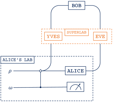
Figure 4: Indefinite causal quantum key distribution with correlated eavesdroppers Eve and Yves.

At this point, using similar logic to Eq. (32) and [17], we can find out what $\rho\otimes\omega$ becomes, when put through the setup illustrated in FIG. 4:

$$\begin{aligned} \rho\otimes\omega&\to\operatorname{\text{Tr}}_{Y_{I}Y_{O}B_{I}B_{O}E_{I}E_{O}A_{I}A_{O}}\left[(M^{Z}\otimes M^{A}\otimes M^{B}\otimes\mathbb{I}^{C_{t}C_{c}})^{T}W\right]\\ &\xrightarrow[\text{comparison}]{\text{basis}}2\sum\limits_{S\in B}\sum\limits_{i}\sum\limits_{j,k\in S}\langle\!\langle Z_{i}^{*}|\langle\!\langle A_{j}^{*}|\langle\!\langle B_{k}^{*}|(|w\rangle\langle w|)|Z_{i}^{*}\rangle\!\rangle|A_{j}^{*}\rangle\!\rangle|B_{k}^{*}\rangle\!\rangle,\end{aligned}$$ (37)

where,

$$\begin{aligned} |X_{l}^{*}\rangle\!\rangle&=(\mathbbm{1}\otimes X_{l}^{*})|\mathbbm{1}\rangle\!\rangle^{X_{I}X_{O}}=\sum\limits_{m\in\{0,1\}}|m\rangle^{X_{I}}X_{l}^{*}|m\rangle^{X_{O}},\\ |Z_{i}^{*}\rangle\!\rangle&=(\mathbb{I}\otimes Z_{i}^{*})|\mathbbm{1}\rangle\!\rangle^{Y_{I}Y_{O}}|\mathbbm{1}\rangle\!\rangle^{E_{I}E_{O}}=\sum\limits_{m,n\in\{0,1\}}|mn\rangle^{Y_{I}E_{I}}Z_{i}^{*}|mn\rangle^{Y_{O}E_{O}},\end{aligned}$$ (38)

for $X\in\{A,B\}$, $X^{*}$ indicates the complex conjugate of $X$, and the factor of 2 comes from requiring normalisation. Using these, and Eq. (33) for $W$, we can see, explicitly, that $|\psi\rangle\otimes|+\rangle$ becomes

$$\begin{aligned} |\psi\rangle\otimes|+\rangle\to&\sqrt{2}\sum\limits_{S\in B}\sum\limits_{i}\sum\limits_{j,k\in S}\langle\!\langle Z_{i}^{*}|\langle\!\langle A_{j}^{*}|\langle\!\langle B_{k}^{*}|\cdot|w\rangle\\ =&\sum\limits_{S\in B}\sum\limits_{i}\sum\limits_{j,k\in S}|f_{ijk}\rangle^{C_{t}C_{c}},\end{aligned}$$ (39)

where,

$$|f_{ijk}\rangle^{C_{t}C_{c}}=\sum\limits_{n\in\{0,1\}}\big{[}(\langle n|\otimes\mathbbm{1})(B_{k}\otimes A_{j})Z_{i}|\psi\rangle|n\rangle^{C_{t}}|0\rangle^{C_{c}}\\ +(\mathbbm{1}\otimes\langle n|)Z_{i}(B_{k}\otimes A_{j})|n\rangle^{C_{t}}|\psi\rangle|1\rangle^{C_{c}}\big{]}.$$ (40)

We can quickly check our sanity by considering the case when Eve and Yves are not present. That is, when $Z_{i}\propto\mathbbm{1}\otimes\mathbbm{1},~{}\forall i$. Here, it turns out that

$$|f_{ijk}\rangle^{C_{t}C_{c}}\propto\frac{1}{\sqrt{2}}\left(A_{j}B_{k}|\psi\rangle^{C_{t}}|0\rangle^{C_{c}}+B_{k}A_{j}|\psi\rangle^{C_{t}}|1\rangle^{C_{c}}\right)$$ (41)

which is what we’d expect from a quantum switch with two operations [3]. Similarly, if Eve and Yves act independently ($Z_{i}=E_{s}\otimes E_{t}$), $\sum_{j,k,s,t}|f_{ijk}\rangle\langle f_{ijk}|$ looks like Eq. (14).

Recall that earlier, we found that when no eavesdroppers are present, measuring the control qubit ${C_{c}}$ at the end in the $\{|\pm\rangle\}$ basis would always result in $+$. In other words, the probability of measuring $-$, denoted $P(-^{C_{c}})$ is always zero. The question now is, if a correlated Eve and Yves are present, what form must $Z_{i}$ have if $P(-^{C_{c}})=0$? And further, with this form of $Z_{i}$, can Eve and Yves extract information about the key being shared between Alice and Bob?

Theorem B.1.

For any input state, $P(-^{C_{c}})=0$ if and only if

$$Z_{i}=\sum\limits_{\mu=0}^{3}r_{i}^{\mu}\sigma_{\mu}\otimes\sigma_{\mu},$$ (42)

where $r_{i}^{\mu}\in\mathbb{C}~{}\forall\mu,i$ and $(\sigma_{0},\sigma_{1},\sigma_{2},\sigma_{3})=(\mathbbm{1},\sigma_{x},\sigma_{y},\sigma_{z})$.

Proof.

First, assume that $P(-^{C_{c}})=0$, this means that

$$\sum\limits_{S\in B}\sum\limits_{i}\sum\limits_{j,k\in S}\sum\limits_{m\in\{0,1\}}\left|(\langle m|^{C_{t}}\langle-|^{C_{c}})|f_{ijk}\rangle^{C_{t}C_{c}}\right|^{2}=0$$ (43)

which implies that $(\langle m|^{C_{t}}\langle-|^{C_{c}})|f_{ijk}\rangle^{C_{t}C_{c}}=0~{}\forall j,k\in S,S\in B,m\in\{0,1\}$ and $\forall i$. Using Eq. (40), it follows that

$$\sum\limits_{n\in\{0,1\}}(\langle n|\langle m|(B_{k}\otimes A_{j})Z_{i}|\psi\rangle|n\rangle\\ -\langle m|\langle n|Z_{i}(B_{k}\otimes A_{j})|n\rangle|\psi\rangle)=0,$$ (44)

$\forall j,k\in S,S\in B,m\in\{0,1\}\text{ and }\forall i$. Suppose we have an arbitrary, pure input state $|\psi\rangle=\alpha|0\rangle+\beta|1\rangle$, where $\alpha,\beta\in\mathbb{C}$ subject to $|\alpha|^{2}+|\beta|^{2}=1$. If we show the theorem to be true for this case, it follows that it is true for any mixed state $\rho=\sum_{\psi}p_{\psi}|\psi\rangle\langle\psi|$ by the linearity of the theory. In order to achieve this, we first of all take $|\psi\rangle\neq|0\rangle,|1\rangle$, that is, $\alpha,\beta\neq 0$.

Note that Eq. (44) must hold for both $j,k\in\{0,1\}$ and $j,k\in\{+,-\}$. Let us first see what we can find out about $Z_{i}$ when we take $j\in\{0,1\}$. In this case, Eq. (44) has the following form:

$$\delta_{jm}\left(\alpha\langle km|Z_{i}|0k\rangle+\beta\langle km|Z_{i}|1k\rangle\right)\\ =(\alpha\delta_{j0}+\beta\delta_{j1})\langle mk|Z_{i}|kj\rangle.$$ (45)

When $j\neq m$, we can quickly see that $\langle 00|Z_{i}|01\rangle,\langle 01|Z_{i}|11\rangle,\langle 10|Z_{i}|00\rangle,\langle 11|Z_{i}|10\rangle=0$. Next, when $m=j$, $Z_{i}$ is constrained by

$$\alpha\langle km|Z_{i}|0k\rangle+\beta\langle km|Z_{i}|1k\rangle=(\alpha\delta_{m0}+\beta\delta_{m1})\langle mk|Z_{i}|km\rangle.$$ (46)

When $(k,m)=(0,0),(1,1)$ we find that $\langle 00|Z_{i}|10\rangle,\langle 11|Z_{i}|01\rangle=0$ respectively. And, defining $e_{i}=\langle 10|Z_{i}|01\rangle,~{}d_{i}=\langle 01|Z_{i}|10\rangle$, when $(k,m)=(0,1)$, it turns out that $\langle 01|Z_{i}|00\rangle=\frac{\beta}{\alpha}(e_{i}-d_{i})$, and when $(k,m)=(1,0)$, $\langle 10|Z_{i}|11\rangle=\frac{\alpha}{\beta}(e_{i}-d_{i})$. Here we can see why we have not allowed $\alpha=0$ or $\beta=0$.

Taking stock so far, $Z_{i}$ has the form

$$Z_{i}=\begin{pmatrix}a_{i}&0&0&b_{i}\\ \frac{\beta}{\alpha}(e_{i}-d_{i})&c_{i}&d_{i}&0\\ 0&e_{i}&f_{i}&\frac{\alpha}{\beta}(e_{i}-d_{i})\\ g_{i}&0&0&h_{i}\end{pmatrix},$$ (47)

where all entries can be complex numbers. This can be simplified further by summing Eq. (44) over $j$ and $k$. This results in

$$\sum\limits_{n\in\{0,1\}}\langle nm|Z_{i}|\psi n\rangle=\sum\limits_{n\in\{0,1\}}\langle mn|Z_{i}|n\psi\rangle,$$ (48)

which implies

$$\sum\limits_{n\in\{0,1\}}\alpha\left(\langle nm|Z_{i}|0n\rangle-\langle mn|Z_{i}|n0\rangle\right)\\ =\sum\limits_{n\in\{0,1\}}\beta\left(\langle mn|Z_{i}|n1\rangle-\langle nm|Z_{i}|1n\rangle\right),$$ (49)

which must be true for all $m\in\{0,1\}$. Choosing $m=0$ and using Eq. (47), we find that $d_{i}=e_{i}$. So, we therefore have

$$Z_{i}=\begin{pmatrix}a_{i}&0&0&b_{i}\\ 0&c_{i}&d_{i}&0\\ 0&d_{i}&f_{i}&0\\ g_{i}&0&0&h_{i}\end{pmatrix},$$ (50)

To finish the derivation, we use the fact that Eq. (44) must also hold for $j,k\in\{+,-\}$. Using the Hadamard matrix $H=(\sigma_{x}+\sigma_{z})/\sqrt{2}=H^{\dagger}$ to relate the $x$ and $z$-bases, we replace $B_{k}\otimes A_{j}$ in Eq. (44) with $(H\otimes H)(B_{k}\otimes A_{j})(H\otimes H)$, and after some rearranging, we find that

$$\sum\limits_{n\in\{0,1\}}[\delta_{k0}+(-1)^{n}\delta_{k1}]\langle kj|(H\otimes H)Z_{i}|\psi n\rangle=\frac{1}{2}\frac{(\alpha+\beta)\delta_{j0}+(\alpha-\beta)\delta_{j1}}{\delta_{j0}+(-1)^{m}\delta_{j1}}\sum\limits_{n\in\{0,1\}}[\delta_{k0}+(-1)^{n}\delta_{k1}]\langle mn|Z_{i}(H\otimes H)|kj\rangle.$$ (51)

Straight away, we can see that the RHS has a dependence on $m$ but the LHS does not. So we can equate the $m=0$ and $m=1$ cases of the RHS. Doing this, the four cases that come from $k,j\in\{0,1\}$ result in

$$\begin{aligned} a_{i}&=h_{i},\\ g_{i}&=b_{i}+c_{i}-f_{i}.\end{aligned}$$ (52)

Updating $Z_{i}$ and looking at Eq. (51) when $(j,k,m)=(0,0,0)$ results in $c_{i}=f_{i}$ and $b_{i}=g_{i}$. Therefore we have

$$Z_{i}=\begin{pmatrix}a_{i}&0&0&b_{i}\\ 0&c_{i}&d_{i}&0\\ 0&d_{i}&c_{i}&0\\ b_{i}&0&0&a_{i}\end{pmatrix}$$ (53)

which can be rewritten as

$$Z_{i}=\frac{1}{2}\big{[}(a_{i}+c_{i})\mathbbm{1}\otimes\mathbbm{1}+(d_{i}+b_{i})\sigma_{x}\otimes\sigma_{x}\\ +(d_{i}-b_{i})\sigma_{y}\otimes\sigma_{y}+(a_{i}-c_{i})\sigma_{z}\otimes\sigma_{z}\big{]}.$$ (54)

Further, since the mapping

$$\begin{cases}r_{i}^{0}=a_{i}+c_{i},\\ r_{i}^{1}=d_{i}+b_{i},\\ r_{i}^{2}=d_{i}-b_{i},\\ r_{i}^{3}=a_{i}-c_{i}\end{cases}$$ (55)

is invertible and linear, $a_{i},b_{i},c_{i},d_{i}\in\mathbb{C}$ being independent from one another implies that $r_{i}^{\mu}\in\mathbb{C}$ are independent from one another. Therefore,

$$Z_{i}=\sum\limits_{\mu=0}^{3}r_{i}^{\mu}\sigma_{\mu}\otimes\sigma_{\mu}.$$ (56)

At this stage, one might notice that we didn’t consider all the combinations of $j,k$ in Eq. (51). It turns out that these give us no further constraints on $Z_{i}$. To confirm this, we just need to prove the reverse implication of the if and only if statement. If it turns out that we missed some constraints on $Z_{i}$, $P(-^{C_{c}})$ would be nonzero in general when using Eq. (56) for $Z_{i}$.

So, suppose that $Z_{i}$ is given by Eq. (56). Substituting this into $(\langle m|^{C_{t}}\langle-|^{C_{c}})|f_{ijk}\rangle^{C_{t}C_{c}}$ and carrying out the sum over $n$ results in

$$(\langle m|^{C_{t}}\langle-|^{C_{c}})|f_{ijk}\rangle^{C_{t}C_{c}}=\sum\limits_{\mu=0}^{3}r_{i}^{\mu}\langle m|[A_{j},\sigma_{\mu}B_{k}\sigma_{\mu}]|\psi\rangle=0$$ (57)

for all $j,k\in S,S\in B,m\in\{0,1\}$ and $\forall i$ since $[A_{j},\sigma_{\mu}B_{k}\sigma_{\mu}]=0~{}\forall j,k,\mu$.

Finally, for the cases in which $|\psi\rangle=|0/1\rangle$, notice that what we have shown so far holds for $|\psi\rangle=|+/-\rangle$. Now, the process matrix defined using Eq. (33) can equivalently be be formulated in the $x$-basis, and Alice and Bob’s measurements are invariant under this basis change. So, after converting everything to the $x$-basis, what was the situation in which $|\psi\rangle=|+/-\rangle$ becomes that of when $|\psi\rangle=|0/1\rangle$. Thus, since $Z_{i}$ has the same form when it is changed from the $z$-basis to the $x$-basis, the result also holds for this case. ∎

It is difficult to have any intuition about what Eve and Yves’ measurement would look like physically. A little can be gained, however, by considering when only one of the coefficients is nonzero for each $i$. In this case we’d have a situation similar to that considered in Sec. II.3 and Appendix A. That is, if one of Eve or Yves performs $\sigma_{i}$, then the other eavesdropper must do the same. It is possible that an ancilla qubit is necessary to understand Eve and Yves’ correlations physically: this is normally how correlations are accounted for in the process matrix formalism. The approach taken considers no physical constraints on the correlations between Eve and Yves’ and thus, operations with physical correlations should be included as a subset of those derived.

Figure 5: The results derived in this work can be simulated using polarised light to share a key between Alice and Bob, and a Sagnac interferometer to induce the indefinite causal order. Within the interferometer, polarising filters are orientated to correspond to all the valid measurement outcomes Alice and Bob obtain during the protocol.

The final question to answer is whether Eve and Yves gain any information about Alice and Bob’s shared key using Eq. (56). To do this, we calculate $P(Z_{i},A_{j},B_{k})=\langle f_{ijk}|f_{ijk}\rangle$ for $j,k\in\{0,1\}$ and $j,k\in\{+,-\}$. These are given by:

$$P(Z_{i},A_{j},B_{k})=\begin{cases}\frac{|\langle j|\psi\rangle|^{2}}{2}\!\left(|r_{i}^{0}+r_{i}^{3}|^{2}\delta_{jk}+|r_{i}^{1}+r_{i}^{2}|^{2}\delta_{j\bar{k}}\right)\!,~{}~{}j,k\in\{0,1\}\\ \frac{|\langle j|\psi\rangle|^{2}}{2}\!\left(|r_{i}^{0}+r_{i}^{1}|^{2}\delta_{jk}+|r_{i}^{2}+r_{i}^{3}|^{2}\delta_{j\bar{k}}\right)\!,~{}~{}j,k\in\{+,-\},\end{cases}$$ (58)

where $\bar{k}$ denotes “not $k$”. At first glance, it appears that Eve and Yves have access to some information about Alice and Bob’s key. However, note first that distinguishing between the two cases of $j,k\in\{0,1\}$ and $j,k\in\{+,-\}$ is of no use as Alice and Bob publicly discuss which basis they measured in after they have done so. Secondly, although Eve and Yves could alter $r_{i}^{\mu}$ however they like, the only information they could gain is about whether each bit of Alice and Bob’s key agree or not. Therefore, they can still do no better than a guess to determine the key.

Appendix C Experimental simulation

Figure 5 shows a possible experimental setup to simulate some of the results derived. The idea is to use photon polarisation (in the horizontal, vertical basis, with $|H\rangle=:|0\rangle,|V\rangle=:|1\rangle$) as the target qubit $\rho$, initially in the state $|\psi\rangle\langle\psi|$, that is acted on by Alice, Bob, Eve and Yves. As is mentioned in the main text, if we wanted Alice and Bob to have approximatly equal numbers of 0s and 1s, we can take our input state to be $\mathbbm{1}/2$. This can be achieved by taking it to be $|i\rangle$ half of the time and $|-i\rangle$ the remainder of the time. These correspond to left and right circularly polarised light respectively: $|\psi\rangle=|\pm i\rangle=(|H\rangle\pm i|V\rangle)/\sqrt{2}$. The control qubit $\omega$ is taken to be the path degree of freedom induced by a beamsplitter. Using a 50/50 beamsplitter corresponds to taking $\omega=|+\rangle\langle+|$ with $|0\rangle$ corresponding to reflection and $|1\rangle$ to transmission.

Recall that Alice and Bob perform projective measurements in either the $x$ or $z$-basis. This is difficult to do non-destructively and even more difficult to do while keeping the photon continuing around the Sagnac interferometer in its original superposition of paths. Having said this, it is possible to simulate projective measurements using polarisers. This means we can obtain the statistics that the measurements of Alice, Bob, Eve and Yves would have produced.

Explicitly, when Alice and Bob measure in the $z$-basis, we use polarisers orientated at $0$ and $\pi/2$ which correspond to measurement outcomes of 0 and 1 respectively. Likewise, when measuring in the $x$-basis, polarisers being orientated at $\pm\pi/4$ correspond to measurement outcomes of $\pm$ respectively. The probability of Alice and Bob measuring $i,j$ can be taken to be the ratio of the total intensity $I_{\text{exit}}(i,j)$ of light exiting the interferometer to that of it entering $I_{\text{enter}}$:

$$P(A_{i},B_{j})=\frac{I_{\text{exit}}(i,j)}{I_{\text{enter}}}.$$ (59)

Here, the dependence of $I_{\text{exit}}(i,j)$ on $i,j$ highlights that the interferometer is setup with Alice and Bob’s polarisers being orientated correspondingly to the measurement outcomes $i,j$ respectively. Since Alice and Bob only keep measurement results when they have publicly confirmed that they measured in the same basis, there are eight permutations when ignoring Eve and Yves. These are given in the Table 1.

Table 1:

Alice polariser orientation	Bob polariser orientation
0	0
0	$\frac{\pi}{2}$
$\frac{\pi}{2}$	0
$\frac{\pi}{2}$	$\frac{\pi}{2}$
$\frac{\pi}{4}$	$\frac{\pi}{4}$
$\frac{\pi}{4}$	$-\frac{\pi}{4}$
$-\frac{\pi}{4}$	$\frac{\pi}{4}$
$-\frac{\pi}{4}$	$-\frac{\pi}{4}$

The benefit of this protocol involves the measurement of the control qubit in the $\pm$ basis. Noticing that, after going through the main part of the Sagnac interferometer, the path that the light exits the 50/50 beamsplitter along, is controlled by the path qubit in the $\pm$ basis. That is, the $|+\rangle$ component is transmitted through the beamsplitter, whereas the $|-\rangle$ component is reflected. Therefore, placing a detector in the reflected arm corresponds to the $-$ outcome and, after a partially reflecting mirror, a detector in the transmitted arm corresponds to the $+$ outcome. The probability of measuring the eavesdroppers comes from the probability of measuring the control qubit to be $-$. Therefore, for each run of the experiment (each permutation of polariser angles), the ratio of the intensity in the $-$ arm to the total intensity exiting the interferometer is what is required. As a sanity check, this should always be zero when Eve and Yves are not present. As mentioned before, in order to exploit the features of indefinite causal order, the coherence length of the light used should be significantly longer than the path length of the interferometer. A laser can be used to achieve this.

References

- Chiribella et al. [2013] G. Chiribella, G. M. D’Ariano, P. Perinotti, and B. Valiron, Phys. Rev. A 88, 022318 (2013).
- Oreshkov et al. [2012] O. Oreshkov, F. Costa, and Č. Brukner, Nat. Commun. 3, 1092 (2012).
- Goswami et al. [2018] K. Goswami, C. Giarmatzi, M. Kewming, F. Costa, C. Branciard, J. Romero, and A. G. White, Phys. Rev. Lett. 121, 090503 (2018).
- Araújo et al. [2014] M. Araújo, F. Costa, and Č. Brukner, Phys. Rev. Lett. 113, 250402 (2014).
- Guérin et al. [2016] P. A. Guérin, A. Feix, M. Araújo, and Č. Brukner, Phys. Rev. Lett. 117, 100502 (2016).
- Zhao et al. [2020] X. Zhao, Y. Yang, and G. Chiribella, Phys. Rev. Lett. 124, 190503 (2020).
- Chiribella et al. [2021] G. Chiribella, M. Banik, S. S. Bhattacharya, T. Guha, M. Alimuddin, A. Roy, S. Saha, S. Agrawal, and G. Kar, New J. Phys. 23, 033039 (2021).
- Bennett and Brassard [1984] C. H. Bennett and G. Brassard, in Proceedings of IEEE International Conference on Computers, Systems and Signal Processing, Bangalore, India (IEEE, New York, 1984) p. 175.
- Ekert [1991] A. K. Ekert, Phys. Rev. Lett. 67, 661 (1991).
- Hwang [2003] W.-Y. Hwang, Phys. Rev. Lett. 91, 057901 (2003).
- Scarani et al. [2004] V. Scarani, A. Acin, G. Ribordy, and N. Gisin, Phys. Rev. Lett. 92, 057901 (2004).
- Koashi and Imoto [1997] M. Koashi and N. Imoto, Phys. Rev. Lett. 79, 2383 (1997).
- Scarani et al. [2009] V. Scarani, H. Bechmann-Pasquinucci, N. J. Cerf, M. Dušek, N. Lütkenhaus, and M. Peev, Rev. Mod. Phys. 81, 1301 (2009).
- Nielsen and Chuang [2002] M. A. Nielsen and I. Chuang, Quantum computation and quantum information (American Association of Physics Teachers, 2002).
- Barnett [2009] S. Barnett, Quantum information, Vol. 16 (Oxford University Press, 2009).
- Bennett et al. [1992] C. H. Bennett, F. Bessette, G. Brassard, L. Salvail, and J. Smolin, J. Cryptology 5, 3 (1992).
- Araújo et al. [2015] M. Araújo, C. Branciard, F. Costa, A. Feix, C. Giarmatzi, and Č. Brukner, New J. Phys. 17, 102001 (2015).
- Castro-Ruiz et al. [2018] E. Castro-Ruiz, F. Giacomini, and Č. Brukner, Phys. Rev. X 8, 011047 (2018).