Improved Superscaling in Quasielastic Electron Scattering with Relativistic Effective Mass
Abstract
Superscaling in electron scattering from nuclei is re-examined paying special attention to the definition of the averaged single-nucleon responses. The validity of the extrapolation of nucleon responses in the Fermi gas has been examined, which previously lacked a theoretical foundation. To address this issue, we introduce new averaged responses with a momentum distribution smeared around the Fermi surface, allowing for momenta above the Fermi momentum. This approach solves the problem of negativity in the extrapolation away from the scaling region and, at the same time, validates its use in the scaling analysis. This work has important implications for the interpretation of scaling data and contributes to the development of a more complete understanding of the scaling approach.
I Introduction
In the field of nuclear physics, understanding the behavior of atomic nuclei under various conditions is of utmost importance. One such phenomenon is the electromagnetic response of nuclei in electron scattering experiments Wes75 ; Sar93 ; Ben08 ; Bof96 ; Wal04 . More recently, neutrino experiments with accelerators have increased the interest and the need to describe the electro-weak response of the atomic nucleus Alv18 ; Mos16 ; Kat17 ; Alv14 . Electron and neutrino scattering processes are closely related, as the electromagnetic current is linked to the weak isovector current Ama20 ; Ank22 ; Ama06 . Therefore, it is of central importance to describe first the electromagnetic response, as there is an abundance of experimental data on these reactions archive ; archive2 .
In this article, we focus on the nuclear quasielastic response in electron scattering, and more specifically, on the superscaling model Don99 ; Don99a , whose basic theoretical foundations we aim to examine. One-nucleon emission is the most important contribution to the inclusive cross section in the quasielastic region, centered around , where is the energy transfer, , and is the momentum transfer to a nucleon with relativistic effective mass Ros80 ; Ser86 ; Dre89 ; Weh93 .
The widely used model of superscaling assumes factorization of the electron-nucleus scattering cross section, which is proportional to the average electron-nucleon scattering probability times a phenomenological scaling function that incorporates the nuclear structure information Alb88 ; Cen97 . Despite their limitations, such as neglecting the effects of final-state interactions and meson-exchange currents, this approach has the potential to provide an accurate description of the quasielastc electron and neutrino scattering data in the quasielastic peak region with only a few parameters: the Fermi momentum, , and the relativistic effective mass, —or the nucleon separation energy depending on the particular approach to superscaling Ama21 — as well as the phenomenological scaling function. Several methods have been employed to extract the phenomenological scaling function from experimental data. The SuSA (superscaling approach) model utilizes longitudinal response data Ama04 , additionally the SuSA-v2 uses theoretical input to construct a scaling function in the transverse channel Meg16b , while the more recent SuSAM* (superscaling approach with relativistic effective mass) model extract the scaling function directly from cross section data and incorporates medium corrections through the effective mass of the nucleon Mar17 ; Ama18 ; Rui18 . Attempts to extend the formalism to the inelastic region have also been made Ama04 ; Mai09 ; Meg16b .
Despite the success of the phenomenological SuSA and SuSAM* models in the quasielastic peak, one aspect of the theory that remains unverified is the choice of the nuclear average of the single-nucleon response. In most works, the single-nucleon response was averaged over the relativistic Fermi gas Alb88 , and then extrapolated by analytic continuation to the energy transfer region that is prohibited in the Fermi gas due to the Pauli blocking effect Ama04 ; Meg16b ; Ama18 . While this approach yield good results, extrapolating a function outside the range of validity is dangerous and needs a physical justification.
In this article, we investigate the behavior of the single-nucleon responses when averaged over a Fermi gas and extrapolated outside of the kinematic range allowed by the Pauli blocking effect. We show that as we move further away from the scaling region, the extrapolation loses its physical meaning and yields negative results for the response, which should be positive. On the other hand, we demonstrate that using extrapolation in the scaling region is appropriate because it produces results similar to those obtained by averaging the response over a nuclear momentum distribution, which does not suffer from this issue.
Our proposed framework involves a new definition of the single-nucleon response averaged over momentum space, with a momentum distribution where the Fermi surface is smeared out instead of using the sharp Fermi gas distribution. This average therefore has a theoretical justification, in contrast to the extrapolation approach Ama04 ; Meg16b ; Ama18 , and produces results that are similar to those of the traditional superscaling models. With this approach, we have a solid argument that justifies the choice of the single-nucleon response and does not suffer from the previous issues. While we will show that the use of the new averaged single-nucleon or the extrapolated one is indifferent in the scaling region, this work improves the superscaling formalism from the theoretical point of view by providing a physical justification for its use, which strengthens the applicability of such phenomenological models. Our findings have implications for the SuSA and SuSAM* model, as well as for other phenomenological models in nuclear physics.
The scheme of the paper is as follows. In Sect. 2 we present a brief review of superscaling formalism in the context of the SuSAM* approach. In sect. 3 we analyze the averaged single-nucleon responses, discuss the problems of the extrapolation, and propose a new definition. We give some details on the calculation of the single-nucleon responses in Appendix A. In sect 4 we present results of the single-nucleon cross sections and perform an updated scaling analysis of the 12C data using the new definition. In sect. 5 we discuss the results and finally in sect 6 we present our conclusions.
II Review of superscaling formalism
In this section we will briefly review the theory of the relativistic Fermi gas (RFG) response function and its connection with the theory of superscaling. The scaling variable was first introduced in ref. Alb88 . The scaling formalism was refined in subsequent works Cen97 ; Don99 ; Don99a until reaching the most up-to-date version of the SuSA-v2 model Ama20 .
The formalism in this work is an extension of the SuSA to the SuSAM* approach —based on the equations of nuclear matter interacting with a relativistic mean field (RMF) Ros80 ; Ser86 ; Dre89 ; Weh93 . The RMF model differs from the RFG mainly in that the nucleons acquire a relativistic effective mass . The on-shell energy with effective mass is defined as
| (1) |
In the RMF this is not the total energy of the nucleon, but rather, the nucleons acquire an additional positive vector energy that partly cancels the (negative) attraction energy of the scalar field. However in this work we deal with the one-particle one-hole (1p1h) response functions where the vector energy of particles and holes cancel. So the response only depends on the effective mass and the Fermi momentum.
II.1 Electromagnetic response functions
We consider the inclusive electron scattering process where an incident electron with energy scatters off a nucleus with scattering angle . The final electron energy is . The momentum transfer is and the energy transfer is , and . The cross section in plane-wave Born approximation with one photon-exchange is written
| (2) |
were is the final electron solid angle, is the Mott cross section,
| (3) |
and are the kinematic factors
| (4) |
and finally, , , are the longitudinal and transverse response functions defined below.
We focus on the description of the nuclear response functions resulting from the interaction of the electron with the one-body electromagnetic current, giving rise to 1p1h excitation of the Fermi gas. They are defined in a similar way to the usual RFG formalism Ama20 , with the difference that in our case the nucleons have an effective mass . The hole momentum is with and on-shell energy . By momentum conservation, the particle momentum is with on-shell energy . Pauli blocking implies . The nuclear response functions are then given by
| (5) |
where are the single-nucleon responses for the 1p1h excitation
| (6) |
corresponding to the single-nucleon hadronic tensor
| (7) |
and is the electromagnetic current matrix element
| (8) |
where and , are the Dirac and Pauli form factors of the nucleon. Note that we use the current operator in the vacuum, but the spinors correspond to nucleons with effective mass .
To compute the integral (5), we use the variables , with Jacobian . Then the integral over is made using the Dirac delta. This fixes the angle between and to the value
| (9) |
and the integration over the azimuth angle gives by symmetry of the responses when is on the -axis Ama20 . We are left with an integral over the initial nucleon energy
| (10) |
where is the initial nucleon energy in units of , and is the (relativistic) Fermi energy in the same units. Moreover we have introduced the energy distribution of the Fermi gas . The lower limit, of the integral in Eq. (10) corresponds to the minimum energy for a initial nucleon that absorbs energy and momentum . It can be written as (see Appendix C of ref. Ama20 )
| (11) |
where we have introduced the dimensionless variables
| (12) |
II.2 Geometrical interpretation
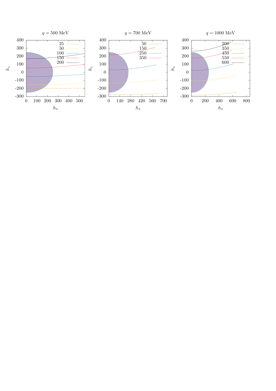
For a fixed value of , the integral over energy in Eq. (10) corresponds to integrating the single nucleon response over a path in the momentum space of the hole , weighted with the momentum distribution. This curve is easily obtained from Eq. (9), giving the angle as a function of the hole energy. Some examples are shown in Fig. 1 for three values of . For each we plot the integration trajectories in the -plane for several values of . The semicircles indicate the moment distribution for MeV. The nuclear response function, , therefore correspond to the sum (the integral) of the single-nucleon responses along one path. The minimum momentum , and therefore the minimum energy , correspond to the intersection of each curve with the axis. The curves for different values of do not intersect. The case only occurs for a certain value of , which is precisely the position of the quasielastic peak; this corresponds also to (or for the scaling variable, see below). For very large or very small -values, the curves lie in the region where the momentum distribution is zero, and therefore the corresponding response function is also zero.
Now we define a mean value of the single-nucleon responses by averaging with the energy distribution
| (13) |
This corresponds to the average of the single-nucleon response over one of the paths in Fig. 1. Using these averaged single-nucleon responses we can rewrite Eq. (10) in the form
| (14) |
This last integral depends on the variable , which in turn depends on .
II.3 Scaling
In the super-scaling approach the -scaling variable is used instead of the minimum energy of the nucleon, . This energy is transformed by a change of variable into the scaling variable, , defined as
| (15) |
where is negative (positive) for ().
The superscaling function is defined as
| (16) |
where is the kinetic Fermi energy in units of . The definition (16) is, except for a factor, similar to that of the -scaling function Sar93 ; Wes75 , where the scaling variable was the minimum moment of the initial nucleon.
In RFG and nuclear matter with RMF Eq. (16) is easily evaluated (remember that the RFG is recovered as the particular case ) as
| (17) |
Therefore the scaling function of nuclear matter is
| (18) |
Note that the scaling function of nuclear matter is zero for , and this is equivalent to . This is a consequence of the maximum momentum for the nucleons in nuclear matter, which implies that .
Using for nuclear matter we can write the response functions (14) as
| (19) |
where we have added the contribution of protons and neutrons to the response functions, and .
II.4 SuSAM*
The SuSAM* approach extends the formula (19) by replacing by a phenomenological scaling function obtained from experimental data of . In a real, finite nucleus the momentum is not limited by (in particular correlated nucleons can greatly exceed the Fermi momentum). This has the effect that the phenomenological superscaling function is not zero for , and therefore takes into account that the nucleons are not limited by a maximum Fermi momentum.
Several approaches have been used in the past to obtain a phenomenological scaling function. In the original SuSA model, based on the RFG without effective mass, the scaling function was obtained from the longitudinal response data. In the SuSAv2 model, a scaling function for the transverse response was also introduced by means of a RMF theoretical model in finite nuclei. In this paper we will focus on the SuSAM* model with effective mass where the phenomenological scaling function is obtained directly from the quasielastic data of the inclusive cross section. Different scaling models with effective mass and without effective mass provide different scaling functions, but all may reproduce the quasielastic cross section reasonably well, since they have been fitted to experimental data.
In the procedure followed in ref Mar17 ; Ama18 ; Rui18 the inclusive cross section data are divided by the contribution of the single nucleon.
| (20) |
where
| (21) |
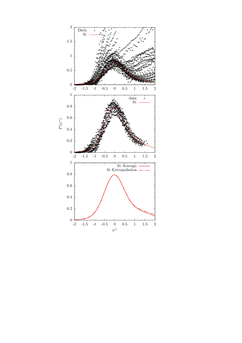
In Fig. 2 these experimental data, , are plotted against in the interval , which we call the quasielastic scaling region in this work. It is observed that about half of them roughly collapse forming a thin band around the quasielastic peak. This band constitutes the set of selected data that can be considered QE and we reject the rest, which mainly contribute to inelastic processes. The selected quasielastic data are well parameterized with a sum of two Gaussians, thus obtaining the phenomenological quasielastic function , shown also in Fig. 2.
The SuSAM* model was extended in refs. Mar21 ; Mar21b , by subtracting the theoretical contribution of the meson-exchange currents (MEC) in the 2p2h channel from the experimental data before dividing by the single nucleon, that is
| (22) |
The resulting SuSAM*+MEC model provided a somewhat smaller scaling function. However in this work we use the scaling function (20) without subtraction of MEC, since our focus will be on the average single nucleon responses. Both models give similar results for the quasielastic cross section and we do not want to complicate the calculation by introducing the 2p2h contribution, that is not relevant for our further discussion.
III Averaged single-nucleon response functions
One of the most confusing aspects in the superscaling formalism is the definition and meaning of the averaged single-nucleon response functions for or, equivalently, , i.e., outside the allowed -range of the Fermi gas. One of the goals of this paper is to shed light on this matter. Traditionally an extrapolation of the Fermi gas formula has often been used. In this section we expose the intrinsic theoretical problems of the Fermi gas extrapolation, and propose an alternative definition that is more satisfactory from the theoretical point of view.
III.1 RFG extrapolation
In the traditional superscaling approach, first the averaged single-nucleon responses are calculated for (or ) using the Fermi gas momentum distribution,
| (23) | |||||
Note that this expression is only defined for , in which case the step functions cancel and we obtain
| (24) |
The function inside the integral is well defined and positive only if , because it corresponds to the response of a single nucleon with energy , that absorbs momentum and energy . In the traditional SuSA and SuSAM* approaches the function (24) is extended analytically for in the obvious way. This is called in this work the extrapolated single nucleon response function, and it can be written equivalently in the way
| (25) |
From this expression it is clear that,for , the function inside the integral must be evaluated for . But this is not possible for a nucleon on-shell that absorbs , because its minimum energy is . Therefore it is not guaranteed that the function inside the integral is positive if is evaluated for . This is a fundamental problem of the single nucleon extrapolation. Next we will study some particular cases where the extrapolated responses are explicitly negative for , that is, for .
III.2 Longitudinal single-nucleon response
We use the analytical formulas of the single nucleon responses from Appendix A.
| (26) |
To better understand the kinematic dependence of this response function it is convenient to express it in terms of the minimal nucleon energy using
| (27) |
in the regime without Pauli blocking. Then Eq. (42) becomes
| (28) |
In this equation it is evident that the electric term is always positive. However the magnetic term is positive only for . For this reason, if is calculated using the Fermi gas momentum distribution and then extrapolated to values (or ), the magnetic term becomes negative. This does not make physical sense because the longitudinal response must be positive, by definition, regardless of the value of the form factors. In fact if we artificially turn off the electric contribution, a negative averaged response is obtained for . Let suppose for simplicity that . Then the extrapolated single-nucleon longitudinal response would be
| (29) |
that is negative for .
III.3 Transverse single-nucleon response
We find a similar situation in the case of the transverse response from Eq. (47) in the Appendix A
| (30) |
Again we can rewrite this response as a function of the minimum nucleon energy, , using
| (31) |
Rearranging terms containing and the single-nucleon transverse response becomes finally
| (32) |
Written in this way, it is evident that the magnetic contribution of is always positive. While the electrical term is positive only for . The situation is similar to what we found with the longitudinal response, but in the transverse response it is the electrical term that becomes negative in the extrapolation to . We now turn off the magnetic contribution and suppose that . Then the averaged T response in RFG would be, with analogy to Eq. (29)
| (33) |
From this expression it is clear that the extrapolated is negative for because the function inside the integral is negative, which is not physically acceptable: the transverse response should be positive by definition regardless of the form factors values. In other words, the electrical contribution to the transverse response, although samll, cannot be negative.
III.4 Alternative to the extrapolated single-nucleon responses
In this work we propose an alternative definition of the averaged single-nucleon responses that solves the extrapolation problem in the superscaling model. As we have seen, the problem is a consequence of the fact that in the Fermi gas there is a maximum momentum for the nucleons. If this momentum is exceeded by extrapolation, i.e. , mathematically this is equivalent to assuming nucleons with energy less than , which is impossible in the Fermi gas because nucleons are on-shell. Hence results without physical sense, such as negative responses, are obtained if the extrapolated formula is applied.
The proposed solution involves using equation (13) for the averaged single-nucleon responses, but introducing a momentum distribution without a maximum momentum, and that at the same time does not differ much from the Fermi gas distribution, for . An appropriate function is a distribution of Fermi type
| (34) |
Where is a smearing parameter for the Fermi surface, which is no longer restricted to a sphere as in figure 1. Then the integrals by averaging in Eq. (13) extend to infinity and therefore there is no longer an upper limit for , which can take any value up to infinity. The single-nucleon responses of the integrand always are evaluated for and they are therefore positive definite (see eqs. (28,32)).
Besides, for , the momentum distribution is similar to the Fermi Gas distribution, , and then it is expected that the averaged single-nucleon be similar to that of the RFG (see Fig.1). Now, for the integration (13) extends in momentum space along one of the paths outside the Fermi sphere of Fig. 1. Then the average has the physical sense of coming from regions above the Fermi sphere, that is to say, from the high momentum zone that the Fermi gas cannot describe. This is in accordance with the meaning attached to the experimental scaling function for , which comes mainly from high momentum nucleons.
IV Results
In this section we present results for the averaged nucleon responses and for the total nuclear responses in the SuSAM* model. The calculations are made for electron scattering off the nucleus 12C with Fermi momentum MeV/c and effective mass . These values were fitted to the quasielastic data of to obtain the best possible scaling Mar17 ; Ama18 . We evaluate the validity of the scaling model when using the Fermi gas extrapolation for the nucleon response function. Specifically, the results obtained by averaging the single-nucleon response function over a smeared Fermi momentum distribution, Eq. (34) are compared with the extrapolated response function obtained from the Fermi gas model.
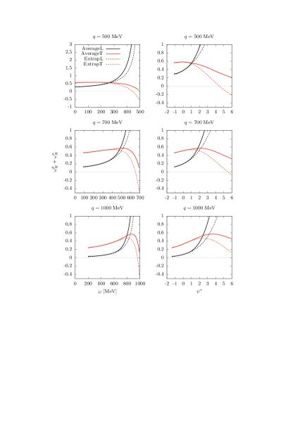
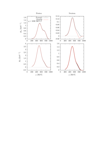
In Fig. 3 we compare the averaged nucleon responses with the extrapolated ones. The sum of proton plus neutron is shown. The averaged responses have been calculated with a Fermi distribution using a smearing parameter MeV/c. The responses do not depend much on the precise value of this parameter for small variations. We see that the averaged responses are practically the same as the extrapolated responses of the Fermi gas in the quasielastic scaling region, ,. But both results start to diverge for large or . The extrapolated transverse response becomes negative for , 5 and 7, for , 700, and 1000 MeV/c, respectively, very close to the photon line. This is easily explained because in Eq. (32) the magnetic term is multiplied by . Therefore the response is dominated by the electric term for , that is, for large , and in Eq. (33) we have seen that this term is negative when extrapolated to .
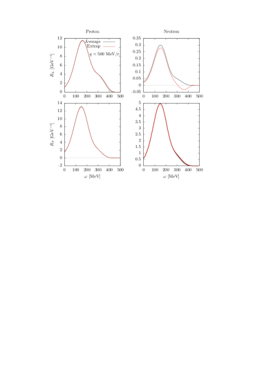
More details can be seen in Fig. 4 where we show the averaged and extrapolated response functions separated for protons and neutrons, as a function of the scaling variable. The extrapolated and averaged responses start to differ in the region and the discrepancy increases with . The extrapolated longitudinal response of neutrons is negative for . This agrees with what was seen analytically in the previous section, because the extrapolation of the longitudinal magnetic response is negative and the electric form factor of the neutron is negligible. This does not affect the results of the SuSAM* model in the scaling region because the longitudinal response of the neutron is much smaller than that of the proton.

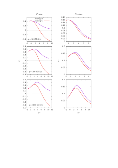
In fig. 4 we also can see see that the averaged proton transverse response is very similar to the extrapolation in the scaling region and differ for . They also start to differ in the -negative region for . The extrapolated transverse response of protons is negative from –6 depending on the value of . Again this is because the electrical term of the proton dominates this response for large since the magnetic term carries a factor , which tends to zero for . In contrast the averaged proton transverse responses are always positive.
The averaged transverse neutron response shown in Fig. 4 is similar in shape to the Fermi gas extrapolation in the scaling region. But again they differ for , where the averaged one is the largest, and the difference between the two increases with the momentum transfer.

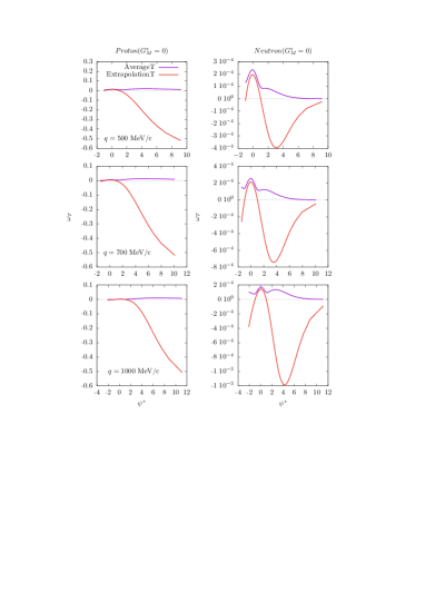
We have seen in the extrapolation formulas, Eqs. (29,33), that the magnetic contribution to the longitudinal response and the electrical contribution to the transverse response become both negative for , This can be explicitly seen in the results in Fig. 5, where we plot the longitudinal responses computed for and the transverse responses computed for , for protons and neutrons. In fact, in all cases of Fig. 5 the extrapolated responses are negative for . On the contrary the averaged responses are always positive.
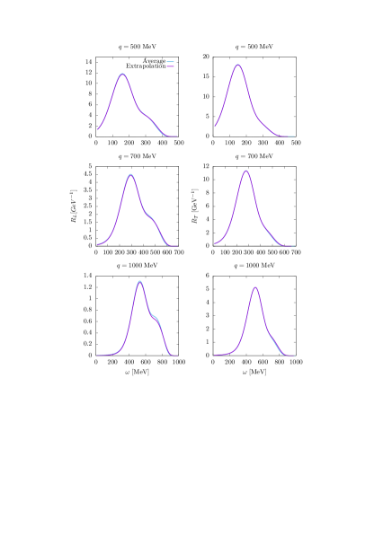
In fig 6 we use the superscaling model to investigate the nuclear responses under various inputs for the single-nucleon. The nuclear response is computed from the product of the averaged nucleon-responses and a phenomenological scaling function obtained from the data, using Eq. (19).
The results in Fig. 6 demonstrate that there are no significant differences in the separate responses of protons and neutrons when computed with the averaged single-nucleon compared to the extrapolation. The only difference is seen in the longitudinal neutron response for high , which becomes negative in the extrapolated model. However this is not relevant for the total nuclear response, as the neutron contribution is negligible in the longitudinal response as compared to the proton one.
This is verified in the results of Fig. 7 for the total responses. Both the averaged and the extrapolated single-nucleon responses give essentially the same result. The results obtained have two important implications. Firstly, they provide support for the validity of using the single-nucleon response extrapolated from the Fermi gas, as this approach yields the same results as using a response averaged with a nuclear momentum distribution that does not have a maximum momentum. Secondly, they justify the use of the averaged response as a means of avoiding the potential issues that we have identified with the extrapolation method.
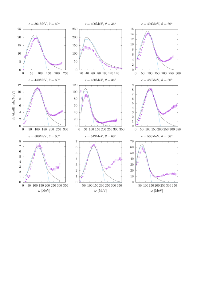
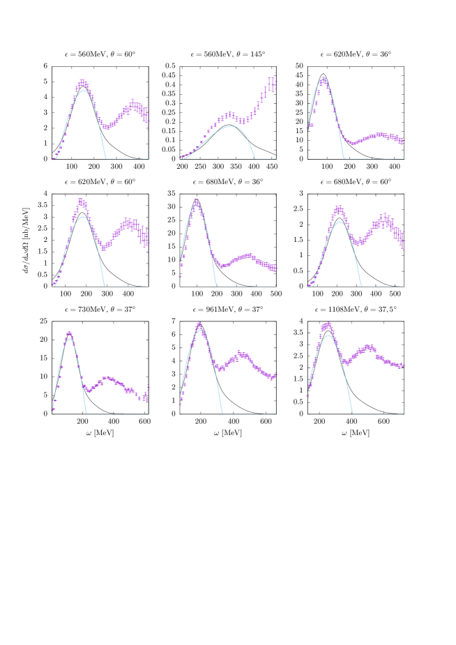
Finally we have conducted a new scaling analysis of the data using the single-nucleon response averaged with the Fermi distribution. The results, as shown in Figure 2, demonstrate that the scaling function obtained using this approach is virtually indistinguishable from the one obtained through extrapolation. These findings highlight the robustness of the scaling approach and suggest that using the averaged response may be a viable alternative to extrapolation in certain cases. Furthermore, in Figures 8 and 9, we compare the cross-section of 12C using the SuSAM* model and the RMF model of nuclear matter for a selected set of kinematics. The SuSAM* model still proves to be an excellent method to parameterize the quasielastic cross-section through a single scaling function.
V Discussion
The findings of the results section demonstrate the robustness and versatility of the superscaling models with respect to the choice of the averaged single-responses, and its potential applications in a variety of situations in electron and neutrino scattering. The updated single-nucleon responses provide a well-defined theoretical basis for the scaling function that is compatible with the traditional extrapolation in the scaling region. This reinforces the universality of the scaling function because it is independent of the way in which the average response of the nucleon is defined. This means that the scaling function can be used to describe the electromagnetic response of nucleons in different types of nuclei, regardless of their size or composition.
The averaged single-nucleon model has promising applications in other situations outside the scaling region for high-energy transfer. For instance in two-particle emission reactions, two-particle two-hole (2p2h) excitation can be produced by the one-body current due to nuclear short-range correlations. The electromagnetic interaction with a nucleon belonging to a correlated pair can result in the emission of both nucleons because the correlated nucleons acquire high-momentum components that allow the overlap of the wave function with states above the Fermi momentum. A simple model of emission of two correlated nucleons has been proposed in ref. Mar22 to explain phenomenologically the tail of the scaling function at high energies. The probability of emission of a proton-neutron pair is approximated by a factorized model, similar to the scaling approach. One factor is the sum of the averaged proton and neutron responses considered in this work. The other factor is the probability of emitting two particles while conserving energy and momentum, assumed to be proportional to the phase space of two particles in the Fermi gas. The total response is assumed to be the product of these two factors with an additional correlation factor that accounts for the average probability of the high momentum proton-neutron correlated pair. The factor is obtained phenomenologically by fitting the tail of the scaling function. In such 2p2h correlation model the contribution of the single nucleon for high outside of the scaling region plays an important role, and the extrapolation of the Fermi gas single-nucleon model is not appropriate.
Another direct application of this method concerns the calculation of the contribution of meson-exchange currents (MEC) to the quasielastic 1p1h response in the superscaling model. This calculation was performed in the RFG for instance in Refs. Ama01 ; Ama03 and involves computing an effective one-body current as the sum of one-body plus MEC, 1p1h matrix elements. The traditional scaling model with extrapolation is not trivial to apply in this case, as the single-nucleon responses of the MEC must be computed numerically. However, the averaged single-nucleon responses of the OB+MEC operator can be directly computed as we have done in this work.
VI Conclusions
In this work, we have re-examined the scaling formalism from a theoretical standpoint, with a particular emphasis on the definition of the averaged electron-nucleon responses, which are assumed to factorize in the model. Within the SuSAM* model, which takes into account the relativistic mean field through the effective mass of the nucleon, we have investigated the validity of the traditional approach of extrapolating to the single-nucleon responses averaged over the Fermi gas. A detailed analysis shows that that, for , the extrapolation formulas produce nonphysical negative results for the responses in some particular cases, which contradict the physical expectation that the response functions should always be positive. Specifically, the magnetic contribution of the longitudinal response and the electrical contribution of the transverse response become negative for . This is propagated to the total responses, resulting in the extrapolated single-nucleon transverse response becoming negative for very high values of .
Therefore we have proposed a different definition for the averaged single-nucleon responses with a smeared momentum distribution around the Fermi surface. This approach does not suffer from the problems associated with the extrapolation method, and on the other hand produces results that are similar to those of the extrapolated SuSAM* model. Our proposed approach, which takes into account the high-momentum nucleons to a certain extent, does not depend significantly on the fine details of the nuclear density due to the averaging procedure.
Despite the theoretical problems with extrapolation, in this work, we have shown that the extrapolated model produces results similar to the correctly averaged model within the scaling region . In conclusion, we have provided a solid basis for the traditional superscaling model in the quasielastic peak region. The new physically motivated definition of the averaged single-nucleon responses strengthens the physical interpretation of the superscaling model for understanding the response of atomic nuclei in electron and neutrino scattering experiments. The new method has other applications as well, for example, it allows for the inclusion of the MEC effect in the superscaling model. A calculation of this type will be presented in the future, demonstrating the versatility and potential of this new approach.
VII Acknowledgments
Work supported by: Grant PID2020-114767GB-I00 funded by MCIN/ AEI/ 10.13039/ 501100011033; FEDER/Junta de Andalucia-Consejeria de Transformacion Economica, Industria, Conocimiento y Universidades/A-FQM-390-UGR20; and Junta de Andalucia (Grant No. FQM-225).
Appendix A Single nucleon responses
The single-nucleon hadronic tensor is computed performing the spin traces (7) with the current matrix elements (8), and can be written as
| (35) |
where we have defined the four-vector , and is the initial nucleon four-momentum with effective mass . The four-momentum of the final nucleon is . The nucleon structure functions are given by
| (36) | |||||
| (37) |
where the electric and magnetic form factors for nucleons with effective mass are Ama15
| (38) |
For the form factors of the nucleon, we use the Galster parametrizations Gal71 .
Note that and are positive and depend only on . Here we compute the longitudinal and transverse components of the hadronic tensor, and respectively, appearing in inclusive electron scattering.
Longitudinal single-nucleon response
We use the following results for the time components of the basic tensors and vectors in terms of adimensional variables,
| (39) |
| (40) |
Substituting the values of these time components and of the structure functions in the hadronic tensor (35), the longitudinal single-nucleon response function becomes
| (41) |
Rearranging terms containing and this becomes
| (42) |
Transverse single-nucleon response
In the case of the transverse response and , for , where we have defined the three-vector . Then the T response is
| (43) |
Note that . The value of is the projection of the vector over the direction, which is determined by energy-momentum conservation. In fact, using Eq (9)
| (44) |
Then we have
| (45) |
Expanding the square and using , this gives gives
| (46) |
Inserting this result in Eq. (43) and using the values of from Eqs. (36,37), the transverse response becomes
| (47) |
References
- (1) G. B. West, Phys. Rept. 18, 263-323 (1975)
- (2) A. M. Saruis, Phys. Rept. 235, 57-188 (1993)
- (3) O. Benhar, D. Day, and I. Sick, Rev. Mod. Phys. 80, 189 (2008).
- (4) ] S. Boffi, C. Giusti, F. d. Pacati, and M. Radici, Electromagnetic Response of Atomic Nuclei, Oxford Studies in Nuclear Physics, Vol. 20. 20 (Clarendon Press, Oxford UK, 1996).
- (5) J. D. Walecka, Theoretical Nuclear And Subnuclear Physics (Editorial World Scientific Pub. Co. Inc., 2004).
- (6) L. Alvarez-Ruso et al., Progress in Particle and Nuclear Physics 100, 1 (2018).
- (7) U. Mosel, Ann. Rev. Nuc. Part. Sci. 66 (2016), 171.
- (8) T. Katori and M. Martini, J. Phys. G 45 (2018) no.1, 013001.
- (9) L. Alvarez-Ruso, Y. Hayato, J. Nieves, New J. Phys. 16 (2014) 075015.
- (10) J. E. Amaro, M. B. Barbaro, J. A. Caballero, R. González-Jiménez, G. D. Megias and I. Ruiz Simo, J. Phys. G 47 (2020) no.12, 124001
- (11) A. M. Ankowski, A. Ashkenazi, S. Bacca, J. L. Barrow, M. Betancourt, A. Bodek, M. E. Christy, L. D. S. Dytman, A. Friedland and O. Hen, et al. [arXiv:2203.06853 [hep-ex]].
- (12) J. E. Amaro, M. B. Barbaro, J. A. Caballero and T. W. Donnelly, Phys. Rev. Lett. 98, 242501 (2007)
- (13) O. Benhar, D. Day and I. Sick, arXiv:nucl-ex/0603032.
- (14) O. Benhar, D. Day, and I. Sick, http://faculty.virginia.edu/qes-archive/
- (15) T. W. Donnelly and I. Sick, Phys. Rev. Lett. 82, 3212-3215 (1999)
- (16) T. W. Donnelly and I. Sick, Phys. Rev. C 60, 065502 (1999)
- (17) R. Rosenfelder, Ann. Phys. (N.Y.) 128, 188 (1980).
- (18) B.D. Serot, and J.D. Walecka, Adv. Nucl. Phys. 16 (1986) 1.
- (19) D Drechselt and M M Giannini, Rep. Prog. Phys. 52 (1989) 1083.
- (20) K. Wehrberger, Phys. Rep. 225 (1993) 273.
- (21) W. M. Alberico, A. Molinari, T. W. Donnelly, E. L. Kronenberg and J. W. Van Orden, Phys. Rev. C 38, 1801-1810 (1988)
- (22) R. Cenni, T. W. Donnelly and A. Molinari, Phys. Rev. C 56, 276-291 (1997)
- (23) J. E. Amaro, M. B. Barbaro, J. A. Caballero, T. W. Donnelly, R. Gonzalez-Jimenez, G. D. Megias and I. R. Simo, Eur. Phys. J. ST 230, no.24, 4321-4338 (2021)
- (24) J. E. Amaro, M. B. Barbaro, J. A. Caballero, T. W. Donnelly, A. Molinari and I. Sick, Phys. Rev. C 71, 015501 (2005)
- (25) G. D. Megias, J. E. Amaro, M. B. Barbaro, J. A. Caballero and T. W. Donnelly, Phys. Rev. D 94, 013012 (2016).
- (26) V. L. Martinez-Consentino, I. Ruiz Simo, J. E. Amaro and E. Ruiz Arriola, Phys. Rev. C 96, no. 6, 064612 (2017).
- (27) J. E. Amaro, V. L. Martinez-Consentino, E. Ruiz Arriola and I. Ruiz Simo, Phys. Rev. C 98 (2018) 024627
- (28) I. Ruiz Simo, V. L. Martinez-Consentino, J. E. Amaro and E. Ruiz Arriola, Phys. Rev. D 97, 116006 (2018).
- (29) C. Maieron, J. E. Amaro, M. B. Barbaro, J. A. Caballero, T. W. Donnelly and C. F. Williamson, Phys. Rev. C 80, 035504 (2009)
- (30) V. L. Martinez-Consentino, I. R. Simo and J. E. Amaro, Phys. Rev. C 104, no.2, 025501 (2021)
- (31) V. L. Martinez-Consentino, J. E. Amaro and I. Ruiz Simo, Phys. Rev. D 104, no.11, 113006 (2021)
- (32) J. E. Amaro, E. Ruiz Arriola and I. Ruiz Simo, Phys. Rev. C 92, no.5, 054607 (2015) [erratum: Phys. Rev. C 100, no.1, 019904 (2019)]
- (33) S. Galster, H. Klein, J. Moritz, K. H. Schmidt, D. Wegener and J. Bleckwenn, Nucl. Phys. B 32, 221 (1971).
- (34) V. L. Martinez-Consentino, J. E. Amaro, P. R. Casale and I. Ruiz Simo, [arXiv:2210.09982 [nucl-th]].
- (35) J. E. Amaro, M. B. Barbaro, J. A. Caballero, T. W. Donnelly and A. Molinari, Nucl. Phys. A 697, 388-428 (2002)
- (36) J. E. Amaro, M. B. Barbaro, J. A. Caballero, T. W. Donnelly and A. Molinari, Nucl. Phys. A 723, 181-204 (2003)