A nearly optimal explicitly-sparse representation for oscillatory kernels with curvelet-like functions

Abstract

A nearly optimal explicitly-sparse representation for oscillatory kernels is presented in this work by developing a curvelet based method. Multilevel curvelet-like functions are constructed as the transform of the original nodal basis. Then the system matrix in a new non-standard form is derived with respect to the curvelet basis, which would be nearly optimally sparse due to the directional low rank property of the oscillatory kernel. Its sparsity is further enhanced via a-posteriori compression. Finally its nearly optimial log-linear computational complexity with controllable accuracy is demonstrated with numerical results. This explicitly-sparse representation is expected to lay ground to future work related to fast direct solvers and effective preconditioners for high frequency problems. It may also be viewed as the generalization of wavelet based methods to high frequency cases, and used as a new wideband fast algorithm for wave problems.

1 Introduction

In this work, $N$-body problems like

$$f_{i}=\sum_{j=1}^{N}K(\bm{x}_{i},\bm{y}_{j})\sigma_{j},\quad\text{for }i=1,2,,,N$$ (1)

with the oscillatory kernel being

$$K(\bm{x},\bm{y})=\frac{\text{e}^{\mathrm{i}\kappa r}}{4\pi r},\quad r=\left|\bm{x}-\bm{y}\right|$$ (2)

or its derivatives are concerned. Such computations may come from acoustic, electromagnetic, or elastodynamic problems when solved with boundary integral equations or the Lippmann-Schwinger equation [1, 2, 3, 4, 5, 6].

Two major difficulties may be encountered when solving large scale cases. Firstly, the direct evaluation is prohibitive, since its computational complexity is $O(N^{2})$ due to its densely populated system matrix. Secondly, iterative solvers which are generally used often suffer from the bad conditioning of the system matrix, especially in cases with highly oscillatory kernels [6, 7, 8, 9]. These difficulties can be overcome by constructing approximate sparse representations for the system matrix and its inverse.

Data-sparse representations for the system matrix are constructed in many fast algorithms, that is, the system is represented in a low rank factorization form with only $O(N\log^{\alpha}N)_{\alpha\geq 0}$ elements. For low frequency or even non-oscillatory cases which are mainly concerned in early research, the kernel $K(\bm{x},\bm{y})$ is asymptotically smooth when $\bm{x}$ lies far away from $\bm{y}$. Therefore, $K(\bm{x},\bm{y})$ can be approximated by a low-order expansion, and low rank approximations for off-diagonal matrix blocks corresponding to far-field interactions can be constructed. Representative fast algorithms following this idea include the fast multipole method (FMM) and its variants [10, 11, 12, 13], treecode algorithm [14], $\mathcal{H}^{2}$-matrix [15], adaptive cross approximation [16], and nested cross approximation [17, 18], etc. One of the main differences between these algorithms is that they use different functions in the low-order expansion of the kernel, or different algebraic schemes in deriving the low rank approximation for matrix blocks. Each of them can achieve a data-sparse representation for the system matrix with only $O(N)$ elements, and bring down the computational complexity to linear for low frequency cases.

For high frequency cases, however, data-sparse representations cannot be obtained by these early fast algorithms, since the approximate rank of the matrix block increases with its size [19]. Thus other mathematical properties of the kernel should be considered to develop fast algorithms. It is noticed that when the kernel is approximated with exponential expansions, the translation matrices in FMM can be diagonalized even in high frequency, thus far field interactions can be computed efficiently. This leads to the diagonal form FMM [20, 21] and high frequency FMM [22, 23]. To overcome its possible numerical instability in low frequency cases [24, 25], the wideband FMM is developed [26, 27], which is essentially the hybrid of the classic and high frequency FMMs. That is, exponential expansions are only used when the oscillation over matrix blocks becomes remarkable. Consequently, the computational complexity is reduced to $O(N\log N)$ for high frequency cases, and remains $O(N)$ for low frequency cases. Therefore, it provides a data-sparse representation with low rank factorization and diagonalization for oscillatory kernels.

Another data-sparse representation with merely low rank factorization is proposed later based on the directional low rank property of the oscillatory kernel. That is, for $x\in\mathbb{X}$ and $y\in\mathbb{Y}$ satisfying the directional parabolic separation condition, the kernel $K(\bm{x},\bm{y})$ can be approximated by a low order expansion [28, 29]. Therefore, the far-field interaction matrix would be always of approximately low rank if the far field is divided into multiple directional cones when necessary. Their low rank approximations can be constructed with the same manner as that in the low frequency fast algorithms. In other words, low frequency fast algorithms can be generalized to high frequency cases by defining the directional cones, and data-sparse representations of the system matrix can be achieved by carefully dividing the off-diagonal matrix blocks. This idea is very attractive and leads to multiple wideband fast algorithms, including the directional FMM generalized from the kernel independent FMM [28, 30], the directional FMM generalized from the black-box FMM [29], the dir$\mathcal{H}^{2}$-ACA method and the directional algebraic FMM based on nested cross approximation [31, 32]. All of these directional algorithms can achieve the $O(N\log^{\alpha}N)_{\alpha\geq 0}$ computational complexity, which is comparable with the wideband FMM.

Explicitly-sparse representations for the linear system are very useful in the development of fast direct solvers and efficient preconditioners. An representative one is the inverse FMM, which first transforms the data-sparse representation in FMM into an explicitly-sparse extended linear system, then compute its inverse efficiently [33, 34]. Unfortunately, it is based on classic FMM, thus is only valid for low frequency cases. For high frequency cases, a sparsify and sweep preconditioner is proposed recently for Lippmann-Schwinger equations, by which the computational cost can be reduced to nearly linear [8]. But it requires computations on Cartesian grids over the entire computational domain, thus its performance may be not satisfactory for problems with highly nonuniform distributed points, for example, boundary element analysis in which points are distributed only on the surface.

An explicitly-sparse system matrix can be achieved straightforwardly in the wavelet based method (WBM) [35, 36, 37]. The boundary integral is discretized with wavelet-like functions which are compactly supported functions with “vanishing” or “quasi-vanishing” low order moments [36, 38]. Thus for low frequency problems, the interactions between well-separated wavelet-like functions are insignificant. Only near-field interactions between wavelets have to be preserved in the system matrix, making it explicitly-sparse with only $O(N)$ nonzero elements [35, 37]. However, WBM is also only suitable for low frequency cases [39, 40, 41].

Both WBM and FMM are based on the fact that the kernel $K(\bm{x},\bm{y})$ can be approximated by low order expansions for well separated $\bm{x}$ and $\bm{y}$. Further study shows that they can transform into each other [41, 42], which means it is possible to transform a data-sparse representation based on low rank factorization into an explicitly-sparse representation with wavelet-like functions. This finding evokes the idea that the data-sparse representation in directional algorithms may also be transformed into an explicitly-sparse representation, and a new wideband fast algorithm with “directional” wavelet-like functions may be obtained.

Multiple directional wavelets have been proposed in the last two decades, among them the curvelet is a popular one and has gained great success in image processing [43, 44, 45]. Furthermore, mathematical study on its potential application in scientific computing shows that, the curvelet representation for oscillatory kernels is optimally sparse, which consists only $O(N\log N)$ nonzero elements [46]. Therefore, it is reasonable to expect that, in the new wideband fast algorithm transformed from directional algorithms, the new basis should be curvelet-like functions, thus the algorithm can be named as curvelet based method (CBM).

The aim of this paper is to develop a curvelet based method providing a nearly optimal explicitly-sparse representation for oscillatory kernels. It is a transform of a directional FMM, and can also be viewed as a generalization of a WBM. It is worth noting that in this work, we are not restricted to one particular low order expansion of the kernel function or an unique algorithm constructing low rank approximations for matrix blocks, thus it provides a framework transforming various directional algorithms into CBMs.

This rest of the paper is organized as follows. In Section 2, a framework transforming FMM-like algorithms to WBM is discussed for low frequency problems. Then it is generalized to high frequency cases in Section 3, resulting in the CBM and explicitly-sparse representation for wideband problems. Its sparsify is further enhanced by a-posteriori compression in Section 4. Finally its performance is studied numerically in Section 5.

2 Wavelet compression method for low frequency cases

Our CBM is transformed from a directional FMM. For low frequency cases, the directional FMM would degenerate into the corresponding low frequency FMM-like method, thus our CBM should degenerate into a WBM. Therefore, before proposing CBM, we would like to provide the framework transforming FMM-like algorithms to WBM for $N$-body problems in this section.

2.1 Basis and weight functions in $N$-body problems

Generally the WBM is developed for Petrov-Galerkin discretization of integrals [36, 37, 47], in which the wavelet basis can be constructed by transforming the original nodal basis and weight functions. For the $N$-body problem (1), it seems there are no basis or weight functions. However, it can be rewritten into the following Petrov-Galerkin integral form

$$f_{i}=\sum_{j=1}^{N}K(\bm{x}_{i},\bm{y}_{j})\sigma_{j}=\int_{\Omega}\delta_{i}(\bm{x})\int_{\Omega}K(\bm{x},\bm{y})\delta_{j}(\bm{y})\,\mathrm{d}\bm{y}\,\mathrm{d}\bm{x}\cdot\sigma_{j},\quad\bm{x_{i}}\in\Omega,\bm{y}_{j}\in\Omega,$$ (3)

where

$$\delta_{i}(\bm{x})=\delta(\bm{x},\bm{x}_{i}),\quad\delta_{j}(\bm{y})=\delta(\bm{y},\bm{y}_{j}).$$

Thus the $N$-body problem can be viewed as integrals over $\Omega$ discretized with Dirac-$\delta$ functions as basis and weight functions, and wavelets can be constructed as the linear combination of Dirac-$\delta$ functions.

2.2 Wavelet compression for far-field interactions

For low frequency cases, the kernel can be approximated by low order expansions

$$K(\bm{x},\bm{y})\approx\sum_{r}T_{r}(\bm{x})\sum_{s}d_{rs}S_{s}(\bm{y}),\quad\bm{x}\in\mathbb{X},\bm{y}\in\mathbb{Y}$$ (4)

when $\mathbb{X}$ and $\mathbb{Y}$ are well separated

$$\text{dist}(\mathbb{X},\mathbb{Y})\geq\eta\max(\text{diam}\mathbb{X},\text{diam}\mathbb{Y}).$$ (5)

Therefore, far-field interactions in the Petrov-Galerkin disretization can be evaluated by

$$\begin{split}A_{ij}=&\int_{\Omega}w_{i}(\bm{x})\int_{\Omega}K(\bm{x},\bm{y})\chi_{j}(\bm{y})\,\mathrm{d}\bm{y}\,\mathrm{d}\bm{x}\\ \approx&\sum_{r}\int_{\Omega}T_{r}(\bm{x})w_{i}(\bm{x})\,\mathrm{d}\bm{x}\sum_{s}d_{rs}\int_{\Omega}S_{s}(\bm{y})\chi_{j}(\bm{y})\,\mathrm{d}\bm{y},\quad\bm{x}\in\mathbb{X},\bm{y}\in\mathbb{Y}.\end{split}$$ (6)

Denote

$$M_{ri}(w)=\int_{\Omega}T_{r}(\bm{x})w_{i}(\bm{x})\,\mathrm{d}\bm{x},\quad M_{sj}(\chi)=\int_{\Omega}S_{s}(\bm{y})\chi_{j}(\bm{y})\,\mathrm{d}\bm{y}$$ (7)

as moments of $w$ and $\chi$, respectively. Apparently $A_{ij}\approx 0$ if $\bm{M}(w_{i})\approx 0$ or $\bm{M}(\chi_{j})\approx 0$, i.e., when the moment of $w_{i}$ or $\chi_{j}$ approximately vanishes. Then the system matrix would be sparsified.

Wavelet-like functions are transformed from the original nodal functions $\{\chi\}$ and $\{w\}$. For simplicity they are also called wavelets in this paper. For basis functions $\{\chi\}$, evaluate the moment matrix $\bm{M}(\chi)$ and calculate its singular value decomposition

$$\bm{M}(\chi)=\bm{U\Sigma}\bm{Q}^{\text{H}},$$ (8)

in which $\bm{\Sigma}=\text{diag}(\sigma_{0},\sigma_{1},\cdots,\sigma_{n})$ is the diagonal matrix consisting of singular values in the descending order. Divide $\bm{\Sigma}$ and $\bm{Q}$ into columns corresponding to relatively large singular values $\left\{\sigma_{i}|\sigma_{i}\geq\varepsilon\sigma_{0}\right\}$ and ignorable ones $\left\{\sigma_{i}|\sigma_{i}<\varepsilon\sigma_{0}\right\}$, then

$$\begin{split}\bm{M}(\chi)\left[\bm{Q}_{1},\bm{Q}_{0}\right]=&\bm{U}\left[\bm{\Sigma}_{1},\bm{\Sigma}_{0}\right]\approx\left[\bm{U}\bm{\Sigma}_{1},\bm{0}\right]\\ :=&\left[\bm{M}(\bm{\Phi}),\bm{M}(\bm{\Psi})\right],\end{split}$$ (9)

with

$$\left[\bm{\Phi},\bm{\Psi}\right]=\left[\bm{Q}_{1}^{\text{T}}\{\chi\},\bm{Q}_{0}^{\text{T}}\{\chi\}\right].$$ (10)

That is, the original basis functions are transformed into a group of scaling functions $\bm{\Phi}=\bm{Q}_{1}^{\text{T}}\{\chi\}$ without quasi-vanishing moments and wavelets $\bm{\Psi}=\bm{Q}_{0}^{\text{T}}\{\chi\}$ with quasi-vanishing moments.

The number of scaling functions $\bm{\Phi}$ are limited and independent with the matrix block’s size. Assume the kernel is approximated by a $p$-term expansion, then the moment matrix $\bm{M}(\chi)$ also consists of $p$ rows, thus the number of relatively large singular values and number of scaling functions would not exceed $p$. Since $p$ is independent of the number of points, there would be only $O(1)$ scaling functions.

Wavelets for weight functions can be constructed in the similar manner. Then the matrix block for far-field interactions (6) becomes

$$\begin{split}\bm{A}=&\left[\bm{M}(w)\right]^{\text{T}}\bm{D}\bm{M}(\chi)=\left\{\left[\bm{M}(\bm{\Phi}_{w}),\bm{M}(\bm{\Psi}_{w})\right]\bm{Q}_{w}^{\text{H}}\right\}^{\text{T}}\bm{D}\left\{\left[\bm{M}({\bm{\Phi}_{\chi}}),\bm{M}({\bm{\Psi}_{\chi}})\right]\bm{Q}_{\chi}^{\text{H}}\right\}\\ \approx&\left[\bm{M}(\bm{\Phi}_{w})\bm{Q}_{w,1}^{\text{H}}\right]^{\text{T}}\bm{D}\left[\bm{M}({\bm{\Phi}_{\chi}})\bm{Q}_{\chi,1}^{\text{H}}\right]=\overline{\bm{Q}_{w,1}}\left\{\left[\bm{M}(\bm{\Phi}_{w})\right]^{\text{T}}\bm{D}\bm{M}(\bm{\Phi}_{\chi})\right\}\bm{Q}_{\chi,1}^{\text{H}}\\ :=&\overline{\bm{Q}_{w,1}}\tilde{\bm{A}}\bm{Q}_{\chi,1}^{\text{H}}\end{split}$$ (11)

with $\bm{D}=\left[d_{rs}\right]$. Hence the matrix block $\bm{A}$ can be represented with

$$\tilde{\bm{A}}=\bm{Q}_{w,1}^{\text{T}}\bm{A}\bm{Q}_{\chi,1}=\left[\bm{M}(\bm{\Phi}_{w})\right]^{\text{T}}\bm{D}\bm{M}(\bm{\Phi}_{\chi})$$ (12)

which only consists of interactions of scaling functions $\bm{\Phi}_{w}$ and $\bm{\Phi}_{\chi}$, and there are only $O(1)$ nonzero elements.

Notice Eq. (6) is actually the translation in single level FMM, in which $\bm{M}(\chi),\bm{D},\left[\bm{M}(w)\right]^{\text{T}}$ are called the source-to-moment (S2M), moment-to-local (M2L), and local-to-target (L2T) translation matrices, respectively. That is, when transforming FMM into WBM, the moment matrix of basis functions can be defined the same as the S2M matrix in FMM, while the moment matrix for weight functions should be defined as the transpose of the L2T matrix.

2.3 Multilevel wavelet construction

An explicitly-sparse representation for the system matrix with $O(N)$ nonzero elements can be achieved with multilevel wavelet basis. They can be constructed on a balanced octree, which is commonly used in WBMs. First define a Level-0 cube containing all points. Then for currently the finest level, if there are cubes containing more than $N_{p}$ points, each cube in this level would be divided into eight child cubes in the next level. The subdivision is continued until the number of nodes in each leaf cube does not exceed the predetermined number $N_{p}$. For each cube $C$, define its near field $N^{C}$ as the union of cubes adjacent with $C$. The rest are defined as its far field $F^{C}$, and the interaction field is defined as $I^{C}=N^{P}\backslash N^{C}$ with $P$ being the parent of $C$.

The construction of multilevel wavelets starts from the finest $L$-th level. For each leaf cube $C$, compute the moment matrix for nodal basis inside $C$. Then transform the nodal basis into wavelets $\bm{\Psi}_{L}$ and scaling functions $\bm{\Phi}_{L}$, and compute the moments of scaling functions $\bm{M}_{L}(\bm{\Phi}_{L})$ in the $L$-th level.

For each cube $C$ in the $l$-th level with $l<L$, the scaling functions in its child cubes are collected and transformed into wavelets and scaling functions in the $l$-th level. First translate the moments of scaling functions in its child cubes $\bm{M}_{l+1}(\bm{\Phi}_{l+1})$ into moments on the $l$-th level by the moment-to-moment (M2M) translation

$$\bm{M}_{l}(\bm{\Phi}_{l+1})=\mathcal{M}_{l}\bm{M}_{l+1}(\bm{\Phi}_{l+1}),$$ (13)

then compute its singular value decomposition to get wavelets $\bm{\Psi}_{l}$ and scaling functions $\bm{\Phi}_{l}$ in the $l$-th level and their moments $\bm{M}_{l}(\bm{\Psi}_{l})$ and $\bm{M}_{l}(\bm{\Phi}_{l})$. This is done recursively until the $h$-th level is reached on which all cubes lie in the near field or interaction field of each other.

Now let’s discuss the multilevel wavelet construction for weight functions. Notice that the translations in multilevel FMM can be expressed as

$$\bm{b}=\mathcal{TLDMS}\bm{x},$$ (14)

with $\mathcal{S},\mathcal{M},\mathcal{D},\mathcal{L},\mathcal{T}$ denote the S2M, M2M, M2L, L2L, L2T translations, respectively. Comparing with the single level FMM $\bm{b}=\mathcal{TDS}\bm{x}$, $\mathcal{MS}$ actually takes the role of $\left[\bm{M}_{L-1}(\bm{\Phi}_{\chi})\right]$ at the $(L-1)$-th levels with $\mathcal{S}=\bm{M}_{L}(\chi)$, and $\mathcal{TL}$ takes the role of $\left[\bm{M}_{L-1}(\bm{\Phi}_{w})\right]^{\text{T}}$ with $\mathcal{T}=\left[\bm{M}_{L}(w)\right]^{\text{T}}$. Therefore, for weight functions,

$$\bm{M}_{l}(\bm{\Phi}_{l+1})=\mathcal{L}_{l}^{\text{T}}\bm{M}_{l+1}(\bm{\Phi}_{l+1}).$$ (15)

That is, in the multilevel wavelet construction for weight functions, the moments of scaling functions should be translated by the transpose of the L2L translation matrix in FMM.

The construction of multilevel wavelet basis from original nodal basis $\bm{X}=\{\chi\}$ can be depicted as

$$\begin{matrix}\bm{X}&\rightarrow&\bm{\Phi}_{L}&\rightarrow&\bm{\Phi}_{L-1}&\rightarrow&\cdots&\rightarrow&\bm{\Phi}_{h}\\ ~{}&\searrow&~{}&\searrow&~{}&\searrow&~{}&\searrow\\ ~{}&~{}&\bm{\Psi}_{L}&~{}&\bm{\Psi}_{L-1}&~{}&\cdots&~{}&\bm{\Psi}_{h}\end{matrix}$$

2.4 Linear system with respect to the wavelet basis

There are two kinds of system matrix representations with respect to the multilevel wavelet basis, namely the standard form and the non-standard form. The non-standard form is used in this work, in which there are only interactions of functions on the same level, thus it is much simpler. Moreover, it is more efficient than the standard form [35].

The system matrix can be transformed into wavelet representations with wavelets in the $L$-th level

$$\bm{A}=\left[\begin{matrix}\overline{\bm{Q}_{w,0,L}}&\overline{\bm{Q}_{w,1,L}}\end{matrix}\right]\left[\begin{matrix}\bm{A}_{L}^{\psi,\psi}&\bm{A}_{L}^{\psi,\phi}\\ \bm{A}_{L}^{\phi,\psi}&\bm{A}_{L}^{\phi,\phi}\end{matrix}\right]\left[\begin{matrix}\bm{Q}_{\chi,0,L}^{\text{H}}\\ \bm{Q}_{\chi,1,L}^{\text{H}}\end{matrix}\right].$$ (16)

Far-field interactions with wavelets are always insignificant due to their quasi-vanishing moments, thus $\bm{A}_{L}^{\psi,\psi},\bm{A}_{L}^{\psi,\phi},\bm{A}_{L}^{\phi,\psi}$ are sparse, and only $\bm{A}_{L}^{\phi,\phi}$ is fully populated. $\bm{A}_{L}^{\phi,\phi}$ can be further sparsified with wavelet basis in the $(L-1)$-th level, which gives

$$\begin{split}\bm{A}=&\left[\begin{matrix}\overline{\bm{Q}_{w,0,L}}&\overline{\bm{Q}_{w,1,L}}\end{matrix}\right]\left[\begin{matrix}\bm{A}_{L}^{\psi,\psi}&\bm{A}_{L}^{\psi,\phi}\\ \bm{A}_{L}^{\phi,\psi}&\bm{A}_{L}^{\phi,\phi}\end{matrix}\right]\left[\begin{matrix}\bm{Q}_{\chi,0,L}^{\text{H}}\\ \bm{Q}_{\chi,1,L}^{\text{H}}\end{matrix}\right]\\ =&\left[\begin{matrix}\overline{\bm{Q}_{w,0,L}}&\overline{\bm{Q}_{w,1,L}}\end{matrix}\right]\left[\begin{matrix}\bm{A}_{L}^{\psi,\psi}&\bm{A}_{L}^{\psi,\phi}\\ \bm{A}_{L}^{\phi,\psi}&\left[\begin{matrix}\overline{\bm{Q}_{w,0,L-1}}&\overline{\bm{Q}_{w,1,L-1}}\end{matrix}\right]\left[\begin{matrix}\bm{A}_{L-1}^{\psi,\psi}&\bm{A}_{L-1}^{\psi,\phi}\\ \bm{A}_{L-1}^{\phi,\psi}&\bm{A}_{L-1}^{\phi,\phi}\end{matrix}\right]\left[\begin{matrix}\bm{Q}_{\chi,0,L-1}^{\text{H}}\\ \bm{Q}_{\chi,1,L-1}^{\text{H}}\end{matrix}\right]\end{matrix}\right]\left[\begin{matrix}\bm{Q}_{\chi,0,L}^{\text{H}}\\ \bm{Q}_{\chi,1,L}^{\text{H}}\end{matrix}\right]\\ =&\left[\begin{matrix}\overline{\bm{Q}_{w,0,L}}&\overline{\bm{Q}_{w,1,L}}&\overline{\bm{Q}_{w,1,L}}\,\overline{\bm{Q}_{w,0,L-1}}&\overline{\bm{Q}_{w,1,L}}\,\overline{\bm{Q}_{w,1,L-1}}\end{matrix}\right]\left[\begin{matrix}\bm{A}_{L}^{\psi,\psi}&\bm{A}_{L}^{\psi,\phi}&~{}&~{}\\ \bm{A}_{L}^{\phi,\psi}&~{}&~{}&~{}\\ ~{}&~{}&\bm{A}_{L-1}^{\psi,\psi}&\bm{A}_{L-1}^{\psi,\phi}\\ ~{}&~{}&\bm{A}_{L-1}^{\phi,\psi}&\bm{A}_{L-1}^{\phi,\phi}\end{matrix}\right]\left[\begin{matrix}\bm{Q}_{\chi,0,L}^{\text{H}}\\ \bm{Q}_{\chi,1,L}^{\text{H}}\\ \bm{Q}_{\chi,0,L-1}^{\text{H}}\bm{Q}_{\chi,1,L}^{\text{H}}\\ \bm{Q}_{\chi,1,L-1}^{\text{H}}\bm{Q}_{\chi,1,L}^{\text{H}}\end{matrix}\right].\end{split}$$ (17)

This is done recursively until the highest level. Consequently, the matrix-vector multiplication $\bm{b=Ax}$ is transformed into

$$\bm{b}=\overline{\bm{Q}_{w}}\tilde{\bm{A}}_{\text{ns}}\bm{Q}_{\chi}^{\text{H}}\bm{x}.$$ (18)

The system matrix in the non-standard form

$$\tilde{\bm{A}}_{\text{ns}}=\left[\begin{matrix}\bm{A}_{L}^{\psi,\psi}&\bm{A}_{L}^{\psi,\phi}&~{}&~{}&~{}&~{}&~{}\\ \bm{A}_{L}^{\phi,\psi}&~{}&~{}&~{}&~{}&~{}&~{}\\ ~{}&~{}&\ddots&~{}&~{}&~{}&~{}\\ ~{}&~{}&~{}&\bm{A}_{h+1}^{\psi,\psi}&\bm{A}_{h+1}^{\psi,\phi}&~{}&~{}\\ ~{}&~{}&~{}&\bm{A}_{h+1}^{\phi,\psi}&~{}&~{}&~{}\\ ~{}&~{}&~{}&~{}&~{}&\bm{A}_{h}^{\psi,\psi}&\bm{A}_{h}^{\psi,\phi}\\ ~{}&~{}&~{}&~{}&~{}&\bm{A}_{h}^{\phi,\psi}&\bm{A}_{h}^{\phi,\phi}\end{matrix}\right]$$ (19)

is optimally sparse, since far-field interactions in $\bm{A}^{\psi,\psi},\bm{A}^{\psi,\phi},\bm{A}^{\phi,\psi}$ can be discarded and the size of $\bm{A}_{h}^{\phi,\phi}$ is limited.

$$\begin{split}\bm{Q}_{\ast}=&\left[\bm{Q}_{\ast,0,L},\quad\bm{Q}_{\ast,1,L},\quad\bm{Q}_{\ast,1,L}\bm{Q}_{\ast,0,L-1},\quad\bm{Q}_{\ast,1,L}\bm{Q}_{\ast,1,L-1},\quad\cdots,\quad\right.\\ &\left.\bm{Q}_{\ast,1,L}\bm{Q}_{\ast,1,L-1}\cdots\bm{Q}_{\ast,1,h+1}\bm{Q}_{\ast,0,h},\quad\bm{Q}_{\ast,1,L}\bm{Q}_{\ast,1,L-1}\cdots\bm{Q}_{\ast,1,h+1}\bm{Q}_{\ast,1,h}\right]\\ =&\left[\bm{Q}_{\ast,0,L},\quad\bm{Q}_{\ast,1,L},\quad\bm{Q}_{\ast,1,L}\bm{Q}_{\ast,0,L-1},\quad\bm{Q}_{\ast,1,L}\bm{Q}_{\ast,1,L-1},\quad\cdots,\quad\prod_{l=L}^{h+1}\bm{Q}_{\ast,1,l}\cdot\bm{Q}_{\ast,0,h},\quad\prod_{l=L}^{h+1}\bm{Q}_{\ast,1,l}\cdot\bm{Q}_{\ast,1,h}\right]\end{split}$$ (20)

is the transform matrix between the original nodal basis $\bm{X}$ and wavelet basis

$$\bm{\Psi}_{\ast}=\left\{\bm{\Phi}_{\ast,L},\bm{\Psi}_{\ast,L},\bm{\Phi}_{\ast,L-1},\bm{\Psi}_{\ast,L-1},\cdots,\bm{\Phi}_{\ast,h},\bm{\Psi}_{\ast,h}\right\},$$ (21)

with $\ast$ in the subscript denoting $w$ for weight functions or $\chi$ for basis functions. Then the matrix vector multiplication $\bm{b=Ax}$ can be computed with linear computational cost by the following three steps in WBM:

1. Compute the coefficients $\tilde{\bm{x}}$ of wavelet basis functions $\bm{\Psi}_{\chi}$ with fast wavelet transform $\tilde{\bm{x}}=\bm{Q}_{\chi}^{\text{H}}\bm{x}$;

2. Evaluate coefficients $\tilde{\bm{b}}$ of wavelet weight functions $\bm{\Psi}_{w}$ by $\tilde{\bm{b}}=\tilde{\bm{A}}_{\text{ns}}\tilde{\bm{x}}$;

3. Compute the target values with inverse fast wavelet transform $\bm{b}=\overline{\bm{Q}_{w}}\tilde{\bm{b}}$.

The non-standard system matrix can be computed in a upward pass. Matrix blocks corresponding to a cube $C$ and $B\in N^{C}$ is computed by

$$\left[\begin{matrix}\bm{A}_{B,C}^{\phi,\phi}&\bm{A}_{B,C}^{\phi,\psi}\\ \bm{A}_{B,C}^{\psi,\phi}&\bm{A}_{B,C}^{\psi,\psi}\end{matrix}\right]=\bm{Q}_{L,w}^{\text{T}}\bm{A}_{B,C}\bm{Q}_{L,\chi}.$$ (22)

If $C$ and $B$ lie in the finest level, $\bm{A}_{B,C}$ consists of interactions of the original nodal basis and weight functions, thus it is actually the source-to-target (S2T) translation matrix in FMM. If $C$ and $B$ lie in a higher $l$-th level, $\bm{A}_{B,C}$ consists of interactions of all the $\phi$-interactions of their children, which includes near field and interaction field interactions in the $(l+1)$-th level. The near field interactions have already been computed by the transformation (22) in the $(l+1)$-th level. The interaction field interactions can be computed efficiently with the moment matrix $\bm{M}(\bm{\Phi})$ and the M2L translation

$$\bm{A}^{\phi,\phi}=\bm{Q}_{w}^{\text{T}}\bm{A}\bm{Q}_{\chi}=\bm{Q}_{w}^{\text{T}}\left[\bm{M}(w)\right]^{\text{T}}\bm{D}\bm{M}(\chi)\bm{Q}_{\chi}=\left[\bm{M}(\bm{\Phi}_{w})\right]^{\text{T}}\bm{D}\bm{M}(\bm{\Phi}_{\chi}).$$ (23)

The matrix computation only requires computations in near field and interaction field, thus its computational cost is linear.

3 Curvelet compression for high frequency cases

Now we transform the directional FMM to a CBM. Our CBM also consists of computations in low and high frequency regime, and the computations in the low frequency regime is the same with the WBM. Thus in this section, we mainly discuss the computations in the high frequency regime.

3.1 Multilevel curvelet construction

Our CBM is also based on the directional low rank property of the oscillatory kernel. That is, the kernel can be approximated by low order expansion

$$K(\bm{x},\bm{y})\approx\sum_{r}T_{r}(\bm{x})\sum_{s}d_{rs}S_{s}(\bm{y}),\quad\bm{x}\in\mathbb{X},\bm{y}\in\mathbb{Y}$$

when $\mathbb{X}$ and $\mathbb{Y}$ satisfies the parabolic separation condition, as illustrated in Fig. 1. According to the theory in Section 2.2, far-field interactions between $\mathbb{X}$ and $\mathbb{Y}$ can be sparsified by using basis and weight functions with quasi-vanishing moments. Notice that the expansion is only valid for a directional cone, and $T_{r}(\bm{x})$ and $S_{s}(\bm{y})$ differ from cone to cone, thus the moments and wavelet-like functions are directional. In the following, these directional wavelet-like functions are called curvelet-like functions, or curvelets for simplicity in this work.

Figure 1: Parabolic separation condition.

In the multilevel curvelet construction, the octree is divided into low and high frequency regimes. The low frequency regime consists of low level cubes whose size is less than the wavelength, and the rest lie in the high frequency regime. Denote the highest level in the low frequency regime is the $h_{l}$-th level. In order to ensure $h_{l}<L$ so that the low frequency regime is not empty, cubes larger than the wavelength are always subdivided during the octree construction.

For a cube $C$, if it lies in the low frequency regime, its near field, far field, and interaction field are defined the same as that in WBM. If it lies in the high frequency regime, its near field $N^{C}$ is defined as the union of cubes $B$ whose distance does not exceed $O(kw^{2})$, and the rest is defined as its far field $F^{C}$. Its interaction field $I^{C}=N^{P}\backslash N^{C}$ is divided into multiple directional cones with spanning angles being $O(1/(\kappa w))$. Thus each directional cone is parabolic separated from $C$.

The construction of multilevel curvelets from original nodal basis $\bm{X}$ are depicted in Fig. 2. The original nodal basis are firstly transformed into wavelet basis in the low frequency regime, then the scaling functions are further transformed into curvelets in the high frequency regime. For each directional cone, a group of curvelets and directional scaling functions are constructed. For the $(h_{l}-1)$-th level, i.e., the finest level in the high frequency regime, curvelets in the $\bm{u}$-th directional cone are transformed from non-directional scaling functions in the $h_{l}$-th level. For a higher $l$-th level in the high frequency regime with $l<h_{l}$, curvelets in the $\bm{u}_{l}$-th directional cone are transformed from directional scaling functions in the $\bm{u}_{l+1}$-th directional cone in the $(l+1)$-th level, with $\bm{u}_{l}$ enclosed in the $\bm{u}_{l+1}$-th directional cone.

Figure 2: Construction of multilevel curvelets, where subscripts $(l,\gamma)$ denotes the $\gamma$-th directional cone in the $l$-th level.

Notice there are $O(N\log N)$ directional cones for all cubes in the high frequency regime [28]. For each directional cone, the curvelet basis is constructed via M2M and SVD of the moment matrix. Thus it is easy to find that the computational complexity of the multilevel curvelet construction is $O(N\log N)$.

3.2 Linear system in the new non-standard form

Now let’s construct the explicitly-sparse representation of the system matrix with respect to the curvelet basis. The matrix sparsification in the low frequency regime is the same with that in the WBM, resulting in the transformed system matrix like Eq. (19). Then there would be only one densely populated matrix block $\bm{A}_{h_{l}}^{\phi,\phi}$ corresponding to interactions of all scaling functions at the $h_{l}$-th level, and its size grows with the wavenumber $\kappa$. Thus the key of curvelet sparsification is to further sparsify $\bm{A}_{h_{l}}^{\phi,\phi}$ with curvelet basis in the high frequency regime.

A straightforward idea to sparsify $\bm{A}_{h_{l}}^{\phi,\phi}$ may be to apply the sparsification scheme in WBM straightforwardly, i.e., to transform it into near-field interactions of curvelets and directional scaling functions. However, there are multiple groups of curvelet basis, each for a directional cone. $\bm{A}_{h_{l}}^{\phi,\phi}$ can be transformed by

$$\bm{A}_{h_{l}}^{\phi,\phi}=\left[\begin{matrix}\overline{\bm{Q}_{w,0,h_{l}-1,\gamma}}&\overline{\bm{Q}_{w,1,h_{l}-1,\gamma}}\end{matrix}\right]\left[\begin{matrix}\bm{A}_{h_{l}-1,\gamma}^{\psi,\psi}&\bm{A}_{h_{l}-1,\gamma}^{\psi,\phi}\\ \bm{A}_{h_{l}-1,\gamma}^{\phi,\psi}&\bm{A}_{h_{l}-1,\gamma}^{\phi,\phi}\end{matrix}\right]\left[\begin{matrix}\bm{Q}_{\chi,0,h_{l}-1,\gamma}^{\text{H}}\\ \bm{Q}_{\chi,1,h_{l}-1,\gamma}^{\text{H}}\end{matrix}\right]$$ (24)

for each $\gamma$-th group. We cannot determine which group should be used. More importantly, the transformed matrix blocks $\bm{A}_{h_{l},\gamma}^{\psi,\psi},\bm{A}_{h_{l},\gamma}^{\psi,\phi},\bm{A}_{h_{l},\gamma}^{\phi,\psi}$ are not sparse any more, since only $\psi$-interactions in the $\gamma$-th directional cone is ignorable, while that in other cones are still significant. Therefore, we must find another scheme to sparsify $\bm{A}_{h_{l}}^{\phi,\phi}$ and construct a new non-standard form to achieve the sparse representation for the system matrix.

In this work, the far-field interactions in $\bm{A}_{h_{l}}^{\phi,\phi}$ are sparsified cone-by-cone. Notice that $\bm{A}_{h_{l}}^{\phi,\phi}$ can be divided into the near-field and interaction-field interactions at the $h_{l}$-th level $\bm{A}_{h_{l},\text{NI}(h_{l})}^{\phi,\phi}$ and the interaction-field interactions on higher levels, and the later is further divided into interactions with multiple directional cones. That is,

$$\bm{A}_{h_{l}}^{\phi,\phi}=\bm{A}_{h_{l},\text{NI}(h_{l})}^{\phi,\phi}+\sum_{l=h_{l}-1}^{h}\sum_{\gamma}^{\Gamma_{l}}\bm{A}_{h_{l},\text{I}(l,\gamma)}^{\phi,\phi},$$ (25)

where $\text{I}(l,\gamma)$ denotes the $\gamma$-th directional cone in the interaction field in the $l$-th level, $\Gamma_{l}$ is the number of cones in the $l$-th level, and

$$\bm{A}_{h_{l},\text{I}(l,\gamma)}^{\phi,\phi}=\int_{\mathbb{X}}\bm{\Phi}_{w,h_{l}}(\bm{x})\int_{\mathbb{Y}}K(\bm{x},\bm{y})\bm{\Phi}_{\chi,h_{l}}(\bm{y})\,\mathrm{d}\bm{y}\,\mathrm{d}\bm{x}$$

with $\mathbb{X}$ being the cubes in the $l$-th level, and $\mathbb{Y}$ being their $\gamma$-th directional cones.

$\bm{A}_{h_{l},\text{I}(l,\gamma)}^{\phi,\phi}$ can be approximated by low order expansion since the kernel is of directional low rank. First transform the $\phi_{h_{l}}$-interactions into $\phi_{h_{l}-1}$-interactions

$$\bm{A}_{h_{l},\text{I}(l,\gamma)}^{\phi,\phi}=\left[\begin{matrix}\overline{\bm{Q}_{w,0,h_{l}-1,\gamma^{\prime}}}&\overline{\bm{Q}_{w,1,h_{l}-1,\gamma^{\prime}}}\end{matrix}\right]\left[\begin{matrix}\bm{A}_{h_{l}-1,\gamma^{\prime}}^{\psi,\psi}&\bm{A}_{h_{l}-1,\gamma^{\prime}}^{\psi,\phi}\\ \bm{A}_{h_{l}-1,\gamma^{\prime}}^{\phi,\psi}&\bm{A}_{h_{l}-1,\gamma^{\prime}}^{\phi,\phi}\end{matrix}\right]\left[\begin{matrix}\bm{Q}_{\chi,0,h_{l}-1,\gamma^{\prime}}^{\text{H}}\\ \bm{Q}_{\chi,1,h_{l}-1,\gamma^{\prime}}^{\text{H}}\end{matrix}\right]$$ (26)

where the subscript $(h_{l}-1,\gamma^{\prime})$ denotes the directional cone in $(h_{l}-1)$-th level enclosing $\text{I}(l,\gamma)$. Matrix blocks $\bm{A}_{h_{l}-1,\gamma^{\prime}}^{\psi,\psi}$, $\bm{A}_{h_{l}-1,\gamma^{\prime}}^{\psi,\phi}$ and $\bm{A}_{h_{l}-1,\gamma^{\prime}}^{\phi,\psi}$ are ignorable due to the quasi-vanishing directional moments of curvelets, thus Eq. (26) becomes

$$\bm{A}_{h_{l},\text{I}(l,\gamma)}^{\phi,\phi}=\overline{\bm{Q}_{w,1,h_{l}-1,\gamma^{\prime}}}\bm{A}_{h_{l}-1,\gamma^{\prime}}^{\phi,\phi}\bm{Q}_{\chi,1,h_{l}-1,\gamma^{\prime}}^{\text{H}}.$$ (27)

That is, $\phi_{h_{l}}$-interactions are transformed into $\phi_{h_{l}-1}$-interactions, and the matrix block is compressed. This is done recursively until the $l$-th level, which gives

$$\begin{split}\bm{A}_{h_{l},\text{I}(l,\gamma)}^{\phi,\phi}=&\left(\overline{\bm{Q}_{w,1,h_{l}-1,\gamma^{\prime}}}\,\overline{\bm{Q}_{w,1,h_{l}-2,\gamma^{\prime}}}\cdots\overline{\bm{Q}_{w,1,l,\gamma}}\right)\bm{A}_{l,\gamma}^{\phi,\phi}\left(\bm{Q}_{\chi,1,l,\gamma}^{\text{H}}\cdots\bm{Q}_{\chi,1,h_{l}-2,\gamma^{\prime}}^{\text{H}}\bm{Q}_{\chi,1,h_{l}-1,\gamma^{\prime}}^{\text{H}}\right)\\ =&\prod_{\lambda=h_{l}-1}^{l}\overline{\bm{Q}_{w,1,\lambda,\gamma^{\prime}}}\cdot\bm{A}_{l,\gamma}^{\phi,\phi}\cdot\prod_{\lambda=l}^{h_{l}-1}\bm{Q}_{\chi,1,\lambda,\gamma^{\prime}}^{\text{H}}.\end{split}$$ (28)

Substitute Eq. (28) into (25), we get

$$\bm{A}_{h_{l}}^{\phi,\phi}=\bm{A}_{h_{l},\text{NI}(h_{l})}^{\phi,\phi}+\sum_{l=h_{l}-1}^{h}\sum_{\gamma}^{\Gamma_{l}}\prod_{\lambda=h_{l}-1}^{l}\overline{\bm{Q}_{w,1,\lambda,\gamma^{\prime}}}\cdot\bm{A}_{l,\gamma}^{\phi,\phi}\cdot\prod_{\lambda=l}^{h_{l}-1}\bm{Q}_{\chi,1,\lambda,\gamma^{\prime}}^{\text{H}}.$$ (29)

It can be written into the form

$$\bm{A}_{h_{l}}^{\phi,\phi}=\overline{\bm{Q}_{w,\text{HFR}}}\cdot\bm{A}_{\text{ns},\text{HFR}}\cdot\bm{Q}_{\chi,\text{HFR}}^{\text{H}},$$ (30)

where

$$\bm{A}_{\text{ns},\text{HFR}}=\text{diag}(\bm{A}_{h_{l},\text{NI}(h_{l})}^{\phi,\phi},\quad\underbrace{\bm{A}_{h_{l}-1,1}^{\phi,\phi},\quad\cdots,\quad\bm{A}_{h_{l}-1,\Gamma_{h_{l}-1}}^{\phi,\phi}}_{(h_{l}-1)\text{-th level}},\quad\cdots,\quad\underbrace{\bm{A}_{h,1}^{\phi,\phi},\quad\cdots,\quad\bm{A}_{h,\Gamma_{h}}^{\phi,\phi}}_{h\text{-th level}})$$ (31)

and

$$\bm{Q}_{\ast,\text{HFR}}=[\bm{I},\quad\underbrace{\bm{Q}_{\ast,1,h_{l}-1,1},\quad\cdots,\quad\bm{Q}_{\ast,1,h_{l}-1,\Gamma_{h_{l}-1}}}_{(h_{l}-1)\text{-th level}},\quad\cdots,\quad\underbrace{\prod_{\lambda=h_{l}-1}^{h}\bm{Q}_{w,1,\lambda,1^{\prime}},\quad\cdots,\quad\prod_{\lambda=h_{l}-1}^{h}\bm{Q}_{w,1,\lambda,\Gamma_{h}^{\prime}}}_{h\text{-th level}}]$$ (32)

are the sparsified system matrix and transform matrix relative to the high frequency regime, respectively.

Substitute Eq. (30) into the non-standard form system matrix with respect to the wavelet basis in the low frequency regime, we would get the linear system $\bm{b}=\overline{\bm{Q}_{w}}\tilde{\bm{A}}_{\text{ns}}\bm{Q}_{\chi}^{\text{H}}\bm{x}$ for high frequency problems, in which

$$\begin{split}\bm{Q}_{\ast}=&[\bm{Q}_{\ast,0,L},\quad\bm{Q}_{\ast,1,L},\quad\cdots,\quad\prod_{l=L}^{h_{l}+1}\bm{Q}_{\ast,1,l}\cdot\bm{Q}_{\ast,0,h_{l}},\quad\prod_{l=L}^{h_{l}+1}\bm{Q}_{\ast,1,l}\cdot\bm{Q}_{\ast,\text{HFR}}]\\ =&[\bm{Q}_{\ast,0,L},\quad\bm{Q}_{\ast,1,L},\quad\cdots,\quad\prod_{l=L}^{h_{l}+1}\bm{Q}_{\ast,1,l}\cdot\bm{Q}_{\ast,0,h_{l}},\quad\prod_{l=L}^{h_{l}+1}\bm{Q}_{\ast,1,l}\cdot\bm{Q}_{\ast,1,h_{l}},\quad\\ &\underbrace{\prod_{l=L}^{h_{l}}\bm{Q}_{\ast,1,l}\cdot\bm{Q}_{\ast,1,h-1,1},\quad\cdots,\quad\prod_{l=L}^{h_{l}}\bm{Q}_{\ast,1,l}\cdot\prod_{\lambda=h_{l}-1}^{h}\bm{Q}_{\ast,1,\lambda,\Gamma_{h}}}_{\text{for all directional cones in the high frequency regime}}],\end{split}$$ (33)

and

$$\tilde{\bm{A}}_{\text{ns}}=\left[\begin{matrix}\bm{A}_{L}^{\psi,\psi}&\bm{A}_{L}^{\psi,\phi}&~{}&~{}&~{}&~{}&~{}&~{}&~{}&~{}\\ \bm{A}_{L}^{\phi,\psi}&~{}&~{}&~{}&~{}&~{}&~{}&~{}&~{}&~{}\\ ~{}&~{}&\ddots&~{}&~{}&~{}&~{}&~{}&~{}&~{}\\ ~{}&~{}&~{}&\bm{A}_{h_{l}+1}^{\psi,\psi}&\bm{A}_{h_{l}+1}^{\psi,\phi}&~{}&~{}&~{}&~{}&~{}\\ ~{}&~{}&~{}&\bm{A}_{h_{l}+1}^{\phi,\psi}&~{}&~{}&~{}&~{}&~{}&~{}\\ ~{}&~{}&~{}&~{}&~{}&\bm{A}_{h_{l}}^{\psi,\psi}&\bm{A}_{h_{l}}^{\psi,\phi}&~{}&~{}&~{}\\ ~{}&~{}&~{}&~{}&~{}&\bm{A}_{h_{l}}^{\phi,\psi}&\bm{A}_{h_{l},\text{NI}(h_{l})}^{\phi,\phi}&~{}&~{}&~{}\\ ~{}&~{}&~{}&~{}&~{}&~{}&~{}&\bm{A}_{h_{l}-1,1}^{\phi,\phi}&~{}&~{}\\ ~{}&~{}&~{}&~{}&~{}&~{}&~{}&~{}&\ddots&~{}\\ ~{}&~{}&~{}&~{}&~{}&~{}&~{}&~{}&~{}&\bm{A}_{h,\Gamma_{h}}^{\phi,\phi}\end{matrix}\right]$$ (34)

is the explicitly-sparse representation of the system matrix in the new non-standard form for high frequency cases.

The matrix blocks in $\tilde{\bm{A}}_{\text{ns}}$ for the low frequency regime is computed in the same manner as that in WBM, and $\bm{A}_{l,\gamma}^{\phi,\phi}$ for the high frequency regime can be computed efficiently with the M2L translation. It is worthnoting that each submatrix block in $\bm{A}_{l,\gamma}^{\phi,\phi}$ corresponds to an M2L operation, thus there are only $O(N\log N)$ blocks. The size of each block is of order $O(1)$ due to the directional low rank property of the kernel. Therefore, there are only $O(N\log N)$ nonzero elements in $\tilde{\bm{A}}_{\text{ns}}$, and the computational complexity of the matrix computation is also $O(N\log N)$. Then the computational cost of $\bm{b=Ax}$ can be brought down to log-linear by computing fast curvelet transform $\tilde{\bm{x}}=\bm{Q}_{\chi}^{\text{H}}\bm{x}$, matrix vector multiplication in the curvelet space $\tilde{\bm{b}}=\tilde{\bm{A}}_{\text{ns}}\tilde{\bm{x}}$, and the inverse fast curvelet transform $\bm{b}=\overline{\bm{Q}_{w}}\tilde{\bm{b}}$ in sequence.

4 A-posteriori compression

In the study of WBM, it is found that that although the system matrix is sparsified with wavelets for low frequency cases, there are still many tiny elements. The memory cost can be significantly reduced by leaving out these tiny elements, which is called the a-posteriori compression technique [48]. Considering the relationship between our CBM and the WBM, it is reasonable to expect that there would be also many discardable elements in the explicitly-sparse representation obtained in Section 3, and its sparsify can be enhanced by the a-posteriori compression technique.

It is noteworthy that our aim is to develop a nearly optimize explicitly-sparse representation of the system matrix with controllable accuracy. However, the primitive a-posteriori compression technique is developed for fast boundary element analysis and the threshold is designed to preserve the convergence rate of the boundary element method with piecewise constant elements. Thus the threshold for leaving out should be re-defined in our CBM.

For each matrix block $\bm{B}$ in $\tilde{\bm{A}}_{\text{ns}}$, it is compressed by

$$\tilde{B}_{ij}=\begin{cases}B_{ij},&\quad\|B_{ij}\|\geq\eta,\\ 0,&\quad\|B_{ij}\|<\eta.\end{cases}$$ (35)

The induced relative error would be controllable when

$$\frac{\|\bm{B}-\tilde{\bm{B}}\|_{1}}{\|\bm{B}\|_{1}}\leq\eta m/\|\bm{B}\|_{1}=\varepsilon,$$ (36)

where $L_{1}$ norm is used in the error estimation since it is easy to evaluate. Therefore, the threshold may be taken as

$$\eta=\varepsilon\|\bm{B}\|_{1}/m.$$ (37)

The compressed matrix block $\tilde{\bm{B}}$ should be stored in sparse mode to save memory. For each nonzero element, it is stored with a complex variable for its value and an interger for its position. Thus $\tilde{\bm{B}}$ with $N_{\text{nz}}$ nonzeros can be stored with $N_{\text{nz}}[\texttt{sizeof(int)}+\texttt{sizeof(complex)}]$ memory. Notice that the matrix block before a-posteriori compression requires $mn\cdot\texttt{sizeof(complex)}$ memory, thus the a-posteriori compression should be only carried out for $\bm{B}$ when there are

$$N_{\text{nz}}<mn\frac{\texttt{sizeof(complex)}}{\texttt{sizeof(int)}+\texttt{sizeof(complex)}}$$ (38)

undiscardable elements.

5 Numerical results

The CBM implemented in this work is transformed from the optimized dFMM [2], that is, the low rank approximation are constructed with equivalent densities, and compressed S2M, M2M, M2L, L2L and L2T translation matrices in [2] are used in the curvelet construction and matrix computation.

The program is implemented serially in C++. Its performance is demonstrated with a group of numerical examples in this section. All the examples are carried out with a Chinese FT2000+ CPU (2.2 GHz) and 128 GB RAM.

5.1 Accuracy and computational complexity

First we study the accuracy and computational complexity of our CBM with the summation (1) and single layer Helmholtz kernel (2). The points $\{\bm{x}_{i}\}$ and $\{\bm{y}_{j}\}$ are sampled on the surface of a unit sphere with about 10 points per wavelength, and the densities $\{\sigma_{j}\}$ are randomly defined. The relative error $\varepsilon_{\text{a}}$ of our CBM is estimated with

$$\varepsilon_{\text{a}}=\sqrt{\frac{\sum_{i=1}^{N_{\text{t}}}\left\|f_{i}^{\text{(a)}}-f_{i}^{\text{(d)}}\right\|_{2}^{2}}{\sum_{i=1}^{N_{\text{t}}}\left\|f_{i}^{\text{(d)}}\right\|_{2}^{2}}},$$ (39)

where $\{f_{i}^{\text{(a)}}\}$ are the potentials on $N_{\text{t}}$ randomly selected points computed with our CBM, and $\{f_{i}^{\text{(d)}}\}$ are the potentials evaluated by direct summation. In this work, $N_{\text{t}}=500$ points are selected in the error estimation.

The summation is computed multiple times with various choices of $\varepsilon$ and dimensionless diameters $\kappa D$. In the highest frequency case with $\kappa D=201.1$, the diameter is 32 wavelengths, as illustrated in Figure 3, and over 1 million points are sampled on the boundary. The computational results are summarized in Table 1, where $T_{\text{c}},T_{\text{m}},T_{\text{p}},T_{\text{t}}$ are the computational time cost by curvelet construction, sparse system matrix computation, matrix-vector multiplication, and the overall running time, $M_{\text{Q}},M_{\text{m}},M_{\text{t}}$ are the memory cost by the $\bm{Q}$ matrices, sparse system matrix, and the overall memory consumption, respectively.

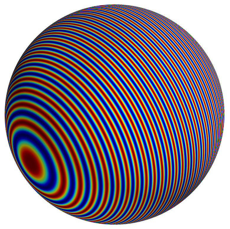
Figure 3: A sphere with $\kappa D=201.1$.

Table 1: Results of the sphere with the single-layer kernel.

$\varepsilon_{0}$	$\kappa D$	$N$	Time cost (sec)				Memory cost (MB)			$\varepsilon_{\text{a}}$
			$T_{\text{c}}$	$T_{\text{m}}$	$T_{\text{p}}$	$T_{\text{t}}$	$M_{\text{Q}}$	$M_{\text{m}}$	$M_{\text{t}}$
1e-3	12.6	4,608	1	5	$<$1	6	12	51	68	1.0e-3
1e-3	25.1	18,432	15	27	$<$1	43	125	294	518	2.7e-4
1e-3	50.3	73,728	129	103	2	236	1,013	1,406	2,671	4.4e-3
1e-3	100.5	294,912	812	429	11	1,265	6,414	6,083	14,011	5.5e-3
1e-3	201.1	1,143,072	4,054	1,866	79	6,053	31,987	26,241	62,579	8.8e-3
1e-6	12.6	4,608	5	44	$<$1	51	12	208	249	1.2e-6
1e-6	25.1	18,432	173	351	1	528	518	2,641	3,465	6.2e-6
1e-6	50.3	73,728	1,796	1,200	8	3,009	5,465	9,826	16,923	8.3e-6
1e-6	100.5	294,912	14,238	5,074	83	19,413	38,089	46,476	94,412	9.5e-6

Generally the overall error $\varepsilon_{\text{a}}$ is of the same magnitude with the predetermined parameter $\varepsilon$. The error $\varepsilon_{\text{a}}$ seems to grow with $\log N$. This is reasonable since in each level, some error of order $O(\varepsilon)$ is introduced, and there are $O(\log N)$ levels in the octree. Compared with the error of the dFMM in [2] from which our algorithm is transformed, the error becomes greater. This is because in our CBM, besides the low rank approximation of the kernel, extra error is introduced in the construction of curvelets with quasi-vanishing moments and the a-posteriori compression. Nevertheless, the overall error is still controllable.

In the $N$-body problem evaluations, most of the computational time are cost by construction of the explicitly-sparse representation of the system matrix, including the curvelet construction and matrix computation. Once the sparse representation is obtained, potentials on the target points can be evaluated very efficiently. A majority of the memory cost are taken by the storage of $\bm{Q}$ matrices and the sparse system matrix $\tilde{\bm{A}}_{\text{ns}}$, which are necessary for the curvelet transformation and matrix-vector multiplication in the curvelet space.

The time and memory cost by evaluations with $\varepsilon_{0}=$ 1e-3 are plotted in Figure 4 to show the computational complexity. It shows that the memory taken by storing $\tilde{\bm{A}}_{\text{ns}}$ is of order $O(N\log N)$, which means there are only log-linear nonzeros in the explicitly-sparse representation of the system matrix obtained by our algorithm. The time cost taken by the matrix computation also increases at the speed of $O(N\log N)$.

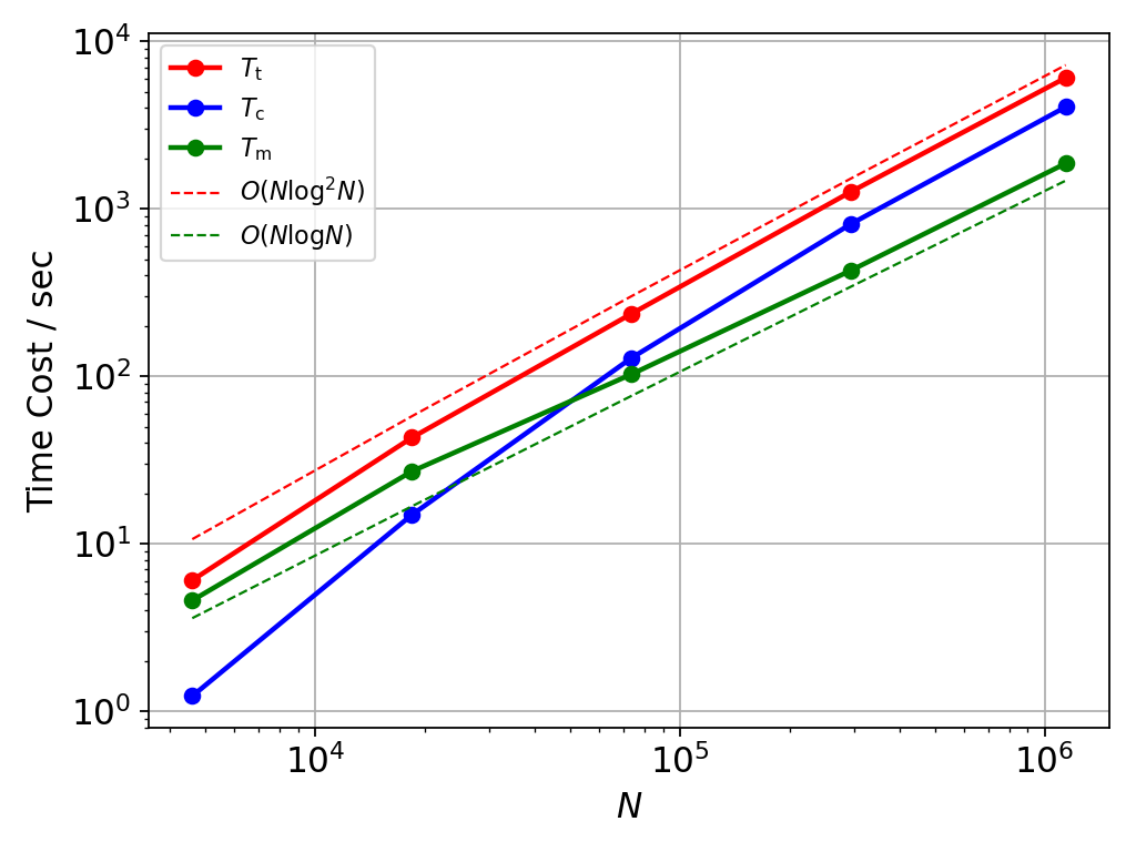
(a) Overall time cost.

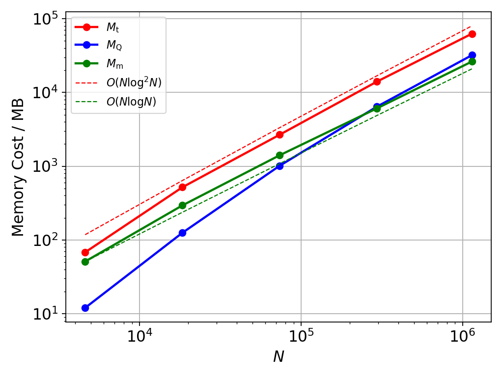
(b) Overall memory consumption.

Figure 4: Computational cost of the summation on a unit sphere with the single layer kernel.

Theoretically, the computational complexity of curvelet construction and the overall computation should also be $O(N\log N)$. For each level with the cube width being $w$, there are at most $O(D^{2}/w^{2})$ non-empty cubes since the points are sampled on a surface. And there are at most $O(\kappa^{2}w^{2})$ directional cones when the cube lies in the high frequency regime. The computational cost of curvelet construction for each directional cone is of order $O(1)$ since the dimension of the moment matrices and M2M matrices are independent of $\kappa w$. Therefore, the computational cost of curvelet construction in each level is of order $O(D^{2}/w^{2}\cdot\kappa^{2}w^{2})=O(\kappa^{2}D^{2})=O(N)$, and the overall computational complexity of curvelet construction in all levels should be $O(N\log N)$ since there are $O(\log N)$ levels in the octree.

However, it seems the time and memory cost in curvelet construction increases faster than the theoretical prediction, and the overall computational complexity seems $O(N\log^{2}N)$. To figure out the reason, we count the actual number of nonempty directional cones in the numerical cases. Notice that for a cube in the high frequency, if its interaction field in the directional cone is empty but there are nonempty cubes in the far field in this cone, the cone is still considered as nonempty, and curvelets and scaling functions have to be constructed since they are later required in the construction of its parent in higher levels. The number of nonempty cones differs from cube to cube, thus we compute its average value for each level. For each level with cube width in term of wavelength $w/\lambda=\kappa w/2\pi$, the average number of nonempty cones $\tilde{\Gamma}_{l}$ for each cone and its theoretical upper bound $\bar{\Gamma}_{l}$ are listed in Table 2.

Table 2: Number of nonempty directional cones in the $N$-body problem with points on a spherical surface.

$w/\lambda$	$\tilde{\Gamma}_{l}$				$\bar{\Gamma}_{l}$
	$\kappa D=8\pi$	$\kappa D=16\pi$	$\kappa D=32\pi$	$\kappa D=64\pi$
1	12.9	35.4	49.1	55.7	96
2	-	-	69.1	142.0	384

It is shown that in real-world numerical cases, the number of nonempty directional cones may be much less than the upper bound $\bar{\Gamma}_{l}\sim O(\kappa^{2}w^{2})$, and it tends to increase with frequency. This may be because the dimensionless curvature $\lambda/R$ of the surface on which the points locate reduces with the frequency. When the frequency is not so high, the curvature is relatively great, and the far-field surface tends to locate in a small number directional cones. But when the frequency gets higher, the curvature decreases and the surface tends to occupy more directional cones, as illustrated in Figure 5. Nevertheless, the number of directional cones will never exceed $\bar{\Gamma}_{l}\sim O(\kappa^{2}w^{2})$. Thus the computational complexity of curvelet construction should approach $O(N\log N)$ asymptotically as the frequency keep increasing. This trend has been partially demonstrated in Figure 4, in which the slope of $T_{\text{c}}$ reduces as the frequency increases. It is expected that the slope would further reduce to approximately parallel with that of $O(N\log N)$ if results of higher frequency cases are provided. However, they are not computed in this work due to the memory limit of our computer.

(a) Lower frequency, 6 nonempty cones.

(b) Higher frequency, 8 nonempty cones.

Figure 5: Increasement of the number of nonempty directional cones with frequency for the same $w/\lambda$. Illustrated with a two-dimensional case. Three-dimensional cases would be similar.

5.2 Kernels of other layers

The performance of our CBM with double, adjoint and quadrapole layers are studied in this section. The points are also sampled on the surface of a unit sphere, and their normals points outwards. The numerical results are listed in Table 3–5.

Table 3: Results of the sphere with the double-layer kernel.

$\varepsilon_{0}$	$\kappa D$	$N$	Time cost (sec)				Memory cost (MB)			$\varepsilon_{\text{a}}$
			$T_{\text{c}}$	$T_{\text{m}}$	$T_{\text{p}}$	$T_{\text{t}}$	$M_{\text{Q}}$	$M_{\text{m}}$	$M_{\text{t}}$
1e-3	12.6	4,608	1	5	$<$1	6	12	61	77	5.0e-4
1e-3	25.1	18,432	15	26	$<$1	43	125	388	559	1.1e-3
1e-3	50.3	73,728	124	95	2	225	1,013	1,901	3,177	1.2e-3
1e-3	100.5	294,912	786	403	35	1,238	6,465	8,515	16,518	1.7e-3
1e-3	201.1	1,143,072	4,065	1,738	83	5,941	32,884	38,000	74,970	1.8e-3
1e-6	12.6	4,608	6	48	$<$1	55	6	316	351	5.8e-7
1e-6	25.1	18,432	164	358	1	532	531	2,971	3,807	1.4e-6
1e-6	50.3	73,728	1,869	1,241	9	3,124	5,854	12,161	19,753	1.5e-6
1e-6	100.5	294,912	15,357	5,252	80	20,708	40,368	56,058	106,432	1.7e-6

Table 4: Results of the sphere with the adjoint-layer kernel.

$\varepsilon_{0}$	$\kappa D$	$N$	Time cost (sec)				Memory cost (MB)			$\varepsilon_{\text{a}}$
			$T_{\text{c}}$	$T_{\text{m}}$	$T_{\text{p}}$	$T_{\text{t}}$	$M_{\text{Q}}$	$M_{\text{m}}$	$M_{\text{t}}$
1e-3	12.6	4,608	1	5	$<$1	6	12	60	77	5.0e-4
1e-3	25.1	18,432	15	26	$<$1	41	125	388	559	1.1e-3
1e-3	50.3	73,728	127	96	2	228	1,012	1,901	3,177	1.2e-3
1e-3	100.5	294,912	786	403	34	1,237	6,465	8,515	16,518	1.7e-3
1e-3	201.1	1,143,072	4,068	1,732	82	5,937	32,884	38,000	74,970	1.8e-3
1e-6	12.6	4,608	5	44	$<$1	51	6	316	351	5.8e-7
1e-6	25.1	18,432	160	352	1	515	531	2,971	3,807	1.4e-6
1e-6	50.3	73,728	1,875	1,234	10	3,124	5,854	12,161	19,753	1.5e-6
1e-6	100.5	294,912	15,494	5,254	80	20,847	40,368	56,058	106,432	1.7e-6

Table 5: Results of the sphere with the quadrapole-layer kernel.

$\varepsilon_{0}$	$\kappa D$	$N$	Time cost (sec)				Memory cost (MB)			$\varepsilon_{\text{a}}$
			$T_{\text{c}}$	$T_{\text{m}}$	$T_{\text{p}}$	$T_{\text{t}}$	$M_{\text{Q}}$	$M_{\text{m}}$	$M_{\text{t}}$
1e-3	12.6	4,608	1	5	$<$1	6	12	46	62	8.0e-4
1e-3	25.1	18,432	14	25	$<$1	41	125	159	456	2.2e-4
1e-3	50.3	73,728	120	94	2	219	1,023	722	2,382	3.7e-3
1e-3	100.5	294,912	773	394	10	1,192	6,380	3,562	12,533	4.5e-3
1e-3	201.1	1,143,072	3,961	1,712	79	5,808	33,159	17,018	58,595	5.7e-3
1e-6	12.6	4,608	6	47	$<$1	54	0	324	353	4.0e-7
1e-6	25.1	18,432	164	352	1	519	546	2,347	3,196	6.4e-6
1e-6	50.3	73,728	1,943	1,241	9	3,196	6,216	8,624	16,677	6.5e-6
1e-6	100.5	294,912	17,068	5,340	77	22,502	43,356	39,995	94,160	1.2e-5

It is shown that the performance for the adjoint layer kernel is approximately the same with that for the double layer. This is reasonable since their matrices are in fact the transpose of each other, i.e., $\bm{A}^{\text{(a)}}=\overline{\bm{A}^{\text{(d)}}}$, where the superscript (a) and (d) represents the adjoint and double layer kernel, respectively. Since in our CBM we get the sparse representation $\bm{A}=\overline{\bm{Q}_{w}}\tilde{\bm{A}}_{\text{ns}}\bm{Q}_{\chi}$, thus theoretically, $\bm{Q}_{w}^{\text{(a)}}=\bm{Q}_{\chi}^{\text{(d)}},\tilde{\bm{A}}_{\text{ns}}^{\text{(a)}}=\overline{\tilde{\bm{A}}_{\text{ns}}^{\text{(d)}}}$, and $\bm{Q}_{\chi}^{\text{(a)}}=\bm{Q}_{w}^{\text{(d)}}$. Hence the computations for the adjoint layer kernel are the same with that for the double layer kernel, except that the position of target and source points are exchanged in the algorithm. The slight differences in the computational cost may come from the random choice of equivalent points in construction of low rank approximation for the kernel in high frequency regimes [28, 49].

The memory cost $M_{\text{m}}$ by storing $\tilde{A}_{\text{ns}}$ for the quadrapole layer is much less than that for the single layer. This is because, for the quadrapole layer kernel

$$\frac{\partial^{2}G(\bm{x},\bm{y})}{\partial\bm{n_{x}}\partial\bm{n_{y}}}=\left[(k^{2}r^{2}+3ikr-3)(\bm{\hat{r}}\cdot\bm{\hat{n}_{x}})(\bm{\hat{r}}\cdot\bm{\hat{n}_{y}})+(1-ikr)(\bm{\hat{n}_{x}}\cdot\bm{\hat{n}_{y}})\right]\frac{\text{e}^{ikr}}{4\pi r^{3}},$$ (40)

its hypersingularity makes it increases sharply when $\bm{x}$ approaches $\bm{y}$. Thus the elements in the near field can be much greater than that in the case with the single layer kernel. The norm of the transformed matrix block $\bm{A}^{\phi,\phi}$, and the threshold for the a-posteriori compression (37) would also become larger. Consequently, more tiny elements could be discarded in the a-posteriori compression, leaving less nonzero elements in the final explicitly-sparse representation, and less memory is consumed. The overall error $\varepsilon_{\text{a}}$ becomes greater but is still approximately of the same order with $\varepsilon$.

The memory cost $M_{\text{m}}$ for the double and adjoint layer, however, is greater than that for the single layer. This is because, for the double layer kernel

$$\frac{\partial G(\bm{x},\bm{y})}{\partial\bm{n_{y}}}=(1-ikr)\cdot(\bm{\hat{r}}\cdot\bm{\hat{n}_{y}})\frac{\text{e}^{ikr}}{4\pi r^{2}}$$ (41)

and the adjoint kernel

$$\frac{\partial G(\bm{x},\bm{y})}{\partial\bm{n_{x}}}=-(1-ikr)\cdot(\bm{\hat{r}}\cdot\bm{\hat{n}_{x}})\frac{\text{e}^{ikr}}{4\pi r^{2}},$$ (42)

the $\bm{\hat{r}}\cdot\bm{\hat{n}}$ term makes them approaches 0 when $\bm{x}$ approaches $\bm{y}$ since $\bm{x}$ and $\bm{y}$ are sampled on the surface with $\bm{n}$ is the surface normal. This makes the elements in the near field becomes much smaller than that in the case with the single layer kernel, and results in a smaller threhold for the a-posteriori compression. Consequently, more nonzero elements are left in the explicitly-sparse representation and more memory is consumed. The overall error $\varepsilon_{\text{a}}$ becomes lower probably because less error is introduced in the a-posteriori compression.

5.3 Different geometries

An aircraft X45X and a submarine DARPA suboff is used to study the performance of our CBM on different geometries. The CAD models are downloaded from grabcab.com. Various frequencies and different choices of $\varepsilon$ are considered. In the highest frequency case, the size of the aircraft is about 96 wavelengths, and the submarine is about 109 wavelengths long, as depicted in Figure 6 and 7. The points are also sampled with approximately 10 points per wavelength. The summations are computed with the single layer kernel. The computational results are listed in Table 6 and 7, in which the log-linear complexity is shown. Compared with summations on a sphere, higher frequency cases are computed for the aircraft and submarine within approximately the same computational cost, showing that our CBM is more efficient for flattened and elongated geometries. This is because with such geometries, more directional cones are empty, and less directional cones has to be addressed.

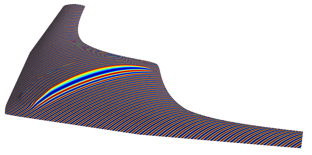
Figure 6: A aircraft with $\kappa D=603.2$.

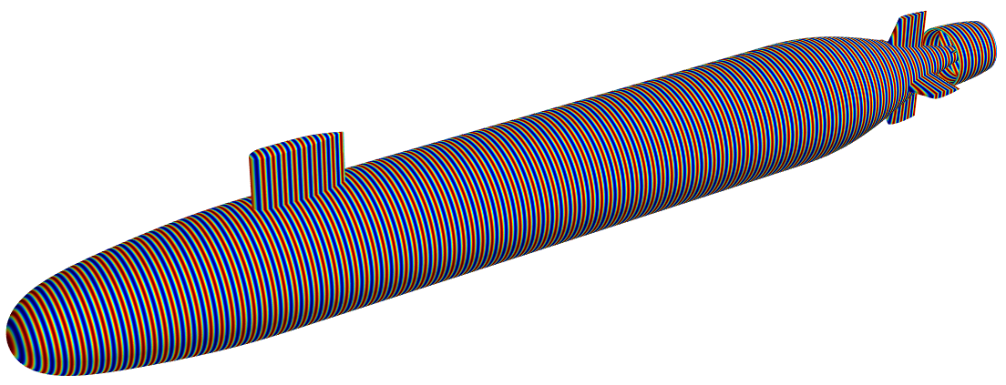
Figure 7: A submarine with $\kappa D=684.3$.

Table 6: Results of the aircraft with the single-layer kernel.

$\varepsilon_{0}$	$\kappa D$	$N$	Time cost (sec)				Memory cost (MB)			$\varepsilon_{\text{a}}$
			$T_{\text{c}}$	$T_{\text{m}}$	$T_{\text{p}}$	$T_{\text{t}}$	$M_{\text{Q}}$	$M_{\text{m}}$	$M_{\text{t}}$
1e-3	75.4	22,992	17	26	$<$1	45	155	308	565	2.0e-3
1e-3	150.8	88,608	114	107	2	226	1,026	1,738	3,024	1.4e-3
1e-3	301.6	350,388	763	501	25	1,305	6,547	8,180	16,121	1.7e-3
1e-3	603.2	1,401,348	3,920	2,035	99	6,139	35,612	34,059	74,600	1.7e-3
1e-6	75.4	22,992	149	283	2	438	614	2,557	3,454	9.5e-7
1e-6	150.8	88,608	1,091	1,370	9	2,481	4,708	13,770	20,157	8.9e-7
1e-6	301.6	350,388	6,570	5,910	82	12,603	30,559	64,361	102,260	1.2e-6

Table 7: Results of the submarine with the single-layer kernel.

$\varepsilon_{0}$	$\kappa D$	$N$	Time cost (sec)				Memory cost (MB)			$\varepsilon_{\text{a}}$
			$T_{\text{c}}$	$T_{\text{m}}$	$T_{\text{p}}$	$T_{\text{t}}$	$M_{\text{Q}}$	$M_{\text{m}}$	$M_{\text{t}}$
1e-3	85.5	21,348	12	25	$<$1	38	98	301	498	6.8e-4
1e-3	171.1	84,204	127	111	2	243	1,060	1,556	2,887	1.0e-3
1e-3	342.1	330,600	770	459	13	1,258	6,493	7,349	15,477	1.1e-3
1e-3	684.3	1,342,260	4,435	1,911	98	6,527	39,701	29,105	76,253	2.4e-3
1e-6	85.5	21,348	92	238	1	335	327	2,179	2,668	7.4e-7
1e-6	171.1	84,204	1,101	1,288	9	2,407	4,818	12,903	19,489	1.0e-6
1e-6	342.1	330,600	7,018	5,354	79	12,503	32,125	59,739	101,496	1.1e-6

6 Conclusion

A nearly optimal explicitly-sparse representation for oscillatory kernels is presented in this work by developing a curvelet based method. Here we summarize some of its main features:

• The explicitly-sparse representation of the system matrix only consists of $O(N\log N)$ nonzero elements.

• The computational complexity of the construction of the representation with controllable accuracy is log-linear.

• S2M, M2M, M2L, L2L, and L2T translation matrices in the directional FMM are used straightforwardly in our curvelet based method. As various techniques constructing the low rank approximation of the kernel can be used to compute the translation matrices, various variants of our curvelet based method can be easily developed.

• It is shown numerically that our method performs well for surface-distributed points with single, double, adjoint, and quadrapole layers, thus it is efficient for wave analysis with boundary integral equations as well.

Our curvelet based method is constructed as a transform of the directional FMM. It may also be viewed as the generalization of a wavelet based method to high frequency cases, and used as a new wideband fast algorithm. This work is expected to lay ground to future work related to new fast direct solvers and efficient preconditioners for high frequency problems.

References

- [1] Stephen Kirkup. The Boundary Element Method in Acoustics. Integrated Sound Software, 1998.
- [2] Yanchuang Cao, Lihua Wen, Jinyou Xiao, and Yijun Liu. A fast directional BEM for large-scale acoustic problems based on the Burton-Miller formulation. Engineering Analysis with Boundary Elements, 50:47–58, 2015.
- [3] Weng Cho Chew and Li Jun Jiang. Overview of large-scale computing: The past, the present, and the future. Proceedings of the IEEE, 101(2):227–241, 2013.
- [4] Zhaoneng Jiang, Xuguang Qiao, Wenfei Yin, Xiaoyan Zhao, Xiaofeng Xuan, and Ting Wan. A well-conditioned multilevel directional simply sparse method for analysis of electromagnetic problems. Engineering Analysis with Boundary Elements, 99:244–247, 2019.
- [5] Yanchuang Cao, Jinyou Xiao, Lihua Wen, and Zheng Wang. A fast directional boundary element method for wideband multi-domain elastodynamic analysis. Engineering Analysis with Boundary Elements, 108:210–216, 2019.
- [6] Stéphanie Chaillat and Marc Bonnet. Recent advances on the fast multipole accelerated boundary element method for 3D time-harmonic elastodynamics. Wave Motion, 50(7):1090–1104, 2013.
- [7] Yijun Liu. On the BEM for acoustic wave problems. Engineering Analysis with Boundary Elements, 107:53–62, 2019.
- [8] Fei Liu and Lexing Ying. Sparsify and sweep: an efficient preconditioner for the Lippmann-Schwinger equation. SIAM Journal on Scientific Computing, 40(2):B379–B404, 2018.
- [9] Björn Engquist and Lexing Ying. Sweeping preconditioner for the Helmholtz equation: Hierarchical matrix representation. Communications on Pure and Applied Mathematics, 64:697–735, 2011.
- [10] V. Rokhlin. Rapid solution of integral equations of classical potential theory. Journal of Computational Physics, 60:187–207, 1985.
- [11] L. Greengard and V. Rokhlin. A fast algorithm for particle simulations. Journal of Computational Physics, 73(2):325–348, 1987.
- [12] D. Zorin L. Ying, G. Biros. A kernel-independent adaptive fast multipole algorithm in two and three dimensions. Journal of Computational Physics, 196(2):591–626, 2004.
- [13] William Fong and Eric Darve. The black-box fast multipole method. Journal of Computational Physics, 228(23):8712–8725, 2009.
- [14] Josh Barnes and Piet Hut. A hierarchical force-calculation algorithm. Nature, 324:446–449, 1986.
- [15] W. Hackbusch and S. Börm. -matrix approximation of integral operators by inerpolation. Applied Numerical Mathematics, 43:129–143, 2002.
- [16] Mario Bebendorf. Approximation of boundary element matrices. Numer Math, 86(4):565–589, 2000.
- [17] M. Bebendorf and R. Venn. Constructing nested bases approximations from the entries of non-local operators. Numerische Mathematik, 121(4):609–635, 2012.
- [18] Vaishnavi Gujjula and Sivaram Ambikasaran. A new nested cross approximation. arXiv: 2203.14832, 2022.
- [19] C C Lu and W C Chew. Fast algorithm for solving hybrid integral equations. IEE Proc. H, 140:455–460, 1993.
- [20] V. Rokhlin. Diagonal forms of translation operators for the Helmholtz equation in three dimensions. Applied and Computational Harmonic Analysis, 1:82–93, 1993.
- [21] L. Greengard and V. Rokhlin. A new version of the fast multipole method for the Laplace equation in three dimensions. Acta Numerica, 6(1):229–269, 1997.
- [22] Eric Darve. The fast multipole method: Numerical implementation. Journal of Computational Physics, 160(1):195–240, 2000.
- [23] N Nishimura. Fast multipole accelerated boundary integral equation methods. Applied Mechanics Reviews, 55(4):299–324, 2002.
- [24] R Coifman, V Rokhlin, and S Wandzura. The fast multipole method for the wave equation: A pedestrian prescription. IEEE Antennas and Propagation Magazine, 35:7–12, 1993.
- [25] B Dembart and E Yip. The accuracy of fast multipole methods for Maxwell’s equations. IEEE Comput. Sci. Eng., 5(3):48–56, 1998.
- [26] Hongwei Cheng, William Y. Crutchfield, Zydrunas Gimbutas, Leslie F. Greengard, J. Frank Ethridge, Jingfang Huang, Vladimir Rokhlin, Norman Yarvin, and Junsheng Zhao. A wideband fast multipole method for the Helmholtz equation in three dimensions. Journal of Computational Physics, 216(1):300–325, 2006.
- [27] Nail A. Gumerov and Ramani Duraiswami. A broadband fast multipole accelerated boundary element method for the three dimensional Helmholtz equation. Journal of the Acoustical Society of America, 125(1):191–205, 2009.
- [28] Björn Engquist and Lexing Ying. Fast directional multilevel algorithms for oscillatory kernels. SIAM Journal on Scientific Computing, 29(4):1710–1737, 2007.
- [29] Matthias Messner, Martin Schanz, and Eric Darve. Fast directional multilevel summation for oscillatory kernels based on Chebyshev interpolation. Journal of Computational Physics, 231(4):1175–1196, 2012.
- [30] Austin R. Benson, Jack Poulson, Kenneth Tran, Björn Engquist, and Lexing Ying. A parallel directional fast multipole method. SIAM Journal of Scientific Computing, 36(4):C335–C352, 2014.
- [31] Mario Bebendorf, Christian Kuske, and Raoul Venn. Wideband nested cross approximation for Helmholtz problems. Numerische Mathematik, 130(1):1–34, 2015.
- [32] Vaishnavi Gujjula and Sivaram Ambikasaran. A new Directional Algebraic Fast Multipole Method based iterative solver for the Lippmann-Schwinger equation accelerated with HODLR preconditioner. Commun. Comput. Phys., 32:1061–1093, 2022.
- [33] Sivaram Ambikasaran and Eric Darve. The inverse fast multipole method. arXiv: 1407.1572v1, 2014.
- [34] Pieter Coulier, Hadi Pouransari, and Eric Darve. The inverse fast multipole method: Using a fast approximate direct solver as a preconditioner for dense linear systems. Computer Science, 39(3):A761–A796, 2017.
- [35] G. Beylkin, R. Coifman, and V. Rokhlin. Fast wavelet transforms and numerical algorithms I. Communications on Pure and Applied Mathematics, 44(2):141–183, 1991.
- [36] Johannes Tausch and Jacob White. Multiscale bases for the sparse representation of boundary integral operators on complex geometry. SIAM J. Sci. Comput., 24(5):1610–1629, 2003.
- [37] Johannes Tausch. A variable order wavelet method for the sparse representation of layer potentials in the non-standard form. Journal of Numerical Mathematics, 12(3):233–254, 2004.
- [38] Jinyou Xiao, Johannes Tausch, and Lihua Wen. Approximate moment matrix decomposition in wavelet Galerkin BEM. Computer Methods in Applied Mechanics and Engineering, 197:4000–4006, 2008.
- [39] Daan Huybrechs, Jo Simoens, and Stefan Vandewalle. A note on wave number dependence of wavelet matrix compression for integral equations with oscillatory kernel. Journal of Computational and Applied Mathematics, 172:233–246, 2004.
- [40] Stuart C. Hawkins, Ke Chen, and Paul J. Harris. On the influence of the wavenumber on compression in a wavelet boundary element method for the Helmholtz equation. International Journal of Numerical Analysis and Modeling, 4(1):48–62, 2007.
- [41] Jinyou Xiao, Lihua Wen, and Johannes Tausch. On fast matrix-vector multiplication in wavelet Galerkin BEM. Engineering Analysis with Boundary Elements, 33(2):159–167, 2009.
- [42] Jinyou Xiao and Johannes Tausch. A fast wavelet-multipole method for direct BEM. Engineering Analysis with Boundary Elements, 34:673–679, 2010.
- [43] Emmanuel J. Candès and David L. Donoho. Curvelets: A Surprisingly Effective Nonadaptive Representation for Objects with Edges, pages 105–120. Nashville: Vanderbilt University Press, 2000.
- [44] Emmanuel Candès, Laurent Demanet, David Donoho, and Lexing Ying. Fast discrete curvelet transforms. Multiscale Model. Simul., 5(3):861–899, 2006.
- [45] Jianwei Ma and Gerlind Plonka. The curvelet transform: A review of recent applications. IEEE Signal Processing Magazine, 27(2):118–133, 2010.
- [46] Emmanuel J. Candès and Laurent Demanet. The curvelet representation of wave propagators is optimally sparse. Communications on Pure and Applied Mathematics, 58:1472–1528, 2005.
- [47] Jinyou Xiao and Wenjing Ye. Wavelet BEM for large-scale Stokes flows based on the direct integral formulation. International Journal for Numerical Methods in Engineering, 88:693–714, 2011.
- [48] Jinyou Xiao, Johannes Tausch, and Yucai Hu. A-posteriori compression of wavelet-BEM matrices. Comput. Mech., 44:705–715, 2009.
- [49] Björn Engquist and Lexing Ying. Fast directional algorithms for the Helmholtz kernel. Journal of Computational and Applied Mathematics, 234(6):1851–1859, 2010.