Bulk Landau Pole and Unitarity of Dual Conformal Field Theory

Abstract

The singlet sector of the $O(N)$ $\phi^{4}$-model in AdS₄ at large-$N$, gives rise to a dual conformal field theory on the conformal boundary of AdS₄, which is a deformation of the generalized free field. We identify and compute an AdS₄ three-point one-loop fish diagram that controls the exact large-$N$ dimensions and operator product coefficients (OPE) for all “double trace” operators as a function of the renormalized $\phi^{4}$-couplings. We find that the space of $\phi^{4}$-coupling is compact with a boundary at the bulk Landau pole. The dual CFT is unitary only in an interval of negative couplings bounded by the Landau pole where the lowest OPE coefficient diverges.

1 Introduction

To characterize an interacting quantum field theory in Minkowski space-time we need to know the masses and spins of its asymptotic states as well as the $S$-matrix elements between them. In curved space-time there is no notion of $S$-matrix but in maximally symmetric spaces such as de Sitter (dS₄) or anti-de Sitter (AdS₄) space-time correlation functions evaluated on their conformal boundary define a conformal field theory (CFT). Therefore, an interacting quantum field theory in these spaces is characterized completely in terms of the conformal dimensions of the primary fields of that CFT and their operator product expansion coefficients (OPE). This program has been outlined in Heemskerk et al. (2009) and further explored in many subsequent works, including Fitzpatrick and Kaplan (2012); Penedones (2011).

In this note we consider a conformally coupled scalar field theory with $\phi^{4}$ interaction in four-dimensional AdS. A free scalar in AdS₄ with Dirichlet boundary conditions on its conformal boundary, is encoded in the CFT of a generalized free field Heemskerk et al. (2009) of conformal dimension $2$. The OPEs of the latter have been determined in Heemskerk et al. (2009); Fitzpatrick and Kaplan (2012) by comparing the four-point correlation function Mueck and Viswanathan (1998) with the conformal block expansion Dolan and Osborn (2001). They give rise to double trace operators, in terminology analogous to four-dimensional Yang-Mills theory, which is holographically dual to string theory in AdS${}_{5}\times S^{5}$. Bulk quantum field theories in AdS₅, being non-renormalizeable, are usually defined as being “the dual” of a given boundary CFT. The present approach is the opposite: we construct a three-dimensional boundary CFT for a given renormalizeable bulk field theory in four-dimensional AdS. The $\phi^{4}$ interaction does not affect the spectrum of the CFT in perturbation theory, but the dimensions and OPE coefficients of double trace operators are corrected Heemskerk et al. (2009); Fitzpatrick and Kaplan (2012). The one-loop correction to the bulk correlations function and thereby the CFT data was then found in Bertan et al. (2019); Bertan and Sachs (2018); Heckelbacher et al. (2022). The calculation of the loop integrals as well as the conformal block expansion at this order is rather exhaustive, but an extension to higher loops is not an easy task (see Heckelbacher et al. (2022) for a discussion). On the other hand it is well-known that in Minkowski space an all loop extension is available in the large-$N$ limit of the ${\lambda\over N}(\phi_{i}\phi^{i})^{2}$ theory or $O(N)$ model (e.g. Moshe and Zinn-Justin (2003) for a review). The leading large-$N$ contribution of the four-point function is given by the sum of a necklace of multi-bubble diagrams which, thanks to momentum conservation, are just the power of the one-loop bubble. In the large-$N$ limit the perturbative corrections can be summed into

$$W(p)\sim\lambda\frac{\delta^{(4)}(p_{1}+\dots+p_{4})}{1-B(|p_{1}+p_{2}|)},$$ (1)

where $B(p)$ is the one-loop four-point bubble contribution. However, it was shown in Coleman et al. (1974) that this features a tachyonic mode in large-$N$ limit. We identify a manifestation of that pathology in AdS₄. This requires a resummation of the multi-loop bubble diagrams in AdS₄ which has so far been elusive. Here we solve this problem and derive the associated renormalized spectral function $\mathcal{B}_{\rm ren}(\nu)$ in eq. (27).

2 Tree-Level Diagrams

Quite generally, the relation of AdS₄ boundary four-point functions $W(\vec{x}_{i})$, to correlators of a three-dimensional CFT primary field $\mathcal{O}_{2}(\vec{x})$ of dimension 2 is given by

$$\langle\mathcal{O}_{2}(\vec{x}_{1})\cdots\mathcal{O}_{2}(\vec{x}_{4})\rangle =W(\vec{x}_{1},\vec{x}_{2},\vec{x}_{3},\vec{x}_{4})$$ (2)

We consider the Poincaré patch with coordinates $X=\{\vec{x},z\}\in\mathbb{R}^{3}\times\mathbb{R}_{+}$. The CFT four-point function has an expansion in terms of conformal blocks as

$$W(\vec{x}_{1},\vec{x}_{2},\vec{x}_{3},\vec{x}_{4})=\int_{\mathbb{R}}\frac{\differential\nu}{2\pi}D(\nu)g(\vec{x}_{1},\vec{x}_{2},\vec{x}_{3},\vec{x}_{4};\nu)$$ (3)

where

$$g(\vec{x}_{i};\nu)\propto\int\limits_{\partial AdS_{4}}\differential^{3}\vec{x}\langle\mathcal{O}_{2}(\vec{x}_{1})\mathcal{O}_{2}(\vec{x}_{2})\mathcal{O}_{\nu}(\vec{x})\rangle\langle\tilde{\mathcal{O}}_{-\nu}(\vec{x}){\mathcal{O}}_{2}(\vec{x}_{3}){\mathcal{O}}_{2}(\vec{x}_{4})\rangle$$ (4)

encodes the contribution of an internal double trace operator $\mathcal{O}_{\nu}(\vec{x})$ (and its descendants) of conformal dimension $\Delta(\nu)=\frac{3}{2}+i\nu$, and $\tilde{\mathcal{O}}_{-\nu}$ is the “shadow” primary field of dimension $3-$dim$[\mathcal{O}_{\nu}]=3/2-i\nu$ (see for instance (Meltzer et al., 2020, §2)). The dimension of the internal primaries are then given by the poles of the spectral function $D(\nu)$ while the OPE coefficients into the double trace operators are encoded in the residues of the latter. Conversely, $D(\nu)$ is obtained by integrating $W(\vec{x}_{i})$ against a CFT three-point function

$$\langle\mathcal{O}_{\Delta}(\vec{x}_{1})\mathcal{O}_{\Delta}(\vec{x}_{2})\mathcal{O}_{\nu}(\vec{x}_{0})\rangle=\frac{1}{x_{12}^{2\Delta-\Delta(\nu)}x_{10}^{\Delta(\nu)}x_{20}^{\Delta(\nu)}}$$ (5)

which satisfies an orthogonality relation

$$\int\limits_{\partial\text{AdS}_{4}}\differential^{3}x_{1}\differential^{3}x_{2}\langle\mathcal{O}_{\nu}(\vec{x})\mathcal{O}_{2}(\vec{x}_{1})\mathcal{O}_{2}(\vec{x}_{2})\rangle\langle\tilde{\mathcal{O}}_{1}(\vec{x}_{1})\tilde{\mathcal{O}}_{1}(\vec{x}_{2})\mathcal{O}_{-\nu^{\prime}}(\vec{x}^{\prime})\rangle\cr=\frac{4\pi^{4}|\Gamma(i\nu)|^{2}}{|\Gamma(\frac{3}{2}+i\nu)|^{2}}\delta(\nu-\nu^{\prime})\delta(\vec{x}-\vec{x}^{\prime})\,.$$ (6)

Disconnected four-point function: Dismissing the identity conformal block we have

$$W^{(\textrm{disc})}(\vec{x}_{1},\vec{x}_{2},\vec{x}_{3},\vec{x}_{4})=\frac{1}{(x^{2}_{13}x^{2}_{24})^{2}}+\frac{1}{(x^{2}_{14}x^{2}_{23})^{2}}\,.$$ (7)

The result for the spectral function was given in Heemskerk et al. (2009); Fitzpatrick and Kaplan (2012)

$$D^{(\textrm{disc})}(\nu)=\frac{2\pi^{\frac{3}{2}}|\Gamma(\frac{5}{4}+i\frac{\nu}{2})|^{2}\Gamma(\frac{3}{2}-i\nu)\Gamma(\frac{3}{4}+i\frac{\nu}{2})^{2}}{|\Gamma(\frac{1}{4}+i\frac{\nu}{2})|^{2}\Gamma(i\nu)\Gamma(\frac{3}{4}-i\frac{\nu}{2})^{2}}\,,$$ (8)

whose simple poles and their residues imply the (mean field) double trace dimensions and OPE’s as in Heemskerk et al. (2009)

$$\nu_{n}=-i\left(\frac{5}{2}+2n\right)\;;\qquad|\bar{c}(\nu_{n})|^{2}=i\text{Res}D^{(\textrm{disc})}(\nu_{n})\,.$$ (9)

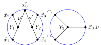
Figure 1: Sketch of the integration of the bulk four-point function left (with resolved $\delta$-function vertex as in (10)) against the three-point function with two shadow operators $\langle\tilde{\mathcal{O}}_{1}(\vec{x}_{3})\tilde{\mathcal{O}}_{1}(\vec{x}_{4})\mathcal{O}_{-\nu}(\vec{x})\rangle$ on the right to extract $D(\nu)$.

Cross diagram: Here we evaluate the spectral function using a different method that will be useful at loop level. As represented in the diagram on the left of fig. 1, we resolve the bulk four-point vertex using the representation of the delta-function Meltzer et al. (2020)

$$\delta(Y_{1}-Y_{2})=\int\limits_{-\infty}^{\infty}\frac{\differential\nu\nu^{2}}{\pi}\int\limits_{\partial\text{AdS}_{4}}\differential^{3}x\bar{\Lambda}_{\Delta(\nu)}(\vec{x},Y_{1})\bar{\Lambda}_{\Delta(-\nu)}(\vec{x},Y_{2})$$ (10)

in terms of the bulk-to-boundary propagator

$$\bar{\Lambda}_{\Delta}(\vec{x},X^{\prime})=\frac{n_{\Delta}z^{\prime\Delta}}{\left((\vec{x}^{\prime}-\vec{x})^{2}+z^{\prime 2}\right)^{\Delta}}\,,\qquad{n_{\Delta}}=\frac{\Gamma\left(\Delta\right)}{2\pi^{\frac{3}{2}}\Gamma(\Delta-\frac{1}{2})}.$$ (11)

for a scalar of mass $m^{2}=-\frac{9}{4}-\nu^{2}$ and dimension $\Delta(\nu)=\frac{3}{2}+i\nu$. In conjunction with (3)-(4) this shows that the tree-level spectral function for the cross diagram $D^{(\times)}(\nu)$ is given by (the coupling constant $\lambda$ times) the relative normalizations of the CFT three-point correlator entering in (6) and the bulk three-point function

$$W_{\nu}^{(0)}(\vec{x}_{1},\vec{x}_{2},\vec{x}_{0}) =\int\limits_{\textrm{AdS}_{4}}\differential Y\bar{\Lambda}_{2}(\vec{x}_{1},Y)\bar{\Lambda}_{2}(\vec{x}_{2},Y)\bar{\Lambda}_{\Delta(\nu)}(\vec{x}_{0},Y)$$ (12)

$$={|\Gamma(\frac{5}{4}+i\frac{\nu}{2})|^{2}\Gamma(\frac{3}{4}+i\frac{\nu}{2})^{2}\over 4\pi^{4}\Gamma(1+i\nu)}{1\over x_{12}^{4-\Delta(\nu)}x_{10}^{\Delta(\nu)}x_{20}^{\Delta(\nu)}}\,.$$ (13)

Therefore

$$D^{(\times)}(\nu)=-\frac{\lambda}{2\pi^{5/2}}\frac{|\Gamma(\frac{5}{4}+i\frac{\nu}{2})|^{4}\Gamma(\frac{3}{4}+i\frac{\nu}{2})^{4}}{\Gamma(i\nu)\Gamma(\frac{3}{2}+i\nu)}\,,$$ (14)

which now has double poles. Comparing this with the perturbative series of the conformal block expansion (3)

$$W(\vec{x}_{1},\dots,\vec{x_{4}})=\sum\limits_{n}|\bar{c}_{\nu(n)}|^{2}g(\vec{x}_{i};\nu_{n})-i\sum\limits_{n}|\bar{c}_{\nu(n)}|^{2}\gamma^{(1)}_{n}\partial_{\nu}g(\vec{x}_{i};\nu)|_{\nu_{n}}\cr+\sum\limits_{n}(|\bar{c}|^{2}_{\nu(n)})^{(1)}\gamma^{(1)}_{n}g(\vec{x}_{i};\nu_{n})\,,$$ (15)

one then identifies the first order double trace anomalous dimensions $\gamma^{(1)}_{n}$ and squared OPE’s $(|c(\nu_{n})|^{2})^{(1)}$ as

$$\gamma^{(1)}_{n}=i\frac{\text{Res}D^{(\times)}(\nu_{n})}{\text{Res}D^{(\textrm{disc})}(\nu_{n})}=\frac{\lambda}{16\pi^{2}}$$ (16)

and

$$(|c(\nu_{n})|^{2})^{(1)}=\frac{\partial\text{Res}D^{(\textrm{disc})}(\nu_{n})}{\partial{\nu_{n}}}=\frac{1}{2}\frac{\partial|\bar{c}(\nu_{n})|^{2}}{\partial{n}}\,,$$ (17)

thus reproducing the expression given in Fitzpatrick and Kaplan (2012).

Figure 2: $s$-channel one-loop bubble

3 One-loop Diagram

A key observation for determining the spectral function directly for the one-loop amplitude in fig. 2 is to use the delta-function (10) to factorize the correlator into three-point functions as in fig. 3 and use the orthogonality relation (6) to express the one-loop graph spectral function in term of the fish three-point function $W^{(\rangle\!\bigcirc\!-)}_{\nu}(\vec{x}_{1},\vec{x}_{2},\vec{x}_{0})$ of fig. 4

$$D^{(\rangle\!\bigcirc\!\langle)}(\nu)=D^{(\times)}(\nu)\times\frac{W^{(\rangle\!\bigcirc\!-)}_{\nu}(\vec{x}_{1},\vec{x}_{2},\vec{x}_{0})}{W^{(0)}_{\nu}(\vec{x}_{1},\vec{x}_{2},\vec{x}_{0})}.$$ (18)

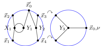
Figure 3: Sketch of the reduction of the one-loop bubble in fig. 2 to the fish diagram of fig. 4.

Figure 4: Three point fish diagram

The fish diagram has the ultraviolet divergence for colliding bulk points familiar from flat space which we regulate using the AdS-invariant cut-off introduced in Bertan et al. (2019). This amounts to modify the bulk-to-bulk propagator as

$$\Lambda^{\delta}(X,X^{\prime})={4z^{2}z^{\prime 2}\over(1+\delta)^{2}((\vec{x}-\vec{x}^{\prime})^{2}+z^{2}+z^{\prime 2})^{2}-4z^{2}z^{\prime 2}}$$ (19)

so that it is finite for coincident bulk points, $\Lambda^{\delta}(X,X)={1\over\delta(\delta+2)}$, $\delta>0$. The $X_{1}$ integral then proceeds as in (Heckelbacher et al., 2022, §4.2.2) to give

$$W_{\nu}^{(\rangle\!\bigcirc\!-)}(\vec{x}_{1},\vec{x}_{2},\vec{x}_{0})= \frac{-\lambda^{2}}{32\pi^{2}}\frac{n_{\Delta}^{2}n_{\Delta(\nu)}}{x_{10}^{\Delta(\nu)}x_{20}^{\Delta(\nu)}x_{12}^{4-\Delta(\nu)}}$$ (20)

$$\times\int\limits_{\mathbb{R}_{+}^{4}}{\differential^{4}Xz^{\Delta(\nu)}\over|X|^{4}|X-\vec{w}_{2}|^{4}}\left(\log 2\delta+2+\log\left(\frac{z^{2}|\vec{w}_{2}|^{2}}{|X|^{2}|\vec{w}_{2}-X|^{2}}\right)\right).$$

where $\vec{w}_{2}=\vec{x}_{2}/|\vec{x}_{2}|$. It is then clear from rotation invariance that the integral can only depend on $\nu$. Furthermore, the ultraviolet divergence from the collapsing loop in fig. 4 is proportional the three point function (12). The renomalization scheme of Bertan et al. (2019); Heckelbacher et al. (2022) amounts to subtracting from $W_{\nu}^{(\rangle\!\bigcirc\!-)}(\vec{x}_{i})$ the counter-term $\frac{\lambda^{2}}{32\pi^{2}}(\log(\delta/2)+\frac{11}{3})\,W_{\nu}^{(0)}(\vec{x}_{i})$. The logarithmic term in the integrand is conveniently written as a $\nu$-derivative. Then, making use of (12) we can read off the renormalised one-loop spectral function

$$D_{\rm ren}^{(\rangle\!\bigcirc\!\langle)}(\nu)=\frac{\lambda_{R}}{32\pi^{2}}\Big{(}\log(4)-\frac{5}{3}+\psi\left(\frac{5}{4}+i\frac{\nu}{2}\right)+\psi\left(\frac{5}{4}-i\frac{\nu}{2}\right)-2\psi(2)\Big{)}D^{(\times)}(\nu)\,,$$ (21)

where $\psi(x)=\Gamma^{\prime}(x)/\Gamma(x)$ is the digamma function and the renomalized coupling constant satisfies

$$\frac{16\pi^{2}}{\lambda}=\frac{16\pi^{2}}{\lambda_{R}}+\frac{1}{2}\left(\log(\frac{\delta}{2})+\frac{11}{3}\right)\,.$$ (22)

The function (21), together with $D^{(\times)}(\nu)$ provides closed expressions for all one-loop $s$-channel anomalous dimensions and OPE’s, which can be checked to agree numerically with the ones previously obtained in Bertan and Sachs (2018); Heckelbacher et al. (2022). Note that (21) is structurally similar to the spectral function obtained previously in Carmi (2020) for AdS₂ and AdS₃, ingeniously using the bootstrap approach. However, we will see that the physics derived form (21) is rather different.

4 Large-$N$ $O(N)$ Model

We now consider the curved space version of the vector model where the scalar field $\phi$ transforms in the fundamental representation of $O(N)$, together with the ${\lambda\over 4N}(\phi_{i}\phi^{i})^{2}$ interaction. We will focus on the CFT data encoding the singlet sector. Thus, we consider the large-$N$ limit of the conformal block expansion of the singlet four-point function

$${1\over N^{2}}\langle\mathcal{O}_{i}(\vec{x}_{1})\mathcal{O}^{i}(\vec{x}_{2})\mathcal{O}_{p}(\vec{x}_{3})\mathcal{O}^{p}(\vec{x}_{4})\rangle=\int\limits_{\mathbb{R}}{\differential\nu\over 2\pi}D(\nu)c_{ii}c_{pp}g(\vec{x}_{1},\dots,\vec{x}_{4},\nu)+O(1/N^{2}).$$ (23)

The identity OPE is $O(1)$ in the large-$N$ limit, while the disconnected contribution to the double trace dimension $\Delta$ and (squared) OPE’s $|\bar{c}|^{2}$ is again given by (8) after re-scaling by $1/N$. For the cross diagram with interaction vertex

$$\frac{\lambda}{N}\left(\delta_{ij}\delta_{pq}+\delta_{ip}\delta_{jq}+\delta_{iq}\delta_{jp}\right)\,,$$ (24)

the first term in the bracket dominates, at large $N$, for the singlet correlator (23). This then results in (16) and (17) for the anomalous dimension and OPE, after re-scaling $\text{Res}D^{(\textrm{disc})}$ and $\text{Res}D^{(\times)}$ both with $1/N$. At one-loop and large-$N$ the $s$-channel in fig. 2 dominates and by consequence the $D^{(\rangle\!\bigcirc\!\langle)}_{\rm ren}(\nu)$ is again given by (21) rescaled by $1/N$.

To see the resummation of the $s$-channel bubble diagrams we first give an alternative representation of the bubble diagram in fig. 2 as a product of two cross diagrams, using the split representation  Costa et al. (2014) depicted in fig. 5. However, we need to modify this representation to treat the aforementioned ultraviolet divergence for coincident bulk points. The regularized bulk-to-bulk propagator has the split representation

$$\Lambda^{\delta}(X_{1},X_{2})=\int\limits_{-\infty}^{+\infty}{\nu^{2}d\nu\over\pi}\int\limits_{\partial AdS_{4}}{\differential^{3}x\bar{\Lambda}_{\nu}(\vec{x},X_{1})\bar{\Lambda}_{-\nu}(\vec{x},X_{2})\over\nu^{2}+\frac{1}{4}+f(\nu,\delta)},$$ (25)

where $f(\nu,\delta)$ can be chosen in such a way as to reproduce the $\delta$-regularization introduced in (19). The ultraviolet divergences arise from the large-$\nu$ behaviour are then regulated by the $\delta$ regularisation. The precise choice of regulation is not important here as long as it preserves AdS-invariance. For instance, a cut-off regulator on the integral or zeta-function regularisation as in Giombi et al. (2013) could also be used.

Figure 5: The split representation of $W^{(\rangle\!\bigcirc\!\langle)}(\vec{x}_{1},\dots,\vec{x}_{4})$ in fig. 2 as a product of two cross diagrams.

After adding the counter term restoring the factor $\frac{\lambda_{R}^{2}}{2}$, the one-loop diagram in fig. 2 then takes the form

$$W_{\rm ren}^{(\rangle\!\bigcirc\!\langle)}(\vec{x}_{i})=\frac{\lambda_{R}}{2}\int_{\mathbb{R}}\differential\nu D^{(\times)}(\nu)\mathcal{B}_{\rm ren}(\nu)g(\vec{x}_{i};\nu).$$ (26)

For convenience we expressed the one-loop spectral function (21) as the product of $D^{(\times)}(\nu)$ and the one-loop bubble function

$$\mathcal{B}_{\rm ren}(\nu)=\frac{\lambda_{R}}{32\pi^{2}}\Big{(}\log(4)-\frac{5}{3}+\psi\left(\frac{5}{4}+i\frac{\nu}{2}\right)+\psi\left(\frac{5}{4}-i\frac{\nu}{2}\right)-2\psi(2)\Big{)}\,.$$ (27)

The advantage of the split representation is that it straight forwardly extends to the two-loop diagram. It is not hard to see that the two-loop necklace contribution $W^{(2)}(\vec{x}_{1},\dots,\vec{x}_{4})$ from (26) by replacing $\mathcal{B}_{\rm ren}(\nu)$ by $(\mathcal{B}_{\rm ren}(\nu))^{2}$. In this way, the multi-bubble diagrams can be summed up resulting in

$$W_{\rm ren}(\vec{x}_{1},\dots,\vec{x}_{4}) :=\sum\limits_{k=1}^{\infty}W^{(k)}_{\rm ren}(\vec{x}_{1},\dots,\vec{x}_{4})$$ (28)

$$=\int\limits_{-\infty}^{+\infty}\frac{\differential\nu}{2\pi}\frac{D^{(\times)}(\nu)}{1-{\mathcal{B}}_{\rm ren}(\nu)}g(\vec{x}_{1},\dots,\vec{x}_{4};\nu).$$

In the flat space limit $\nu\propto|p|\to\infty$ where $p$ is the four dimensional momentum, $\mathcal{B}_{\rm ren}(\nu)$ in the integrand of (28) gives the generalization of flat space expression in (1). This will be discussed further below when comparing with the flat space results of Coleman et al. (1974). The disadvantage of the split representation is however that a closed expression form of $\mathcal{B}_{\rm ren}(\nu)$ in the Mellin representation is not available. Luckily we don’t need it since we already evaluated $\mathcal{B}_{\rm ren}(\nu)$ in a different way in (21).

Thanks to the fall-off of the conformal block Ponomarev (2020), the contour can be closed in the lower half $\nu$-plane. There are two types of poles that contribute to the integral (28): i) The double poles of $D^{(\times)}(\nu)$ in eq. (14) and ii) The zeroes of $1-\mathcal{B}_{\rm ren}(\nu)$. The set i) coincides with the poles $\nu_{n}$ of $\mathcal{B}_{\rm ren}(\nu)$, so that, using (16), the integral has just simple poles of $O(\lambda_{R}^{0})$. Furthermore,

$$\stackrel{{\scriptstyle[}}{{\nu}}=\nu_{n}]{}{\textrm{Res}}\left(\frac{iD^{(\times)}(\nu)}{1-{\mathcal{B}}_{\rm ren}(\nu)}\right)={1\over\gamma^{(1)}}\stackrel{{\scriptstyle[}}{{\nu}}=\nu_{n}]{}{\textrm{Res}}((\nu-\nu_{n})D^{(\times)}(\nu))=-|\bar{c}(\nu_{n})|^{2}$$ (29)

and thus does cancel the disconnected (mean field) contribution. This is required by consistency since otherwise the mean field double trace operators would continue to contribute at finite coupling $\lambda$. Concerning ii) we need to solve the equation $\mathcal{B}_{\rm ren}(\nu)=1$ or, equivalently (see also Carmi et al. (2019); Carmi (2020))

$$\log(4)-\frac{5}{3}+\psi\left(\frac{5}{4}+i\frac{\nu}{2}\right)+\psi\left(\frac{5}{4}-i\frac{\nu}{2}\right)-2\psi(2)=\frac{32\pi^{2}}{\lambda_{R}}\,.$$ (30)

For $\lambda_{R}=0$ the solutions of (30) are given by the poles of $\psi\left(\frac{5}{4}+i\frac{\nu}{2}\right)$ which correspond the double trace dimensions in the mean field theory. Then, increasing $\lambda_{R}$, the double trace dimensions grow in accordance with perturbation theory approaching a finite value at for $\frac{1}{\lambda_{R}}\to 0_{+}$. This function can then be continuously be extended to negative values of $\frac{1}{\lambda_{R}}$ down to the critical coupling

$${32\pi^{2}\over\lambda_{*}}=\frac{13}{3}-4\ln\!\left(2\right)-\pi\simeq-1.58$$ (31)

where eq. (30) is solved for $\nu=0$. At this point a new double trace operator of dimensions $\Delta(0)={3\over 2}$ appears. All this is represented in fig. 6. For $\lambda_{*}\leq\lambda_{R}\leq 0$ this solution $\nu_{0}$ (in green) moves down the negative imaginary axis with the dimensions of the first double trace operator covering the interval ${3\over 2}\leq\Delta(\nu)\leq 4$ approaching again the mean field value $\Delta=4$. The space of couplings is therefore compact.

However, analysing the solutions near $\lambda_{*}$ reveals an additional set of poles. Indeed, when $\lambda_{R}\leq\lambda_{*}$ or $\lambda_{R}\geq 0$ there are additional solutions with $\nu$ real (in blue), associated with non-unitary operators of complex dimensions $\Delta(\nu)$. We then claim this to be the manifestation in AdS of the tachyonic pathology in the flat space analysis of Coleman et al. (1974) at $\lambda_{R}>0$. To support of this interpretation we note that in the flat space limit $\nu\to\infty$, the spectral function behaves as $\mathcal{B}_{\rm ren}(\nu)\sim{\lambda_{R}\over 32\pi^{2}}\log(\nu)$ in accordance with (Coleman et al., 1974, § III.C). On the other hand, for negative coupling, $\lambda_{*}\leq\lambda_{R}\leq 0$ the dual CFT is unitary, which comes as a surprise given the instability of the potential in flat space for negative coupling.

It is also interesting to compare with the spectral functions for AdS₂ and AdS₃ determined in Carmi et al. (2019) which have only purely imaginary roots associated to operators of real dimensions, in agreement with the flat space limit where no tachyons are expected in two and three dimensions Coleman et al. (1974).

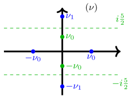
(a)

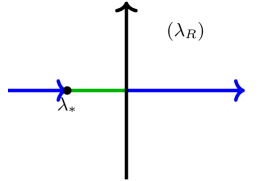
(b)

Figure 6: Fig. (a) gives the solutions for $\nu$ of eq. (30) according the range of $\lambda_{R}$ in fig. (b). $\lambda_{*}$ is the Landau pole.

The non-perturbative OPE coefficient for the $n$-th double trace operator is in turn given by

$$|c(\nu_{n})|^{2}=\stackrel{{\scriptstyle[}}{{\nu}}=\nu_{n}]{}{\text{Res}}\left(\frac{iD^{(\times)}(\nu)}{1-{\mathcal{B}_{\rm ren}}(\nu)}\right).$$ (32)

For $\nu_{0}\to 0_{+}$, $|c(\nu_{0})|^{2}$ grows without bound. We interpret this feature as a manifestation in CFT of the Landau pole of the $\phi^{4}$ theory at negative coupling: The generalized free field represented by a free scalar in AdS₄ is one point in a continuous family of CFT’s which can be parametrized by the bulk coupling $\lambda_{R}$ or, equivalently by the anomalous dimension $\gamma^{(1)}$ in eq. (16). However, when $\gamma^{(1)}=\frac{\lambda_{*}}{32\pi^{2}}$, the spectral representation (3) develops a singularity since the lowest pole crosses the integral contour. This is reminiscent of the Landau pole in $\phi^{4}$ theory which leads to a divergence of loop integrals Landau et al. (1954). Note that while the $\lambda_{R}$-dependence of the double trace dimensions and OPE’s is renormalization scheme dependent the relation between OPE and double trace dimension is not. In CFT one can resolve this singular point by moving the $\nu$ integration contour to the left of this pole and adding the conformal block of this operator by hand, similar to the identity conformal block which was similarly not included in (2) and (3). For the same reason this block has to be removed for the integral in fig. 1 to converge. See Caron-Huot (2017) for a more detailed discussion.

5 Conclusion

A key result in this letter is the renomalized spectral function in eq. (27) which contains all relevant information of the CFT representation of the large-$N$, $O(N)$-model in AdS₄. Other methods have been used for determining the spectral function $\mathcal{B}_{\rm ren}(\nu)$. For instance, in Carmi et al. (2019) the spectral function has been obtained for AdS_d+1 with $d<3$, but the result is not valid for $d\geq 3$ due to the one-loop ultraviolet divergences. Thanks to the AdS invariant regulator Bertan et al. (2019); Heckelbacher and Sachs (2021) the renormalized spectral function is fully determined by the regulated one-loop fish diagram in fig. 4 for which we give a closed form expression in eq. (20).

After extracting the dimensions of the double trace operators and the OPE’s for this spectral function we then found that $\lambda_{R}=\infty$ is not a singular point. However, approaching the Landau pole of the $O(N)$ model in the negative coupling regime a double trace operator of dimension $3/2$ develops a complex dimension which results in a singularity in the spectral representation. The present analysis then shows the appearance of complex dimension operators that translate into a non-unitary CFT everywhere outside the green interval in fig. 6(b), which covers all positive $\lambda_{R}$, in accordance with the tachyonic mode found in Coleman et al. (1974). For a negative coupling $\lambda_{R}\in[\lambda_{*},0]$ the theory is unitary, and the space of couplings is compact. In closing, let us mention that for $\lambda_{R}=\lambda_{*}$ there is a marginal “quadruple trace” operator in the OPE of two double trace operators. It would be interesting to investigate its effect on the CFT and on the bulk theory upon giving to this operator a vacuum expectation value.