Synthetic aperture imaging of dispersive targets

Abstract.

We introduce a dispersive point target model based on scattering by a particle in the far-field. The synthetic aperture imaging problem is then expanded to identify these targets and recover their locations and frequency dependent reflectivities. We show that Kirchhoff migration (KM) is able to identify dispersive point targets in an imaging region. However, KM predicts target locations that are shifted in range from their true locations. We derive an estimate for this range shift for a single target. We also show that because of this range shift we cannot recover the complex-valued frequency dependent reflectivity, but we can recover its absolute value and hence the radar cross-section (RCS) of the target. Simulation results show that we can detect, recover the approximate location, and recover the RCS for dispersive point targets thereby opening opportunities to classifying important differences between multiple targets such as their sizes or material compositions.

Keywords. Synthetic aperture radar, Dispersive targets, Kirchhoff migration, Radar cross-section

1. Introduction

Synthetic aperture radar is an imaging modality in which an airborne antenna is used to collect the reflected signal from a region of interest on the ground. High resolution images are reconstructed by coherently processing the signals along the known flight trajectory [1, 2, 3, 4]. These images provide an estimate of the spatial dependence of the reflectivity often ignoring its frequency content. However, the dispersive nature of the reflectivity of targets is of great interest as it can be helpful for material identification, for example.

A natural approach that has been proposed to that effect is based on dividing the frequency band into sub-bands and then creating an image for each sub-band [5, 6]. Although the individual images have lower resolution, they can be successfully used to provide information about the frequency dependence of the reflectivity. In the same spirit, frequency and direction dependent reflectivity has been successfully reconstructed in [7] using sparsity constraint optimization approaches while dividing the bandwidth and the array aperture in sub-bands and sub-apertures respectively. The reflectivity in this case has a four dimensional parametrization, i.e., space, frequency and direction. Computational complexity limits the applicability of this method for on-the-fly scenarios.

Exploiting Doppler shift in the SAR ambiguity function [1] has been extended to frequency dependent reflectivities and an expression for the SAR point spread function in space and frequency domain has been derived [8]. This point spread function allows for reconstructing an image in which each pixel provides frequency dependent information about the reflectivity [9]. The approach gives promising results but achieving high range resolution remains a challenge.

Another way to account for dispersive targets is to consider the signal in the time domain in which case the scattering delay induced by the target needs to be separated from the propagation delay. This is a challenging problem that has been addressed in [10] provided the synthetic aperture is wide enough. The important question of detectability of this scattering delay in the presence of speckle has been evaluated using statistical divergence measures in [11].

In this paper we consider a realistic model for a frequency dependent reflectivity and propose an imaging method based on coherent back-projection. This method allows us to first image the spatial location of the targets and then determine their frequency dependent reflectivities. High resolution imaging of the target location is obtained using the the tunable synthetic aperture radar imaging approach of [12]. This method relies on a simple mathematical transformation of the classical SAR image depending on a user-defined parameter, $\epsilon$. The resulting image scales the traditional SAR image resolution by $\sqrt{\epsilon}$ thus achieving sub-wavelength target localization.

Due to the frequency dependence of the reflectivity, the target’s location is reconstructed up to a shift in range. Our theoretical analysis provides an estimate of this shift and shows that it is inherently connected to fundamental scattering properties of the target, namely the reflectivity. Once the target location is estimated, the radar cross-section (RCS) of the target can be recovered. Promising results are obtained for single and multiple targets scenarios. Gaining access to RCS information is very important for some remote sensing applications as it provides target classification information in addition to detection and spatial localization.

The remainder of this paper is as follows. In Section 2 we review the elementary theory of scattering by a particle and use that to introduce our dispersive point target model. In Section 3 we describe the SAR imaging problem for dispersive point targets. We apply Kirchhoff migration (KM) to identify the location which, in turn, enables the recovery of the radar cross-section for a single dispersive point target in Section 4. There we show that KM accurately identifies the target location in cross-range, but may produce a shift in range. We derive an estimate for this range shift that identifies the key mechanism producing this shift. We extend these results for multiple targets in Section 5. For that case, we introduce an elementary linear regression problem to obtain the radar cross-sections for each of the targets. In Section 6 we give our conclusions. Appendix A gives a description of scalar wave scattering by a sphere which we use to generate frequency dependent reflectivities used in the simulations results shown here.

2. Scattering by a particle

We briefly review elementary aspects of scattering by a particle and use that to introduce our dispersive point target model. Consider the observation of the scattered field $U_{s}$ at distance $R$ away from a particle with $R>d^{2}/\lambda$ where $d$ is the particle diameter and $\lambda$ the wavelength of the incident light. For this case, the leading behavior of the scattered field is [13]

(1) $$U_{s}\sim f(\hat{\boldsymbol{o}},\hat{\boldsymbol{\imath}};\omega)\frac{e^{\mathrm{i}\omega R/c}}{R}$$

where $\hat{\boldsymbol{o}}$ is the direction of observation, $\hat{\boldsymbol{\imath}}$ is the propagation direction of the incident plane wave, $\omega$ is the frequency and $c$ is the wave speed. The leading behavior given by (1) is a spherical wave modified by $f$, the scattering amplitude. The scattering amplitude contains the amplitude and phase of the scattered field in the far-field at frequency $\omega$.

In synthetic aperture imaging, we measure only the backscattered field corresponding to $\hat{\boldsymbol{o}}=-\hat{\boldsymbol{\imath}}$. The radar cross-section (RCS),

(2) $$\sigma_{\text{RCS}}(\omega)=4\pi|f(-\hat{\boldsymbol{\imath}},\hat{\boldsymbol{\imath}};\omega)|^{2}$$

gives a measure of the power backscattered by the particle. The RCS as a function of $\omega$ depends on the size, shape, and material properties of the particle.

SAR imaging methods such as KM tend to produce images of general objects that exhibit peaks at the most singular portions of those objects, e.g. closest boundaries, corners, etc [3]. For this reason, point target models are commonly used for those imaging problems. The point target model that is typically used for SAR imaging problems assumes that the scattered field measured at a point $\boldsymbol{x}$ is given by

(3) $$U^{s}(\boldsymbol{x})=\rho\frac{e^{\mathrm{i}\omega|\boldsymbol{x}-\boldsymbol{y}|/c}}{4\pi|\boldsymbol{x}-\boldsymbol{y}|}U^{\text{inc}}(\boldsymbol{y}).$$

Here, $U^{\text{inc}}$ is the incident field, $\boldsymbol{y}$ is the location of the point target and $\rho$ is a complex scalar called the reflectivity. Comparing (3) with (1), we see that the reflectivity is the scattering amplitude when $f$ is assumed to be independent of direction and frequency.

We introduce an extension to (3) through inclusion of a frequency dependent reflectivity $\varrho(\omega)$ according to

(4) $$U^{s}(\boldsymbol{x})=\varrho(\omega)\frac{e^{\mathrm{i}\omega|\boldsymbol{x}-\boldsymbol{y}|/c}}{4\pi|\boldsymbol{x}-\boldsymbol{y}|}U^{\text{inc}}(\boldsymbol{y}).$$

We call (4) the dispersive point target model. This model is characterized by the position $\boldsymbol{y}$ and the frequency dependent reflectivity $\varrho(\omega)$.

In the numerical simulations that follow, we determine $\varrho(\omega)$ from the scattering amplitude for a dielectric sphere with radius $\alpha$ and relative refractive index $n_{rel}$ (see Appendix A). Using that reflectivity, we compute the RCS through evaluation of $\sigma_{\text{RCS}}(\omega)=4\pi|\varrho(\omega)|^{2}$.

3. Synthetic aperture imaging

In synthetic aperture radar (SAR) imaging, a single transmitter/receiver is used to collect the scattered electromagnetic field over a synthetic aperture that is created by a moving platform [1, 3, 4]. The moving platform is used to create a suite of experiments in which pulses are emitted and resulting echoes are recorded by the transmitter/receiver at several locations along the flight path. Let $f(t)$ denote the broadband pulse emitted and let $d(s,t)$ denote the data recorded. Here, the measurements depend on the slow time $s$ that parameterizes the flight path of the platform, $\boldsymbol{r}(s)$, and the fast time $t$ in which the round-trip travel time between the platform and the imaging scene on the ground is measured.

High-resolution images of the probed scene can be obtained because the data are coherently processed over a large synthetic aperture created by the moving platform. As illustrated in Fig. 1, the platform is moving along a trajectory probing the imaging scene by sending a pulse $p(t)$ and collecting the corresponding echoes. We call range the direction that is obtained by projecting on the imaging plane the vector that connects the center of the imaging region to the central platform location. Cross-range is the direction that is orthogonal to the range. Denoting the size of the synthetic aperture by $a$ and the available bandwidth by $B$, the typical resolution of the imaging system is $O((c/B)(L/R))$ in range and $O(\lambda_{0}L/a)$ in cross-range. Here $c$ is the speed of light and $\lambda_{0}$ the wavelength corresponding to the central frequency while $L$ denotes the distance between the platform and the imaging region and $R$ the offset in range.

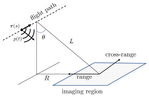
Figure 1. Synthetic aperture radar imaging schematic.

In what follows, we use the start-stop approximation which neglects displacements of the platform and targets in comparison with the propagation of signals emitted and received on the platform. Let $\boldsymbol{x}_{n}$ for $n=1,\dots,N$ denote the positions of the emitter/receiver along the flight path making up a synthetic aperture. The imaging system operates with frequencies $\omega_{m}$ for $m=1,\dots,M$ sampling the system bandwidth, $2\pi B$.

Suppose there is dispersive point target located at $\boldsymbol{y}_{0}$, a point in the imaging region, with frequency dependent reflectivity, $\varrho_{0}(\omega)$. When the signal is emitted from the emitter/receiver, it propagates into the medium, is incident on the dispersive point target and scatters. The field scattered by the dispersive point target is then measured on the emitter/receiver. The resulting measurement of the scattered field by the emitter/receiver due to an isotropic and flat frequency point source at $\boldsymbol{x}_{n}$ is

(5) $$d_{mn}=\varrho_{0}(\omega_{m})\frac{e^{\mathrm{i}2\omega_{m}|\boldsymbol{x}_{n}-\boldsymbol{y}_{0}|/c}}{(4\pi|\boldsymbol{x}_{n}-\boldsymbol{y}_{0}|)^{2}},\quad m=1,\dots,M,\quad n=1,\dots,N.$$

The matrix $D\in\mathbb{C}^{M\times N}$ whose entries are given by (5) contains the measurements.

The imaging problem is to determine the locations of targets and the frequency dependent reflectivity in some specified imaging region. We show below that we cannot recover the frequency dependent reflectivity, in general. Instead we seek to recover the RCS for each of the targets.

In the simulations results that follow, we use system parameters based on the GOTCHA data set [14]. In particular, we have set $R=3.55\,\text{km}$ and $H=7.30\,\text{km}$, so that $L=\sqrt{H^{2}+R^{2}}=8.12\,\text{km}$. The synthetic aperture created by the linear flight path is $a=0.13\,\text{km}$. The central frequency is $\omega_{0}/(2\pi)=9.6\,\text{GHz}$ and the bandwidth is $B=622\,\text{MHz}$. Using $c=3\times 10^{8}\,\text{m/s}$, we find that the central wavelength is $\lambda_{0}=3.12\,\text{cm}$. The imaging region is at the ground level $z=0$. We use $M=25$ equi-spaced frequencies sampling the bandwidth, and $N=32$ equi-spaced spatial measurements sampling the synthetic aperture.

4. KM for a single dispersive point target

Let $\boldsymbol{y}$ denote a point in the imaging region. We consider the image formed through evaluation of the KM imaging function,

(6) $$I^{\text{KM}}(\boldsymbol{y})=\sum_{m=1}^{M}\sum_{n=1}^{N}d_{mn}e^{-\mathrm{i}2\omega_{m}|\boldsymbol{x}_{n}-\boldsymbol{y}|/c}.$$

Note that in (6), the entries of the data matrix are back-propagated to $\boldsymbol{y}$ through multiplication by $e^{-\mathrm{i}2\omega_{m}|\boldsymbol{x}_{n}-\boldsymbol{y}|/c}$. Those results are summed over spatial locations (sum in $n$) and frequencies (sum in $m$). Through evaluation of this KM imaging function over a set of points and plotting those results, we produce an image of targets in the imaging region.

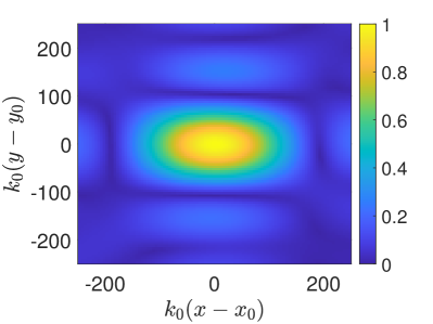
Figure 2. Evaluation of (6) on an imaging region that is $500/k_{0}\times 500/k_{0}$ centered about the target location $(x_{0},y_{0})$ with $k_{0}$ denoting the central wavenumber. The reflectivity was computed for a sphere with $k_{0}\alpha=1.4$ and $n_{rel}=1.4$. Measurement noise was added so that $\text{SNR}=3.73$ dB.

In Fig. 2 we show the result of evaluating (6) for a dispersive point target located at $(k_{0}x_{0},k_{0}y_{0})=(273.713,-346.167)$ over a $500/k_{0}\times 500/k_{0}$ imaging region. The reflectivity was computed for a sphere with $k_{0}\alpha=1.4$ and $n_{rel}=1.4$. Measurement noise was added so that $\text{SNR}=3.73$ dB. The image shown in Fig. 2 shows $I^{\text{KM}}$ normalized by its maximum value. This image indicates the presence of a target through its peak. The location of the peak predicts the location of the target. Away from the peak, we observe imaging artifacts as sidelobes to the peak.

We have recently introduced a modification to KM that produces tunably high-resolution images [12]. Let $\tilde{I}^{\text{KM}}$ denote (6) normalized by its maximum as shown in Fig. 2. The modification to KM simply requires evaluation of

(7) $$I_{\epsilon}^{\text{KM}}=\frac{\epsilon}{1-(1-\epsilon)\tilde{I}^{\text{KM}}},$$

with $\epsilon$ denoting a user-defined parameter. The resolution of the resulting image produced using (7) scales with $\sqrt{\epsilon}$.

When we plot $I_{\epsilon}^{\text{KM}}$ with $\epsilon=10^{-4}$ using the image shown in Fig. 2, we obtain the image shown in Fig. 3. Note that the region plotted is $20/k_{0}\times 20/k_{0}$, which is a much smaller region than that plotted in Fig. 2. This result shows that this modified KM method is able to image targets with subwavelength resolution. Moreover, since the parameter $\epsilon$ is user-defined, this high resolution is tunable.

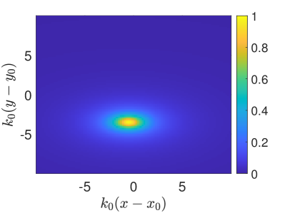
Figure 3. Evaluation of the modified KM given in (7) with $\epsilon=10^{-4}$ applied to the image shown in Fig. 2 on an imaging region that is $20/k_{0}\times 20/k_{0}$ centered about the target location $(x_{0},y_{0})$.

4.1. Range shift

Because of the high-resolution capabilities of the modified KM method, we are able to observe that the predicted target location is shifted from the exact location, especially in range. The peak of the image shown in Fig. 3 is located at $(k_{0}\hat{x},k_{0}\hat{y})=(273.113,-349.770)$ compared to the true location at $(k_{0}x_{0},k_{0}y_{0})=(273.713,-346.167)$. In simulations, we find that if the SNR is larger, the cross-range coordinate $x_{0}$ becomes exact. However, the range coordinate $y_{0}$ remains shifted. For example, with $\text{SNR}=13.73$ dB we obtain a predicted target location at $(k_{0}\hat{x},k_{0}\hat{y})=(273.713,-350.170)$, and with $\text{SNR}=23.73$ dB, we obtain a predicted target location at $(k_{0}\hat{x},k_{0}\hat{y})=(273.713,-350.170)$. We find that this shift in the predicted range of the target varies with both the size parameter, $k_{0}\alpha$, and the relative refractive index, $n_{rel}$ used to generate the frequency dependent reflectivity.

To understand the cause of this shift in the range coordinate, we substitute (5) into (6) and obtain

(8) $$I^{\text{KM}}(\boldsymbol{y})=\sum_{m=1}^{M}\varrho_{0}(\omega_{m})\sum_{n=1}^{N}\frac{e^{\mathrm{i}2\omega_{m}(|\boldsymbol{x}_{n}-\boldsymbol{y}_{0}|-|\boldsymbol{x}_{n}-\boldsymbol{y}|)/c}}{(4\pi|\boldsymbol{x}_{n}-\boldsymbol{y}_{0}|)^{2}}.$$

Consider a coordinate system in which the origin lies at the center of the imaging region. The coordinates of the spatial measurements are $\boldsymbol{x}_{n}=(\xi_{n},R,H)$ for $n=1,\dots,N$ with $\xi_{n}=-a/2+a(n-1)/(N-1)$. We write $\boldsymbol{y}_{0}=(x_{0},y_{0},0)$ and $\boldsymbol{y}=(x_{0},y_{0}+y,0)$. Let $\theta$ denote the look angle (see Fig. 1) so that $R=L\sin\theta$ and $H=L\cos\theta$. In the asymptotic limit $L\to\infty$, we find that

(9) $$|\boldsymbol{x}_{n}-\boldsymbol{y}_{0}|-|\boldsymbol{x}_{n}-\boldsymbol{y}|=y\sin\theta+O(L^{-1}).$$

It follows that

(10) $$I^{\text{KM}}\sim\frac{N}{(4\pi L)^{2}}\sum_{m=1}^{M}\varrho_{0}(\omega_{m})e^{\mathrm{i}2\omega_{m}y\sin\theta/c},$$

in this asymptotic limit.

Let

(11) $$a(y)=\sum_{m=1}^{M}\varrho_{m}e^{\mathrm{i}2k_{m}y\sin\theta},$$

with $\varrho_{m}=\varrho_{0}(\omega_{m})$ and $k_{m}=\omega_{m}/c$. Using

(12) $$k_{m}=k_{0}+\frac{2\pi B}{c}\left(-\frac{1}{2}+\frac{m-1}{M-1}\right),$$

for $m=1,\dots,M,$ with $k_{0}$ denoting the central wavenumber, we introduce the scaled variable $y\sin\theta=2\pi BY/c$ and consider instead

(13) $$a\left(\frac{2\pi B}{c\sin\theta}Y\right)=e^{\mathrm{i}2\kappa_{0}Y}A(Y),$$

where

(14) $$A(Y)=\sum_{m=1}^{M}\varrho_{m}\exp\left[\mathrm{i}\left(-1+2\frac{m-1}{M-1}\right)Y\right],$$

and $\kappa_{0}=k_{0}\sin\theta c/(2\pi B)$.

In what follows, we make use of the following identity

(15) $$\sum_{m=r+1}^{M}\exp\left[\mathrm{i}\left(-1+2\frac{m-1}{M-1}\right)Y\right]=e^{\mathrm{i}rY/(M-1)}\Psi_{r}^{M}(Y).$$

where

(16) $$\Psi_{r}^{M}(Y)=\frac{\sin\left(\frac{M-r}{M-1}Y\right)}{\sin\left(\frac{Y}{M-1}\right)}.$$

The function $\Psi_{r}^{M}(Y)$ is real and even, and it attains its maximum of $M-r$ on $Y=0$. When we apply the summation by parts formula,

(17) $$\sum_{m=1}^{M}u_{m}v_{m}=u_{1}\sum_{m=1}^{M}v_{m}-\sum_{r=1}^{M-1}(u_{r+1}-u_{r})\sum_{m=r+1}^{M}v_{m},$$

to (14), we find that

(18) $$A(Y)=\sum_{m=1}^{M}\varDelta\varrho_{m}e^{\mathrm{i}(m-1)Y/(M-1)}\Psi_{m-1}^{M}(Y),$$

with $\varDelta\varrho_{m}=\varrho_{m+1}-\varrho_{m}$ and $\varrho_{0}\equiv 0$. It follows that

(19) $$|A(Y)|^{2}=\sum_{m=1}^{M}|\varDelta\varrho_{m}|^{2}(\Psi_{m-1}^{M}(Y))^{2}+2\sum_{m=1}^{M-1}\sum_{r=m+1}^{M}\bigg{\{}\text{Re}\left[\varDelta\varrho_{m}^{\ast}\varDelta\varrho_{r}\right]\cos\left(\frac{r-m}{M-1}Y\right)\Psi_{m-1}^{M}(Y)\Psi_{r-1}^{M}(Y)\bigg{\}}\\ -2\sum_{m=1}^{M-1}\sum_{r=m+1}^{M}\bigg{\{}\text{Im}\left[\varDelta\varrho_{m}^{\ast}\varDelta\varrho_{r}\right]\sin\left(\frac{r-m}{M-1}Y\right)\Psi_{m-1}^{M}(Y)\Psi_{r-1}^{M}(Y)\bigg{\}}.$$

Note that in (19) the first two sums are even functions of $Y$ and the third sum is odd in $Y$. That third sum plays a key role in the range shift.

To compute an estimate for where $|A(Y)|^{2}$ attains its maximum, we expand the functions of $Y$ in each of the three sums in (19) about $Y=0$ and keep terms up to $O(Y^{2})$. Combining these results yields a quadratic approximation for $|A(Y)|^{2}$. By computing the critical point of this quadratic approximation, we find that this approximation attains its maximum on $\hat{Y}=-3(M-1)\alpha_{1}/\alpha_{2}$ where

(20) $$\alpha_{1}=\sum_{m=1}^{M-1}\sum_{r=m+1}^{M}\text{Im}[\varDelta\varrho_{m}\varDelta\varrho_{r}](r-m)(M-m+1)(M-r+1),$$

and

(21) $$\alpha_{2}=\sum_{m=1}^{M}|\varDelta\varrho_{m}|^{2}\left[(M-m+1)^{4}-(M-m+1)^{2}\right]\\ +\sum_{m=1}^{M-1}\sum_{r=m+1}^{M}\text{Re}[\varDelta\varrho_{m}^{\ast}\varDelta\varrho_{r}]\left(M^{2}+2M-3mr+m(2m-M-1)+r(2r-M-1)\right).$$

This critical point $\hat{Y}$ gives an estimate for the range shift of the target location predicted by KM. We show a comparison of the numerically determined location of the predicted target and this estimate in Fig. 4. This comparison is done using the frequency dependent reflectivity of a sphere with relative refractive index $1.4$ for various non-dimensional sizes, $k_{0}\alpha$.

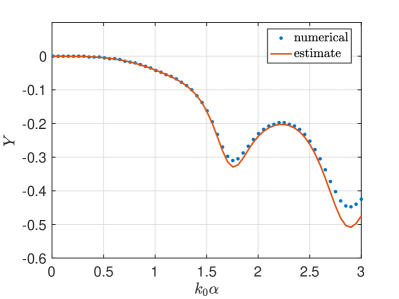
Figure 4. A comparison of the range coordinate of the target predicted using KM (numerical), and by computing the estimate $\hat{Y}$ (estimate) over reflectivities computed using spheres with $n_{rel}=1.4$ over a range of different sizes, $k_{0}\alpha$.

These results show that the estimate accurately captures the behavior of this range shift over a broad range of sphere sizes. However, the error of this estimate grows with the sphere size, but especially where the range shift oscillates. These oscillations are presumably due to the complex scattering behavior of large spheres ($k_{0}\alpha>1$) that exhibit phenomena such as Mie resonances. In Fig. 5 we show the RCS evaluated on the central frequency $\omega_{0}$ normalized by the geometric cross-section, $\sigma_{g}=\pi\alpha^{2}$ for spheres with $n_{rel}=1.4$ over the same range of $k_{0}\alpha$ plotted in Fig. 4. Note that the behavior of the range shifts shown in Fig. 4 closely follow the behavior of the RCS shown in Fig. 5. In this way, we see that the range shift in the predicted range of the target by KM is inherently connected to fundamental scattering properties of the target.

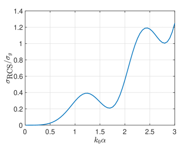
Figure 5. The RCS $\sigma_{\text{RCS}}$ normalized by the geometric cross-section $\sigma_{g}=\pi\alpha^{2}$ evaluated on the central frequency $\omega_{0}$ for spheres with $n_{rel}=1.4$ over a range of sphere sizes $k_{0}\alpha$.

4.2. Radar cross-section

We now seek to recover $\varrho(\omega_{m})$ for $m=1,\dots,M$. Suppose we have evaluated (6) and produced an image that identifies a target and its predicted location, $\hat{\boldsymbol{y}}_{0}$. We evaluate

(22) $$\phi_{m}=\frac{1}{N}\sum_{n=1}^{N}d_{mn}(4\pi|\boldsymbol{x}_{n}-\hat{\boldsymbol{y}}_{0}|)^{2}e^{-\mathrm{i}2\omega_{m}|\boldsymbol{x}_{n}-\hat{\boldsymbol{y}}_{0}|/c},$$

for $m=1,\dots,M$. Substituting (5) into (22) yields

(23) $$\phi_{m}=\varrho_{0}(\omega_{m})\frac{1}{N}\sum_{n=1}^{N}\frac{|\boldsymbol{x}_{n}-\hat{\boldsymbol{y}}_{0}|^{2}}{|\boldsymbol{x}_{n}-\boldsymbol{y}_{0}|^{2}}e^{\mathrm{i}2\omega_{m}\varDelta\tau_{n}},$$

with $\varDelta\tau_{n}=(|\boldsymbol{x}_{n}-\boldsymbol{y}_{0}|-|\boldsymbol{x}_{n}-\hat{\boldsymbol{y}}_{0}|)/c$.

In the asymptotic limit $L\to\infty$, we find using the same expansions used above that

(24) $$\phi_{m}\sim\varrho_{0}(\omega_{m})e^{\mathrm{i}2\omega_{m}\varDelta y\sin\theta/c},$$

for $m=1,\dots,M$. Here, $\varDelta y$ denotes the range shift associated with the predicted location $\hat{\boldsymbol{y}}_{0}$. Because the range shift $\varDelta y$ is not known, we cannot remove the factor of $e^{\mathrm{i}2\omega_{m}\varDelta y\sin\theta/c}$ from the expression above. Therefore, we cannot recover the complex values of $\varrho_{0}(\omega_{m})$. However, we find that

(25) $$|\phi_{m}|^{2}\sim|\varrho_{0}(\omega_{m})|^{2}.$$

Therefore, we recover the RCS given the predicted location of the target by KM through evaluation of

(26) $$\hat{\sigma}_{\text{RCS}}(\omega_{m})=4\pi|\phi_{m}|^{2}.$$

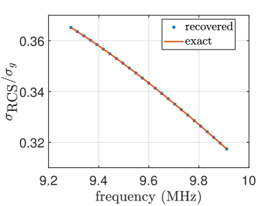
Figure 6. The recovered RCS using (26) normalized by the geometric cross-section $\sigma_{g}=\pi\alpha^{2}$ for the reflectivity used in Figs. 2 and 3 corresponding to $k_{0}\alpha=1.4$ and $n_{rel}=1.4$. To compute $\hat{\sigma}_{\text{RCS}}(\omega)$, we estimate $\hat{\boldsymbol{y}}_{0}$ by finding where $I_{\epsilon}^{\text{KM}}$ attains its maximum value on the mesh used for plotting.

In Fig. 6 we show the estimated RCS using (26) for the same data used in Figs. 2 and 3. To estimate $\hat{\boldsymbol{y}}_{0}$ we use the mesh location used to plot those images where $I_{\epsilon}^{\text{KM}}$ attains its maximum value which is $(\hat{x},\hat{y})=(1.357,-1.738)$ cm compared to the true location $(x_{0},y_{0})=(1.360,-1.720)$ cm. The exact RCS computed from the reflectivity is plotted for comparison. The estimated RCS is indistinguishable from the exact RCS and the relative error is on the order of $10^{-4}$.

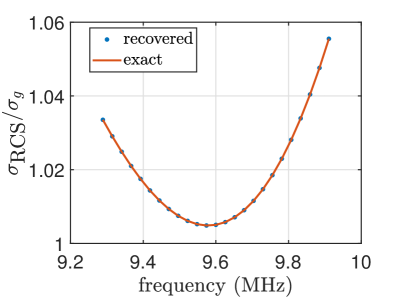
Figure 7. The recovered RCS using (26) normalized by the geometric cross-section $\sigma_{g}=\pi\alpha^{2}$ for the reflectivity corresponding to $k_{0}\alpha=2.8$ and $n_{rel}=1.4$. To compute $\hat{\sigma}_{\text{RCS}}(\omega)$, we estimate $\hat{\boldsymbol{y}}_{0}$ by finding where $I_{\epsilon}^{\text{KM}}$ attains its maximum value on the mesh used for plotting.

We consider a target whose reflectivity is computed for a sphere of size $k_{0}\alpha=2.8$ and relative refractive index $n_{rel}=1.4$. Measurement noise was added so that $\text{SNR}=3.72$ dB. The location predicted by finding the mesh point on which $I_{\epsilon}^{\text{KM}}$ attains its maximum is $(\hat{x},\hat{y})=(1.358,-1.797)$ cm. We estimate the RCS through evaluation of (26) using this predicted target location. The results are plotted in Fig. 7. Note that the RCS for this problem is markedly different from that shown in Fig. 6. Nonetheless, the estimated RCS is still accurate with a relative error on the order of $10^{-5}$.

5. Multiple targets

Suppose now the imaging region contains $Q$ dispersive point targets at locations $\boldsymbol{y}_{q}$ with reflectivities $\varrho_{q}(\omega)$ for $q=1,\dots,Q$. Assuming that these targets scatter independently, measurements are modeled according to

(27) $$d_{mn}=\sum_{q=1}^{Q}\varrho_{q}(\omega_{m})\frac{e^{\mathrm{i}2\omega_{m}|\boldsymbol{x}_{n}-\boldsymbol{y}_{q}|/c}}{(4\pi|\boldsymbol{x}_{n}-\boldsymbol{y}_{q}|)^{2}}.$$

From our results for a single target, we anticipate that evaluating the KM imaging function given in (6) will identify and locate targets under the condition that these targets are not too close to one another as measured with respect to the resolution produced by KM for a single target.

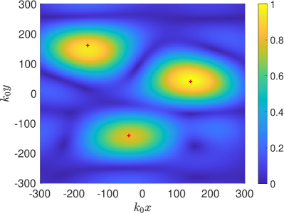
Figure 8. Imaged produced by KM through evaluation of (6) over an imaging region containing 3 dispersive point targets whose exact locations are plotted as red “+” symbols.

In Fig. 8 we show a result of evaluating (6) over an imaging region containing three different dispersive point targets. The first target is located at $(k_{0}x_{1},k_{0}y_{1},k_{0}z_{1})=(140.882,40.252,0)$. Its reflectivity $\varrho_{1}(\omega)$ is computed using a sphere of size $k_{0}\alpha_{1}=0.8$ and relative refractive index $n_{rel,1}=1.8$. The second target is located at $(k_{0}x_{2},k_{0}y_{2},k_{0}z_{2})=(-40.252,-140.882,0)$. Its reflectivity $\varrho_{2}(\omega)$ is computed using a sphere of size $k_{0}\alpha_{1}=1.2$ and relative refractive index $n_{rel,2}=1.4$. The third target is located at $(k_{0}x_{3},k_{0}y_{3},k_{0}z_{3})=(-161.008,161.008,0)$. Its reflectivity $\varrho_{3}(\omega)$ is computed using a sphere of size $k_{0}\alpha_{3}=1.8$ and relative refractive index $n_{rel,3}=1.4$. Measurement noise was added to the data so that $\text{SNR}=22.84$ dB. Figure 8 shows three distinct peaks in the vicinity of the three targets whose locations are plotted as red “+” symbols.

To obtain high-resolution images of individual targets, we consider $50/k_{0}\times 50/k_{0}$ sized sub-regions about each of the peaks shown in Fig. 8. We normalize the portion of the image contained in each of those sub-regions so that the maximum value contained in that sub-region is unity. Then we apply (7) with $\epsilon=10^{-4}$. Those results appear in Fig. 9.

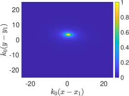
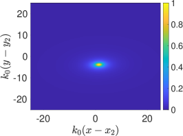
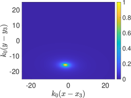
Figure 9. Images produced using modified KM given in (7) in $50/k_{0}\times 50/k_{0}$ sub-regions centered about each of the exact target locations. The left plot corresponds to target 1, the center plot corresponds to target 2 and the right plot corresponds to target 3.

The modified KM images produce high resolution images of the targets. However, we observed that the predicted target locations are shifted in both range and cross-range from the exact target locations. The predicted location for target 1 is $(k_{0}\hat{x}_{1},k_{0}\hat{y}_{1})=(141.382,43.502)$, for target 2 is $(k_{0}\hat{x}_{2},k_{0}\hat{y}_{2})=(-39.002,-144.882)$, and for target 3 is $(k_{0}\hat{x}_{3},k_{0}\hat{y}_{3})=(-162.758,145.008)$. These shifts in the predictions from the exact locations are approximately $2\lambda_{0}$.

To understand why these shifts in predicted target locations occur in both range and cross-range, suppose we evaluate (6) on $\boldsymbol{y}_{1}$, the exact location for target one. The result is

(28) $$I^{\text{KM}}(\boldsymbol{y}_{1})=\sum_{m=1}^{M}\sum_{n=1}^{N}\left[\frac{\varrho_{1}(\omega_{m})}{(4\pi|\boldsymbol{x}_{n}-\boldsymbol{y}_{1}|)^{2}}+\sum_{q=2}^{Q}\varrho_{q}(\omega_{m})\frac{|\boldsymbol{x}_{n}-\boldsymbol{y}_{1}|^{2}}{|\boldsymbol{x}_{n}-\boldsymbol{y}_{q}|^{2}}e^{\mathrm{i}2\omega_{m}\varDelta\tau_{1q}^{n}}\right],$$

where $\varDelta\tau_{pq}^{n}=(|\boldsymbol{x}_{n}-\boldsymbol{y}_{q}|-|\boldsymbol{x}_{n}-\boldsymbol{y}_{p}|)/c$. From this result we see that in addition to the contribution made by target 1, we obtain small, but non-trivial contributions by all other targets, each of which carries a phase associated with $\varDelta\tau_{q,p}^{n}$. Therefore, upon computing $|I^{\text{KM}}|$, those phases mix leading to shifts in the predicted target positions.

Even though the predicted locations of targets are not exact, we seek to recover the RCS of each of the targets. Let $\hat{\boldsymbol{y}}_{p}$ denote the approximate location of target $p$. Let

(29) $$\phi_{m}(\hat{\boldsymbol{y}}_{p})=\frac{1}{N}\sum_{n=1}^{N}d_{mn}(4\pi|\boldsymbol{x}_{n}-\hat{\boldsymbol{y}}_{p}|)^{2}e^{-\mathrm{i}2\omega_{m}|\boldsymbol{x}_{n}-\hat{\boldsymbol{y}}_{p}|/c}.$$

Substituting (27) into this expression, we obtain

(30) $$\phi_{m}(\hat{\boldsymbol{y}}_{p})=\sum_{q=1}^{Q}a_{pq}(\omega_{m})\varrho_{q}(\omega_{m}),$$

where

(31) $$a_{pq}(\omega_{m})=\frac{1}{N}\sum_{n=1}^{N}\frac{|\boldsymbol{x}_{n}-\hat{\boldsymbol{y}}_{p}|^{2}}{|\boldsymbol{x}_{n}-\boldsymbol{y}_{q}|^{2}}e^{\mathrm{i}2\omega_{m}\varDelta\hat{\tau}_{q,p}^{n}},$$

and $\varDelta\hat{\tau}_{pq}^{n}=(|\boldsymbol{x}_{n}-\boldsymbol{y}_{q}|-|\boldsymbol{x}_{n}-\hat{\boldsymbol{y}}_{p}|)/c$. Equation (30) is a linear system for the unknown reflectivities $\varrho_{q}(\omega_{m})$. Although $a_{pq}(\omega_{m})$ uses the predicted target position $\hat{\boldsymbol{y}}_{p}$, it uses the exact target positions $\boldsymbol{y}_{q}$. Since we do not have access to those exact target locations, we instead consider the linear system,

(32) $$\phi_{m}(\hat{\boldsymbol{y}}_{p})=\sum_{q=1}^{Q}\tilde{a}_{pq}(\omega_{m})\tilde{\varrho}_{q}(\omega_{m}),$$

where

(33) $$\tilde{a}_{pq}(\omega_{m})=\frac{1}{N}\sum_{n=1}^{N}\frac{|\boldsymbol{x}_{n}-\hat{\boldsymbol{y}}_{p}|^{2}}{|\boldsymbol{x}_{n}-\hat{\boldsymbol{y}}_{q}|^{2}}e^{\mathrm{i}2\omega_{m}\varDelta\tilde{\tau}_{q,p}^{n}},$$

with $\varDelta\tilde{\tau}_{pq}^{n}=(|\boldsymbol{x}_{n}-\hat{\boldsymbol{y}}_{q}|-|\boldsymbol{x}_{n}-\hat{\boldsymbol{y}}_{p}|)/c$, and

(34) $$\tilde{\varrho}_{q}(\omega_{m})=\varrho_{q}(\omega_{m})\frac{|\boldsymbol{x}_{n}-\hat{\boldsymbol{y}}_{q}|^{2}}{|\boldsymbol{x}_{n}-\boldsymbol{y}_{q}|^{2}}e^{\mathrm{i}\omega_{m}(\varDelta\tau_{pq}^{n}-\varDelta\hat{\tau}_{pq}^{n})}.$$

When the predicted target locations are close, we expect that $|\boldsymbol{x}_{n}-\hat{\boldsymbol{y}}_{q}|^{2}/|\boldsymbol{x}_{n}-\boldsymbol{y}_{q}|^{2}\approx 1$. The difference in phase, $\varDelta\tau_{pq}^{n}-\varDelta\hat{\tau}_{pq}^{n}$, may be significant, so we expect that we will not be able to recover $\varrho_{q}(\omega_{m})$ from $\tilde{\varrho}_{q}(\omega_{m})$. However, in the asymptotic limit as $L\to\infty$, we find that the RCS for the $q$th target is

(35) $$\sigma_{\text{RCS},q}(\omega_{m})=4\pi|\tilde{\varrho}_{q}(\omega_{m})|^{2}+O(L^{-1}).$$

Hence, we use this leading behavior to estimate the RCS of the targets.

To summarize, we give the following procedure for estimating the RCS for each of the targets identified in the imaging region.

1. Evaluate (6) over the imaging region to identify targets.

2. Evaluate (7) in sub-regions to estimate the locations of individual targets.

3. Solve the linear system (32) and obtain $\tilde{\varrho}_{q}(\omega_{m})$ for $q=1,\dots,Q$ and $m=1,\dots,M$.

4. Evaluate (35) to obtain estimates for the RCS for each of the $Q$ targets.

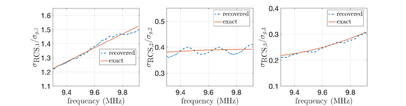
Figure 10. The recovered RCS for the three targets normalized by the corresponding geometric cross-section for the three targets whose location is recovered from Fig 7. Data with $\text{SNR}=22.84$ dB. The left plot corresponds to target 1, the center plot corresponds to target 2 and the right plot corresponds to target 3.

The results for the recovered RCS for the three targets shown in Figs. 8 and 9 are shown in Fig. 10. These results are more noisy than the ones obtained for the single target case but their accuracy is still sufficient to help us characterize targets of different materials/size. As the SNR of data decreases, the locations of the targets are recovered with the same precision but the recovered RCS’s are more noisy. For data with $\text{SNR}=12.84$ dB, the predicted location for target 1 is $(k_{0}\hat{x}_{1},k_{0}\hat{y}_{1})=(141.632,43.002)$, for target 2 is $(k_{0}\hat{x}_{2},k_{0}\hat{y}_{2})=(-39.502,-144.632)$, and for target 3 is $(k_{0}\hat{x}_{3},k_{0}\hat{y}_{3})=(-163.508,145.508)$ and the recovered RCS are shown in Figure 11.

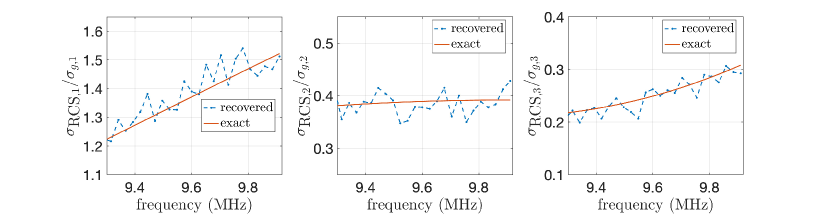
Figure 11. The recovered RCS for the three targets normalized by the corresponding geometric cross-section. Data with $\text{SNR}=12.84$ dB. The left plot corresponds to target 1, the center plot corresponds to target 2 and the right plot corresponds to target 3.

We observe in Fig. 11 that the recovered RCS oscillates due to the measurement noise. A smoothing estimate can be obtained using quadratic regression as illustrated by the results in Fig. 12. Those smoothed results effectively capture the behaviors of the RCS for the individual targets.

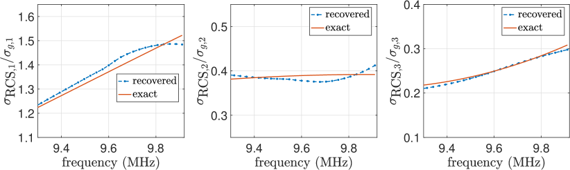
Figure 12. The recovered RCS for the three targets normalized by the corresponding geometric cross-section. Data with $\text{SNR}=12.84$ dB. Smoothing using quadratic regression over the results shown in Fig 9. The left plot corresponds for target 1, the center plot corresponds to target 2 and the right plot corresponds to target 3.

6. Conclusions

We have introduced a dispersive point target model in which the reflectivity is dependent on frequency. We have used scalar wave scattering by a dielectric sphere to model targets of different sizes and materials. Then we have applied KM and our recent modification to KM to obtain high-resolution images of dispersive point targets from SAR measurements. For a single dispersive point target, we observe a shift in the predicted location of the target in the range coordinate. We have computed an accurate estimate for this range shift which is in terms of the frequency dependent reflectivity. Despite the range shift in the predicted location of a single dispersive point target, we are able to recover its radar cross-section (RCS) using that prediction.

When we apply KM and its modification to an imaging region containing multiple dispersive point targets, we find that we can image each of the target locations provided that they are far enough apart from one another with respect to the resolution of KM. We have shown that our modification to KM works in sub-regions that isolate an individual target. Those high resolution images of individual targets reveal that the predicted locations of the targets are shifted in range and cross-range. To recover the RCS for each of the targets, we introduce a linear system using the predicted locations. Our numerical results show that the recovery of RCS’s for multiple targets is much more sensitive to noise. By applying smoothing to those RCS results, we obtain good approximations that allow one to distinguish qualitative differences between the different targets.

By introducing the dispersive point target model and developing methods for imaging dispersive point targets, we have opened opportunities for target classification. Indeed, by recovering the RCS as a function of frequency, we may be able to distinguish targets with different characteristics such as sizes or material properties. We believe that this opportunity to classify in addition to target detection and locatization is useful for a broad variety of SAR imaging applications.

Appendix A Scalar wave scattering by a sphere

We briefly describe scalar wave scattering by a sphere and explain how we generated different frequency dependent reflectivities from this problem. For a fixed frequency, let $k_{0}$ denote the wavenumber in the exterior to a sphere of radius $\alpha$ and $k_{1}=k_{0}n_{rel}$ denote the wavenumber interior to that sphere. A plane wave is incident on the sphere in direction $\hat{\boldsymbol{\imath}}$, which we denote by $U_{i}$. The scattered field exterior to the sphere is

(36) $$U_{s}(R,\hat{\boldsymbol{o}})=\sum_{n=0}^{\infty}a_{n}h_{n}^{(1)}(k_{0}R)P_{n}(\hat{\boldsymbol{\imath}}\cdot\hat{\boldsymbol{o}}),$$

with $h_{n}^{(1)}$ denoting the spherical Hankel function of the first kind with order $n$, and $P_{n}$ denoting the Legendre polynomial of order $n$. The field interior to the sphere is

(37) $$U_{int}(R,\hat{\boldsymbol{o}})=\sum_{n=0}^{\infty}b_{n}j_{n}(k_{0}R)P_{n}(\hat{\boldsymbol{\imath}}\cdot\hat{\boldsymbol{o}}),$$

with $j_{n}$ denoting the spherical Bessel function. We determine the expansion coefficients $a_{n}$ and $b_{n}$ by requiring that $U_{i}+U_{s}=U_{int}$ and $\partial_{r}U_{i}+\partial_{r}U_{s}=\partial_{r}U_{int}$ on $R=\alpha$. We compute a numerical approximation by truncating the series at $n=32$ and making use of the orthogonal properties of Legendre polynomials.

Using the asymptotic behavior $h_{n}^{(1)}(z)\sim\mathrm{i}^{-n-1}z^{-1}e^{\mathrm{i}z}$ as $z\to\infty$, we find that

(38) $$U_{s}(R,\hat{\boldsymbol{o}})\sim\left[\frac{1}{k_{0}}\sum_{n=0}^{\infty}a_{n}\mathrm{i}^{-n-1}P_{n}(\hat{\boldsymbol{\imath}}\cdot\hat{\boldsymbol{o}})\right]\frac{e^{\mathrm{i}k_{0}R}}{R},$$

in the asymptotic limit, $R\to\infty$. The bracketed term in the expression above gives the scattering amplitude $f$. Next, we use $P_{n}(-1)=(-1)^{n}$ to determine that

(39) $$f(\hat{\boldsymbol{\imath}},-\hat{\boldsymbol{\imath}})=\frac{1}{k_{0}}\sum_{n=0}^{\infty}(-1)^{n}\mathrm{i}^{-n-1}a_{n}.$$

We approximate this scattering amplitude by truncating the series as we have done to determine the expansion coefficients. That result is used as our frequency dependent reflectivity. We compute different reflectivities by specifying different values of the radius $\alpha$ and the reflective index $n_{rel}$.

Acknowlegments

This work was supported by the AFOSR Grant FA9550-21-1-0196. A. D. Kim also acknowledges support by NSF Grant DMS-1840265).

References

- [1] M. Cheney, “A mathematical tutorial on synthetic aperture radar,” SIAM Review, vol. 43, no. 2, pp. 301–312, 2001.
- [2] I. G. Cumming and F. H. Wong, Digital Processing of Synthetic Aperture Radar Data: Algorithms and Implementation. Artech House, Boston MA, 2005.
- [3] M. Cheney and B. Borden, Fundamentals of Radar Imaging. SIAM, 2009, vol. 79.
- [4] A. Moreira, P. Prats-Iraola, M. Younis, G. Krieger, I. Hajnsek, and K. P. Papathanassiou, “A tutorial on synthetic aperture radar,” IEEE Geosci. Remote Sens. Mag., vol. 1, no. 1, pp. 6–43, 2013.
- [5] P. Sotirelis, J. T. Parker, M. Fu, X. Hu, and R. Albanese, “A study of material identification using SAR,” in 2012 IEEE Radar Conference, 2012, pp. 0112–0115.
- [6] R. A. Albanese and R. L. Medina, “Materials identification synthetic aperture radar: progress toward a realized capability,” Inverse Probl., vol. 29, p. 054001, 2013.
- [7] L. Borcea, M. Moscoso, G. Papanicolaou, and C. Tsogka, “Synthetic aperture imaging of direction-and frequency-dependent reflectivities,” SIAM J. Imaging Sci., vol. 9, no. 1, pp. 52–81, 2016.
- [8] M. Cheney, “Imaging frequency-dependent reflectivity from synthetic-aperture radar,” Inverse Probl., vol. 29, p. 054002, 2013.
- [9] P. Sotirelis, J. Parker, X. Hu, M. Cheney, and M. Ferrara, “Frequency-dependent reflectivity image reconstruction,” in Algorithms for Synthetic Aperture Radar Imagery XX, E. Zelnio and F. D. Garber, Eds., vol. 8746, International Society for Optics and Photonics. SPIE, 2013, p. 874602. [Online]. Available: https://doi.org/10.1117/12.2020647
- [10] M. Gilman and S. Tsynkov, “Detection of delayed target response in SAR,” Inverse Probl., vol. 35, p. 085005, 2019.
- [11] ——, “Divergence measures and detection performance for dispersive targets in SAR,” Radio Science, vol. 56, no. 1, p. e2019RS007011, 2021.
- [12] A. D. Kim and C. Tsogka, “Tunable high-resolution synthetic aperture radar imaging,” Radio Science, vol. 57, no. 11, p. e2022RS007572, 2022.
- [13] A. Ishimaru, Wave Propagation and Scattering in Random Media. Wiley-IEEE Press, 1997.
- [14] C. H. Casteel Jr, L. A. Gorham, M. J. Minardi, S. M. Scarborough, K. D. Naidu, and U. K. Majumder, “A challenge problem for 2D/3D imaging of targets from a volumetric data set in an urban environment,” in Algorithms for Synthetic Aperture Radar Imagery XIV, vol. 6568. International Society for Optics and Photonics, 2007, p. 65680D.