Asymptotically exact scattering theory of active particles with anti-alignment interactions

Abstract

We consider a Vicsek-like model of Non-Brownian self-propelled particles with anti-alignment interactions where particles try to avoid each other by attempting to turn into opposite directions. In contrast to the regular Vicsek-model with “ferromagnetic” alignment, external noise is not required to mix particles and to reach a non-pathological stationary state. The particles undergo apparent Brownian motion, even though the particle’s equations are fully deterministic. We show that the deterministic interactions lead to internal, dynamical noise. Starting from the exact N-particle Liouville equation, a kinetic equation for the one-particle distribution function is obtained. We show that the usual mean-field assumption of Molecular Chaos which involves a simple factorization of the N-particle probability leads to qualitatively wrong predictions such as an infinite coefficient of self-diffusion.

Going beyond mean-field and applying the refined assumption of “one-sided molecular chaos” where the two-particle-correlations during binary interactions are explicitly taken into account, we analytically calculate the scattering of particles in the limit of low density and obtain explicit expressions for the dynamical noise of an effective one-particle Langevin-equation and the corresponding self-diffusion. In this calculation, the so-called superposition principle of traditional kinetic theory was modified to handle a system with non-Hamiltonian dynamics involving phase-space compression. The predicted theoretical expressions for the relaxation of hydrodynamic modes and the self-diffusion coefficient are in excellent, quantitative agreement with agent-based simulations at small density and small anti-alignment strength.

At large particle densities, a given particle is constantly approached and abandoned by different collision partners. Modelling this switching of partners by a random telegraph process and exactly solving a self-consistent integral equation, we obtain explicit expressions for the noise correlations of the effective one-particle Langevin-equation. Comparison with agent-based simulation show very good agreement.

PACS numbers:87.10.-e, 05.20.Dd, 64.60.Cn, 02.70.Ns

I Introduction

Ensembles of interacting, self-propelled particles (SPPs) provide the most common realization of active matter and have been attracting much attention from the statistical physics and soft matter communities. During the last 25 years, SPP’s have been extensively studied as minimal representations of many living and synthetic systems from insect swarms and bird flocks to pedestrians and robots vicsek_12 ; marchetti_13 ; menzel_15 ; chate_20 ; liebchen_22 . A wealth of intriguing collective states, including wave formation, swirling, laning and mesoscale turbulence can be obtained by surprisingly simple microscopic models for the particles bechinger_16 . One prominent class of such models is characterized by a velocity-aligment rule among neighboring particles and goes back to the famous Vicsek-model (VM)vicsek_95 ; czirok_97 ; nagy_07 ; chate_08 ; ihle_13 ; ginelli_16 ; kuersten_20a which favours parallel alignment of propulsion directions. Another well-established model is the Active Brownian Particle model romanczuk_12 ; fily_12 ; bialke_12 ; lindner_08 ; redner_13 ; speck_14 ; caporusso_20 ; digregorio_18 where self-propelled particles interact via isotropic repulsion due to excluded volume. Both model classes contain explicit noise sources that mimick, for example, environmental disturbances or alignment errors. The interesting features of these models such as pattern formation and collective motion are a result of the interplay of self-propulsion, noise, alignment and/or steric avoidance.

Since a global theoretical framework comparable to equilibrium statistical thermodynamics is still missing for such far-from-equilibrium systems with many interacting objects, researchers mostly rely on agent-based computer simulations, e.g. chate_08 ; chate_20 ; digregorio_18 ; kuersten_20a , and hydrodynamic theories which are constructed by symmetry arguments toner_95 ; toner_98 ; toner_12 or are derived from the microscopic rules by means of mean-field assumptions bertin_06 ; bertin_09 ; baskaran_08b ; peruani_08 ; ihle_11 ; grossmann_13 ; chepizhko_14 ; peshkov_12 . Efforts to go beyond mean-field in a self-consistent way chou_15 ; patelli_21 ; kuersten_21b are sparse as they are usually prohibitively difficult or only work for specific systems in certain ranges of parameter space.

SPPs with alignment interactions form large networks of rotators, where links between rotators are defined if they are within each others interaction range. The connectivity of the network evolves in time and depends on the history of the directions of the rotators. Networks of interacting rotators are studied in connection with spiking nerve cells in the brain, pacemaker cells in the heart, or the interacting cells in developing tissue. The equation of motions of these rotators are almost identical to the equations of SPPs with chirality where the chirality is given by the oscillation frequency of a particular rotator. The main difference is the absence of evolution for the rotator positions, hence, the network configuration is typically assumed as frozen. Similar to active matter, research in this area often focuses on collective phenomena like synchronization, global oscillations and waves. However, the emergence of asynchronous irregular activity instead of some form of macroscopic order is actually more typical, e.g., in the awake behaving animal poulet_08 ; harris_11 ; vrees_96 . A full understanding of the rich temporal structure of the asynchronous state is still an open challenge. In this state, units behave quasistochastically because they are driven by a large number of other likewise quasistochastic units. The statistics of the driving amount to an effective, dynamical network noise whose correlations depend in a non-trivial way on both the osciallator and network properties. Recently, progress was made for a system of permanently but randomly coupled rotators in the asynchronous state: within a stochastic mean-field approximation an effective Langevin equation for the rotators with temporally correlated noise sources was established and the noise correlations were calculated self-consistently vanmeegen_18 ; ranft_22a ; ranft_22b .

In this paper, we show the details on how the temporal correlations of the network noise can be analytically determined in a history-dependent temporal network of Non-Brownian self-propelled particles in the asynchronous state ihle_verweis1 . To this end, similar to vanmeegen_18 we pursue the main idea of Brownian motion and assume that the effects of the surrounding rotators on a focal rotator can be modeled by a Gaussian network noise term $\xi(t)$, leading to an effective, one-particle Langevin-equation for the angular change of the focal rotator. Since the particles are mobile, the network noise manifests itself in the self-diffusion of the particles, which is one of the predicted quantities of our theory. At large particle densities, this is achieved by means of a self-consistent mapping of the network dynamics to a birth-death process, whereas at small densities, we develop a quantitative scattering theory beyond mean-field by using a first-principle, non-local closure of the BBGKY-hierarchy. We give a particular example of a system of self-propelled particles, where the usual mean-field factorization of the N-particle probability distributions, often called Molecular Chaos assumption, leads to unphysical results whereas the non-local closure gives quantitatively correct predictions for the dynamics of the system, even far from the stationary state. Our theory opens a route for quantitative treatment and derivations of hydrodynamic equations beyond mean-field for other, more complex systems of self-propelled particles with, for example, chiral liebchen_17 ; levis_19 ; kuersten_23a , nematic ginelli_10 ; peruani_10 , bounded-confidence lorenz_07 ; romensky_14 , vision-cone barberis_16 ; negi_22 or other non-reciprocal fruchart_21 ; kreienkamp_22 ; packard_22 interactions. The theory has already been extended to binary mixtures of active particles kuersten_23b where it quantitatively reproduces the effect of the self-propulsion speed on the order/disorder transition. The theory has also been generalized to models with very small external noise kuersten_23b .

We consider a minimalistic version of the already bare-bones model of SPPs with Kuramoto-like alignment peruani_08 ; farrell_12 ; chepizhko_13 ; chepizhko_21 ; zhao_21 ; packard_22 ; chen_23 without any noise term and without chirality. Inspired by pedestrian dynamics in crowded spaces at the start of the Covid pandemic in early 2020, we use an anti-ferromagnetic rule that favours “social distancing” of particles travelling in initially similar directions. We develop a scattering theory which starts at the N-particle Liouville equation and the corresponding BBGKY-hierarchy of evolution equations for reduced robability densities. The simplicity of the anti-alignment interactions allows us to analytically determine the cross section of the SPPs and to explicitly solve the evolution equation of the two-particle probability density for two interacting particles in the low density limit. Reinserting this solution in the first BBGKY-equation amounts to a non-local closure of this equation, leading to correction terms absent in the usual mean-field closure.

There is only a few model systems of many interacting particles for which it is possible to analytically derive a Langevin-equation by explicitly integrating over the irrelevant degrees of freedom. Some examples are described in the text book by Zwanzig zwanzig_book . More recent examples are given, e.g., in Refs. vanmeegen_18 ; netz_18 . Here, we provide another example where this is possible and where the approach is asymptotically exact in the limit of vanishing density and interaction strength.

I.1 The model

We consider $N$ point-particles with constant speed $v_{0}$ in two dimensions and periodic boundary conditions. The positions $\vec{r}_{i}(t)=(x_{i}(t),y_{i}(t))$ and the flying directions $\theta_{i}(t)$ of the particles are updated by the following rules,

$${d\vec{r}_{i}\over dt}=v_{0}\,\hat{n}_{i}$$ (1)

$${d\theta_{i}\over dt}={\Gamma\over N_{i}^{\beta}}\sum_{j\epsilon\Omega_{i}}{\rm sin}(\theta_{j}-\theta_{i})\,.$$ (2)

Here, $\hat{n}_{i}=\hat{n}(\theta_{i})=(\cos{\theta_{i}},\sin{\theta_{i}})$ is a unit vector which points in the flying direction of particle $i$, and $\Gamma$ is the interaction strength. In regular Vicsek-like models with polar order vicsek_95 ; czirok_97 ; nagy_07 ; peruani_08 ; farrell_12 ; chepizhko_13 ; chepizhko_21 ; zhao_21 , $\Gamma$ is positive and supports “ferromagnetic” alignment. In this study, we will focus on $\Gamma<0$, i.e. “anti-ferromagnetic alignment” which mimicks social distancing of particles.

The sum in Eq. (2) goes over the $N_{i}$ particles (including particle $i$) that are inside a circle of radius $R$ around particle $i$ and form the set $\Omega_{i}$. The exponent $\beta$ is usually chosen to be zero or one and has been shown to significantly impact the formation of density waves stroteich_thesis ; kuersten_21b in Vicsek-like models. An important dimensionless parameter of the system is the scaled density $M$, also called partner number, $M=\pi R^{2}\rho$, where $\rho=N/L^{2}$ is the number density of the particles. The parameter $M$ describes the average number of interaction partners. At small $M\ll 1$, interactions that involve more than two particles are very rare.

In contrast to the “work horses” of active matter, such as the active Brownian particle model romanczuk_12 ; lindner_08 ; caporusso_20 , the standard Vicsek-model (VM) vicsek_95 ; vicsek_12 or run-and-tumble models for bacterial motion tailleur_08 , our microscopic model is deterministic and does not contain any external noise. Because of the anti-alignment character of the interaction and the apparent randomness of who collides with whom, the system is self-mixing: the effect of the surrounding particles on a given, focal particle, can be described by an effective dynamical noise.

As shown further below, the absence of an external noise term allowed us to find an exact solution for the scattering of two particles, which dominates the dynamics at low densities. It also allowed us to explicitly calculate the effect of phase-space compression in the corresponding kinetic theory, something that is rarely, if ever, done.

II Vlasov-like kinetic theory

II.1 The molecular chaos approximation

In this section we will first focus on the simplest kinetic approach – a Vlasov-like theory – where only the first member of the BBGKY-hierarchy is used by simply factorizing the N-particle distribution function vlasov_38 . This type of approach has been very useful in Plasma physics where particles interact with many others due to long-ranged Coulomb interactions plasma_vlasov ; plasma_vlasov1 and in the theory of dilute electrolytes by Debye and Hückel debye_23 . In the system considered here, one would naivly expect it to be useful at large particle number densities and/or large interaction range, where many particles are within the collision circle of the focal particle, i.e. where $M\gg 1$. As we will show further below, this expectation is incorrect for our system which has a continuous time dynamics but no external noise. Note, that the approach of factorizing the N-particle distribution function – also called Molecular Chaos – can be much better justified in systems with a discrete time step $\Delta t$ such as in the standard VM, ihle_11 ; ihle_13 ; bonilla_18 ; bonilla_19 . This is because there is an additional small parameter, the ratio of the interaction radius $R$ to the mean free path $\Delta t\,v_{0}$. If this ratio is sufficiently small, two particles that just collided have a very small probability to collide again in the next time step, and thus, particles are mostly uncorrelated before the next collision. This is not the case in models with continuous time: during the small but finite encounter of collision partners, these particles undergo correlated collisions.

II.2 Deriving a one-particle Fokker-Planck description

We define the 3N-dimensional vector $\vec{Z}=(\vec{r}_{1},\theta_{1},\vec{r}_{2},\theta_{2},\ldots,\vec{r}_{N},\theta_{N})=(1,2,3\ldots N)$ which describes the miscroscopic state of the system and where we abbreviated the phase of particle $1$, that is $(\vec{r}_{1},\theta_{1})$ just by the number “1” and so on. The model equations Eq. (1) and (2) can now be rewritten as a noiseless Langevin-equation for $\vec{Z}$. Standard theory of stochastic systems, see for example gardiner-book ; risken-book ; vanKampen-book but also standard kinetic theory, allows us to see that the N-particle probability density $P_{N}=P_{N}(\vec{Z},t)$ is described by the Liouville-equation:

$$\partial_{t}P_{N}= - \sum_{i=1}^{N}\Big{\{}v_{0}\,(\hat{n}_{i}\cdot\vec{\nabla}_{i})\,P_{N}+\partial_{\theta_{i}}\,\Big{(}\sum_{j=1}^{N}\Big{[}{\Gamma\over N_{i}^{\beta}}a_{ji}\,{\rm sin}(\theta_{j}-\theta_{i})\Big{]}P_{N}\Big{)}\Big{\}}$$

with $\vec{\nabla}_{i}\equiv(\partial_{x_{i}},\partial_{y_{i}})$. In general, the matrix element $a_{ji}$ depends on the positions of the particles, and is given by $a_{ji}=0$ for $|\vec{r}_{j}-\vec{r}_{i}|>R$ and $a_{ji}=1$ for $|\vec{r}_{j}-\vec{r}_{i}|\leq R$.

The exact equation (LABEL:N_FOKK) contains too much information and is intractable. To simplify, we first factorize the probability distribution on the right hand side of the equation, $P_{N}(1,2,\ldots,N)=\prod_{j=1}^{N}P_{1}(j)$. This neglects correlations among the particles and amounts to the mean-field approximation of molecular chaos. This approximation is widely used in active particle systems bertin_06 ; peruani_08 ; ihle_11 ; romanczuk_12 ; grossmann_13 ; bussemaker_97 ; roman_12b ; reinken_18 ; benvegnen_22 .

Next, we multiply Eq. (LABEL:N_FOKK) by the one-point phase space density

$$\Psi_{1}=\sum_{j=1}^{N}\delta(\vec{r}-\vec{r}_{j})\,\delta(\theta-\theta_{j})$$ (4)

and integrate over all particle positions and angles FOOTNOTE1 . Here, $(\vec{r}_{j},\theta_{j})$ is the phase of particle $j$, whereas $(\vec{r},\theta)$ is a field point in phase space. For more details on the integration procedure, see Refs. kuersten_21b ; ihle_16 . Finally, one obtains a kinetic equation – a non-linear one-particle Fokker-Planck-equation without diffusive terms– for the distribution function $f(\vec{r},\theta,t)=N\,P_{1}(\vec{r},\theta,t)$,

$$\partial_{t}f=-v_{0}\hat{n}(\theta)\cdot\vec{\nabla}f-\partial_{\theta}[\Gamma\,F\,f]$$ (5)

with the mean-field force,

$$F(\vec{r},\theta)\equiv A\,G_{\beta}(M(\vec{r}))\int_{0}^{2\pi}d\theta_{2}\,{\rm sin}(\theta_{2}-\theta)\,\bar{f}(\vec{r},\theta_{2})$$ (6)

(where the time-dependence has been ommitted for briefty) and the function $G_{\beta}(\vec{r})$,

$$G_{\beta}=\sum_{n=2}^{\infty}{\rm e}^{-M}{M^{n-2}\over n^{\beta}(n-2)!}$$ (7)

which depends on the local partner number $M(\vec{r})$,

$$M=\int_{\odot}d\vec{r}_{2}\rho(\vec{r}_{2})$$ (8)

Here $\int_{\odot}$ denotes an integral over the collision circle, centered at position $\vec{r}$. For $\beta=0$ and $\beta=1$ the sum in Eq. (7) can be evaluated exactly to yield $G_{0}=1$ and

$$G_{1}={1\over M}\left[1-{1\over M}\left(1-{\rm e}^{-M}\right)\right]$$ (9)

For $M\ll 1$ one finds $G_{1}=1/2$, and in the opposite limit $M\gg 1$ one obtains $G_{1}=1/M$. The quantity $\bar{f}$ in Eq. (6) is the average of the distibution function over the collision circle,

$$\bar{f}(\vec{r},\theta)\equiv{1\over A}\int_{\odot}d\vec{r}_{2}f(\vec{r}_{2},\theta)$$ (10)

where $A=\pi R^{2}$ is the area of the collision circle.

II.3 Angular mode equations

Defining the angular Fourier-transformation,

$$\hat{f}_{n}(\vec{r},t) = {1\over 2\pi}\int_{0}^{2\pi}{\rm e}^{-in\theta}f(\vec{r},\theta,t)\,d\theta$$

$$f(\vec{r},\theta,t) = \sum_{n=-\infty}^{\infty}\hat{f}_{n}(\vec{r},t)\,{\rm e}^{in\theta}\,,$$ (11)

the kinetic equation, Eq. (5), is transformed into a hierarchy of evolution equations for the angular modes $\hat{f}_{n}$:

$$\partial_{t}\hat{f}_{n}+{v_{0}\over 2}\left[\nabla^{*}\hat{f}_{n-1}+\nabla\hat{f}_{n+1}\right]=-A\,n\,\pi\Gamma G_{\beta}\left[\hat{f}_{n+1}\hat{f}_{-1}-\hat{f}_{n-1}\hat{f}_{1}\right]$$ (12)

where $\nabla$ and $\nabla^{*}$ are the complex nabla operator and its complex conjugate, respectively,

$$\nabla \equiv \partial_{x}+i\partial_{y}$$

$$\nabla^{*} \equiv \partial_{x}-i\partial_{y}$$ (13)

Note, that for $|n|\neq 1$, due to the absence of external angular and positional noise there are no damping terms on the right hand side of Eq. (12) of the type $\sim-\hat{f}_{n}$ or $\sim\nabla\nabla^{*}\hat{f}_{n}$.

The first five hierarchy equations for $n=0,1,\ldots 4$ are:

$$\partial_{t}\hat{f}_{0}+{v_{0}\over 2}\left[\nabla^{*}\hat{f}_{-1}+\nabla\hat{f}_{1}\right] = 0$$

$$\partial_{t}\hat{f}_{1}+{v_{0}\over 2}\left[\nabla^{*}\hat{f}_{0}+\nabla\hat{f}_{2}\right] = -A\,\pi\Gamma G_{\beta}\left[\hat{f}_{2}\hat{f}_{-1}-\hat{f}_{0}\hat{f}_{1}\right]$$

$$\partial_{t}\hat{f}_{2}+{v_{0}\over 2}\left[\nabla^{*}\hat{f}_{1}+\nabla\hat{f}_{3}\right] = -2A\,\pi\Gamma G_{\beta}\left[\hat{f}_{3}\hat{f}_{-1}-\hat{f}_{1}\hat{f}_{1}\right]$$

$$\partial_{t}\hat{f}_{3}+{v_{0}\over 2}\left[\nabla^{*}\hat{f}_{2}+\nabla\hat{f}_{4}\right] = -3A\,\pi\Gamma G_{\beta}\left[\hat{f}_{4}\hat{f}_{-1}-\hat{f}_{2}\hat{f}_{1}\right]$$

$$\partial_{t}\hat{f}_{4}+{v_{0}\over 2}\left[\nabla^{*}\hat{f}_{3}+\nabla\hat{f}_{5}\right] = -4A\,\pi\Gamma G_{\beta}\left[\hat{f}_{5}\hat{f}_{-1}-\hat{f}_{3}\hat{f}_{1}\right]$$ (14)

Because the distibution function $f$ is proportional to a probability, it is a real function, and thus the negative modes are given by complex conjugated modes,

$$\hat{f}_{-n}=\hat{f}_{n}^{*}$$ (15)

III Scattering theory for small densities

III.1 Failure of the molecular chaos approximation

In chapter V, agent-based simulations of Eqs. (1) and (2) are presented. They show that if the system is initialized in a non-stationary state with strong polar and higher order (all modes $\hat{f}_{n}$, defined in Eq. (11), are non-zero), it always relaxes towards a disordered state, where all modes except $\hat{f}_{0}$ become zero. This is in qualitative disagreement with the prediction of the hierarchy equations from Vlasov-like kinetic theory (14) where the final, stationary state is not disordered but rather depends on initial conditions, see chapter V. As shown later, this behavior is related to the incorrect prediction of an infinite coefficient of self-diffusion. Since this coefficient is related to the noise strength of an effective one-particle Langevin equation with dynamical noise, one of the main goals of the work – the derivation of this Langevin-equation – cannot be achieved by a Vlasov-like mean-field theory.

Therefore, in the current chapter we construct an improved kinetic theory which goes beyond the simple molecular chaos Ansatz and leads to additional dissipative terms in the equations for the angular modes. As a result, quantitative agreement for the relaxation of the angular modes and the self-diffusion coefficient is achieved. This improved kinetic theory is restricted to small densities; a different theory for very large densities is presented in chapter IV.3.

At small densities, $M\ll 1$, and in the absence of clustering (as expected due to anti-ferromagnetic interactions) most interactions are binary: two particles interact continuously for a duration time $T_{dur}$ after their first encounter, and the likelihood for a third particle to join, is negligible. The time between subsequent encounters – the mean-free-flight time, $T_{free}$ – is assumed to be much larger than the duration of such a binary collision, $T_{free}\gg T_{Dur}$. If the same particles meet again at a later time, they will have lost most of the memory of their interaction due to collisions with other particles in the mean time. Because of this, it is reasonable to assume that the two particles are approximately uncorrelated before their encounter. However, directly after their encounter, when their distance becomes larger than $R$ again, they will be correlated. This means, we can factorize the two-particle probability $P_{2}$ before the encounter but not directly afterwards. This approximation has been named one-sided molecular chaos (OMC) in the context of standard kinetic theory kreuzer_81 . Due to the absence of momentum conservation and the “diverging” interactions among point particles, described by a negative $\Gamma$, there will be no long-time tails alder_70 ; dorfman_70 ; ernst_70 ; kawasaki_71 ; zwanzig_book and we believe that the assumption of one-sided molecular chaos becomes asymptotically exact for $M\rightarrow 0$. While this hypothesis has not been proven, it is supported by the excellent agreement between agent-based simulations and theoretical predictions at low densities.

In 1872 Boltzmann proposed his equation using powerful, intuitive arguments. However, only much later, mathematical rigorous ways to derive the Boltzmann equation from the microscopic dynamics were published bogol_46 ; kirkwood_46 ; born_46 ; grad_58 . Here, we generalize the derivation from Kreuzer kreuzer_81 to active matter, see also green_52 for an earlier presentation and waldmann_58 for the derivation of the scattering cross section in regular gases. We show in the following that there are several crucial differences between the Boltzmann-equation of a dilute classical gas and the one for the continuous-time VM. In particular, in contrast to Hamiltonian dynamics, the phase-space compression factor evans_08 is nonzero, that is, the total time derivative of $P_{N}$ for the VM does not vanish. This leads to an additional non-trivial factor in the collision integral. Furthermore, the interactions are velocity-dependent, and the diverging dynamics of the social-distance interactions leads to forbidden pairs of angles $\theta_{1}$, $\theta_{2}$ at interaction distances $|\vec{r}_{1}-\vec{r}_{2}|\leq R$. That is, there is points in the 6-dimensional phase space of two particles, which have zero probability, $P_{2}(\theta_{1},\vec{r}_{1},\theta_{2},\vec{r}_{2})=0$. These points form the “forbidden zone” that is calculated in chapter III.5. As a result, the collision integral in this Boltzmann-like scattering theory is more difficult to evaluate than the one for a regular gas. Defining the dimensionless interaction strength

$$Sc\equiv{|\Gamma|R\over v_{0}}$$ (16)

we will evaluate this novel Boltzmann-like equation in the limits of weak coupling, $Sc\ll 1$. The quantity $Sc$ is a measure for the change of the flying direction over the time duration of a binary interaction. The theory could also be evaluated perturbatively for very strong coupling, $Sc\gg 1$. However, this will be left for future studies.

Note, that there is a fundamental difference between the scattering theory presented here and the “Boltzmann-Ginzburg-Landau approach” by Peshkov et al. bertin_06 ; peshkov_12 ; peshkov_14_a ; peshkov_12_b . Here, we present a bottom-up approach based on the exact Liouville-equation of a particular microscopic model, perform explicit coarse-graining and derive asymptotically exact cross sections in a Boltzmann-like equation. Peshkov et al. already start with a Boltzmann-like kinetic equation that models generic features of systems with alignment interactions. At this level of modelling, the question about the difference between simple molecular chaos and one-sided molecular chaos is mute and does not come up. However, in many cases, their proposed kinetic equations agree with the Vlasov-like mean-field equations of a particular microscopic model but understandably miss the rather non-intuitive couplings between angular Fourier-modes (partly due to phase-space compression and the existence of a forbidden zone) needed for a description of that model beyond mean field.

III.2 The first two members of the BBGKY-hierarchy

In the following, we focus on the case $\beta=0$ in the microscopic model, Eq. (2). Integrating the N-particle Fokker-Planck equation, Eq. (LABEL:N_FOKK), over all phases, except one, yields the first member of the BBGKY-hierarchy,

$$\partial_{t}P_{1} = -v_{0}\hat{n}(\theta)\cdot\vec{\nabla}P_{1}$$ (17)

$$-(N-1)\,\Gamma\,\partial_{\theta}\int d\theta_{2}\int d\vec{r}_{2}\,a(|\vec{r}_{2}-\vec{r}|)\,{\rm sin}(\theta_{2}-\theta)\,P_{2}(\vec{r},\theta,\vec{r}_{2},\theta_{2},t)$$

for the one-particle probability density $P_{1}\equiv P_{1}(\vec{r},\theta,t)$, and where we introduced the indicator function $a(r)=1$ for $r\leq R$ and $a(r)=0$ for $r>R$.

Next, we multiply Eq. (LABEL:N_FOKK) by the two-point phase space density

$$\Psi_{2}=\sum_{j=1}^{N}\sum_{k\neq j}^{N}\delta(\vec{r}-\vec{r}_{j})\,\delta(\theta-\theta_{j})\,\delta(\vec{z}-\vec{r}_{k})\,\delta(\beta-\theta_{k})$$ (18)

and integrate over all particle positions and angles. Here, $(\vec{r}_{j},\theta_{j})$ is the phase of particle $j$, $(\vec{r}_{k},\theta_{k})$ is the phase of another particle $k$ with $k\neq j$ whereas $(\vec{r},\theta,\vec{z},\beta)$ is a field point in the product phase space of two particles. This results in the second member of the BBGKY-hierarchy,

$$\partial_{t}P_{2}=-v_{0}\left[\hat{n}(\theta)\cdot\partial_{\vec{r}}+\hat{n}(\beta)\cdot\partial_{\vec{z}}\right]P_{2}-\Gamma\,\partial_{\theta}\big{[}a(|\vec{r}-\vec{z}|)\,{\rm sin}(\beta-\theta)\,P_{2}\big{]}$$

$$-\Gamma\,\partial_{\beta}\big{[}a(|\vec{r}-\vec{z}|)\,{\rm sin}(\theta-\beta)\,P_{2}\big{]}$$

$$-(N-2)\,\Gamma\,\partial_{\theta}\bigg{[}\int d\theta_{3}\int d\vec{r}_{3}\,a(|\vec{r}_{3}-\vec{r}|)\,{\rm sin}(\theta_{3}-\theta)\,P_{3}(\vec{r},\theta,\vec{z},\beta,\vec{r}_{3},\theta_{3},t)\bigg{]}$$

$$-(N-2)\,\Gamma\,\partial_{\beta}\bigg{[}\int d\theta_{3}\int d\vec{r}_{3}\,a(|\vec{r}_{3}-\vec{z}|)\,{\rm sin}(\theta_{3}-\beta)\,P_{3}(\vec{r},\theta,\vec{z},\beta,\vec{r}_{3},\theta_{3},t)\bigg{]}$$ (19)

for the two-particle probability density $P_{2}\equiv P_{2}(\vec{r},\theta,\vec{z},\beta,t)$.

III.3 Derivation of a Boltzmann-like equation

To close the first hierarchy equation, Eq. (17), it suffices to merely know the two-particle probability density $P_{2}$ inside the collision circle, i.e. for $|\vec{r}_{2}-\vec{r}|\leq R$. This is because of the finite interaction range, represented by the presence of the indicator function $a(r)$. With this restriction in mind we look at the second hierarchy equation and realize that the three-particle probability density $P_{3}$ only contributes if its spatial coordinates are not further apart than $2R$ from each other. Thus, terms containing $P_{3}$ in Eq. (19) refer to the probability of simultaneously observing three particles at such close distances.

At small normalized particle densities, $M=\pi R^{2}\rho_{0}\ll 1$, this probability is negligible, that is, we can neglect three-particle collisions and formally set $P_{3}=0$. This binary-collision approximation closes the BBGKY-hierarchy and reduces it to just two equations.

However, one can exploit the binary collision approximation even further, ultimatly leading to just one kinetic equation. Following Ref. kreuzer_81 we first drop the time-derivative $\partial_{t}$ in Eq. (19) which accounts for the overall evolution of the particles over times $T_{free}$. In the collision integral we follow $P_{2}$, however, only over the much shorter time $T_{Dur}$ of the duration of the two-particle encounter. The second BBGKY-equation for $P_{3}=0$ is nothing else than the Liouville equation for a two-particle system. By solving this first order partial differential equation by the method of characteristics ihle_23a , it can be shown that including the term $\partial_{t}P_{2}$ just leads to a correction of higher order in the density and becomes negligible at $M\ll 1$. Hence, for simplicity we set $\partial_{t}P_{2}=0$, and Eq. (19) reduces to,

$$-\Gamma\,\partial_{\theta}\big{[}a(|\vec{r}-\vec{z}|)\,{\rm sin}(\beta-\theta)\,P_{2}\big{]}$$

$$\approx\Gamma\,\partial_{\beta}\big{[}a(|\vec{r}-\vec{z}|)\,{\rm sin}(\theta-\beta)\,P_{2}\big{]}+v_{0}\left[\hat{n}(\theta)\cdot\partial_{\vec{r}}+\hat{n}(\beta)\cdot\partial_{\vec{z}}\right]P_{2}\,.$$ (20)

Since we are only interested in $P_{2}$ inside the collision circle, $|\vec{r}-\vec{z}|\leq R$, we have $a=1$ and the left hand side of Eq. (20) is substituted into the collision integral of the first hierarchy equation, Eq. (17) after setting $\vec{z}=\vec{r}_{2}$, $\beta=\theta_{2}$. The collision integral then becomes equal to

$$J^{(coll)}=(N-1)\,\int d\theta_{2}\int_{\odot}d\vec{r}_{2}\,\bigg{[}\Gamma\,\partial_{\theta_{2}}\big{[}{\rm sin}(\theta-\theta_{2})\,P_{2}\big{]}+v_{0}\left[\hat{n}(\theta)\cdot\partial_{\vec{r}}+\hat{n}(\theta_{2})\cdot\partial_{\vec{r}_{2}}\right]P_{2}\\ ,\bigg{]}$$ (21)

where $\int_{\odot}$ denotes an integral over the collision circle, centered at position $\vec{r}$. The first term does not contribute, as one can show by partial integration with respect to $\theta_{2}$. Finally, one arrives at the following kinetic equation

$$\partial_{t}P_{1}+v_{0}\hat{n}(\theta)\cdot\vec{\nabla}P_{1}=J^{(coll)}$$ (22)

with the collision integral

$$J^{(coll)}=(N-1)\,\int d\theta_{2}\int_{\odot}d\vec{r}_{2}\,\bigg{[}v_{0}\left[\hat{n}(\theta)\cdot\partial_{\vec{r}}+\hat{n}(\theta_{2})\cdot\partial_{\vec{r}_{2}}\right]P_{2}(\vec{r},\theta,\vec{r}_{2},\theta_{2},t)\bigg{]}\,,$$ (23)

where the spatial integration goes over the area of the collision circle.

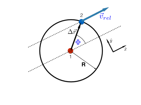
Figure -1259: Schematic picture of two colliding particles in the frame of particle 1, where particle 2 has the relative velocity $\vec{v}_{rel}=\vec{v}_{2}-\vec{v}_{1}$ and particle 1 is at rest. The x-axis is chosen parallel to $\vec{v}_{rel}$ to define the polar angle $\Phi$. Here, particle 2 is receding, i.e. is about to leave the interaction circle of the focal particle because $\Phi\in[-\pi/2,\pi/2]$.

Another consequence of the neglect of triple collisions is the fact that $P_{2}$ can depend on $\vec{r}_{2}$ only through the difference $\Delta\vec{r}=\vec{r}_{2}-\vec{r}$ which allows us to write $\partial_{\vec{r}}=-\partial_{\Delta\vec{r}}$ and $\partial_{\vec{r}_{2}}=\partial_{\Delta\vec{r}}$. The two-dimensional Gauss-theorem for a vector field $\vec{A}$,

$$\int d\vec{r}\,div\vec{A}=\oint\vec{A}\cdot\hat{r}\,ds$$ (24)

allows us to express the integral over the area of the collision circle as an integral over the edge of this circle. Using the relative velocity of particle $2$ in the co-moving frame of the focal particle, $\vec{v}_{rel}=\vec{v}_{2}-\vec{v}=v_{0}(\hat{n}(\theta_{2})-\hat{n}(\theta))$, as new $x$-axis, we define the polar angle $\phi$ as the angle between $\vec{v}_{rel}$ and $\Delta\vec{r}$, see Fig. -1259. Substituting the arc length $ds=R\,d\phi$ and the radial vector $\hat{r}=R({\rm cos}\phi,{\rm sin}\phi)$ we arrive at

$$J^{(coll)}=(N-1)R\,\int_{0}^{2\pi}d\theta_{2}\int_{0}^{2\pi}d\phi\;v_{rel}\,{\rm cos}\phi\,P_{2}$$ (25)

The advantages of this representation are that we only need to specify $P_{2}$ on the edge of the interaction circle and that the number of integrations is reduced by one. It is interesting to note that neither the interaction strength $\Gamma$ nor the interaction kernel ${\rm sin}(\theta_{2}-\theta)$ occur anymore in the collision integral. However, there has to be an implicit dependence on the coupling strength $\Gamma$. Therefore, as a consistence test, let us check the limit $\Gamma\rightarrow 0$ where particles evolve independently of each other and the collision integral is expected to vanish. For a noninteracting system the two-particle density $P_{2}$ factorizes exactly, that is $P_{2}=P_{1}(\vec{r},\theta)\,P_{1}(\vec{r}_{2},\theta_{2})$. Since there is no dependence on the vector connecting both particles, and thus no dependence on $\phi$, the integral over the polar angle gives zero. Thus, as expected, the collision integral vanishes at $\Gamma=0$.

This observation also means that a naive factorization of $P_{2}$ in Eq. (25) similar to the one in the derivation of the Vlasov equation cannot capture the effect of the interactions. This is were the concept of one-sided molecular chaos comes into play, where the factorization is only used when the two particles start their interaction. In Fig. -1259 we see that if the angle $\phi$ is between $\pi/2$ and $3\pi/2$, the two particles reduce their mutual distance from an initial distance $R$, i.e. are approaching. If $\phi$ is between $-\pi/2$ and $+\pi/2$ the distance between them will be increasing, away from the initial value of $R$. In this case we have receding particles. We split the integral over $\phi$ into two domains, one for approaching particles and one for receding particles, and for a periodic integrand we have

$$\int_{0}^{2\pi}d\phi\ldots=\int_{-\pi/2}^{\pi/2}d\phi\ldots+\int_{\pi/2}^{3\pi/2}d\phi\ldots$$ (26)

In the approaching domain, we assume molecular chaos at impact, that is we factorize $P_{2}=P_{1}(\vec{r},\theta)\,P_{1}(\vec{r}_{2},\theta_{2})$ and introduce the new variable $\hat{\phi}=\phi-\pi$, leading to ${\rm cos}\phi=-{\rm cos}\hat{\phi}$ and the same integration boundaries as in the receding domain. Relabeling $\hat{\phi}$ by $\phi$ again, we obtain:

$$J^{(coll)}=(N-1)R\,\int_{0}^{2\pi}d\theta_{2}\,v_{rel}\int_{-\pi/2}^{\pi/2}d\phi\;{\rm cos}\phi\,\big{[}P_{2}|_{rec}-P_{1}(\vec{r},\theta,t)\,P_{1}(\vec{r}_{2},\theta_{2},t)\big{]}\bigg{|}_{\Delta r=R}$$ (27)

In the receding part of the integral, $P_{2}$ cannot be factorized because until this time $t$ (when the two particles are about to leave their encounter) they had continuously interacted over the time period $T_{Dur}$ and thus, are correlated. However, (i) we exactly know how they have interacted during that time, and (ii) we assume that they were uncorrelated at the earlier “entrance” time $t_{0}=t-T_{Dur}$ when they first came in contact with each other. Since we know the positions and angles of the particles when they emerge from their encounter at time $t$ (because this is given by the integration variables in the receding part of the collision integral) , and since the dynamics is deterministic, we can integrate the microscopic evolution equations backwards in time until the entrance time $t_{0}$ where the mutual distance is again at the value $R$. It turns out that this backtracing from the exit time $t$ to time $t_{0}<t$ can be done exactly for the noise-free VM, see Appendix A where the dynamics of two interacting particles is calculated explicitly.

For a fluid with Hamiltonian dynamics, the so-called super position principle kreuzer_81 relates probability densities of particles at different times. It therefore allows the factorization of $P_{2}$ using $P_{1}$ at earlier times, and hence incorporates the aformentioned assumption (ii) in a simple way. However, the superposition principle relies on the fact that the phase space compression factor evans_08 is zero in Hamiltonian systems, which is not the case here. Therefore, in the following chapter we develop a modified superposition principle for the noise-free VM.

III.4 Phase space compression and superposition principle

From the Liouville theory of classical mechanics it is well-known that the infinitesimal volume of phase space does not change along a trajectory and that the total time derivative of the phase space density is zero. However, if the equations of motion are not generated by a Hamiltonian, this is not neccessarily the case. Instead, a phase space compression factor $\Lambda_{N}$ evans_08 determines the total time derivative for a N-particle system,

$${d\over dt}P_{N}=-\Lambda_{N}\,P_{N}$$ (28)

where $\Lambda_{N}$ depends on the phases of the system.

For $N=2$ interacting particles, the total time derivative reads,

$${d\over dt}P_{2}(\vec{r}(t),\theta(t),\vec{z}(t),\beta(t),t)=\bigg{[}\partial_{t}+\dot{\vec{r}}\cdot\partial_{\vec{r}}+\dot{\theta}\,\partial_{\theta}+\dot{\vec{z}}\cdot\partial_{\vec{z}}+\dot{\beta}\,\partial_{\beta}\bigg{]}\,P_{2}$$ (29)

Inserting the microscopic rules of the noise- and field-free VM, Eqs.(1, 2), at close range, gives

$${d\over dt}P_{2}=\bigg{[}\partial_{t}+v_{0}\hat{n}(\theta)\cdot\partial_{\vec{r}}+\Gamma{\rm sin}(\beta-\theta)\,\partial_{\theta}+v_{0}\hat{n}(\beta)\cdot\partial_{\vec{z}}+\Gamma{\rm sin}(\theta-\beta)\,\partial_{\beta}\bigg{]}\,P_{2}$$ (30)

Using the product rule in the differentiations in the second hierarchy equation, Eq. (19), at zero noise and without external field, gives

$$\big{[}\partial_{t}+v_{0}\hat{n}(\theta)\cdot\partial_{\vec{r}}+\Gamma{\rm sin}(\beta-\theta)\,\partial_{\theta}+v_{0}\hat{n}(\beta)\cdot\partial_{\vec{z}}+\Gamma{\rm sin}(\theta-\beta)\,\partial_{\beta}\big{]}\,P_{2}=2\Gamma P_{2}\,{\rm cos}(\beta-\theta)$$ (31)

Terms containing $P_{3}$ vanish exactly because only two particles exist in this case. Replacing the right side of Eq. (30) by Eq.(31) gives

$${d\over dt}P_{2}=2\Gamma\,{\rm cos}(\beta-\theta)\,P_{2}$$ (32)

where we can read off the phase space compression factor for the two-particle VM,

$$\Lambda_{2}=-2\Gamma\,{\rm cos}(\beta-\theta)$$ (33)

Taking time as the only independent variable, Eq. (32) can be integrated from time $t_{0}$ to $t$. Changing variables $\vec{z}=\vec{r}_{2}$, $\beta=\theta_{2}$ one obtains:

$$P_{2}(\vec{r}(t),\theta(t),\vec{r}_{2}(t),\theta_{2}(t),t)=$$

$$P_{2}(\vec{r}(t_{0}),\theta(t_{0}),\vec{r}_{2}(t_{0}),\theta_{2}(t_{0}),t_{0})\;{\rm exp}\Bigg{[}2\Gamma\int_{t_{0}}^{t}d\tilde{t}\,{\rm cos}\{\theta_{2}(\tilde{t})-\theta(\tilde{t})\}\Bigg{]}$$ (34)

This is the superposition principle for the VM. It reduces to the common principle of a classical gas in the limit of vanishing alignment, $\Gamma=0$. Note, that the extended superposition principle depends on the microscopic details of the model. As pointed out in ihle_23a the same result (34) can be obtained when the Liouville-equation of a two-particle system (within interaction range $R$) is solved exactly by the method of characteristics, where the charcteristics are given by the actual trajectories of the particles.

III.5 One-sided molecular chaos and the forbidden zone

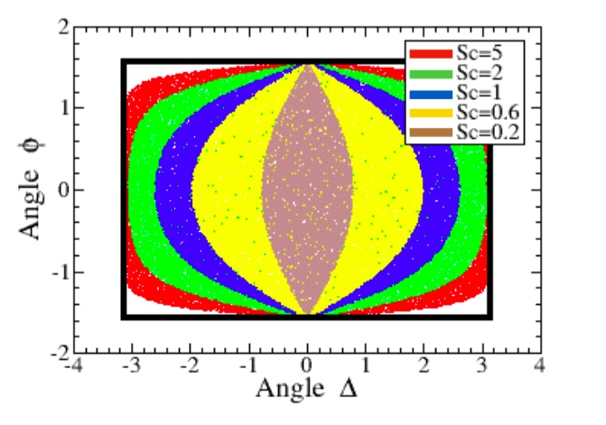
Figure -1258: Forbidden zone in the angular plane of angles $\phi$ and $\Delta=\theta_{2}-\theta$. The black box denotes the original integration domain, $\Delta\in[-\pi,\pi]$, $\phi\in[-\pi/2,\pi/2]$. For $Sc=0.2$, exit states in the inner seed-shaped brown area are forbidden, i.e. do not occur in reality and, thus, have zero probability. For $Sc=0.6$ states in the yellow and brown areas are forbidden, and so on. The size of the forbidden arera increases with anti-alignment strength $Sc$. At large $Sc\gg 1$, only states in the four corners of the original integration area are “allowed”, i.e. contribute to the collision integral.

We are now in position to complete the treatment of one-sided molecular chaos from chapter III.3: The quantity $P_{2}$ of receding particles that end their encounter at time $t$ is expressed as a functional of $P_{1}$ by means of the superposition principle under the assumption that the two particles were statistically independent at the earlier time $t_{0}$, at the start of their encounter,

$$P_{2}(\vec{r}(t),\theta(t),\vec{r}_{2}(t),\theta_{2}(t),t)\approx$$

$$P_{1}(\vec{r}(t_{0}),\theta(t_{0}),t_{0})\;P_{1}(\vec{r}_{2}(t_{0}),\theta_{2}(t_{0}),t_{0})\,{\rm exp}\Bigg{[}2\Gamma\int_{t_{0}}^{t}d\tilde{t}\,{\rm cos}\{\theta_{2}(\tilde{t})-\theta(\tilde{t})\}\Bigg{]}$$ (35)

However, this factorization at an earlier time for receding particles fails for cases where the dynamics of the model does not allow particular two-particle states $(\vec{r}(t),\theta(t),\vec{r}_{2}(t),\theta_{2}(t))$ at all. For $M\rightarrow 0$ these cases do not occur in reality but in the mathematical evaluation of the collision integral, and have to be properly taken into account. As explained further below in the evaluation of Eq. (41), for anti-alignment interactions, that is for $\Gamma<0$, this often occurs for small differences between the two angles at the exit time $t$. In those cases, we simply set $P_{2}(\vec{r}(t),\theta(t),\vec{r}_{2}(t),\theta_{2}(t),t)=0$ in the collision integral. This amounts to a reduction of the integration domain in the collision integral for receding particles at exit time $t$. The removed section of the integration domain will be called forbidden zone and is pictured in Fig. -1258. While there are also quite improbable two-particle states for approaching particles, this is always ignored on the level of a Boltzmann-like description and is subject of further research. Within Boltzmann-like approaches, the incoming particles are always considered as completely independent, something we know since 1970 from the work by Alder and Wainright alder_70 is not true for regular, classical fluids where momentum is conserved during collisions.

The “price” for a Boltzmann-like description, that is, for the simplicity of having an equation for $P_{1}$ alone, is to sacrifice the complete knowledge of the time evolution of the system. Our aim here is to obtain a description that is only valid on length scales of the mean free path $\lambda_{free}$ and on time scales of the mean free time and beyond. The binary collision approximation applied earlier only makes sense if the duration of the encounters $T_{dur}$ is much smaller than $T_{free}$ and consequently, the interaction range $R$ must also be much smaller than $\lambda_{free}$. This means, in a coarse grained description on the scales of $\lambda_{free}$ and $T_{free}$ we can assume $t\approx t_{0}$ and $\vec{r}(t)\approx\vec{r}_{2}(t)\approx\vec{r}(t_{0})\approx\vec{r}_{2}(t_{0})$ in the arguments of $P_{1}$ and $P_{2}$ in Eq. (35). Hoever, the angular changes, for example, $\theta(t)-\theta(t_{0})$ during the collision, as well as the time difference $t-t_{0}$ in the phase space compression integral can be significant and have to be treated in detail. This coarse-graining leads to a simplification of Eq. (35):

$$P_{2}(\vec{r},\theta,\vec{r}_{2},\theta_{2},t)\approx$$

$$P_{1}(\vec{r},\theta_{ent},t)\,P_{1}(\vec{r},\theta_{2,ent},t)\,{\rm exp}\Bigg{[}2\Gamma\int_{t_{0}}^{t}d\tilde{t}\,{\rm cos}\{\theta_{2}(\tilde{t})-\theta(\tilde{t})\}\Bigg{]}$$ (36)

where $\theta_{ent}$ and $\theta_{2,ent}$ are the angles of the two particles at the entrance time $t_{0}$ (when they first started their encounter) that leads to their departure at the later time $t$ with angles $\theta$ and $\theta_{2}$. Thus, these entrance angles are functions of the exit angles $\theta$ and $\theta_{2}$ as well as of the direction of the vector $\Delta\vec{r}$ which connects the particles at the exit time $t$. These dependencies, such as $\theta_{ent}=\theta_{ent}(\theta,\theta_{2},\Delta\vec{r})$ and $T_{Dur}=T_{Dur}(\theta,\theta_{2},\Delta\vec{r})$ are analytically derived in section III.6.3 using the results from Appendix A for the dynamics of two particles. For the noise-free VM, the calculations could be done exactly with the following results:

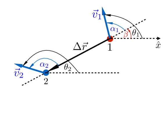
Figure -1257: Schematic picture of particles 1 and 2 with the definition of the connecting vector $\Delta\vec{r}$, and the angles $\alpha_{1}$, $\alpha_{2}$, $\beta$, $\theta_{1}$ and $\theta_{2}$.

In a two-particle interaction, the sum of the angles of the two involved particles $\tilde{c}=\theta_{2}+\theta$ is conserved during the time evolution, see Appendix A. However, the angular difference $\Delta=\theta_{2}-\theta$ changes during the backtracing from $t$ to $\tilde{t}$ with $t_{0}\leq\tilde{t}\leq t$ according to

$${\rm tan}\Big{[}{\Delta(\tilde{t})\over 2}\Big{]}={\rm tan}\Big{[}{\Delta(t)\over 2}\Big{]}\,{\rm exp}\big{[}2\Gamma(t-\tilde{t})\big{]}$$ (37)

For $\Gamma<0$ this means that the difference decreases in the backwards evolution. The distance between the two particles evolves during backwards evolution in the following way,

$$\Delta r(\tilde{t})=\sqrt{R^{2}+4v_{0}^{2}G\Big{(}G+{R\over v_{0}}\,{\rm sin}{c\over 2}\Big{)}}$$ (38)

where $G$ is a time-dependent function,

$$G(t-\tilde{t})={1\over 2\,\Gamma}\Bigg{[}{\rm asinh}\mu-{\rm asinh}\big{\{}\mu\,{\rm exp}(2\Gamma(t-\tilde{t}))\big{\}}\Bigg{]}\,,$$ (39)

with the abbreviation $\mu\equiv{\rm tan}[\Delta/2]$ where $\Delta\equiv\Delta(t)=\alpha_{2}(t)-\alpha_{1}(t)=\theta_{2}-\theta$. The quantity $c$ in Eq. (38) is the sum of the flying directions $\alpha_{1}$ and $\alpha_{2}$ with respect to the connecting vector of the particles, see Fig. -1257, and is taken at the (fixed) exit time $t$, $c\equiv\alpha_{1}(t)+\alpha_{2}(t)$. According to Eq. (39), at the exit time $\tilde{t}=t$, $G$ is equal to zero, and Eq. (38) delivers the required result: $\Delta r(t)=R$. Tracing time backwards with $\tilde{t}<t$ (for particles that fulfill the receding condition), one sees that independent of the sign of the coupling constant $\Gamma$, the particle’s distance becomes initially smaller than $R$, i.e. the particles engage in the alignment interaction. Typically, after a certain time, the distance starts increasing again. At the particular time $\tilde{t}=t_{0}$ when the bracket in Eq. (38) becomes zero, the distance has reached the value $R$ again, which defines the entrance time $t_{0}$,

$$G(t-t_{0})+{R\over v_{0}}\,{\rm sin}{c\over 2}=0$$ (40)

Substituting $G$ from Eq. (39) gives the following expression for the duration $T_{Dur}=t-t_{0}$ of the interaction,

$$T_{Dur}={1\over 2\,\Gamma}\,{\rm ln}\Bigg{\{}{{\rm sinh}\big{[}{\rm asinh}(\mu)+{2\,\Gamma R\over v_{0}}\,{\rm sin}{c\over 2}\big{]}\over\mu}\Bigg{\}}\,.$$ (41)

The angular difference $\Delta(t_{0})$ at the start of an interaction can be determined by inserting the calculated duration of the interaction, Eq. (41), into Eq. (37), resulting into

$${\rm asinh}\Bigg{[}{\rm tan}\bigg{(}{\Delta(t_{0})\over 2}\bigg{)}\Bigg{]}={\rm asinh}\Bigg{[}{\rm tan}\bigg{(}{\Delta(t)\over 2}\bigg{)}\Bigg{]}+{2\,\Gamma R\over v_{0}}\,{\rm sin}{c\over 2}$$ (42)

One sees that, as expected, for $\Gamma=0$ there is no change of the angles, and for negative $\Gamma$ the initial angular difference has a smaller absolute value than at the exit point.

If the argument of the logarithm in Eq. (41) is negative, there is no real solution for the time duration. This indicates that the point $(\vec{r},\theta,\vec{r}_{2},\theta_{2})$ cannot be reached by the dynamics of the system, i.e. amounts to a point in an inaccessible, or forbidden part of the 2-particle phase space. Whenever two particles start an interaction they will never be able to leave their encounter with angles from that part of phase space. This is because a non-zero, negative interaction strength $\Gamma$ ensures that their angular difference can not be too small at the exit point. For positive $\Gamma$ and for receding collisions with $-\pi/2\leq\phi\leq\pi/2$, Eq. (41) always has a real solution for the duration time $T_{Dur}$, hence, there is no forbidden zone. Setting the argument of the logarithm to zero gives us criteria for the forbidden zones. For $\Gamma<0$, a two-particle state is in the forbidden zone if

$$|\mu|\leq{\rm sinh}\bigg{(}2\,Sc\,\bigg{|}{\rm sin}{c\over 2}\bigg{|}\bigg{)}$$ (43)

with $Sc=|\Gamma|R/v_{0}$. Thus, angular differences $|\Delta|$ assumed at the exit point of an interaction that are smaller than the critical value $\Delta_{C}$,

$$\Delta_{C}=2{\rm atan}\bigg{[}{\rm sinh}\bigg{(}2\,Sc\,\bigg{|}{\rm sin}{c\over 2}\bigg{|}\bigg{)}\bigg{]}$$ (44)

cannot occur. Hence, $P_{2}=0$ for this state. Since ${\rm sin}(c/2)$ does also depend on $\Delta$, it is better to substitute it be means of Eq. (208) in the argument of the logarithm in Eq. (41) and to use the addition theorem ${\rm sinh}(a+b)={\rm sinh}(a)\,{\rm cosh}(b)+{\rm cosh}(a)\,{\rm sinh}(b)$ to obtain an alternative condition for the forbidden zone in terms of $\Delta$ and $\phi$ as (note, that we are always assuming that $\phi$ is in the receding interval $[\-\pi/2,\pi/2]$ where ${\rm cos}\phi\geq 0$)

$${\rm sin}{|\Delta|\over 2}<{\rm tanh}(2Sc\,{\rm cos}\phi)$$ (45)

where the critical value $\Delta_{C}$ follows as

$$\Delta_{C}=2\,{\rm asin}({\rm tanh}(2Sc\,{\rm cos}\phi))$$ (46)

The maximum possible critical value is obtained for ${\rm cos}\phi=1$ (or ${\rm sin}(c/2)=1$, according to Eq. (208)) with

$$\Delta_{C,max}=2\,{\rm atan}\bigg{[}{\rm sinh}\bigg{(}2\,Sc\,\bigg{)}\bigg{]}=2\,{\rm asin}({\rm tanh}(2Sc)\,.$$ (47)

For large coupling $Sc\gg 1$, $\Delta_{C,max}$ approaches $\pi$,

$$\Delta_{C,max}\approx\pi-4{\rm e}^{-2\,Sc}$$ (48)

This is the expected result, because it means that whatever the angular difference at the entrance of a collision, at strong coupling particles always depart in almost opposite directions. Thus, exit states where the particle angles do not differ that strongly, cannot occur.

III.6 Boltzmann-like scattering theory for weak anti-alignment, $Sc\ll 1$

III.6.1 Handling of the forbidden zone

For negative $\Gamma$, a forbidden section exists in phase space, see Fig. -1258. This can be handled by an appropriate reduction of the integration domain in the collision integral, which will be discussed here. Condition Eq. (46) can be rewritten as a condition for a critical angle $\phi_{C}$ for a given angular difference $\Delta$ as

$${\rm cos}\,\phi_{C}={1\over 2Sc}{\rm atanh}\Big{[}{\rm sin}{|\Delta|\over 2}\Big{]}$$ (49)

The forbidden zone occurs now for angles $\phi$ with ${\rm cos}\phi>{\rm cos}\phi_{C}$. However, on one hand, for angular difference $\Delta$ that are larger than $\Delta_{max}$ given in Eq. (47), the expression for ${\rm cos}\phi_{C}$ gives a value larger than one. This means, no angles $\phi$ (at fixed $\Delta$) qualify for the definition of the forbidden zone. This simply means that once $|\Delta|$ is sufficiently large, all values of $\phi$ from the relevant interval $-\pi/2\leq\phi\leq\pi/2$ are possible, i.e. lead to nonvanishing values of $P_{2}$. On the other hand, for angular differences $|\Delta|<\Delta_{max}$, the cosine ${\rm cos}\phi_{C}$ is smaller than one and, for fixed $\Delta$ there is now a finite (forbidden) interval $[-\phi_{C},\phi_{C}]$ where $P_{2}=0$. Here, we define $\phi_{C}$ as

$$\phi_{C}={\rm acos}\left\{{\rm Min}\left[1,{1\over 2Sc}{\rm atanh}\left({\rm sin}{|\Delta|\over 2}\right)\right]\right\}$$ (50)

where only nonnegative values of the ${\rm acos}$ function are used.

Expanding Eq.(46) for small $Sc$ gives the critical angular difference $\Delta_{C}$,

$$\Delta_{C}=4Sc\,{\rm cos}\phi\Bigg{[}1-{2\over 3}Sc^{2}\,{\rm cos}^{2}\phi\Bigg{]}+O(Sc^{5})$$ (51)

such that for $|\Delta|\leq\Delta_{C}$ the two-particle probability density $P_{2}$ vanishes for receding particles. In linear order in $Sc$, this gives a simple definition of the forbidden zone in terms of the angle $\phi$ for fixed $\Delta$:

$${\rm cos}\phi\geq{\rm cos}\phi_{C}={|\Delta(t)|\over 4\,Sc}+O(Sc^{2})$$ (52)

If $|\Delta(t)|$ is larger than $4\,Sc$, there is no forbidden zone and all angles of $\phi$ are possible. If $|\Delta(t)|$ is smaller than that, there is a finite interval $[-\phi_{C},\phi_{C}]$ in which $P_{2}$ does vanish. This motivates the following splitting of the integration over $\theta_{2}$ in the collision integral (assuming periodicity of the integrand):

$$\int_{-\pi}^{\pi}d\theta_{2}\ldots=\int_{-4\,Sc+\theta}^{4\,Sc+\theta}d\theta_{2}\ldots+\int_{-\pi+\theta}^{-4\,Sc+\theta}d\theta_{2}\ldots+\int_{4\,Sc+\theta}^{\pi+\theta}d\theta_{2}\ldots$$ (53)

The first integral contains the forbidden zone, meaning that not all angles $\phi$ are allowed in it. In the following two integrals, all angles of $\phi$ are possible. This leads to the final splitting of the two-dimensional collision integral for receding particles:

$$\int_{-\pi}^{\pi}d\theta_{2}\int_{-\pi/2}^{\pi/2}d\phi\ldots=$$

$$\int_{-4\,Sc+\theta}^{4\,Sc+\theta}d\theta_{2}\Bigg{\{}\int_{-\pi/2}^{-\phi_{C}}d\phi\ldots+\int_{\phi_{C}}^{\pi/2}d\phi\ldots\Bigg{\}}$$

$$+\int_{-\pi+\theta}^{-4\,Sc+\theta}d\theta_{2}\int_{-\pi/2}^{\pi/2}d\phi\ldots+\int_{4\,Sc+\theta}^{\pi+\theta}d\theta_{2}\int_{-\pi/2}^{\pi/2}d\phi\ldots$$ (54)

where we have already removed the forbidden part because the integrand is zero there. As long as $Sc$ is not too large, $Sc<\pi/4$, this splitting works, at least formally. Of course, at larger $Sc$ the expression for $\phi_{C}$ is not quantitatively correct anymore and nonlinearities of $O(Sc^{2})$ and higher, according to Eq. (50), need to be taken into account.

III.6.2 The duration of the encounter

Expanding the duration time, Eq. (41), for small $Sc$ gives

$$T_{Dur}={R\over v_{0}\,\mu}{\rm sin}{c\over 2}\Bigg{[}\sqrt{1+\mu^{2}}-{\Gamma R\over v_{0}\mu}{\rm sin}{c\over 2}+{4\Gamma^{2}R^{2}\over 3v_{0}^{2}\mu^{2}}{\rm sin}^{2}{c\over 2}\Bigg{]}$$ (55)

where ${\rm cosh}({\rm asinh}\mu)=\sqrt{1+\mu^{2}}$ was used. For zero coupling, $\Gamma=0$, particles just fly straight through the interaction circle and the duration becomes

$$T_{Dur,0}={R\over v_{0}}{\rm sin}\Big{(}{c\over 2}\Big{)}{\sqrt{1+\mu^{2}}\over\mu}={R\over v_{0}}{{\rm cos}\phi\over|{\rm sin}{\Delta(t)\over 2}|}$$ (56)

where Eqs.(202, 208) were used. Eq. (56) confirms that $T_{Dur,0}$ is always positive for a receding collision where $\pi/2\leq\phi\leq\pi/2$. For small $\Gamma\neq 0$, one has

$$T_{Dur}=T_{Dur,0}-{\rm sgn}(\Gamma)\,Sc{R\over v_{0}}\,\Bigg{(}{{\rm cos}\phi\over{\rm tan}{\Delta(t)\over 2}}\Bigg{)}^{2}+O(Sc^{2})$$ (57)

Anti-alignment, i.e. $\Gamma<0$, leads to a decrease of the angular difference during back-tracing, which makes it harder for the particles to separate from each other. In contrast, for positive $\Gamma$ the angular difference increases in the back-wards time evolution, leading to a faster increase of their distance, and thus to a shorter interaction time. Thus, in first order in $Sc$, for $\Gamma<0$, the duration of the encounter is increased compared to the non-interacting case, as quantified by Eq. (57). At first sight, this result seems to be counter-intuitive as it is well-known that particles stay together longer due to ferromagnetic alignment and shorter if anti-alignment is present. This puzzle is resolved by noting that we do not consider the average duration of all encounters but that we select only receding particles, that is particles that just underwent a binary collision, and analyse the effect of the interaction on the duration of their encounter by backtracing in time. In the former case, one would place the condition of an approaching pair of particles on the evaluation, whereas in the latter case, the condition of a receding pair is used, resulting in qualitatively different outcomes.

III.6.3 The change of the flying angles during the interaction

To properly close the first BBGKY-equation by the extended super position principle (36), explicit relations for the entrance angles, $\theta_{ent}=\theta(t_{0})$ and $\theta_{2,ent}=\theta_{2}(t_{0})$ as functions of the exit angles and the connecting angle $\Phi$ are needed. Because $\theta+\theta_{2}$ stays constant during a two-particle collision, see Appendix A, one has

$$\theta(t_{0}) = {1\over 2}\big{[}\theta(t)+\theta_{2}(t)-\Delta(t_{0})\big{]}$$

$$\theta_{2}(t_{0}) = {1\over 2}\big{[}\theta(t)+\theta_{2}(t)+\Delta(t_{0})\big{]}$$ (58)

Substituting Eq. (208) into (42), the difference of the angles at entrance time $t_{0}$ is obtained as

$$\Delta(t_{0})=2{\rm atan}\Bigg{\{}{\rm sinh}\Bigg{[}{\rm asinh}\Big{[}{\rm tan}\bigg{(}{\Delta(t)\over 2}\bigg{)}\Big{]}+{2\Gamma R\over v_{0}}\,{\rm cos}\phi\;{\rm sgn}\Bigg{(}{\rm sin}{\Delta(t)\over 2}\Bigg{)}\Bigg{]}\Bigg{\}}$$ (59)

For weak coupling $Sc=|\Gamma|R/v_{0}\ll 1$ and sufficiently large initial differences $\Delta(t)$ such that $|\mu|\gg 2\,Sc|\cos{\phi}|$, expression (59) can be expanded in terms of $\epsilon\equiv 2\Gamma R\cos{\phi}\,{\rm sgn}({\rm sin}{\Delta(t)/2})/v_{0}$ as

$$\Delta(t_{0}) = 2\,{\rm atan}\Bigg{[}\mu+\epsilon\sqrt{1+\mu^{2}}+{\epsilon^{2}\over 2}\mu+{\epsilon^{3}\over 6}\sqrt{1+\mu^{2}}+\ldots\Bigg{]}$$ (60)

$$= \Delta(t)+{2\epsilon\over\sqrt{1+\mu^{2}}}-{\epsilon^{2}\mu\over 1+\mu^{2}}+O(Sc^{3})$$

$$= \Delta(t)+2\epsilon\,\left|{\rm cos}{\Delta(t)\over 2}\right|-{\epsilon^{2}\over 2}\,{\rm sin}\Delta(t)+O(Sc^{3})$$

$$= \Delta(t)+2\,{\rm sin}\Delta(t)\Bigg{[}\Gamma T_{Dur,0}-{\Gamma^{2}R^{2}\over v_{0}^{2}}{\rm cos}^{2}\phi\Bigg{]}+O(Sc^{3})$$

where the last equality is only valid for $-\pi\leq\Delta\leq\pi$. Combining Eqs. (58,60) we find for weak coupling:

$$\theta(t_{0}) = \theta(t)-{\rm sin}\Delta(t)\Bigg{[}\Gamma T_{Dur,0}-{\Gamma^{2}R^{2}\over v_{0}^{2}}{\rm cos}^{2}\phi\Bigg{]}+O(Sc^{3})$$ (61)

$$\theta_{2}(t_{0}) = \theta_{2}(t)+{\rm sin}\Delta(t)\Bigg{[}\Gamma T_{Dur,0}-{\Gamma^{2}R^{2}\over v_{0}^{2}}{\rm cos}^{2}\phi\Bigg{]}+O(Sc^{3})$$ (62)

III.6.4 The phase space compression integral

The integral in the extended superposition equation, Eq. (36), which reflects phase space compression, is transformed by means of a trigonometric identity,

$$J_{S}=\int_{t_{0}}^{t}d\tilde{t}\,{\rm cos}\{\theta_{2}(\tilde{t})-\theta(\tilde{t})\}\Bigg{]}=\int_{t_{0}}^{t}d\tilde{t}\,{1-\tilde{\mu}^{2}\over 1+\tilde{\mu}^{2}}$$ (63)

with $\tilde{\mu}\equiv{\rm tan}(\theta_{2}(\tilde{t})-\theta(\tilde{t})/2$. Using Eq.(37), it is rewritten as

$$J_{S}=\int_{t_{0}}^{t}d\tilde{t}\,{1-\mu^{2}{\rm exp}(4\Gamma(t-\tilde{t}))\over 1+\mu^{2}{\rm exp}(4\Gamma(t-\tilde{t}))}\,,$$ (64)

and by means of the transformation $x={\rm exp}(2\Gamma(t-\tilde{t}))$ it is solved exactly as

$$J_{S} = {1\over 2\Gamma}\int_{\mu}^{\mu\,{\rm exp}(2\Gamma(t-t_{0}))}{1-x^{2}\over x(1+x^{2})}\,dx$$

$$= {1\over 2\Gamma}\int_{\mu}^{\mu\,{\rm exp}(2\Gamma(t-t_{0}))}\left({1\over x}-{2x\over 1+x^{2}}\right)\,dx$$

$$= {1\over 2\Gamma}\left[{\rm ln}{\mu\,{\rm exp}(2\Gamma(t-t_{0}))\over 1+\mu^{2}\,{\rm exp}(4\Gamma(t-t_{0}))}-{\rm ln}{\mu\over 1+\mu^{2}}\right]$$

$$= t-t_{0}-{1\over 2\Gamma}{\rm ln}{1+\mu^{2}\,{\rm exp}(4\Gamma(t-t_{0}))\over 1+\mu^{2}}$$

$$= {\rm cos}\Delta(t)\,T_{Dur,0}-Sc\,{\rm sgn}(\Gamma){R\over v_{0}}{\rm cos}^{2}\phi\left[{1\over{\rm tan}^{2}(\Delta/2)}+2{\rm cos}^{2}(\Delta/2)\right]+O(Sc^{2})$$ (66)

Note, that substituting $P_{2}$ as given in Eq. (36) into (27) amounts to a non-local closure of the first BBGKY-equation. This is because in this kinetic equation for $P_{1}$ at angle $\theta$, one inserts a functional of $P_{1}$ at the different angles $\theta_{ent}\neq\theta$ and $\theta_{2,ent}\neq\theta$. In principle, there is also a non-locality in position and time, something we neglected in the Boltzmann-style coarse-graining of (35).

III.6.5 Evaluating the collision integral

Calculation of the approaching part

To evaluate the collision integral in Fourier-space, we introduce the angular Fourier transform of the one-particle probability, $\hat{P}_{n}$,

$$\hat{P}_{n}(\vec{r},t)=\int_{0}^{2\pi}{d\theta\over 2\pi}P_{1}(\vec{r},\theta,t){\rm e}^{-in\theta}$$ (67)

and its inverse

$$P_{1}(\vec{r},\theta,t)=\sum_{n=-\infty}^{\infty}\hat{P}_{n}(\vec{r},t){\rm e}^{in\theta}$$ (68)

Multiplying the collision integral, Eq. (27), by ${\rm e}^{-im\theta}/(2\pi)$ and integrating over $\theta$ gives its Fourier component

$$\hat{J}^{(coll)}_{m}=\hat{J}^{(rec)}_{m}+\hat{J}^{(app)}_{m}$$ (69)

where the contribution from approaching particles follows as

$$\hat{J}^{(app)}_{m}=-(N-1)R\sum_{n_{1},n_{2}}\hat{P}_{n_{1}}\hat{P}_{n_{2}}\,\int_{0}^{2\pi}{d\theta\over 2\pi}\int_{0}^{2\pi}d\theta_{2}\,v_{rel}\,\int_{-\pi/2}^{\pi/2}d\phi\,{\rm cos}\phi\;{\rm e}^{i\theta(n_{1}-m)+in_{2}\theta_{2}}$$ (70)

Inserting $v_{rel}=2v_{0}|{\rm sin}(\Delta/2)|$ from Eq. (207) and performing the integration over $\phi$ gives

$$\hat{J}^{(app)}_{m}=-4(N-1)Rv_{0}\sum_{n_{1},n_{2}}\hat{P}_{n_{1}}\hat{P}_{n_{2}}\,\int_{0}^{2\pi}{d\theta\over 2\pi}{\rm e}^{i\theta(n_{1}-m)}\hat{K}_{m}(\theta)$$ (71)

with the integral $\hat{K}_{m}$,

$$\hat{K}_{m}(\theta)=\int_{0}^{2\pi}d\theta_{2}\,\left|{\rm sin}{\theta_{2}-\theta\over 2}\right|\,{\rm e}^{in_{2}\theta_{2}}$$ (72)

Since the integrand is periodic we can rewrite this integral as

$$\hat{K}_{m}(\theta) = \int_{\theta}^{\pi+\theta}d\theta_{2}\,{\rm sin}{\theta_{2}-\theta\over 2}\,{\rm e}^{in_{2}\theta_{2}}-\int_{-\pi+\theta}^{\theta}d\theta_{2}\,{\rm sin}{\theta_{2}-\theta\over 2}\,{\rm e}^{in_{2}\theta_{2}}$$ (73)

$$= \int_{\theta}^{\pi+\theta}{d\theta_{2}\over 2i}\,\left[{\rm e}^{i(\theta_{2}-\theta)/2}-{\rm e}^{-i(\theta_{2}-\theta)/2}\right]\,{\rm e}^{in_{2}\theta_{2}}$$

$$- \int_{-\pi+\theta}^{\theta}{d\theta_{2}\over 2i}\,\left[{\rm e}^{i(\theta_{2}-\theta)/2}-{\rm e}^{-i(\theta_{2}-\theta)/2}\right]\,{\rm e}^{in_{2}\theta_{2}}$$

$$= {1\over(1/4)-n_{2}^{2}}\,{\rm e}^{in_{2}\theta}$$

This expression is well-defined for all mode numbers $n_{2}$ and is periodic in $\theta$ as expected. Furthermore, for $n_{2}=0$ it is positive and equal to $4$ as can be verified easily by a direct integration of Eq. (72) for $n_{2}=0$. Substituting $\hat{K}_{m}$ from Eq. (73) into (71) and integrating over $\theta$ yields the final result:

$$\hat{J}^{(app)}_{m}=-4(N-1)\,R\,v_{0}\,\sum_{n=-\infty}^{\infty}{\hat{P}_{n}\,\hat{P}_{m-n}\over(1/4)-(m-n)^{2}}$$ (74)

Note, that the largest contribution to the $m$-th mode of $\hat{J}^{(app)}$ comes from the same mode $n=m$ of $\hat{P}_{n}$, and that the contribution of mode products with larger differences $|m-n|>>1$ of the mode numbers decays inversely proportional to the square of that difference. Thus, we expect that a kinetic description using just a few modes should be sufficient.

Calculation of the receding part in first order in $Sc$

The contribution to the collision integral from receding particles, written in Fourier-space, is

$$\hat{J}^{(rec)}_{m}=(N-1)R\sum_{n_{1},n_{2}}\hat{P}_{n_{1}}\hat{P}_{n_{2}}\left(\hat{H}_{1}+\hat{H}_{2}+\hat{H}_{3}\right)$$ (75)

where we used the integral-splitting of Eq. (54) to define

$$\hat{H}_{1}=\int_{0}^{2\pi}{d\theta\over 2\pi}\int_{-4\,Sc+\theta}^{4\,Sc+\theta}d\theta_{2}\,\Bigg{\{}\int_{-\pi/2}^{-\phi_{C}}d\phi\,Q(\theta,\theta_{2},\phi)+\int_{\phi_{C}}^{\pi/2}d\phi\,Q(\theta,\theta_{2},\phi)\Bigg{\}}$$ (76)

$$\hat{H}_{2}=\int_{0}^{2\pi}{d\theta\over 2\pi}\int_{-\pi+\theta}^{-4\,Sc+\theta}d\theta_{2}\,\int_{-\pi/2}^{\pi/2}d\phi\,Q(\theta,\theta_{2},\phi)$$ (77)

$$\hat{H}_{3}=\int_{0}^{2\pi}{d\theta\over 2\pi}\int_{4\,Sc+\theta}^{\pi+\theta}d\theta_{2}\,\int_{-\pi/2}^{\pi/2}d\phi\,Q(\theta,\theta_{2},\phi)$$ (78)

with the kernel

$$Q(\theta,\theta_{2},\phi)=v_{rel}\,{\rm e}^{2\Gamma\,J_{S}}\,{\rm cos}\phi\,{\rm exp}\left[-i\theta m+in_{1}\theta_{entr}+in_{2}\theta_{2,entr}\right]$$ (79)

where $J_{S}$, given in Eq. (66), describes phase space compression, and where $v_{rel}=2v_{0}|{\rm sin}(\Delta/2)|$.

The goal is to first calculate the total collision integral in first order, $O(Sc)$, in the coupling strength $Sc$. Higher order contributions are straightforward but tedius to calculate, and are treated further below. We therefore approximate the kernel $Q$ in the definitions of $\hat{H}_{2}$ and $\hat{H}_{3}$ as

$$Q \approx 2v_{0}\left|{\rm sin}{\Delta\over 2}\right|\,(1+2\Gamma T_{Dur,0}\,{\rm cos}\Delta)\,{\rm cos}\phi\,{\rm e}^{i\theta(n_{1}-m)+in_{2}\theta_{2}}$$ (80)

$$\times\left(1-in_{1}\Gamma T_{Dur,0}\,{\rm sin}\phi\right)\left(1+in_{2}\Gamma T_{Dur,0}\,{\rm sin}\phi\right)$$

$$=2v_{0}\left|{\rm sin}{\Delta\over 2}\right|\,{\rm cos}\phi\,{\rm e}^{i\theta(n_{1}-m)+in_{2}\theta_{2}}$$

$$\times\left(1+\Gamma\,T_{Dur,0}\left[2{\rm cos}\Delta+i(n_{2}-n_{1}){\rm sin}\Delta\right]\right)$$

We cannot use this simple expansion in the integral $\hat{H}_{1}$ because the duration of an encounter $T_{Dur,0}$ diverges for $\Delta\rightarrow 0$, and $|\Gamma\,T_{Dur}|\geq 1$ inside the integral. In this case, an exact treatment of the phase space compresson factor is pursued. Defining $\beta$ as

$$\beta={\rm asinh}\mu+{2\Gamma R\over v_{0}}{\rm sin}{c\over 2}={\rm asinh}\mu+{2\Gamma R\over v_{0}}{\rm sgn}\left({\rm sin}{\Delta/2}\right){\rm cos}\phi$$ (81)

we obtain

$$\mu{\rm e}^{2\Gamma T_{Dur}}={\rm sinh}\beta={\rm tan}{\Delta(t_{0})\over 2}$$ (82)

where the first equality follows from Eq. (41), and the second equality from (42). Inserting Eq. (82) into Eq. (III.6.4), the phase space compression factor is given by

$${\rm e}^{2\Gamma J_{S}}={{\rm sinh}\beta\over 1+{\rm sinh}^{2}\beta}{1+\mu^{2}\over\mu}={{\rm sin}\Delta(t_{0})\over{\rm sin}\Delta(t)}$$ (83)

$$=1+\varepsilon\left[{\sqrt{1+\mu^{2}}\over\mu}-{2\mu\over\sqrt{1+\mu^{2}}}\right]+\varepsilon^{2}{\mu^{2}-5\over 2(1+\mu^{2})}+O(Sc^{3})$$ (84)

$$=1-2\,{\rm sgn}(\Gamma)\,Sc\,{\rm cos}\phi\,{\rm sgn}\left({\rm tan}{\Delta\over 2}\right)\,\left\{2{\rm sin}{\Delta\over 2}-{1\over{\rm sin}{\Delta\over 2}}\right\}$$ (85)

$$+2\,Sc^{2}\,{\rm cos}^{2}\phi{\mu^{2}-5\over 1+\mu^{2}}+O(Sc^{3})$$ (86)

with $\varepsilon\equiv 2\,{\rm sgn}(\Gamma)\,Sc\,{\rm sgn}\left({\rm sin}{\Delta\over 2}\right)\,{\rm cos}\phi$. The integral $\hat{H}_{1}$ takes the following form,

$$\hat{H}_{1}=2v_{0}\int_{0}^{2\pi}{d\theta\over 2\pi}\int_{-4\,Sc+\theta}^{4\,Sc+\theta}d\theta_{2}\,\int_{\Omega}d\phi\,{\rm cos}\phi\,\left|{\rm sin}{\Delta\over 2}\right|{{\rm sinh}\beta\over 1+{\rm sinh}^{2}\beta}{1+\mu^{2}\over\mu}{\rm e}^{iS}$$ (87)

where $\Omega$ is the domain specified in Eq. (76) for the integration over $\phi$, and $S(\theta,\theta_{2},\phi)$ is some phase. Transforming the $\theta_{0}$-integral to the new variable $x=\Delta/(4Sc)=(\theta_{2}-\theta)/(4Sc)$ one has

$$\hat{H}_{1}=8Sc\,v_{0}\int_{0}^{2\pi}{d\theta\over 2\pi}\int_{-1}^{1}dx\,\int_{\Omega}d\phi\,{\rm cos}\phi\,\left|{\rm sin}(2Sc\,x)\right|{{\rm sinh}(2Sc\tilde{\beta})\over 1+{\rm sinh}^{2}(2Sc\,\tilde{\beta})}{1+{\rm tan}^{2}(2Sc\,x)\over{\rm tan}(2Sc\,x)}{\rm e}^{iS}$$ (88)

with $\tilde{\beta}={\rm asinh}[{\rm tan}(2Sc\,x)]/(2Sc)+{\rm sgn}(\Gamma)\,{\rm sgn}(x)\,{\rm cos}\phi$. Since $x$ is of order one, the ${\rm sinh}$, ${\rm sin}$,${\rm tan}$ and ${\rm atan}$ functions can be expanded for small $Sc$ with the result

$$\hat{H}_{1}=16\,Sc^{2}\,v_{0}\int_{0}^{2\pi}{d\theta\over 2\pi}\int_{-1}^{1}dx\,\int_{\Omega}d\phi\,{\rm cos}\phi\,{\rm sgn}(x)\,(x+{\rm sgn}(\Gamma)\,{\rm sgn}(x)\,{\rm cos}\phi)\,{\rm e}^{iS}+O(Sc^{3})$$ (89)

Thus, $\hat{H}_{1}$ is of order $O(Sc^{2})$ and will be neglected in this first oder approach. Inserting the approximated kernel $Q$ from Eq. (80) into the expressions for $\hat{H}_{2}$ and $\hat{H}_{3}$ and integrating over $\phi$ gives

$$\hat{H}_{j}=\int_{0}^{2\pi}{d\theta\over 2\pi}\,{\rm e}^{i\theta(n_{1}-m)}\left\{4v_{0}B_{j1}+\Gamma R\pi\left[2B_{j2}+i(n_{2}-n_{1})B_{j3}\right]\right\}$$ (90)

for $j=2,3$ and the auxiliary integrals

$$B_{21} = -\int_{-\pi+\theta}^{-4Sc+\theta}d\theta_{2}\,{\rm sin}{\theta_{2}-\theta\over 2}\,{\rm e}^{in_{2}\theta_{2}}$$

$$B_{22} = \int_{-\pi+\theta}^{-4Sc+\theta}d\theta_{2}\,{\rm cos}(\theta_{2}-\theta)\,{\rm e}^{in_{2}\theta_{2}}$$

$$B_{23} = \int_{-\pi+\theta}^{-4Sc+\theta}d\theta_{2}\,{\rm sin}(\theta_{2}-\theta)\,{\rm e}^{in_{2}\theta_{2}}$$

$$B_{31} = \int_{4Sc+\theta}^{\pi+\theta}d\theta_{2}\,{\rm sin}{\theta_{2}-\theta\over 2}{\rm e}^{in_{2}\theta_{2}}$$

$$B_{32} = \int_{4Sc+\theta}^{\pi+\theta}d\theta_{2}\,{\rm cos}(\theta_{2}-\theta)\,{\rm e}^{in_{2}\theta_{2}}$$

$$B_{33} = \int_{4Sc+\theta}^{\pi+\theta}d\theta_{2}\,{\rm sin}(\theta_{2}-\theta)\,{\rm e}^{in_{2}\theta_{2}}$$ (91)

One finds,

$$B_{31}={1\over(1/2)-2n_{2}^{2}}{\rm e}^{in_{2}\theta}\left[2n_{2}i(-1)^{n_{2}}+(1-4Sc\,i\,n_{2}){\rm e}^{4Sc\,i\,n_{2}}\right]+O(Sc^{2})$$ (92)

and the exact relation $B_{21}(n_{2})={\rm e}^{2in_{2}\theta}\,B_{31}(-n_{2})$. Thus, the sum is

$$B_{31}+B_{21}={1\over(1/4)-n_{2}^{2}}{\rm e}^{in_{2}\theta}\left[{\rm cos}(4Sc\,n_{2})+4\,Sc\,n_{2}\,{\rm sin}((4Sc\,n_{2})\right]+O(Sc^{2})$$ (93)

This sum has the expected limit for $Sc\rightarrow 0$ but no contribution in $O(Sc)$:

$$B_{31}+B_{21}=\hat{K}_{M}(\theta)+O(Sc^{2}).$$ (94)

Since we only need the sum of $\hat{H}_{2}$ and $\hat{H}_{3}$ in linear order in $Sc$, it suffices to evaluate the following sums

$$\left.B_{22}+B_{32}\right|_{Sc=0}=$$

$$\int_{-\pi+\theta}^{\pi+\theta}{\rm cos}(\theta_{2}-\theta)\,{\rm e}^{in_{2}\theta_{2}}\,d\theta_{2}=\pi{\rm e}^{in_{2}\theta}\left[\delta_{n_{2},-1}+\delta_{n_{2},1}\right]$$ (95)

$$\left.B_{23}+B_{33}\right|_{Sc=0}=$$

$$\int_{-\pi+\theta}^{\pi+\theta}{\rm sin}(\theta_{2}-\theta)\,{\rm e}^{in_{2}\theta_{2}}\,d\theta_{2}=-i\,\pi{\rm e}^{in_{2}\theta}\left[\delta_{n_{2},-1}-\delta_{n_{2},1}\right]$$ (96)

Performing the sum

$$\hat{H}_{1}+\hat{H}_{2}+\hat{H}_{3}=\delta_{m,n_{1}+n_{2}}\left\{\Gamma R\pi^{2}\left[(1-n_{1})\delta_{n_{2},-1}+(1+n_{1})\delta_{n_{2},1}\right]+4v_{0}{1\over(1/4)-n_{2}^{2}}\right\}$$ (97)

and inserting into Eq. (75) gives the collision contribution from the receding particles as

$$J^{(rec)}_{m}=4v_{0}(N-1)R\sum_{n}{\hat{P}_{n}\hat{P}_{m-n}\over(1/4)-(m-n)^{2}}+(N-1)\Gamma R^{2}\pi^{2}m\left[\hat{P}_{m-1}\hat{P}_{1}-\hat{P}_{m+1}\hat{P}_{-1}\right]$$ (98)

Adding both contributions from receding and approaching particles leads to the final result for the collision integral in Fourier space at order $O(Sc)$,

$$J^{(coll)}_{m}=J^{(rec)}_{m}+J^{(app)}_{m}=(N-1)\Gamma R^{2}\pi^{2}m\left[\hat{P}_{m-1}\hat{P}_{1}-\hat{P}_{m+1}\hat{P}_{-1}\right]+O(Sc^{2})$$ (99)

Remembering that $P=f/N$ and $\hat{P}_{n}/N=\hat{f}_{n}/N$, one realizes that the collision integral for large particle number, $N>>1$, and in linear order in $Sc$, is identical to the one we had obtained by the much simpler mean-field approximation in chapter II. This is rather surprising as we explicitly treated the (correlated) alignment interactions over the duration of the collision encounter. In the following section we will see that the difference between the simple factorization approximation and the one-sided molecular chaos assumption shows up for the first time in second order in the coupling strength $Sc$. This is partly due to the fact that the effect of the “forbidden zone” did not enter the calculations in linear order in $Sc$.

Calculation of the receding part in second order in $Sc$

We find

$$\hat{H}_{2}+\hat{H}_{3}=2v_{0}\delta_{n_{1}+n_{2},m}\left\{2B_{1}(\pi)-{\pi\over 2}\,Sc\,\left[i\Delta n\,B_{3}(\pi)+2B_{2}(\pi)\right]\right.$$

$$+\left.{4\over 3}\,Sc^{2}\left[-{(\Delta n)^{2}\over 2}A_{1}(\pi)+2I(\pi)+2i\,\Delta n\,A_{2}(\pi)-i\,\Delta n\,A_{3}(\pi)\right]\right.$$

$$\left.-2B_{1}(4\,Sc)+{\pi\over 2}Sc\left[i\,\Delta n\,B_{3}(4Sc)+2B_{2}(4Sc)\right]+O(Sc^{3})\right\}$$ (100)

with $\Delta n\equiv n_{2}-n_{1}$. The quantities $A_{i}$ and $B_{i}$ are angular integrals which are defined and calculated in Appendix C. The auxiliary quantity $I$ in Eq. (100) can be expressed in terms of integrals $A_{i}$ as

$$I(\pi)=\int_{-\pi}^{\pi}{\mu^{2}(x)-5\over 1+\mu^{2}(x)}\,\left|{\rm sin}{x\over 2}\right|\,{\rm e}^{in_{2}x}\,dx=-A_{1}(\pi)-A_{4}(\pi)$$ (101)

with $\mu(x)={\rm tan}(x/2)$. The part $\hat{H}_{1}$ is of second order in Sc, and one obtains

$$\hat{H}_{1}=16\,Sc^{2}\,v_{0}\delta_{n_{1}+n_{2},m}\,J+O(Sc^{3})$$ (102)

where $J$ is the following double integral:

$$J=\int_{-1}^{1}\,dx\left\{\int_{-\pi/2}^{-\phi_{c}}\,d\phi\,(|x|-{\rm cos}\phi){\rm cos}\phi+\int_{\phi_{c}}^{\pi/2}\,d\phi\,(|x|-{\rm cos}\phi){\rm cos}\phi\right\}$$ (103)

which can be written as $J=J_{0}-J_{1}$ with

$$J_{0} = \int_{-1}^{1}\,dx\,\int_{-\pi/2}^{\pi/2}\,d\phi(|x|-{\rm cos}\phi){\rm cos}\phi=2-\pi$$ (104)

$$J_{1} = \int_{-1}^{1}\,dx\,\int_{-\phi_{c}}^{\phi_{c}}\,d\phi(|x|-{\rm cos}\phi){\rm cos}\phi$$ (105)

Since at this order in $Sc$ we have ${\rm cos}\phi_{c}\approx|x|$, the integral can be solved by the transformation $x={\rm cos}y$, and one finds $J_{1}=-4/3$. Thus, finally we obtain

$$\hat{H}_{1}=16\,Sc^{2}\,v_{0}\delta_{n_{1}+n_{2},m}\left[{10\over 3}-\pi\right]$$ (106)

Adding $\hat{H}_{1}$ to $\hat{H}_{2}+\hat{H}_{3}$, inserting in Eq. (75) and collecting only terms of order $Sc^{2}$ one finds the following addition to the collision integral $\hat{J}_{m}^{(coll)}$ that goes beyond naive mean-field theory:

$$(N-1)Rv_{0}\,Sc^{2}\,\sum_{n_{1},n_{2}}\hat{P}_{n_{1}}\hat{P}_{n_{2}}\delta_{n_{1}+n_{2},m}\left\{{8\over 3}\left[{1\over n_{2}^{2}-{1\over 4}}\left(1-3\Delta n\,n_{2}+{1\over 2}\Delta n^{2}\right)\right.\right.$$

$$\left.\left.+{1\over n_{2}^{2}-{9\over 4}}\left(9-5\Delta n\,n_{2}+{3\over 2}\Delta n^{2}\right)\right]\right\}$$ (107)

This new contribution can be written by means of a coupling matrix $g_{m,n}$,

$$\hat{J}_{m}^{(new)}=(N-1)Rv_{0}\,Sc^{2}\,\sum_{n=-\infty}^{\infty}\hat{P}_{n}\hat{P}_{m-n}g_{m,n}$$ (108)

with

$$g_{m,n}={8\over 3}m\left[{{3\over 2}m-n\over(m-n)^{2}-{1\over 4}}+{n+{1\over 2}m\over(m-n)^{2}-{9\over 4}}\right]$$ (109)

The coupling matrix has a rather intricate form and it is useful to establish symmetry requirements to check its consistency. Because of mass conservation, the mode $\hat{f}_{0}=\rho_{0}/(2\pi)$ should never change in a homogeneous system. As a consequence, the collision integral should be zero for $m=0$. This amounts to a non-trivial cancellation of terms in the contributions $\hat{H}_{j}$, $j=1,2,3$. Thus, the coupling matrix $g_{m,n}$ should have the property $g_{0,n}=0$ for all $n$. The distribution $f$ is a real function and therefore its complex Fourier coefficients obey the following relation: $\hat{f}_{-k}=\hat{f}_{k}^{*}$. Considering only real Fourier coefficients (which amounts to solutions that are symmetric with respect to the x-axis) one then expects the following symmetry relation for the coupling matrix

$$g_{-m,-n}=g_{m,n}$$ (110)

The matrix $g_{m,n}$ in Eq. (109) possesses both of the required properties. The validity of the expression for the coupling matrix is further supported numerically in agent-based simulations in chapter V, where the temporal relaxation of the Fouriermodes $\hat{f}$ is measured and compared to the theoretical predictions of the one-sided molecular chaos approximation.

III.7 Self-diffusion and velocity autocorrelation: Boltzmann-Lorentz theory

In general, a Boltzmann equation describes the advection and binary collisions of particles in terms of their probability density $f$. Therefore it contains information about how the particle velocities change during collisions, and thus about the velocity autocorrelation function (vaf). Since one-sided molecular chaos is assumed in the derivation of the Boltzmann equation, particles are expected to “forget” previous encounters before an interaction starts with a new partner. This means, subsequent collision events are uncorrelated and the vaf should decay exponentionally, at least for time scales larger than $R/v_{0}$ and in situations where the Boltzmann-like equation is expected to be asumptotically exact, i.e. for $M\rightarrow 0$ and $Sc\rightarrow 0$. A similar assumption was made for regular fluids before the numerical discovery of long-time tails in 1970 alder_70 , where it was oberved that the vaf showed a power law decay $\sim t^{-d/2}$ at long times. Here, $d$ denotes the spatial dimension. It was shown that these tails are a consequence of the back-flow effect which relies on momentum-conservation dorfman_70 ; ernst_70 ; kawasaki_71 ; zwanzig_book . However, momentum-conservation does not hold in the “artificial fluid” of self-propelled particles considered here and other sources of such tails seem to be absent in this system of point particles at low densities $M\ll 1$, FOOTNOTE3 . Hence, long-time tails are not plausible in the vaf of the current system; a purely exponential decay of the vaf is expected,

$$C(t)=\langle\vec{v}(0)^{2}\rangle\,{\rm e}^{-t/\tau_{C}}\,,$$ (111)

at least for times much larger than the duraction of a particle collision, $T_{dur}$. According to the Green-Kubo relation,

$$D={1\over d}\int_{0}^{\infty}\langle\vec{v}(t)\cdot\vec{v}(0)\rangle\,dt$$ (112)

which is valid in the stationary state of any fluid, the self-diffusion coefficient $D$ is given by the time integral over the vaf. Relying on the exponential behavior of the vaf, we can easily deduct its correlation time $\tau_{C}$ from the self-diffusion coefficient as

$$\tau_{C}={2D\over v_{0}^{2}}$$ (113)

Therefore, in order to find $\tau_{C}$ it suffices to calculate $D$. This can be done by the so-called Boltzmann-Lorentz theory, see for example hauge_70 and its applications to granular gases brey_99 ; garzo_03 . The main idea is to suppose that several particles are tagged but otherwise all particles are mechanically equivalent. Then, the system is formally considered as a binary system where a population of tagged particles is immersed in a sea of untagged background particles. For our purposes, we tag only one particle, in particular particle $i=1$, and introduce the tagged particle density $h$ as the ensemble average of the corresponding one-particle phase space density,

$$h(\vec{r},\theta)\equiv\langle\delta(\vec{r}-\vec{r}_{1}(t))\,\delta(\theta-\theta_{1}(t))\rangle$$ (114)

The density of the remaining particles is given by

$$\tilde{f}(\vec{r},\theta)\equiv\Big{\langle}\sum_{j=2}^{N}\delta(\vec{r}-\vec{r}_{j}(t))\,\delta(\theta-\theta_{j}(t)\Big{\rangle}$$ (115)

In the thermodynamic limit (td) $N\rightarrow\infty$, it does not matter whether one particle is omitted in the summation of Eq. (115) or not, and $\tilde{f}$ agrees with the function $f$ defined previously, $f=NP_{1}$. In abstract notation, the collision term of the nonlinear Boltzmann equation is given as a functional of $f$ by $J[f,f]$. Here, the first argument in $J$ denotes the function whose evolution is considered; for example $J[f,h]$ would occur in an equation for the density $f$ and describes scatterings of particles from the f-population on members of the h-population. Hence, in general $J[f,h]\neq J[h,f]$. The evolution equation for the tagged particle density contains a collision term of the same functional form $J[h,f]$ because it describes the collision of particle 1 with the other mechanically identical particles. An additional term of type $J[h,h]$ would reflect collisons among tagged particles, which are impossible with only one tagged particle. In the case of a few tagged particles $N_{S}$, these collisions are negligible as their density $N_{S}/V$ goes to zero in the thermodynamic limit $V\rightarrow\infty$ with $N/V=const$. This also means that the collision term in the evolution equation for $h$ – a particular example of the Boltzmann-Lorentz equation – is linear in $h$. In the td-limit, the evolution equation for $\tilde{f}\approx f$ is decoupled from the tagged density $h$, because the collision term $J[\tilde{f},h]$ is smaller than $J[\tilde{f},\tilde{f}]$ by a factor of N.

As explained above, the collision term $J[h,f]$ of the Boltzmann-Lorentz equation and its Fourier-transformed version does not have to be rederived, it follows directly from Eq. (99) and (108) by formally replacing $\hat{f}_{k}$ by $\hat{h}_{k}$ at the appropriate position. Then, the Boltzmann-Lorentz equation for the angular Fourier components of the tagged particle density becomes:

$$\partial_{t}\hat{h}_{m}+{v_{0}\over 2}\left[\nabla^{*}\hat{h}_{m-1}+\nabla\hat{h}_{m+1}\right]$$

$$=\Gamma R^{2}\pi^{2}m\left[\hat{h}_{m-1}\hat{f}_{1}-\hat{h}_{m+1}\hat{f}_{-1}\right]+Rv_{0}(Sc)^{2}\sum_{n=-\infty}^{\infty}\hat{h}_{n}\hat{f}_{m-n}\,g_{m,n}$$ (116)

where the coefficients $g_{m,n}$ are given in Eq. (109), and the terms of order $O(Sc^{0})$ follow from the hierarchy of the Vlasov-like approach, Eq. (14). The first three members of the hierarchy (116) read

$$\partial_{t}\hat{h}_{0}+{v_{0}\over 2}\left[\nabla^{*}\hat{h}_{-1}+\nabla\hat{h}_{1}\right] = 0$$

$$\partial_{t}\hat{h}_{1}+{v_{0}\over 2}\left[\nabla^{*}\hat{h}_{0}+\nabla\hat{h}_{2}\right] = -A\,\pi\Gamma\left[\hat{h}_{2}\hat{f}_{-1}-\hat{h}_{0}\hat{f}_{1}\right]$$

$$+ Rv_{0}\,Sc^{2}\left[\hat{h}_{0}\hat{f}_{1}g_{1,0}+\hat{h}_{1}\hat{f}_{0}g_{1,1}+\hat{h}_{2}\hat{f}_{-1}g_{1,-1}+\ldots\right]$$

$$\partial_{t}\hat{h}_{2}+{v_{0}\over 2}\left[\nabla^{*}\hat{h}_{1}+\nabla\hat{h}_{3}\right] = -2A\,\pi\Gamma\left[\hat{h}_{3}\hat{f}_{-1}-\hat{h}_{1}\hat{f}_{1}\right]$$

$$+ Rv_{0}\,Sc^{2}\left[\hat{h}_{0}\hat{f}_{2}g_{2,0}+\hat{h}_{1}\hat{f}_{1}g_{2,1}+\hat{h}_{2}\hat{f}_{0}g_{2,2}+\ldots\right]$$ (117)

where $\nabla$ and $\nabla^{*}$ are the complex nabla operator and its conjugate, respectively, see Eq. (13).

Assuming a disordered and homogeneous background, all modes of $\hat{f}_{n}$ vanish, except the $n=0$ mode:

$$\hat{f}_{n}=\delta_{n,0}{\rho_{0}\over 2\pi}$$ (118)

where $\rho_{0}$ is the average total particle density. Then, the hierarchy, Eq. (117), simplifies significantly. In particular, all terms related to the Vlasov-part of the collision integral vanish and only terms proportional to $Sc^{2}$ remain. To obtain a diffusion equation for the mode $\hat{h}_{0}$ which is proportional to the density of the tagged particle $\rho_{S}$, we perform a Chapman-Enskog expansion chapman_52 ; hirschfelder_54 ; mcquarrie_76 ; ihle_16 and introduce a small ordering parameter $\epsilon$ which is set to one at the end of the expansion. The spatial gradients are scaled as $\nabla\rightarrow\epsilon\nabla$ and the Fourier-modes are assumed to scale as $\hat{h}_{n}\sim\epsilon^{|n|}$ which can be verified a posteriori. In addition, we introduce the usual multiple time scale expansion of the time derivative,

$$\partial_{t}=\epsilon\partial_{t_{0}}+\epsilon^{2}\partial_{t_{1}}+\ldots$$ (119)

Inserting these expressions into Eq. (117) and collecting terms of the same order, one obtains in linear order, $O(\epsilon)$, $\partial_{t_{1}}\hat{h}_{0}=0$, and

$$\hat{h}_{1}={\nabla^{*}\hat{h}_{0}\over 2R\,Sc^{2}\,\hat{f}_{0}\,g_{1,1}}$$ (120)

meaning that at this order, $\hat{h}_{1}$ is enslaved to the density mode $\hat{h}_{0}$. In second order, $O(\epsilon^{2})$, one finds $\partial_{t_{0}}\hat{h}_{1}=0$, and

$$\partial_{t_{1}}\hat{h}_{0}=-{v\over 2}\left[\nabla^{*}\hat{h}_{-1}+\nabla\hat{h}_{1}\right]$$ (121)

Inserting Eq. (120) in (121), subtituting $g_{1,1}$ from Eq. (109), a diffusion equation is obtained,

$$\partial_{t}\hat{h}_{0} = D\,\Delta\hat{h}_{0}$$ (122)

$$D = {9\pi^{2}Rv_{0}\over 64M\,Sc^{2}}={9\pi^{2}\over 64}{v_{0}^{3}\over R\Gamma^{2}M}$$ (123)

where $\hat{h}_{-1}=\hat{h}_{1}^{*}$, $\nabla\nabla^{*}=\partial_{x}^{2}+\partial_{y}^{2}\equiv\Delta$ and $M=\pi R^{2}\rho_{0}=2\pi^{2}R^{2}\hat{f}_{0}$ from Eq. (118) was used, and $\epsilon$ was set to one. The relaxation time $\tau_{C}$ of the velocity autocorrelation follows from the diffusion coefficient $D$ in Eqs. (113) and (123) as

$$\tau_{C}={9\pi^{2}\over 32}{v_{0}\over R\Gamma^{2}M}$$ (124)

In Ref. ihle_23a it is shown how the exponentially decaying vaf follows directly from Boltzmann-Lorentz theory without the need for Chapman-Enskog expansions and Green-Kubo formulas, leading to the same result for $\tau_{C}$, Eq. (124), and supporting the arguments at the beginning of this chapter.

It is also interesting to note that there is a qualitative difference between the Vlasov-like approximation, where the N-particle probability density is simply factorized and the one-sided molecular chaos (OMC) assumption which takes two-particle correlations within the duration of binary encounters into account: Only the OMC approach can explain the finite relaxation time observed in simulations. The Vlasov-approach, which can formally be considered by setting $Sc=0$ or $\Gamma=0$ in Eqs. (123, 124), incorrectly predicts no relaxation at all, i.e. $\tau_{C}\rightarrow\infty$ which is equivalent to an infinite diffusion coefficient. In VM models with explicit noise terms, the difference between the two approximations is not as drastic, because the noise terms lead to a finite relaxation time, even within the Vlasov-like approach. However, the OMC approximation with external noise that is large enough to significantly modify the particle trajectories during the collision time $\sim R/v_{0}$, is complicated to evaluate and will be left for the future.

The predicted diffusion coefficient, Eq. (123), scales as $\sim 1/M$, i.e. goes to infinity for vanishing density. This is expected since at low $M$, a particle very rarely encounters another one, and thus moves ballistically for very long times. Eq. (123) also predicts scaling with the coupling constant as $D\sim Sc^{-2}$. This is plausible as a vanishing coupling leads to ballistic flights, which corresponds to an infinite diffusion coefficient. Detailed comparisons of the predicted behavior of the diffusion coefficient with agent-based simulations are presented in chapter V and show excellent agreement at small density and small coupling strength.

IV Deriving an effective Langevin-equation

IV.1 Brownian motion of mobile rotators

The random motion of small particles such as pollen grains immersed in a fluid is known as Brownian motion. Einstein’s explanation of its nature can be regarded as the beginning of stochastic modelling of natural phenomena einstein_05 . A simple, approximate way to treat the dynamics of the embedded particle is to model the kicks of the surrounding fluid molecules by a random force in Newton’s equation of motion, something we know now under the name of Langevin equation. The amount of simplification in this description is tremendous since there is no need to describe the details of the interactions among the surrounding molecules or between the molecules and the Brownian particle. All the information about this many-body system is encoded in a friction term and the correlations of the noise, i.e. the random force. In this historic example, these correlations are simple, and the strength of the noise follows from a fluctuation-dissipation relation. In more exotic cases, such as systems of self-driven particles with alignment interactions, it is not a priori clear whether a description by an effective Langevin-equation always makes sense and how to determine the properties of the noise.

There is a few examples on how to analytically derive the properties of the noise by explicitly integrating over the irrelevant degrees of freedom. One of them is due to R.J. Rubin rubin_60 who considered a harmonic lattice in which one particle – the Brownian particle – is much heavier than the rest FOOTNOTE2 . For other, similar systems, see Ref. zwanzig_book . In a more recent example by van Meegen and Lindner vanmeegen_18 , a set of immobile rotators with fixed but randomly chosen frequencies and coupling constants were considered. Using a path integral formalism to average over the frozen disorder, it was shown how to derive the Langevin equation for the angular change $\dot{\theta}$ of a focal rotator and how to obtain the properties of the emerging dynamical noise in this equation.

In this chapter, we will pursue the main general idea of regular Brownian motion and assume that the effects of the surrounding particles on a focal particle can be modeled by a typically colored but Gaussian noise term $\xi$, leading to an effective, one-particle Langevin-equation for the angular change,

$$\dot{\theta}(t)=\xi(t)$$ (125)

The major difference to Refs. rubin_60 ; vanmeegen_18 is that our “rotators” are moving and have no fixed set of interaction partners: the interactions in the VM take place on a time-varying network holme_15 whose links depend on the outcome of the interactions.

We assume here that the correlations of the dynamical noise $\xi=\xi_{i}$ for a given particle $i$ with the one of a different particle $j$, are negligible compared to the correlations of the noise of the same particle, that is $|\langle\xi_{i}(t)\,\xi_{j}(t^{\prime})\rangle|\ll|\langle\xi_{i}(t)\,\xi_{i}(t^{\prime})\rangle|$ for $i\neq j$.

In the following sections, we will show how the kinetic theory with one-sided molecular chaos from chapter III can be utilized to calculate the properties of the noise $\xi$ with high precision in the limit of low density. Using a random-telegraph assumption, we also show how the noise can be determined in the opposite limit of large density.

IV.2 Noise calculation for low particle density

The velocity autocorrelation function (vaf) for particles of constant speed $v_{0}$ can be written as

$$C(\tau)\equiv\langle\vec{v}(t+\tau)\cdot\vec{v}(t)\rangle=v_{0}^{2}\langle{\rm cos}(\Delta\theta)\rangle={v_{0}^{2}\over 2}\Big{[}\Big{\langle}{\rm e}^{i\Delta\theta}\Big{\rangle}+\Big{\langle}{\rm e}^{-i\Delta\theta}\Big{\rangle}\Big{]}$$ (126)

with

$$\Delta\theta\equiv\theta(t+\tau)-\theta(t)=\int_{t}^{t+\tau}dt^{\prime}\,\dot{\theta}(t^{\prime})$$ (127)

According to the assumed effective Langevin-equation, Eq. (125), the angular difference in Eq. (127) can be expressed as the integral over the assumed Gaussian noise $\xi$, $\Delta\theta=\int_{t}^{t+\tau}dt^{\prime}\xi(t^{\prime})$. Thus, $\Delta\theta$ would also be a Gaussian noise. For this kind of noise, the average of the exponentials in Eq. (126) can be expressed as

$$\Big{\langle}{\rm e}^{\pm i\Delta\theta}\Big{\rangle}={\rm exp}\left[-{\langle(\Delta\theta)^{2}\rangle\over 2}\right]$$ (128)

where one has

$$\langle(\Delta\theta)^{2}\rangle=\int_{t}^{t+\tau}dt^{\prime}\int_{t}^{t+\tau}dt^{\prime\prime}\langle\xi(t^{\prime})\xi(t^{\prime\prime})\rangle$$ (129)

and

$$C(\tau)=v_{0}^{2}{\rm exp}\left[-{\langle(\Delta\theta)^{2}\rangle\over 2}\right]\,.$$ (130)

Inserting the simplest kind of noise correlations,

$$\langle\xi(t)\xi(\tilde{t}\rangle=\sigma^{2}\delta(t-\tilde{t})$$ (131)

into Eq. (129) gives

$$\langle(\Delta\theta)^{2}\rangle=\tau\sigma^{2}$$ (132)

Plugging this result into (130) leads to an exponential decay of the vaf:

$$C(\tau)=v_{0}^{2}\,{\rm exp}\left(-{\sigma^{2}\tau\over 2}\right)$$ (133)

i.e. exactly what is predicted by kinetic theory for times larger than $R/v_{0}$ and verified in agent-based simulations at low density $M\ll 1$ and small coupling strength $Sc\ll 1$. Moreover, comparing Eq. (133) with (111) gives an explicit expression for the noise strength of the effective Langevin equation for the angle of a particle:

$$\sigma^{2}={2\over\tau_{C}}={64R\Gamma^{2}M\over 9\pi^{2}v_{0}}$$ (134)

where expression (124) from kinetic theory for $\tau_{C}$ was used. One sees that the effective noise increases with increasing density and coupling strength. This is plausible, since increasing these parameters leads to a stronger scattering of a particle on others which is reflected in a stronger noise. The decrease of the noise with increasing particle velocity also makes sense since the mean free path of a particle increases with velocity.

In summary, by means of a quantitative kinetic theory we were able to construct an effective Langevin equation for the time evolution of the particle’s angle. In the limit of small density and small coupling, we observe that the noise is delta-correlated, at least on the time-scale of the coarse-grained time of the underlying Boltzmann-like approach, $T_{free}$, and derive an explicit expression of the strength of this noise. Note, that the apparent white noise obtained by this kinetic approach does not exclude the possibility that the noise is actually colored on very short time scales of order $T_{dur}$, where the coarse-grained scattering approach is not applicable.

IV.3 Noise calculation for large densities: a random-telegraph approach

IV.3.1 The variance $\langle\dot{\theta}^{2}\rangle$

The calculation of the noise strength in the last section is based on the Boltzmann-like approach and thus fails at larger densities where $M$ is not very small anymore. Here, we go to the opposite limit, $M\gg 1$, but still assume small coupling, $Sc=|\Gamma|R/v_{0}\ll 1$. In this case, each particle has many neighbors on average, and the time scale of anti-alignment is much larger than the time scale at which particles loose contact to their neighbors. The equation of motion for the orientation of a given particle reads

$$\dot{\theta}_{i}=-|\Gamma|\sum_{j\in\Omega_{i}}\sin(\theta_{j}-\theta_{i})=-|\Gamma|\sum_{j=1}^{N}a_{ij}\,\sin(\theta_{j}-\theta_{i})\,,$$ (135)

where $a_{ij}=1$ if particles j and i are closer than the radius R, and is zero otherwise. The modeling assumption of a Langevin-equation for $\dot{\theta}$, Eq. (125), implies that the right hand side of (135) should be interpreted as a random variable. In the simplest mean-field approximation we consider all particles to be independent and equally distributed in space and orientation. Then, we can estimate the order of the autocorrelation time of the right hand side of Eq. (135) as $R/v_{0}$ because this is the inverse rate at which a given neighbor disappears and a new, independent neighbor appears. The reorientation of the neighbors occurs on much longer time scales, and therefore can be neglected. Thus, for time scales much larger than $R/v_{0}$ we expect the fluctuating random quantity on the right hand side of Eq. (135) to be white noise asymptotically.

For a given value of $\theta_{i}$, in our mean-field picture, the terms $\sin(\theta_{i}-\theta_{j})$ are independent random variables. For large $M$ there are typically many summands in Eq. (135). Hence, according to the central limit theorem, we can approximate the sum as Gaussian. Fig. -1256 shows that this is an excellent assumption already for $M=35.34$, whereas for $M=3.68$ the distribution is still far from a Gaussian distribution and shows pronounced peaks, especially at $\dot{\theta}=0$ which corresponds to the case where the focal particle is alone in its collision circle, Fig. -1255.

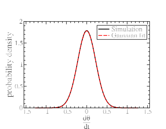
Figure -1256: Histogram of $\dot{\theta}$ from agent-based simulations for $M=35.349$ and $\Gamma=-0.1$ (black curve) compared with fitted Gaussian function (red curve) with variance $0.05$ whereas the measured value is $\langle\dot{\theta}^{2}\rangle=0.0506$. Parameters: $Sc=0.15$, linear system size $L=40$, $N=2000$, $v_{0}=2$, $R=3$, $M\,Sc^{2}=0.795211$, time step $\tau=0.025$, average over $40$ ensembles.

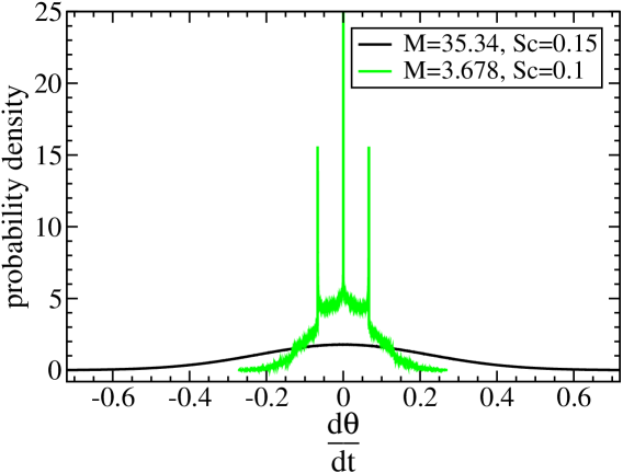
Figure -1255: Histogram of $\dot{\theta}$ from agent-based simulations for $M=3.678$ and $\Gamma=-0.06666$ (green curve). The central peak has a height of $212.3$. Parameters: $Sc=0.1$, linear system size $L=40$, $N=2000$, $v_{0}=2$, $R=3$, $M\,Sc^{2}=0.03677$, time step $\tau=0.025$, average over $40$ ensembles. Comparison with the measured distribution for $M=35.34$ and $Sc=0.15$ (black curve).

To proceed, we calculate the variance of $\dot{\theta}_{i}$ from the microscopic collision rule. Within our simple mean-field assumption we consider particles even within the collision circle as uncorrelated. This is in contrast to the more accurate one-sided molecular chaos approximation we employed at small density. Thus, we assume that the two-particle distribution function $P(\theta_{i},\theta_{j})=P(\theta_{i})P(\theta_{j})=1/(2\pi)^{2}$, factorizes and obtain the variance as,

$$\langle\dot{\theta}_{i}^{2}\rangle = \langle(-|\Gamma|\sum_{j\in\Omega_{i}}\sin(\theta_{j}-\theta_{i}))^{2}\rangle$$ (136)

$$= \Gamma^{2}\sum_{n=0}^{\infty}Prob(\#neighbors=n)\bigg{[}\sum_{j=2}^{n+1}\int_{0}^{2\pi}\sin^{2}(\theta_{j}-\theta_{i})\frac{1}{2\pi}d\theta_{j}$$

$$+ \sum_{j\neq k,=2}^{n+1}\int_{0}^{2\pi}\sin(\theta_{j}-\theta_{i})\frac{1}{2\pi}d\theta_{j}\int_{0}^{2\pi}\sin(\theta_{k}-\theta_{i})\frac{1}{2\pi}d\theta_{k}\bigg{]}$$

$$= \Gamma^{2}\sum_{n=0}^{\infty}Prob(\#neighbors=n)\sum_{j=2}^{n+1}\int_{0}^{2\pi}\sin^{2}(\theta_{j}-\theta_{i})\frac{1}{2\pi}d\theta_{j}$$

$$= \Gamma^{2}M\int_{0}^{2\pi}\sin^{2}(\theta_{j}-\theta_{i})\frac{1}{2\pi}d\theta_{j}=\frac{\Gamma^{2}M}{2}.$$

In section V.2, the validity of Eq. (136) is checked by agent-based simulations.

IV.3.2 The relation between $\langle\dot{\theta}^{2}\rangle$ and the velocity autocorrelation function

Differentiating the autocorrelation function, Eq. (126), with respect to time gives

$${dC(\tau)\over d\tau}=\dot{C}=-v_{0}^{2}\langle\dot{(\Delta\theta_{i})}\,{\rm sin}(\Delta\theta_{i})\rangle=-v_{0}^{2}\langle\dot{\theta}_{i}(t+\tau)\,{\rm sin}(\Delta\theta_{i})\rangle$$ (137)

For vanishing time interval, $\tau\rightarrow 0$, ${\rm sin}(\Delta\theta_{i})$ goes to zero and we find

$$\dot{C}|_{\tau=0}=0$$ (138)

Differentiating a second time results in

$${d^{2}C(\tau)\over d\tau^{2}}=\ddot{C}=-v_{0}^{2}\Big{[}\langle\ddot{\theta}_{i}(t+\tau)\,{\rm sin}(\Delta\theta_{i})\rangle+\langle\dot{\theta}^{2}_{i}(t+\tau)\,{\rm cos}(\Delta\theta_{i})\rangle\Big{]}$$ (139)

and we obtain a relation to the variance as

$$\ddot{C}|_{\tau=0}=-v_{0}^{2}\,\langle\dot{\theta}_{i}^{2}\rangle$$ (140)

For a Gaussian noise, the autocorrelation function has the form given by Eq. (130). Differentiating (130) and requiring consistency with (138) yields

$${d\over d\tau}\langle\Delta\theta_{i}^{2}\rangle|_{\tau=0}=0$$ (141)

whereas differentiating Eq. (130) a second time leads to

$$\ddot{C}\big{|}_{\tau=0}=-{v_{0}^{2}\over 2}\,{d^{2}\over d\tau^{2}}\langle\theta_{i}^{2}\rangle\big{|}_{\tau=0}$$ (142)

Comparison to (140) gives us a way to obtain the small time behavior of the angular displacement from the microscopic collision rule,

$${d^{2}\over d\tau^{2}}\langle\Delta\theta_{i}^{2}\rangle\big{|}_{\tau=0}=2\langle\dot{\theta}_{i}^{2}\rangle\big{|}_{\tau=0}=\Gamma^{2}\,M\,,$$ (143)

where Eq. (136) was used. Due to the requirements, (141) and (143), a linear time dependence of $\langle\Delta\theta_{i}^{2}\rangle$ as in perfect angular diffusion $\langle\Delta\theta_{i}^{2}\rangle\sim\tau$ is ruled out for small time scales $\tau<R/v_{0}$ but is expected to appear at larger times. This just reflects the fact that in reality no noise is perfectly white. Here, the effective dynamical noise is colored with a finite autocorrelation time of order $R/v_{0}$ which describes the arrival and departure of collision partner in the collision circle of a given particle. As we will see later, this small “non-whiteness” is essential for the long-time diffusive behavior of the displacement. According to (141) and (143), for small times, we expand the angular displacement as

$$\langle\Delta\theta_{i}^{2}\rangle=\tau^{2}{\Gamma^{2}M\over 2}+\alpha_{3}|\tau|\tau^{2}+\alpha_{4}\tau^{4}+\ldots$$ (144)

with coefficients $\alpha_{j}$ given later in Eq. (174).

IV.3.3 A random telegraph model

The main difficulty in solving the microscopic evolution equations for the angles $\theta_{i}$, Eqs. (135), is that although the equations can be formally closed, there is a dependence on the entire history of all the angles. This can be seen by integrating the position equations (1) and writing the indicator functions $a_{ij}$ as

$$a_{ij}(t)=a(|\vec{r}_{i}(t)-\vec{r}_{j}(t)|)=a\left(v_{0}\left|\int_{0}^{t}[\hat{n}(\theta_{i}(t^{\prime}))-\hat{n}(\theta_{j}(t^{\prime}))]\,dt^{\prime}\right|\right)$$ (145)

For low densities, the difficulty could be resolved by expressing the dynamics in terms of isolated two-particle meetings within a Boltzmann-like theory. However, to obtain a similar quantitative theory for moderate and high densities, one would have to abandon the one-sided molecular chaos assumption and to include a consistent treatment of two- or higher-particle correlation functions. In principle, this can be done by means of ring-kinetic theory chou_15 ; kuersten_21b or the less accurate Landau kinetic theory patelli_21 for active particles. However, these theories are very complicated and often they can only be evaluated with a numerical effort of the same or higher order as direct agent-based simulations. Therefore, in this paper, we adopt a drastically simplified theoretical approach: the quantities $a_{ij}$ in Eq. (135) which can only take the values zero or one, are modeled as independent random telegraph (RT) processes, see Appendix D,

$$\langle a_{ij}(t+\tau)\,a_{ij}(t)\rangle=\delta_{jk}\,g(\tau)\;\;\;{\rm for}\;i\neq j,\,i\neq k$$ (146)

with the correlation function $g(\tau)$ which is even in time, $g(\tau)=g(-\tau)$ and will be constructed from the microscopic details of the active particle system. Here, the focal particle $i$ is different from the particles $j$ and $k$ it “collides” with. This simplification decouples the dynamics of the angles from the neighbor property $a_{ij}$.

To derive an equation for the angular displacement and thus for the vaf, we define the following complex numbers at two different times $\tilde{t}$ and $t^{\prime}$:

$$z_{j} \equiv {\rm e}^{i\theta_{j}(t^{\prime})}$$

$$\tilde{z}_{j} \equiv {\rm e}^{i\theta_{j}(\tilde{t})}$$ (147)

Because of Eq. (127) we can write the mean square angular displacement as

$$\langle\Delta\theta_{i}^{2}\rangle = \int_{t}^{t+\tau}d\tilde{t}\int_{t}^{t+\tau}dt^{\prime}\langle\dot{\theta}(\tilde{t})\,\dot{\theta}(t^{\prime})\rangle$$ (148)

$$= \Gamma^{2}\int_{t}^{t+\tau}d\tilde{t}\int_{t}^{t+\tau}dt^{\prime}\sum_{j=1}^{N}\sum_{k=1}^{N}\langle a_{ij}(\tilde{t})\,a_{ik}(t^{\prime})\,{\rm sin}(\tilde{\theta}_{j}-\tilde{\theta}_{i})\,{\rm sin}(\theta_{k}-\theta_{i})\rangle$$

with the abbreviations $\tilde{\theta}_{j}\equiv\theta_{j}(\tilde{t})$ and $\theta_{j}\equiv\theta_{j}(t^{\prime})$. Assuming that the $a_{ij}$ are independent of the angles with a second moment given by Eq. (146), and using the complex representation of the sine, one finds

$$\langle\Delta\theta_{i}^{2}\rangle=-{\Gamma^{2}\over 4}\sum_{j=1}^{N}\int_{t}^{t+\tau}d\tilde{t}\int_{t}^{t+\tau}dt^{\prime}g(\tilde{t}-t^{\prime})\langle(\tilde{z}_{j}\tilde{z}_{i}^{*}-\tilde{z}_{i}\tilde{z}_{j}^{*})(z_{j}z_{i}^{*}-z_{i}z_{j}^{*})\rangle$$ (149)

In evaluating the right hand side of (149) we assume that particles are uncorrelated (Molecular chaos assumption), that is, for example, $\langle\tilde{z}_{j}z_{i}^{*}\rangle=\langle\tilde{z}_{j}\rangle\langle z_{i}^{*}\rangle=0$ or $\langle\tilde{z}^{*}_{j}z_{j}\tilde{z}_{i}z_{i}^{*}\rangle=\langle\tilde{z}^{*}_{j}z_{j}\rangle\langle\tilde{z}_{i}z_{i}^{*}\rangle$. We also assume isotropy, i.e. that there is no preferered direction. This means that combinations of the $z_{j}^{\prime}s$ and $\tilde{z}_{j}^{\prime}s$ which are not rotationally invariant, such as $z_{j}\tilde{z}_{j}$ have a vanishing mean value, e.g. $\langle z_{j}\tilde{z}_{j}\rangle=0$. This can be seen by rotating the coordinate system by an arbitrary angle $\alpha$. The combination $z_{j}\tilde{z}_{j}$ would turn into ${\rm exp}(2i\alpha)z_{j}\tilde{z}_{j}$ i.e. would have an explicit dependence on the orientation of the coordinate system, and thus is not rotationally invariant. In contrast, rotating the combination $z^{*}_{j}\tilde{z}_{j}$ would show no such dependence. Note, that the $N(N-1)$ terms proportional to terms $\langle a_{ij}\rangle\langle a_{ik}\rangle$ for $j\neq k$ in (148) have prefactors that vanish under the presumed Molecular chaos assumption.

Finally, since all $j=1\ldots N$ particles have identical properties and since for $j=i$ there is no contribution to the right hand side, we obtain

$$\langle\Delta\theta_{1}^{2}\rangle={\Gamma^{2}(N-1)\over 4}\int_{t}^{t+\tau}d\tilde{t}\int_{t}^{t+\tau}dt^{\prime}g(\tilde{t}-t^{\prime})\Big{[}\langle\tilde{z}_{2}z_{2}^{*}\rangle\langle\tilde{z}^{*}_{1}z_{1}\rangle+\langle\tilde{z}^{*}_{2}z_{2}\rangle\langle\tilde{z}_{1}z^{*}_{1}\rangle\Big{]}$$ (150)

where we took particle $i=1$ as focal particle and particle $j=2$ as a representative neighbor of particle $1$. Using the Gaussian assumption for the angular displacements we can express the products on the right hand side of (150) as given in Eq. (128). For example, one has

$$\langle\tilde{z}^{*}_{1}z_{1}\rangle=\Big{\langle}{\rm e}^{i[\theta_{1}(t^{\prime})-\theta_{1}(\tilde{t})]}\Big{\rangle}={\rm e}^{-{1\over 2}\langle\Delta\theta_{1}^{2}(\tilde{t}-t^{\prime})\rangle}=\langle\tilde{z}_{1}z^{*}_{1}\rangle$$ (151)

Requiring self-consistency, we drop the particle indices, since every particle’s displacement should be the same on average. Assuming stationarity and by formally going to the thermodynamic limit, $N\rightarrow\infty$, $L\rightarrow\infty$ at constant $\rho_{0}=N/L^{2}$, we obtain an integral equation for the mean angular displacement,

$$\langle\Delta\theta^{2}(\tau)\rangle={\Gamma^{2}\over 2}\int_{0}^{\tau}d\tilde{t}\int_{0}^{\tau}dt^{\prime}\,\hat{g}(\tilde{t}-t^{\prime})\,{\rm e}^{-\langle\Delta\theta^{2}(\tilde{t}-t^{\prime})\rangle}$$ (152)

with the scaled correlation function $\hat{g}$ of the random telegraph process,

$$\hat{g}(t)=\lim_{N\rightarrow\infty}(N-1)\,g(t)$$ (153)

This correlation function is calculated in Appendix D with the result

$$\hat{g}(\tau)=M{\rm e}^{-w_{off}\,|\tau|}$$ (154)

Here, $w_{off}$ is the rate by which the random variable $a_{ij}$ switches from one to zero. Thus, $w_{off}$ parametrizes the statistical modelling of the effect that a collision partner of the focal particle leaves the collision circle at a particular time. This connection to the microscopic dynamics will be made explicit in the following sections where $w_{off}$ will be determined self-consistently by means of kinetic theory. Inserting Eq. (154) into (152) leads to the final form of the integral equation for the mean square angular displacement

$$\langle\Delta\theta^{2}(\tau)\rangle={\Gamma^{2}M\over 2}\int_{0}^{\tau}d\tilde{t}\int_{0}^{\tau}dt^{\prime}\,{\rm e}^{-w_{off}|\tilde{t}-t^{\prime}|}\,{\rm e}^{-\langle\Delta\theta^{2}(\tilde{t}-t^{\prime})\rangle}\,.$$ (155)

Solving this self-consistent equation for the function $\langle\Delta\theta^{2}(\tau)\rangle$ allows us to find the velocity auto-correlation function $C(\tau)$ at all times $\tau$ by means of Eq. (130). A similar integral equation has been found earlier in Ref. vanmeegen_18 in the context of randomly coupled but fixed rotators. As shown later, knowledge of the mean square angular displacement enables the calculation of the noise correlations $\langle\xi(t)\xi(t^{\prime})\rangle$ by inverting Eq. (129).

IV.3.4 Calculating the rate $w_{off}$

The determination of the OFF-rate, $w_{off}$ is essential for a good model of the collision process by the random telegraph process. We consider the event that the variable $a_{ij}$ takes the value zero for the first time after having started from the value one at time $t=0$. The probability that this occurs at a time between $t$ and $t+dt$ is denoted by $W_{1\rightarrow 0}=P_{1\rightarrow 0}(t)\,dt$. To find the probability density $P_{1\rightarrow 0}$ for the random telegraph process, we discretize time $t=t_{n}=n\,\Delta t$ with a small time step $\Delta t$. The probability for the first “success” (corresponding to switching from 1 to 0 for the first time) at time $t_{n}$ is given by the geometric discribution:

$$W_{n}=(1-w_{off}\Delta t)^{n-1}\,w_{off}\,\Delta t=\left(1-{w_{off}t_{n}\over n}\right)^{n-1}\,w_{off}\,\Delta t$$ (156)

Setting $W_{n}=P_{1\rightarrow 0}(t)\,\Delta t$ and performing the continuous time limit $\Delta t\rightarrow 0$ at fixed time $t=t_{n}$ and using the relation

$$\lim_{n\rightarrow\infty}\left(1-{x\over n}\right)^{n}={\rm e}^{-x}$$ (157)

gives

$$P_{1\rightarrow 0}(t)=w_{off}{\rm e}^{-w_{off}\,t}$$ (158)

This exponential probability density has a finite mean: The averaged first passage time for the flip from ON to OFF follows as

$$T_{flip}=\langle t\rangle=\int_{0}^{\infty}t\,P_{1\rightarrow 0}(t)\,dt={1\over w_{off}}$$ (159)

because the density $P_{1\rightarrow 0}(t)$ is normalized to one.

To determine $w_{off}$ and to provide a link to the random telegraph process, we first consider the actual contact process of a particle that has entered the collision circle of the focal particle $i=1$ at time zero and leaves it at time $t$. As a first approximation, we assume that $Sc=|\Gamma|R/v_{0}\rightarrow 0$, which means that particles move ballistically in straight lines with constant speed during their contact time. Assuming furthermore that particles outside the collision circle are equally distributed in space and have no preferred direction, the average contact time turns out to be finite as in the RT-process and can be calculated exactly by means of kinetic theory, as shown in Appendix E, with the result

$$\langle t\rangle={\pi^{2}\over 8}{R\over v_{0}}$$ (160)

Equating this moment with the one from the RT-process, Eq. (159), leads to the OFF-rate,

$$w_{off}=B\,{v_{0}\over R}$$ (161)

with the constant $B=8/\pi^{2}\approx 0.81$. The behavior that $w_{off}\sim R/v_{0}$ with a proportionality constant of order one is expected on dimensional and physical grounds since the time a particle of speed $v_{0}$ flies through an area of linear extension $R$ is of order $R/v_{0}$. Modeling by the random telegraph process is not perfect as indicated by the fact that the distribution of the exit time $t_{exit}$ is qualitatively different from the actual behavior of particles in the limit $Sc\rightarrow 0$. According to Eq. (247) the distribution for the direct contact process has a power law tail, whereas in the RT-process the distribution is exponential. As a consequence, while the scaling behavior of $w_{off}$ is captured correctly, the prediction for the prefactor $B$ should only be taken as a first estimate. In chapter IV.3.7 it is shown how $B$ can determined self-consistently by matching it to the Boltzmann-like kinetic theory with the result $B=9\pi^{2}/64$.

IV.3.5 Solution of the integral equation

All parameters in the non-linear integral equation (155) for the mean square angular displacement are defined and we proceed to solving it. First, we discretize time with a small time step $\Delta t$ as $\tilde{t}=n\,\Delta t$, $t^{\prime}=m\,\Delta t$, $\tau=p\,\Delta t$ with $n,m,p=0,1,2,\ldots$ and define $\langle\Delta\theta(\tau)^{2}\rangle=\langle\Delta\theta(p\,\Delta t)^{2}\rangle\equiv x_{p}$. The integral equation (155) is then discretized as

$$x_{p}={M\Gamma^{2}\over 2}\Delta t^{2}\sum_{n=1}^{p}\sum_{m=1}^{p}{\rm e}^{-w_{off}\,\Delta t|n-m|-x_{n-m}}\;\;\;\;{\rm for}\;p\geq 1$$ (162)

with initial value $x_{0}=0$ and where we imply the discrete time-reversal symmetry $x_{n-m}=x_{m-n}$. At the smallest non-zero time, $p=1$, Eq. (162) reproduces the quadratic small time behavior required by Eq. (144), $x_{1}={M\Gamma^{2}\over 2}\,\Delta t^{2}$.

By increasing $p$ step by step, we found a simpler form of the discretized integral equation

$$x_{p}={M\Gamma^{2}\Delta t^{2}\over 2}\Big{[}p+2\sum_{m=1}^{p-1}(p-m)\,{\rm e}^{-m\,w_{off}-x_{m}}\Big{]}$$ (163)

Because the right hand side of (163) contains only displacements $x_{m}$ at smaller times, i.e. with $m<p$, it is a recurrence relation for the value of $x_{p}$ using the values $x_{p-1},x_{p-2},\ldots x_{0}$. Thus, by inreasing the index $p$ in steps of one, storing all obtained values $x_{p}$ for use in the next sweep, the entire temporal behavior of the angular displacement can be found numerically, see Fig. -1254. Numerical results obtained by this method in Fig. -1254 show that $x_{p}$ increases linear in time at large times, corresponding to a simple exponential decay of the vaf, see (130).

Figure -1254: The normalized angular displacement $\langle\Delta\theta^{2}\rangle/\epsilon$ is plotted versus dimensionless time $\tilde{t}=t\,w_{off}$. The black curve shows the numerical solution of the integral equation (163), whereas the red line is the analytical linear result from Eq. (173), given here by $-0.99+0.99995\,\tilde{t}$. Parameters: $\epsilon=0.01$, $wt=\Delta t\,w_{off}=0.001$, $N_{tot}=5\times 10^{4}$ points, $M=1$, $|\Gamma|/w_{off}=0.1$.

Performing the continuum limit of the recurrence relation (163) by $\sum\Delta t\ldots\rightarrow\int\,dt\ldots$ for $\Delta t\rightarrow 0$ we arrive at a simpler integral equation,

$$\langle\Delta\theta(\tau)^{2}\rangle=M\Gamma^{2}\int_{0}^{\tau}\,(\tau-t)\,{\rm e}^{-w_{off}\,t-\langle\Delta(t)^{2}\rangle}\,dt\,.$$ (164)

Differentiating Eq. (164) or (155) twice with respect to $\tau$ leads to a non-linear differential equation for $x(t)\equiv\langle\Delta\theta^{2}(t)\rangle$ with explicit time dependence,

$$\ddot{x}(t)=M\Gamma^{2}{\rm e}^{-w_{off}\,|t|-x(t)}\,.$$ (165)

The explicit time dependence in the differential equation (165) can be eliminated for $t\neq 0$ by the transformation

$$y=x+w_{off}\,|t|$$ (166)

to yield

$$\ddot{y}(t)=M\Gamma^{2}{\rm e}^{-y(t)}+2\,w_{off}\,\delta(t)$$ (167)

with $\gamma\equiv M\Gamma^{2}$ because of $\dot{y}=\dot{x}+2\,w_{off}[\theta(t)-1/2]$ and $\ddot{y}=\ddot{x}+2w_{off}\delta(t)$. Eq. (167) can be interpreted as the equation of motion of a particle in an effective potential. Multiplying by $\dot{y}$ and integrating in time one finds the corresponding conserved “energy” of this motion:

$$E=const={\dot{y}^{2}\over 2}+\gamma{\rm e}^{-y}$$ (168)

Because of the initial conditions $x(t=0)=0$ and $\dot{x}(0)=0$, one has $y(t=0)=0$ and $\dot{y}(t=0)=w_{off}$ which gives the value of the generalized energy, $E=\gamma+w_{off}^{2}/2$. Solving Eq.(168) for the function $t(y)$ leads to

$$t=\int_{0}^{y}\left[2\gamma\left(1-{\rm e}^{-x}\right)+w_{off}^{2}\right]^{-1/2}\,dx$$ (169)

The transformation ${\rm exp}(-x)=z^{2}$ leads to a solvable standard integral,

$$t=-\sqrt{2\over\gamma}\int_{1}^{{\rm exp}(-y/2)}{dz\over z\sqrt{a^{2}-z^{2}}}$$ (170)

with $a^{2}\equiv 1+w_{off}^{2}/(2\gamma)=1+1/(2\epsilon)$ and $\epsilon=M\Gamma^{2}/w_{off}^{2}$. One obtains

$$t=\left.\sqrt{2\over\gamma a^{2}}\,{\rm ln}\left({a+\sqrt{a^{2}-z^{2}}\over z}\right)\right|_{1}^{{\rm exp}(-y/2)}=\sqrt{2\over\gamma a^{2}}\,{\rm ln}\left({\left[a+\sqrt{a^{2}-{\rm exp}(-y)}\right]{\rm exp}(y/2)\over a+\sqrt{a^{2}-1}}\right)$$ (171)

Defining the variable $z\equiv{\rm exp}(-y/2)$ leads to a quadratic equation for $z$, which is, of course, solvable. Thus, finally, it turns out that the integral equation (155) as well as the differential equation (165) are exactly solvable, and the angular displacement follows as

$$x(t)=2{\,\rm ln}\left\{{c^{2}+{\rm e}^{-2\lambda\,|t|}\over 2b\,c\ {\rm e}^{-\lambda|t|}}\right\}-w_{off}|t|$$ (172)

with $\epsilon\equiv\gamma/w_{off}^{2}$, $b^{2}\equiv 1+1/2\epsilon$, $c\equiv b+\sqrt{b^{2}-1}$, $\lambda=w_{off}\,b\sqrt{\epsilon/2}$.

The solution is rewritten in terms of the dimensionless time $\tilde{t}=t\,w_{off}$ and the scaled angular displacement $\tilde{x}=x/\epsilon$. Analysis for $\tilde{t}\gg 1$ allows neglecting esponentially small terms $\sim{\rm exp}(-\tilde{t})$ and gives the expected simple linear growth of the displacement at large times:

$$\tilde{x}={\sqrt{1+2\epsilon}-1\over\epsilon}\,\tilde{t}-{2\over\epsilon}\,{\rm ln}\left[{2\sqrt{1+2\epsilon}\over 1+\sqrt{1+2\epsilon}}\right]$$ (173)

In Fig. -1254 one sees excellent agreement of this asymptotic behavior with the full exact solution. We checked that the analytical solution (172) agrees perfectly with the numerical solution of the integral equation (163).

For completeness, a perturbative solution of the differential equation (165) for small times will be given here in dimensionless form,

$$\tilde{x}={1\over 2}\tilde{t}^{2}-{1\over 6}|\tilde{t}|^{3}+{1\over 2}\left[{1\over 2}-\varepsilon\right]\tilde{t}^{4}+{1\over 40}\left[\varepsilon-{1\over 3}\right]|\tilde{t}|^{5}+O(\tilde{t}^{6})\,$$ (174)

where the first, quadratic, term agrees with the expectation, Eq. (144).

IV.3.6 Calculating the noise correlations

Differentiating Eq. (129) twice with respect to $\tau$ gives the relation between the noise correlations and the angular displacement $x(\tau)=\langle[\Delta\theta(\tau)]^{2}\rangle$,

$$\ddot{x}(\tau)=2\,\langle\xi(t)\xi(0)\rangle$$ (175)

From (165) we know how to express $\ddot{x}$ in terms of $x$ and $y$,

$$\langle\xi(t)\xi(0)\rangle={\gamma\over 2}{\rm e}^{-y}$$ (176)

where $y=x+w_{off}|t|$ and inserting the solution for $x$ from (172) we obtain an explicit expression for the noise correlations

$$\langle\xi(t)\xi(\tilde{t}\rangle={\gamma\over 2}\left[{2\,b\,c\,{\rm e}^{-\lambda|t-\tilde{t}|}\over c^{2}+{\rm e}^{-2\lambda|t-\tilde{t}|}}\right]^{2}$$ (177)

As shown in Fig. -1252, the correlations become exponential for $|\tau|\gtrapprox R/v_{0}$. When coarse-graining on time scales of order $R/v_{0}$ (as done in the Boltzmann-like kinetic theory), the colored network noise appears as an effective white noise, $\langle\xi(\tau)\xi(0)\rangle\sim\sigma^{2}\delta(\tau)$. To calculate its strength $\sigma^{2}$ we integrate the noise correlations from zero to a very large time $T$. For an assumed white noise this gives

$$\int_{0}^{T}\langle\xi(t)\xi(\tilde{0}\rangle\,dt={\sigma^{2}\over 2}$$ (178)

whereas from (175) it follows

$$\int_{0}^{T}\langle\xi(t)\xi(\tilde{0}\rangle\,dt=\int_{0}^{T}{\ddot{x}\over 2}\,dt={1\over 2}\dot{x}(T)$$ (179)

Equating the two results and performing the limit $T\rightarrow\infty$, we obtain the strength of the equivalent white noise as

$$\sigma^{2}=\lim_{T\rightarrow\infty}\dot{x}(T)=\gamma\int_{0}^{\infty}{\rm e}^{-x(\tau)-w_{off}\tau}\,d\tau=w_{off}\left[\sqrt{1+2\epsilon}-1\right]$$ (180)

Because of $\tau_{C}=2/\sigma^{2}$, see Eq. (134), the RT-model predicts the auto-correlation time as

$$\tau_{C}={2\over w_{off}\left[\sqrt{1+2\epsilon}-1\right]}$$ (181)

Note, that in the thermodynamic limit the ratio $M/N$ goes to zero, and the effective noise $\sigma^{2}$ only depends on the OFF-rate $w_{off}$ of the random telegraph process.

IV.3.7 Matching the random-telegraph model and the Boltzmann-like theory

Eqs. (180, 181) suggest that the noise strength $\sigma^{2}$ and the auto-correlation time $\tau_{C}$ are solely controlled by the composite variable $\epsilon\sim MS^{2}$. As shown in Fig. (-1253), this is consistent with agent-based simulations: all data points for $\tau_{C}$ approximately lie on a Master curve when plotted versus $M\,Sc^{2}$. Under this assumption, expression (134) from kinetic theory, valid for $M\ll 1$ and $Sc\ll 1$, should match the small $\epsilon$ limit of (180). This is indeed the case and fixes the proportionality constant in the Ansatz $w_{off}=B\,v_{0}/R$ to the value

$$B={9\pi^{2}\over 64}\approx 1.38791\,.$$ (182)

This leads to the final theoretical prediction for $\tau_{C}$ and the self-diffusion coefficient $D$,

$$\tau_{C} = {128R\over 9\pi^{2}v_{0}}\,\left[\sqrt{1+{8192\,M\,Sc^{2}\over 81\pi^{4}}}-1\right]^{-1}$$ (183)

$$D = {64v_{0}R\over 9\pi^{2}}\,\left[\sqrt{1+{8192\,M\,Sc^{2}\over 81\pi^{4}}}-1\right]^{-1}\,,$$ (184)

supposedly valid for all densities $M$ but for small $Sc\ll 1$. Plotting this prediction in Fig. (-1253) shows excellent agreement with agent-based results at small $MS^{2}$. At larger $M$ or $Sc$, the theory underestimates the correlation time $\tau_{C}$, probably because the random-telegraph theory neglects correlations among particles inside the collision circle. Since there are more such particles at larger $M$, these neglected contributions carry more weight in the final expression. Furthermore, the determination of the coefficient $B$ was based on the Boltzmann-like kinetic theory which was only evaluated up to $O(Sc^{2})$. Thus, deviations for $Sc>1$ are also not surprising. However, modifications of the value of $B$ will not be sufficient to remedy the strong deviation between theoretical predictions and simulations at large $M\,Sc^{2}$ by about a factor of ten. This is because in this limit, the expression (181) for $\tau_{C}$ becomes independent of $B$,

$$\tau_{C}=\sqrt{2\over M}\,{1\over|\Gamma|}\;\;\;{\rm for}\,M\,Sc^{2}\gg 1$$ (185)

Possible reasons for the discrepancies at larger $M\,Sc^{2}$ will be investigated in section V.2 in more detail.

Figure -1253: The scaled auto-correlation time $\tau_{C}\,v_{0}/R$ from agent-based simulations versus the scaling variable $\delta=M\,Sc^{2}$ for different values of $M$, compared to the theoretical prediction, Eq. (183).

Figure -1252: The theoretical prediction for the scaled noise correlations $\langle\xi(t)\xi(0)\rangle/M\Gamma^{2}$ according to Eq. (177) versus scaled time $\tilde{t}=tv_{0}/R$ for different values of the variable $M\,Sc^{2}=0.01$ (black), $0.1$ (red) till $M\,Sc^{2}=10$ (orange). For $\tilde{t}\lessapprox 0.7$, the correlations are non-exponential.

V Numerics

V.1 The relaxation of angular modes

Figure -1251: Relaxation of the first angular modes $\hat{f}_{k}$, divided by $\hat{f}_{0}$, as a function of dimensionless time $\tilde{t}=t\,|\Gamma|$, obtained by agent-based simulations (solid lines), Vlasov-like mean-field theory (dotted lines), and Boltzmann-like kinetic theory (dashed lines) for $Sc=0.05$ and $M=0.1$. Parameters for the agent-based simulations: $N=493$ particles, $\Gamma=-0.2$, integration time step $dt=0.025$, $v_{0}=4$, $R=1$, linear system size $L=124$, inital opening angle $\alpha=150^{o}$, number of replicas in the ensemble average, $n_{ens}=100$.

The usual hydrodynamics modes, particle density and momentum density, are encoded in the lowest angular modes $\hat{f}_{0}$ and $\hat{f}_{1}$. The higher modes $\hat{f}_{2},\hat{f}_{3},\ldots$ relax faster and are thus considered kinetic modes. It is interesting to see to if the Vlasov- and Boltzmann-like theories introduced above are able to correctly describe the time-evolution of the angular modes, even far away from stationary states. Here, we will restrict ourselves to homogeneous systems and leave the evaluation of the full spatiotemporal behavior for future research.

We performed agent-based simulations by solving the time-discretized versions of Eqs. (1,2) for $N$ particles using a small time step $\tau$ on a quadratic domain of linear size $L$ with periodic boundary conditions. The system was initialized by randomly placing particles on the domain with flying directions which are equally distributed in the interval $[-\alpha/2,\alpha/2]$ with respect to the x-axis. The angular parameter $\alpha>0$ was chosen to be significantly smaller than $2\pi$. Thus, the initial state is spatially homogeneous but ordered where all angular Fourier modes are excited according to

$$\hat{f}_{k,init}={\rho_{0}\over 2\pi}\int_{0}^{2\pi}P(\theta){\rm e}^{-ik\theta}\,d\theta={\rho_{0}\over 2\pi\alpha}\int_{-\alpha/2}^{\alpha/2}{\rm e}^{-ik\theta}\,d\theta={\rho_{0}\over 2\pi}\,{\rm sinc}\left({\alpha k\over 2}\right)$$ (186)

which follows from the definition (11), and where $P(\theta)$ is the angular distribution of a single particle, and $\rho_{0}=N/L^{2}$. The temporal evolution of the the particles was calculated and the instantaneous angular Fourier modes were measured as

$$\hat{f}_{k}(t)={\rho_{0}\over 2\pi}{1\over N}\sum_{j=1}^{N}{\rm e}^{-ik\theta_{j}(t)}$$ (187)

These measurements were repeated on replica systems which were initialized in the same way but with different random seeds, and an ensemble average of the Fourier modes was performed. Fig. -1251 shows the relaxation of the first modes, $\hat{f}_{1}$, $\hat{f}_{2}$ and $\hat{f}_{3}$. As expected the higher modes relax faster. After a sufficiently long time, all modes had relaxed to zero, corresponding to a disordered stationary state. The non-monotonic decay of the mode $\hat{f}_{2}$ which describes nematic order can be understood as follows: Initially, the particles fly mostly in the x-direction, corresponding to relatively large positive values of the polar and nematic order parameter, $\hat{f}_{1}$ and $\hat{f}_{2}$, respectively. Due to the anti-aligment interaction, particles turn away from each other where about half of the particles tend to go towards the y-direction, whereas the other half goes more towards the negative y-direction. This splitting corresponds to small polar order but significant nematic order with a negative value of $\hat{f}_{2}$, eventually reaching the minimum value of $\hat{f}_{2}$. Later on, while attempting to turn anti-parallel to their repective neighbors, the particles get completely mixed and disoriented, and thus all $\hat{f}_{k}$ with $k\geq 1$ go to zero.

To compare this behavior with the predictions from kinetic theory, we also solved the hierarchy equations, Eqs. (12) for the Vlasov-like hierarchy, and the Boltzmann-like hierarchy where the additional collision term from Eq. (108) was added to the right hand side of (12). The equations for the first 48 modes were solved explicitly where all higher modes were set to zero. We checked, that a truncation at a slightly different mode number does no significantly change the results.

Fig. -1251 shows that at small times both kinetic theories agree very well with the agent-based result. However, at larger times, the regular mean-field results start deviating from the direct simulations. Finally, at large times, a qualitatively different behavior is apparent: the angular modes do not converge to zero but non-zero asymptotic values are reached, meaning that the stationary state is ordered. In addition, by changing the initial opening angle $\alpha$, we observed that the actual asymptotic values depend on $\alpha$, i.e. on the initial conditions.

In contrast, the addition of the small correction due to non-mean field effects to the Vlasov-like collision operator introduces a new long time scale, $\tau_{long}=(R/v_{0})/M\,Sc^{2}$, which describes the final relaxation of all modes to zero and is very large at low densities and coupling strengths. Furthermore, this small modification leads to an excellent, quantitative agreement between the Boltzmann-like kinetic theory and the agent-based simulations. As expected, this agreement gets better, the smaller the scaled density $M$ and the smaller the coupling strength $Sc$ is. For large $M>1$, the assumptions of a Boltzmann-like theory are not valid. However, the qualitative picture stays the same: the system eventually becomes disordered, which is confirmed by the improved kinetic theory but not by the Vlasov-like theory.

We conclude that in our noise-free system, the regular mean-field approximation of factorizing the N-particle probability distribution leads to erroneous predictions, both at small and at large density, and should be abondoned. Instead, the one-sided molecular chaos approximation, as first used about 100 years ago in the standard Boltzmann-equation, leads to quantitatively correct results, at least in the low density limit.

V.2 Checking assumptions: measuring $\langle\dot{\theta}^{2}\rangle$

In the derivation of the self-consistent integral equation (155) that leads to the determination of the vaf in the limit of large $M$, a number of approxiations had to be made. One of them was a mean-field assumption in the calculation of $\langle\dot{\theta}^{2}\rangle$. In agent-based simulations we checked whether the result, Eq. (136), is actually correct. We found that it is quite accurate at small $M$ and $Sc$ but deviates increasingly for increasing $M$ which is not very encouraging as the result is needed in evaluating the large density case. For example, for $M=35.34$, see Fig. -1256 we observe $\langle\dot{\theta}^{2}\rangle/(M\Gamma^{2}/2)=0.28633$, i.e. the variance of the angular change is more than a factor of three smaller than predicted by the Molecular Chaos assumption. To rule out that this has to do with the average number of particles, we measured this independently with the result that the average number of neighbors is only a factor of $0.9633$ smaller than $M$. For a smaller density, $M=3.677$, see Fig. -1255, the difference is not so dramatic. Here, we find $\langle\dot{\theta}^{2}\rangle/(M\Gamma^{2}/2)=0.68334$ and an average neighbor number of $0.91407\,M$. Simulations at very large $M=123.7$, $Sc=0.1$ and $N=7000$ resulted in $\langle\dot{\theta}^{2}\rangle/(M\Gamma^{2}/2)=0.4341194$. F. For even larger $M=135.7$ and $Sc=0.15$ ($M\,Sc^{2}=3.054$) this ratio was measured at $\langle\dot{\theta}^{2}\rangle/(M\Gamma^{2}/2)=0.4483190$.

This lead us to the hypothesis that for larger $M$, different particles within the collision circle of particle $i$ are significantly anti-correlated. This causes relevant contributions of the $n(n-1)$ cross-terms $\sim\langle{\rm sin}(\theta_{j}-\theta_{i})\,{\rm sin}(\theta_{j}-\theta_{i})\rangle$ in Eq. (136), effectively lowering the impact of the $n$ diagonal contributions. The variance $M\Gamma^{2}/2$ is the essential parameter in the analysis of the RT-approach. Lowering it means that for the predicted relaxation times $\tau_{C}$ one should assign values that correspond to much lower $M$ in the ideal theory (based on Molecular chaos) which then leads to much larger predicted values of $\tau_{C}$.

It is interesting to note, that these cross-correlations cannot occur in the small density limit, $M\ll 1$ because in this case there is simply almost never a third particle involved in collisions. We speculate that the increasing relevance of the anti-correlations at larger $M$ is due to the fact that there is $n-1$ times more cross-terms than diagonal terms, and larger $n$ become more likely at a larger average value $M=\langle n\rangle$.

Since a self-consistent theory merely for the autocorrelation of a particle, such as Eq. (155), is apparently not sufficient for $M\,Sc^{2}>0.01$, one could expand the theory by an equation for the cross-correlations or set up a ring-kinetic theory. However, this is beyond the scope of this paper and will be left for future work.

VI Conclusions

In summary, we consider a model of self-propelled particles with anti-alignment interactions but without external noise. Starting at the N-particle Liouville equation and assuming low densities, we derive an asymptotically exact scattering theory by means of a non-local closure of the first BBGKY-equation. By means of this kinetic theory and a mapping to a random-telegraph process we construct an effective Langevin equation for the time evolution of a focal particle in a sea of host particles, which should be valid at arbitrary densities. Analytical expressions for the temporal correlations of its effective noise term and the corresponding self-diffusion coefficient are provided. The mathematical details of all derivations are laid out and the underlying assumptions are thoroughly discussed. Comparing to agent-based simulations we show that the theory accurately describes the time-evolution of the hydrodynamic and kinetic modes of the system, even far from stationary states. We demonstrate that the usual mean-field approach of Molecular Chaos which is based on a factorization of the N-particle probability density, fails in this deterministic system and leads to unphysical predictions such as an infinite coefficient of self-diffusion. The proposed theory opens a way to analytically treat other active systems beyond mean field, such as mixtures of different SPPs and models with non-reciprocal, chiral, and nematic interactions.

The main technical results of this paper are (i) the coupling matrix $g_{mn}$, Eq. (109), for the Fourier-modes which describe the extension of the Vlasov-like theory beyond mean field, (ii) the integral- and corresponding differential equations for the angular displacement, Eqs. (155, 165), (iii) the noise correlations of the effective network noise, Eq. (177), and (iv) the expression for the self-diffusion coefficient, Eq. (184).

Appendix A Two-particle scattering

The evolution equations for the angles of two interacting particles are

$$\dot{\theta}_{1} = \Gamma\,{\rm sin}(\theta_{2}-\theta_{1})$$ (188)

$$\dot{\theta}_{2} = \Gamma\,{\rm sin}(\theta_{1}-\theta_{2})$$ (189)

We define the auxiliary varibles,

$$\Delta \equiv \theta_{2}-\theta_{1}$$

$$\tilde{c} \equiv \theta_{1}+\theta_{2}\,.$$ (190)

By adding and subtracting equations (188, 189) one finds

$$\dot{\tilde{c}} =0$$ (191)

$$\dot{\Delta} =-2\Gamma\,{\rm sin}(\Delta)$$ (192)

Defining the angles $\alpha_{1}$ and $\alpha_{2}$ with respect to the vector $-\Delta\vec{r}=\vec{r}_{1}-\vec{r}_{2}$, see Fig. -1257, we have

$$\theta_{1} = \alpha_{1}+\beta$$

$$\theta_{2} = \alpha_{2}+\beta$$ (193)

and thus, $\Delta=\theta_{2}-\theta_{1}=\alpha_{2}-\alpha_{1}$ and

$$c\equiv\alpha_{1}+\alpha_{2}=\tilde{c}-2\beta\,.$$ (194)

Even though $\tilde{c}$ is conserved, the quantity $c$ depends on time. This is because during a collision of finite duration, the positions of the particles change, resulting in a change of the angle $\beta$ which is defined in Fig.  -1257.

The solution of the differential equation (192) is

$${\rm tan}\Big{[}{\Delta(\tilde{t})\over 2}\Big{]}={\rm tan}\Big{[}{\Delta(t)\over 2}\Big{]}\,{\rm exp}\big{[}2\Gamma(t-\tilde{t})\big{]}$$ (195)

The time evolution of the connecting vector $\Delta\vec{r}=(\Delta r_{x},\Delta r_{y})$ follows from integrations of Eq.(1) over time as

$$\Delta r_{x}(\tilde{t})-\Delta r_{x}(t) = v_{0}\int_{t}^{\tilde{t}}d\hat{t}\big{[}{\rm cos}(\theta_{2}(\hat{t}))-{\rm cos}(\theta_{1}(\hat{t}))\big{]}=-2v_{0}\int_{t}^{\tilde{t}}d\hat{t}\,{\rm sin}{\tilde{c}\over 2}\,{\rm sin}{\Delta(\hat{t})\over 2}$$

$$\Delta r_{y}(\tilde{t})-\Delta r_{y}(t) = v_{0}\int_{t}^{\tilde{t}}d\hat{t}\big{[}{\rm sin}(\theta_{2}(\hat{t}))-{\rm sin}(\theta_{1}(\hat{t}))\big{]}=2v_{0}\int_{t}^{\tilde{t}}d\hat{t}\,{\rm cos}{\tilde{c}\over 2}\,{\rm sin}{\Delta(\hat{t})\over 2}\,.$$ (196)

With the abbreviation

$$G\equiv\int_{t}^{\tilde{t}}d\hat{t}\,{\rm sin}{\Delta(\hat{t})\over 2}$$ (197)

and using the invariance of $\tilde{c}=\theta_{1}+\theta_{2}$, the evolution of the square of the distance between the particles $(\Delta r)^{2}=(\Delta r_{x})^{2}+(\Delta r_{y})^{2}$ follows from Eq. (196) as

$$(\Delta r(\tilde{t}))^{2}=(\Delta r(t))^{2}+4v_{0}^{2}G^{2}+4v_{0}G\Big{\{}\Delta r_{y}(t){\rm cos}{\tilde{c}\over 2}-\Delta r_{x}(t){\rm sin}{\tilde{c}\over 2}\Big{\}}$$ (198)

Expressing the connecting vector in polar coordinates at the exit time, where $|\Delta\vec{r}(t)|=R$,

$$\Delta r_{x}(t)=R\,{\rm cos}(\pi+\beta(t))=-R\,{\rm cos}\beta(t)$$

$$\Delta r_{y}(t)=R\,{\rm sin}(\pi+\beta(t))=-R\,{\rm sin}\beta(t)$$ (199)

where $\beta$ in defined in Fig.  -1257 (and taken at the exit time), we insert Eq. (199) in (198), use Eq. (194) and the trigonomic identity

$${\rm sin}\left({\tilde{c}\over 2}-\beta(t)\right)={\rm sin}\left({c(t)\over 2}\right)={\rm cos}\beta(t)\,{\rm sin}\left({\tilde{c}\over 2}\right)-{\rm sin}\beta(t)\,{\rm cos}\left({\tilde{c}\over 2}\right)$$ (200)

to find

$$\Delta r(\tilde{t})^{2}=\Delta r(t)^{2}+4v_{0}^{2}G^{2}+4v_{0}\,G\,R\,{\rm sin}{c(t)\over 2}$$ (201)

which after taking the square root yields Eq. (38) of the main text. To evaluate the integral in the definition of $G$, Eq. (197), we use the identity

$${\rm sin}{\Delta\over 2}={{\rm tan}{\Delta\over 2}\over\sqrt{1+{\rm tan}^{2}{\Delta\over 2}}}={\mu\over\sqrt{1+\mu^{2}}}$$ (202)

and the known temporal behavior of the tangent of $\Delta/2$ from Eq. (195) to obtain

$$G=\int_{t}^{\tilde{t}}d\hat{t}\,{\mu\,{\rm exp}(2\Gamma(t-\hat{t}))\over\sqrt{1+\mu^{2}\,{\rm exp}(4\Gamma(t-\hat{t}))}}$$ (203)

Switching to the new variable $x={\rm exp}(2\Gamma(t-\hat{t}))$ with $d\hat{t}=-dx/(2\Gamma x)$, the integral becomes

$$G={1\over 2\Gamma}\int_{{\rm exp}(2\Gamma(t-\tilde{t}))}^{1}{\mu\,dx\over\sqrt{1+\mu^{2}x^{2}}}$$ (204)

The additional transformation $x\mu={\rm sinh}y$ results in a trivially solvable integral and leads to Eq. (39) in the main text.

Appendix B Incorporating microscopic scattering into the collision integral

The collision integral contains the relative velocity $\vec{v}_{rel}=\vec{v}_{2}-\vec{v}_{1}=v_{0}[\hat{n}(\theta_{2})-\hat{n}(\theta)]$ and involves integrations over the angles $\phi$ and $\theta_{2}$, where we take particle $1$ as focal particle with $\theta=\theta_{1}$. However, the results of the two-particle scattering are expressed in terms of the angles $\alpha_{1}$ and $\alpha_{2}$, and in particular $c=\alpha_{1}+\alpha_{2}$. Hence, a connection between these different sets of variables is needed. From Figs. -1259, -1257 and the definition of the relative velocity we see that the scalar multiplication of $\vec{v}_{rel}$ with the unit vector $\hat{r}=\Delta\vec{r}/\Delta r$ at the exit time $t$ gives

$$v_{rel}\,{\rm cos}\phi=v_{0}({\rm cos}\alpha_{1}-{\rm cos}\alpha_{2})=2v_{0}{\rm sin}{c\over 2}\,{\rm sin}{\Delta\over 2}$$ (205)

where the last statement comes from the trigonometric identity for a sum of cosine functions. The quantity $c$ can now be expressed in terms of the variables $\phi,\theta,\theta_{2}$ as

$${\rm sin}{c\over 2}={v_{rel}\over v_{0}}{{\rm cos}\phi\over 2\,{\rm sin}{\Delta\over 2}}$$ (206)

with $\Delta=\theta_{2}-\theta$. Furthermore, by means of other trigonometric identities, one finds that

$${v_{rel}\over v_{0}}=2\Big{|}{\rm sin}{\Delta\over 2}\Big{|}$$ (207)

Inserting this into expression (205) leads to the simple relation

$${\rm sin}{c\over 2}={\rm sgn}\Big{[}{\rm sin}{\Delta\over 2}\Big{]}\,{\rm cos}\phi$$ (208)

where $sgn$ is the signum function. Note, that in Eqs. (205 –208) all quantities are taken at the fixed exit time $t$. Another useful identity involving the angle $\Delta$ is given by

$${\rm sgn}\left({\rm sin}{\Delta\over 2}\right)\left[{1\over{\rm sin}{\Delta\over 2}}-2{\rm sin}{\Delta\over 2}\right]={{\rm cos}\Delta\over\left|{\rm sin}{\Delta\over 2}\right|}$$ (209)

Appendix C Angular collision integrals

In the perturbative evaluation of the collision integral in powers of $Sc$ in section III.6.5 the following angular integrals appear:

$$A_{1}(a)=\int_{-a}^{a}{\rm e}^{i\,n\,\theta}\,{{\rm sin}^{2}(\theta)\over\left|{\rm sin}{\theta\over 2}\right|}\,d\theta=-{3\over n^{2}-\left({3\over 2}\right)^{2}}-{1\over n^{2}-\left({1\over 2}\right)^{2}}+{{\rm cos}\left(a\left[n-{3\over 2}\right]\right)\over n-{3\over 2}}$$

$$-{{\rm cos}\left(a\left[n+{1\over 2}\right]\right)\over n+{1\over 2}}-{{\rm cos}\left(a\left[n+{3\over 2}\right]\right)\over n+{3\over 2}}+{{\rm cos}\left(a\left[n-{1\over 2}\right]\right)\over n-{1\over 2}}$$ (210)

$$A_{2}(a)=\int_{-a}^{a}{\rm e}^{i\,n\,\theta}{{\rm sin}(\theta)\,{\rm cos}(\theta)\over\left|{\rm sin}{\theta\over 2}\right|}\,d\theta=2n\,i\left\{{1\over n^{2}-\left({3\over 2}\right)^{2}}+{1\over n^{2}-\left({1\over 2}\right)^{2}}\right\}$$

$$-i\left[{{\rm cos}\left(a\left[n-{1\over 2}\right]\right)\over n-{1\over 2}}+{{\rm cos}\left(a\left[n+{1\over 2}\right]\right)\over n+{1\over 2}}+{{\rm cos}\left(a\left[n+{3\over 2}\right]\right)\over n+{3\over 2}}+{{\rm cos}\left(a\left[n-{3\over 2}\right]\right)\over n-{3\over 2}}\right]$$ (211)

$$A_{3}(a)=\int_{-a}^{a}{\rm e}^{i\,n\,\theta}{\rm sin}(\theta)\,\left|{\rm sin}{\theta\over 2}\right|\,d\theta=n\,i\left\{{1\over n^{2}-\left({1\over 2}\right)^{2}}-{1\over n^{2}-\left({3\over 2}\right)^{2}}\right\}$$

$$+{1\over 2i}\left[-{{\rm cos}\left(a\left[n+{3\over 2}\right]\right)\over n+{3\over 2}}+{{\rm cos}\left(a\left[n-{1\over 2}\right]\right)\over n-{1\over 2}}+{{\rm cos}\left(a\left[n+{1\over 2}\right]\right)\over n+{1\over 2}}-{{\rm cos}\left(a\left[n-{3\over 2}\right]\right)\over n-{3\over 2}}\right]$$ (212)

$$A_{4}(a)=\int_{-a}^{a}{\rm e}^{i\,n\,\theta}{\rm cos}(\theta)\,\left|{\rm sin}{\theta\over 2}\right|\,d\theta={1\over 2}\left\{-{3\over n^{2}-\left({3\over 2}\right)^{2}}+{1\over n^{2}-\left({1\over 2}\right)^{2}}\right\}$$

$$+{1\over 2}\left[-{{\rm cos}\left(a\left[n+{3\over 2}\right]\right)\over n+{3\over 2}}-{{\rm cos}\left(a\left[n-{1\over 2}\right]\right)\over n-{1\over 2}}+{{\rm cos}\left(a\left[n+{1\over 2}\right]\right)\over n+{1\over 2}}+{{\rm cos}\left(a\left[n-{3\over 2}\right]\right)\over n-{3\over 2}}\right]$$ (213)

For the special case $a=\pi$ one ontains,

$$A_{1}(\pi)=-{3\over n^{2}-\left({3\over 2}\right)^{2}}-{1\over n^{2}-\left({1\over 2}\right)^{2}}$$ (214)

$$A_{2}(\pi)=2n\,i\left\{{1\over n^{2}-\left({3\over 2}\right)^{2}}+{1\over n^{2}-\left({1\over 2}\right)^{2}}\right\}$$ (215)

$$A_{3}(\pi)=n\,i\left\{{1\over n^{2}-\left({1\over 2}\right)^{2}}-{1\over n^{2}-\left({3\over 2}\right)^{2}}\right\}$$ (216)

$$A_{4}(\pi)={1\over 2}\left\{-{3\over n^{2}-\left({3\over 2}\right)^{2}}+{1\over n^{2}-\left({1\over 2}\right)^{2}}\right\}$$ (217)

Another simpler set of angular integrals is

$$B_{1}(a)=\int_{-a}^{a}{\rm e}^{i\,n\,\theta}\,\left|{\rm sin}{\theta\over 2}\right|\,d\theta=-{1\over n^{2}-\left({1\over 2}\right)^{2}}-{{\rm cos}\left(a\left[n+{1\over 2}\right]\right)\over n+{1\over 2}}+{{\rm cos}\left(a\left[n-{1\over 2}\right]\right)\over n-{1\over 2}}$$ (218)

$$B_{2}(a)=\int_{-a}^{a}{\rm e}^{i\,n\,\theta}\,{\rm cos}(\theta)\,d\theta=a\left\{{\rm sinc}\left(a\left[n-1\right]\right)+{\rm sinc}\left(a\left[n+1\right]\right)\right\}$$ (219)

$$B_{3}(a)=\int_{-a}^{a}{\rm e}^{i\,n\,\theta}\,{\rm sin}(\theta)\,d\theta=i\,a\left\{{\rm sinc}\left(a\left[n-1\right]\right)-{\rm sinc}\left(a\left[n+1\right]\right)\right\}$$ (220)

with the special case $a=\pi$:

$$B_{1}(\pi)=-{1\over n^{2}-\left({1\over 2}\right)^{2}}$$ (221)

$$B_{2}(\pi)=\pi\left(\delta_{n,1}+\delta_{n,-1}\right)$$ (222)

$$B_{3}(\pi)=i\,\pi\left(\delta_{n,1}-\delta_{n,-1}\right)$$ (223)

We also need the B-integrals for the small argument $a=4\,Sc$:

$$B_{1}(4Sc)=8Sc^{2}+O(Sc^{4})$$ (224)

$$B_{2}(4Sc)=8Sc+O(Sc^{3})$$ (225)

$$B_{3}(4Sc)={128\over 3}n\,i\,Sc^{3}+O(Sc^{5})$$ (226)

Appendix D The correlation function of the Random Telegraph Process

Since the RT-process has only two allowed states, $a_{ij}=1$ and $a_{ij}=0$, we define the probablity to be in the ON-state and the OFF-state as

$$p_{+}(t)\equiv{\rm prob}(a_{ij}=1\;{\rm at}\;{\rm time}\;t)$$ (227)

$$p_{-}(t)\equiv{\rm prob}(a_{ij}=0\;{\rm at}\;{\rm time}\;t)$$ (228)

These probabilities obey two coupled Master equations

$$\dot{p}_{+}=w_{on}\,p_{-}-w_{off}\,p_{+}$$ (229)

$$\dot{p}_{-}=w_{off}\,p_{+}-w_{on}\,p_{-}$$ (230)

with the ON and OFF rates $w_{on}$, $w_{off}$, respectively. Because of $p_{-}=1-p_{+}$ this system can be solved easily with the result

$$p_{+}(t)=p_{+}(0)\,{\rm e}^{-\lambda\,t}+{w_{on}\over\lambda}\left(1-{\rm e}^{-\lambda\,t}\right)$$ (231)

with abbreviation $\lambda\equiv w_{on}+w_{off}$. In the stationary state, for $t\gg 1/\lambda$, one has

$$p_{+,\infty}=\lim_{t\rightarrow\infty}p_{+}(t)={w_{on}\over\lambda}$$ (232)

The average of the random variable $a_{ij}$ in the stationary state is given by

$$\langle a_{ij}\rangle=1\times p_{+,\infty}+0\times p_{-,\infty}={w_{on}\over\lambda}$$ (233)

This average is identical to the probability to find particle $j\neq i$ in the collision circle of particle $i$, which is given by the ratio of the area of the collision circle to the total area of the system,

$$p_{+,\infty}={w_{on}\over\lambda}={\pi R^{2}\over L^{2}}={M\over N}$$ (234)

because of $M=\pi R^{2}N/L^{2}$ This gives us a connection of the ON/OFF-rates of the random telegraph process to the actual particle dynamics.

To determine the auto-correlation in the stationary state

$$g(\tau)=\langle a_{ij}(t+\tau)\,a_{ij}(t)\rangle=\langle a_{ij}(\tau)\,a_{ij}(0)\rangle$$ (235)

with $\tau>0$ we need the two-time probability

$$p_{++}(\tilde{t},t)={\rm prob}(a_{ij}=1\;{\rm at}\;{\rm time}\;\tilde{t}\;{\rm AND}\;a_{ij}=1\;{\rm at}\;{\rm time}\;t)$$ (236)

because

$$\langle a_{ij}(\tau)\,a_{ij}(0)\rangle = 1\times 1\times p_{++}(\tau,0)+1\times 0\times p_{+-}(\tau,0)+0\times 1\times p_{-+}(\tau,0)+0\times 0\times p_{--}(\tau,0)$$ (237)

$$= p_{++}(\tau,0)$$

We introduce the conditional probability $p(+,\tau|+,0)$ which is the probability to find the random variable switched on at time $\tau$ under the condition that it was switched on also at the earlier time $0$. We write $p_{++}(\tau,0)=p(+,\tau|+,0)\,p_{+}(0)$ and find

$$g(\tau)=p(+,\tau|+,0)\,p_{0}$$ (238)

where we abbreviated the probability to be in the ON-state at time 0 as $p_{0}$. Finally, the conditional probability is just the solution, Eq. (231), of the Master equation with the specific initial condition $p_{+}(0)=1$. This leads to

$$g(\tau)=p_{0}\Big{[}{\rm e}^{-\lambda\,\tau}+{w_{on}\over\lambda}\left(1-{\rm e}^{-\lambda\,\tau}\right)\Big{]}\;\;\;\tau\geq 0$$ (239)

The value of the correlation at time $\tau=0$ is given by $p_{0}$, $\langle a_{ij}^{2}\rangle=g(0)=p_{0}$. Since $a_{ij}$ can only be one ore zero, we have $\langle a_{ij}^{2}\rangle=\langle a_{ij}\rangle$ which is given in Eq. (233). Thus $p_{0}={\pi R^{2}/L^{2}}$ and because of time-reversal symmetry we obtain

$$g(\tau)={\pi R^{2}\over L^{2}}\Big{[}{\rm e}^{-\lambda\,|\tau|}+{w_{on}\over\lambda}\left(1-{\rm e}^{-\lambda\,|\tau|}\right)\Big{]}$$ (240)

The OFF-rate of the process is related to how long a particle travels once it enters the collision circle of the focal particle. Thus, this rate should be of the order of $v_{0}/R$ and stays finite in the thermodynamic limit. Because of this, we see from Eq. (234) that the ON-rate becomes very small for large particle number $N\gg 1$ Thus, $w_{on}\ll w_{off}$ in this limit and we find

$$w_{on}\sim w_{off}{M\over N}$$ (241)

This means, that the decay rate $\lambda=w_{on}+w_{off}$ is dominated by the OFF-rate. Performing the thermodyamic limit $N\rightarrow\infty$ in $\hat{g}=(N-1)\,g(\tau)$ by using expression (240) with $p_{0}=M/N=\pi R^{2}/L^{2}$ leads to the expression for the exponential auto-correlation function $\hat{g}(\tau)$ of the main text, Eq. (154).

Appendix E Calculating the contact time distribution

We assume that the distance between particles one and two is larger than $R$ for $t<0$ and that this distance is equal to $R$ at $t=0$. That means that particles one and two start interacting at time $t=0$. We are now interested in the contact time that is the maximum time for which the distance between particles one and two is still less or equal to $R$ neglecting interactions with all other particles.

Without loss of generality we assume that particle one moves into the $x$-direction at $t=0$, that means that $\theta_{1}=0$. The contact time depends on the position and direction of motion of particle two at $t=0$. We denote the angle between $x$-axis and the line connecting particles one and two by $\Phi$ and the direction of motion of particle two by $\theta_{2}$.

The velocity component of particle two within the rest frame of particle one that points towards particle one is given by

$$v_{\perp}=v_{0}(-\cos\theta_{2}\cos\Phi+\cos\Phi-\sin\theta_{2}\sin\Phi).$$ (242)

Clearly, the contact time is positive only if $v_{\perp}>0$.

Case $Sc=0$:
For simplicity we first assume zero coupling, $Sc=0$. In that case, simple geometric considerations lead to the contact time

$$t(\theta_{2},\Phi)=\frac{-\cos\theta_{2}\cos\Phi+\cos\Phi-\sin\theta_{2}\sin\Phi}{1-\cos\theta_{2}}.$$ (243)

The distribution of contact times depends on the rates of contacts that appear with orientation parameters $\theta_{2},\Phi$ per time, $r(\theta_{2},\phi)$ as

$$p(\hat{t})=\frac{1}{Z}\int_{0}^{2\pi}d\theta_{2}\int_{0}^{2\pi}d\Phi r(\theta_{2},\Phi)\delta(\hat{t}-t(\theta_{2},\Phi)),$$ (244)

where $Z$ is a normalization constant. The rate of contacts is proportional to the velocity component of particle two within the rest frame of particle one that is perpendicular to the surface of the interaction region, that is the circle of radius $R$ around particle one. Thus, the rate is given by

$$r(\theta_{2},\Phi)=v_{\perp}\theta(v_{\perp}),$$ (245)

where the Heaviside function $\theta(v_{\perp})$ ensures that only approaching particles are considered. Determining $Z$ via normalization of $p(t)$ we find with Eqs. (242), (243), (244) and (245) the contact time distribution

$$p(t)= \frac{1}{16}\int_{0}^{2\pi}d\theta_{2}\int_{0}^{2\pi}d\Phi\delta\bigg{(}t+\frac{R}{v_{0}}\frac{\cos\theta_{2}\cos\Phi-\cos\Phi+\sin\theta_{2}\sin\Phi}{1-\cos\theta_{2}}\bigg{)}$$

$$\times\theta(-\cos\theta_{2}\cos\Phi+\cos\Phi-\sin\theta_{2}\sin\Phi)$$

$$\times(-\cos\theta_{2}\cos\Phi+\cos\Phi-\sin\theta_{2}\sin\Phi).$$ (246)

For large time, we find

$$p(t)={2R^{2}\over 3v_{0}^{2}}\,t^{-3}$$ (247)

The average contact time, that is, the first moment of $p(t)$ is finite and can be calculated from the distribution, leading to the result, $(\pi^{2}/8)\,R/v_{0}$, Eq. (160), in the main text.

Case $Sc\rightarrow\infty$:
In the limit of strong coupling $Sc\rightarrow\infty$ we assume that particles immediately anti-align at the beginning of the interaction. We make the same assumptions as above: $\theta_{1}=0$ at the start of the interaction between particles one and two at $t=0$. After the immediate anti-alignment the orientations of particles one and two are

$$\theta_{1}^{\prime} =\Delta,$$

$$\theta_{2}^{\prime} =\theta_{2}-\Delta,$$ (248)

where $\Delta$ needs to satisfy the anti-alignment condition

$$\theta_{1}^{\prime}-\theta_{2}^{\prime}=\pi+2k\pi,$$ (249)

which can be rewritten as

$$\Delta=\frac{\theta_{2}}{2}+\frac{\pi}{2}+k\pi,$$ (250)

where $k$ is an integer. Rotating the coordinate system about $\Delta$ around particle one we arive at

$$\theta_{1}^{\prime\prime} =0,$$

$$\theta_{2}^{\prime\prime} =-\pi,$$

$$\Phi^{\prime\prime} =\Phi-\frac{\theta_{2}}{2}-\frac{\pi}{2}-k\pi.$$ (251)

Inserting these orientations into the contact time (243) we obtain

$$t=\cos(\Phi-\frac{\theta_{2}}{2}-\frac{\pi}{2}-k\pi),$$ (252)

where the integer $k$ has to be chosen such that the contact time is positive for approaching particles. Thus, the contact time can be expressed as

$$t=|\cos(\Phi-\frac{\theta_{2}}{2}-\frac{\pi}{2})|.$$ (253)

In analogy to Eq. (254) we obtain

$$p(t)= \frac{1}{16}\int_{0}^{2\pi}d\theta_{2}\int_{0}^{2\pi}d\Phi\delta\bigg{(}t-\frac{R}{v_{0}}|\cos(\Phi-\frac{\theta_{2}}{2}-\frac{\pi}{2})|\bigg{)}$$

$$\times\theta(-\cos\theta_{2}\cos\Phi+\cos\Phi-\sin\theta_{2}\sin\Phi)$$

$$\times(-\cos\theta_{2}\cos\Phi+\cos\Phi-\sin\theta_{2}\sin\Phi).$$ (254)

Eventually, we calculate the first moment of the distribution as

$$\langle t\rangle=\int_{0}^{\infty}dtp(t)t,$$

$$=\frac{1}{16}\int_{0}^{2\pi}d\Phi\int_{0}^{2\pi}d\theta_{2}\frac{R}{v_{0}}|\cos(\Phi-\frac{\theta_{2}}{2}-\frac{\pi}{2})|$$

$$\times\theta(-\cos\theta_{2}\cos\Phi+\cos\Phi-\sin\theta_{2}\sin\Phi)$$

$$\theta(-\cos\theta_{2}\cos\Phi+\cos\Phi-\sin\theta_{2}\sin\Phi)$$

$$=\frac{\pi}{4}\,\frac{R}{v_{0}}\,\;\;\;{\rm for}\;Sc\rightarrow\infty$$ (255)

References

- (1) T. Vicsek and A. Zafeiris, Collective motion, Phys. Rep. 517 71 (2012).
- (2) M.C. Marchetti et al., Hydrodynamics of soft active matter, Rev. Mod. Phys. 85 1143 (2013).
- (3) A.M. Menzel, Tuned, driven, and active soft matter, Phys. Reports 554, 1 (2015).
- (4) H. Chaté, Dry aligning dilute active matter, Ann. Rev. Cond. Mat. Phys. 11, 189 (2020).
- (5) B. Liebchen, H. Löwen, Selbstgetriebene Teilchen, Physik Journal 21, 31 (2022).
- (6) C. Bechinger et al., Active particles in complex and crowded environments, Rev. Mod. Phys. 88, 045006 (2016).
- (7) T. Vicsek et al., Novel type of phase transition in a system of self-driven particles, Phys. Rev. Lett. 75, 1226 (1995).
- (8) A. Czirok, H.E. Stanley, T. Vicsek, Spontaneously ordered motion of self-propelled particles, J. Phys. A: Math. Gen. 30, 1375 (1997).
- (9) M. Nagy, I. Daruka, T. Vicsek, New aspects of the continuous phase transition in the scalar noise model (SNM) of collective motion, Physica A 373, 445 (2007).
- (10) H. Chaté, F. Ginelli, G. Greégoire, F. Raynaud, Collective motion of self-propelled particles interacting without cohesion, Phys. Rev. E 77, 046113 (2008).
- (11) T. Ihle, Invasion-wave-induced first-order phase transition in systems of active particles, Phys. Rev. E 88, 040303 (2013).
- (12) L.L. Bonilla and C. Trenado, Crossover between parabolic and hyperbolic scaling, oscillatory modes and resonances near flocking, Phys. Rev. E 98, 062603 (2018).
- (13) L.L. Bonilla, and C. Trenado, Contrarian compulsions produce exotic time-dependent flocking of active particles, Phys. Rev. E 99, 012612 (2019).
- (14) F. Ginelli, The Physics of the Vicsek model, Eur. Phys. J. Special Topics 225, 2099 (2016).
- (15) R. Kürsten and T. Ihle, Dry Active Matter Exhibits a Self-Organized Cross Sea Phase, Phys. Rev. Lett. 125, 188003 (2020).
- (16) P. Romanczuk, M. Bär, W. Ebeling, B. Lindner, L. Schimansky-Geier, Active Brownian particles, Eur. Phys. J. Special Topics 202, 1 (2012).
- (17) Y. Fily and M. C. Marchetti, Athermal Phase Separation of Self-Propelled Particles with No Alignment, Phys. Rev. Lett. 108, 235702 (2012).
- (18) J. Bialke, T. Speck, and H. Löwen, Crystallization in a Dense Suspension of Self-Propelled Particles, Phys. Rev. Lett. 108, 168301 (2012).
- (19) B. Lindner, E.M. Nicola, Critical asymmetry for giant diffusion of active Brownian particles, Phys. Rev. Lett. 101, 190603 (2008).
- (20) G. S. Redner, M.F. Hagan, and A. Baskaran, Structure and Dynamics of a Phase-Separating Active Colloidal Fluid, Phys. Rev. Lett. 110, 055701 (2013).
- (21) T. Speck, J. Bialke, A.M. Menzel, and H. Löwen, Effective Cahn-Hilliard Equation for the Phase Separation of Active Brownian Particles, Phys. Rev. Lett. 112, 218304 (2014).
- (22) C. B. Caporusso,P. Digregorio,D. Levis, L. F. Cugliandolo, and G. Gonnella, Motility-Induced Microphase and Macrophase Separation in a Two-Dimensional Active Brownian Particle System Phys. Rev. Lett. 125, 178004 (2020).
- (23) P. Digregorio et al., Full Phase Diagram of Active Brownian Disks: From Melting to Motility-Induced Phase Separation, Phys. Rev. Lett. 121, 098003 (2018).
- (24) J. Toner, Y. Tu, Long-Range Order in a Two-Dimensional Dynamical XY Model: How Birds Fly together, Phys. Rev. Lett. 75, 4326 (1995).
- (25) J. Toner and Y. Tu, Flocks, herds, and schools: A quantitative theory of flocking, Phys. Rev. E 58, 4828 (1998).
- (26) J. Toner, Reanalysis of the hydrodynamic theory of fluid, polar-ordered flocks, Phys. Rev. E 86, 031918 (2012).
- (27) E. Bertin, M. Droz, and G. Grégoire, Boltzmann and hydrodynamic description for self-propelled particles, Phys. Rev. E 74, 022101 (2006).
- (28) E. Bertin, M. Droz, and G. Grégoire, Hydrodynamic equations for self-propelled particles: microscopic derivation and stability analysis, J. Phys. A 42, 445001 (2009).
- (29) A. Baskaran, M. C. Marchetti, Hydrodynamics of self-propelled hard rods, Phys. Rev. E bf 77, 011920 (2008).
- (30) F. Peruani, A. Deutsch, M. Bär, A mean-field theory for self-propelled particles interacting by velocity alignment mechanisms, Eur. Phys. J. Special Topics 157, 111 (2008).
- (31) T. Ihle, Kinetic theory of flocking: Derivation of hydrodynamic equations, Phys. Rev. E 83,030901 (2011).
- (32) R. Großmann, L. Schimansky-Geier, P. Romanczuk, Self-propelled particles with selective attraction-repulsion interaction: from microscopic dynamics to coarse-grained theories, New J. Phys. 15, 085014 (2013).
- (33) O. Chepizhko, V. Kulinskii, The hydrodynamic description for the system of self-propelled particles: Ideal Vicsek fluid, Physica A 415, 493 (2014).
- (34) A. Peshkov, et al., Nonlinear field equations for aligning self-propelled rods, Phys. Rev. Lett. 109, 268701 (2012).
- (35) Y.-L. Chou and T. Ihle, Active matter beyond mean-field: Ring-kinetic theory for self-propelled particles, Phys. Rev. E 91, 022103 (2015).
- (36) A. Patelli, Landau kinetic equation for dry aligning active models, J. Stat. Mech. (2021) 033210.
- (37) R. Kürsten, T. Ihle, Quantitative kinetic theory of flocking with three-particle closure, Phys. Rev. E 104, 034604 (2021).
- (38) J.F.A. Poulet, C.C.H. Petersen, Nature (London) 454, 881 (2008).
- (39) K.D. Harris, A. Thiele, Nat. Rev. Neurosci. 12, 509 (2011).
- (40) C. van Vreeswijk, H. Sompolinsky, Science 274, 1724 (1996).
- (41) A. van Meegen and B. Lindner, Self-Consistent Correlations of Randomly Coupled Rotators in the Asynchronous State, Phys. Rev. Lett. 121, 258302 (2018).
- (42) J. Ranft and B. Lindner, A self-consistent analytical theory for rotator networks under stochastic forcing: effects of intrinsic noise and common input, Chaos 32, 063131 (2022).
- (43) J. Ranft and B. Lindner, Theory of the asynchronous state of structured rotator networks and its application to recurrent networks of excitatory and inhibitory units, arXiv:2211.10671.
- (44) A shorter version of this work has been presented in Ref. ihle_23a .
- (45) T. Ihle, R. Kürsten, and B. Lindner, Scattering theory of Non-Brownian active particles with social distancing, arXiv:XXX
- (46) A. Einstein, Über die von der molekularkinetischen Theorie der Wärme geforderte Bewegung von in ruhenden Flüssigkeiten suspendierten Teilchen, Annalen der Physik 17 549 (1905).
- (47) J. Tailleur, M.E. Cates, Statistical Mechanics of Interacting Run-and-Tumble Bacteria, Phys. Rev. Lett. 100, 218103 (2008).
- (48) A.A. Vlasov, On high-frequency properties of electron gas, Journal of Exp. and Theo. Phys. 8, 291 (1938).
- (49) A. I. Akhiezer, R. V. Polovin, and A. G. Sitenko, Plasma Electrodynamics (Pergamon, Oxford, 1975).
- (50) P. A. Robinson, Nonlinear wave collapse and strong turbulence, Rev. Mod. Phys. 69, 507 (1997).
- (51) P. Debye, E. Hückel, Zur Theorie der Elektrolyte, Physikalische Zeitschrift 24, 185 (1923).
- (52) N.N. Bogolyubov, Problems of a dynamical theory in statistical physics, J. Phys. (U.S.S.R.) 10, 256 (1946). Transl. in Studies in Statistical Mechanics, vol. 1 Eds. J. de Boer and G.E. Uhlenbeck, North-Holland, Masterdam, 1962.
- (53) J.G. Kirkwood, The statistical mechanical theory of transport processes, J. Chem. Phys. 14, 180 (1946).
- (54) M. Born and H.S. Green, A general kinetic theory of liquids. I. The molecular distribution functions., Proc. Roy. Soc. London A188, 10 (1946).
- (55) H. Grad, Principles of the kinetic theory of gases, in “Thermodynamics of gases”, encyclopedia of physics, Vol. 12, pp 205-294, ed. by S. Flügge, Springer, 1958; Asymptotic theory of the Boltzmann equation, Phys. Fluids 6, 147 (1963).
- (56) H.S. Green, The molecular theory of fluids, North-Holland, Amsterdam, 1952
- (57) L. Waldmann, Transporterscheinungen in Gasen von mittlerem Druck, in “Thermodynamics of gases”, encyclopedia of physics, Vol. 12, pp 295-514, ed. by S. Flügge, Springer, 1958.
- (58) H.J. Kreuzer, Nonequilibrium thermodynamics and its statistical foundations, Oxford and New York, Clarendon Press, 1981.
- (59) D.J. Evans, G. Morriss, Statistical Mechanics of Nonequilibrium Liquids Cambridge University Press, 2008.
- (60) B. J. Alder and T. E. Wainwright, Decay of the Velocity Autocorrelation Function, Phys. Rev. A 1, 18 (1970).
- (61) J. R. Dorfman and E. G. D. Cohen, Velocity Correlation Functions in Two and Three Dimensions, Phys. Rev. Lett. 25, 1257 (1970).
- (62) M. H. Ernst, E. H. Hauge, and J. M. J. van Leeuwen, Asymptotic Time Behavior of Correlation Functions, Phys. Rev. Lett. 25, 1254 (1970).
- (63) K. Kawasaki, Application of Extended Mode-Coupling Theory to Long-Time Behavior of Correlation Functions, Prog. Theor. Phys. 45, 1691 (1971); erratum: 46, 1299 (1971).
- (64) R. Zwanzig, Nonequlibrium statistical mechanics, Oxford University Press, 2001.
- (65) A. Peshkov, E. Bertin, F. Ginelli, H. Chaté, Boltzmann-Ginzburg-Landau approach for continuous descriptions of generic Vicsek-like models, Eur. Phys. J Special Topics 223, 1315 (2014).
- (66) A. Peshkov et al., Continuous Theory of Active Matter Systems with Metric-Free Interactions, Phys. Rev. Lett. 109, 098101 (2012).
- (67) T. Ihle, Chapman-Enskog expansion for the Vicsek model of self-propelled particles, J. Stat. Mech. (2016) 083205.
- (68) There is, however, another quantity that is conserved during interactions: the sum of the angles of the involved particles, . The implications of this conservation are subject to current research, (H.H. Boltz, T. Ihle, unpublished draft, 2023).
- (69) E.H. Hauge, Exact and Chapman-Enskog Solutions of the Boltzmann Equation for the Lorentz Model, Phys. Fluids 13, 1201 (1970).
- (70) J. J. Brey, M. J. Ruiz-Montero, R. Garcia-Rojo, and J.W. Dufty, Brownian motion in a granular gas, Phys. Rev. E 60, 7171 (1999).
- (71) V. Garzo, Nonlinear Transport in Inelastic Maxwell Mixtures Under Simple Shear Flow, J. Stat. Phys. 112, 657 (2003).
- (72) S. Chapman and T. G. Cowling, The Mathematical Theory of Non-Uniform Gases, Cambridge University Press, Cambridge, 1952.
- (73) J. O. Hirschfelder, C. F. Curtiss and R. B. Bird, Molecular Theory of Gases and Liquids, John Wiley & Sons, New York, 1954.
- (74) D. A. McQuarrie, Statistical Mechanics, Harper & Row, New York, 1976.
- (75) R.J. Rubin, Statistical Dynamics of Simple Cubic Lattices. Model for the Study of Brownian Motion, J. Math. Phys. 1, 309 (1960).
- (76) B. Liebchen, D. Levis, Collective Behavior of Chiral Active Matter: Pattern Formation and Enhanced Flocking, Phys. Rev. Lett. 119, 058002 (2017).
- (77) D. Levis, B. Liebchen, Simultaneous phase separation and pattern formation in chiral active mixtures, Phys. Rev. E 100, 012406 (2019).
- (78) R. Kürsten, D. Levis, Emergent States in Systems of Chiral Self-Propelled Rods, arXiv:2302.04740.
- (79) R. Kürsten, J. Mihatsch, and T. Ihle, Flocking in Binary Mixtures of Anti-aligning Self-propelled Particles, unpublished draft, 2023.
- (80) F. Ginelli, F. Peruani, M. Bär, and H. Chate, Large-Scale Collective Properties of Self-Propelled Rods, Phys. Rev. Lett. 104, 184502 (2010).
- (81) F. Peruani, L. Schimansky-Geier, M. Bär, Cluster dynamics and cluster size distributions in systems of self-propelled particles, Eur. Phys. J. Special Topics 191, 173 (2010).
- (82) J. Lorenz, Continuous opinion dynamics under bounded confidence: a survey, Int. J. Mod. Phys. C 18, 1819 (2007).
- (83) Tricritical points in a Vicsek model of self-propelled particles with bounded confidence, M. Romensky, V. Lobaskin, and T. Ihle, Phys. Rev. E 90, 063315 (2014).
- (84) L. Barberis and F. Peruani, Large-scale patterns in a minimal cognitive flocking model: incidental leaders, nematic patterns, and aggregates, Phys. Rev. Lett. 117, 248001 (2016).
- (85) R. S. Negi, R.G. Winkler, G. Gompper, Emergent collective behavior of active Brownian particles with visual perception, Soft Matter 18, 6167 (2022).
- (86) M. Fruchart, R Hanai, P. B. Littlewood, V. Vitelli, Non-reciprocal phase transitions, Nature 592, 363 (2021).
- (87) K.L. Kreienkamp, S.H.L. Klapp, Clustering and flocking of repulsive chiral active particles with non-reciprocal couplings, New J. Phys. 24, 123009 (2022).
- (88) F. D. C. Farrell, M. C. Marchetti, D. Marenduzzo and J. Tailleur, Pattern Formation in Self-Propelled Particles with Density-Dependent Motility, Phys. Rev. Lett. 108, 248101 (2012)
- (89) O. Chepizhko, E. G. Altmann, F. Peruani, Optimal Noise Maximizes Collective Motion in Heterogeneous Media, Phys. Rev. Lett. 110, 238101 (2013)
- (90) O. Chepizhko, D. Saintillan, F. Peruani, Revisiting the emergence of order in active matter Soft Matter 17, 3113 (2021).
- (91) Y Zhao, et al., Phases and homogeneous ordered states in alignment-based self-propelled particle models, Phys. Rev. E 104, 044605 (2021).
- (92) C. Packard and D.M. Sussman, Non-reciprocal forces and exceptional phase transitions in metric and topological flocks, arXiv:2208.09461
- (93) L. Chen et al., Molecular chaos in dense active systems, arXiv:2302.10525.
- (94) R.R. Netz, Fluctuation-dissipation relation and stationary distribution of an exactly solvable many-particle model for active biomatter far from equilibrium, J. Chem. Phys. 148, 185101 (2018).
- (95) P. Holme, Modern temporal network theory: a colloquium, Eur. Phys. J. B 88, 234 (2015).
- (96) Note, as explained in Ref. zwanzig_book , these derivations lead to a so-called exact Langevin-equation that in general is non-linear in contrast to the linear Langevin equations obtained by the well-known Mori-Zwanzig projector-operator approach. This is because the latter is usually derived in the Hilbert space of dynamical variables where for example the variables and are different vectors which are not necessarily parallel.
- (97) S. Stroteich, Linear response and closure methods: a computer-assisted search for a quantitative theory of correlated active particle systems, Masterthesis, University of Greifswald (2019).
- (98) N.G. van Kampen, Stochastic processes in physics and chemistry, 3rd edition
- (99) H. Risken, The Fokker-Planck Equation, 2nd edition, Springer, 1989.
- (100) C.W. Gardiner, Handbook of Stochastic Methods, 3rd edition, Springer, 2003.
- (101) H. J. Bussemaker, A. Deutsch, and E. Geigant, Mean-field analysis of a dynamical phase transition in a cellular automaton model for collective motion, Phys. Rev. Lett. 78, 5018 (1997).
- (102) P. Romanczuk, L. Schimansky-Geier, Mean-field theory of collective motion due to velocity alignment, Ecol. Complexity 10, 83 (2012).
- (103) H. Reinken et al. Derivation of a hydrodynamic theory for mesoscale dynamics in microswimmer suspensions, Phys. Rev. E 97, 022613 (2018).
- (104) B. Benvegnen et al., Flocking in one dimension: Asters and reversals, Phys. Rev. E 106, 054608 (2022).
- (105) Alternatively, we could just have integrated over all particles, except one, without using . However, the use of phase space density has conceptional and practical advantages, in particular, if one extends the description to two- or more-point correlations.