Dynamic Mass Generation and Topological Order in Overscreened Kondo Lattices

Abstract

It has been predicted that multichannel Kondo lattices undergo a symmetry breaking at low temperatures. We use the dynamical large-$N$ technique to ascertain this prediction in a microscopic model on a honeycomb lattice and find out that it is not generally true. Rather, we find a 2+1D conformally invariant fixed point, governed by critical exponents that are found numerically. When we break time-reversal symmetry by adding a Haldane mass to the conduction elections, three phases, separated by continuous transitions, are discernible; one characterized by dynamic mass generation and spontaneous breaking of the channel symmetry, one where topological defects restore channel symmetry but preserve the gap, and one with a Kondo-coupled chiral spin-liquid. We argue that the latter phase, is a fractional Chern insulator with anyonic excitations.

Introduction — One of the corner stones of strongly correlated electronic systems is the Kondo effect, in which a local moment is magnetically screened by the conduction electrons. When several channels compete to screen the moment in the so-called multi-channel Kondo model, novel non-Fermi liquid physics arises with decoupled anyons [1, 2, 3, 4] that can be potentially used for topological quantum computation [5, 6, 7].

The channel symmetry breaking in multichannel Kondo lattices (MCKL) [8] has been the focus of a number of recent studies. When the symmetry breaks spontaneously, all but one channel decouple entirely. The remaining channel becomes a familiar Fermi liquid albeit with a large Fermi surface (FS), and is possibly even driven to an insulating phase [9, 10, 11]. This is relevant from an experimental point of view, as the MCKL, and in particular the two-channel Kondo lattice (2CKL), seem to be appropriate models for several heavy-fermion compounds, e.g. the family of PrTr₂Zn₂₀ (Tr=Ir,Rh) [12, 13]. Due to the natural frustration of the channel degree of freedom, one can speculate that certain deformations of the MCKL may realize a topological order [14] with anyonic excitations. Motivated by this possibility, we plunge into a detailed study of the phase diagram of this model.

The MCKL model is described by the Hamiltonian

$$H=H_{c}+J_{K}\sum_{j}\vec{S}_{j}\cdot c^{\dagger}_{{j}a}\vec{\sigma}c^{\vphantom{\dagger}}_{{j}a}+\sum_{{ij}}J_{H}^{{ij}}\vec{S}_{i}\cdot\vec{S}_{{j}},\vspace{-.2cm}$$ (1)

where $H_{c}=-t_{c}\sum_{\left\langle{ij}\right\rangle}(c^{\dagger}_{{i}\alpha a}c^{\vphantom{\dagger}}_{{j}\alpha a}+\mathrm{h.c.})$ is the Hamiltonian of the conduction electrons and Einstein summation over spin $\alpha,\beta=1\dots N$ and channel $a,b=1\dots K$ indices is assumed. This is schematically represented in Fig. 1(a). The model has SU($N$) spin and SU($K$) channel symmetries and we are interested in analyzing the possibility of having a spontaneous symmetry breaking with an order parameter $\vec{\cal O}_{j}\equiv(\vec{S}_{j}\cdot c^{\dagger}_{ja}\vec{\sigma}c^{\vphantom{\dagger}}_{jb})\vec{\tau}_{ab}$ where $\vec{\tau}$-s act as SU($K$) generators in the channel space [15].

A strong Kondo coupling limit is described by the effective Hamiltonian $H_{\rm eff}=\lambda\sum_{\left\langle ij\right\rangle}\vec{\cal O}_{i}\cdot\vec{\cal O}_{j}$, favoring a channel anti-ferromagnet (AFM) $\lambda>0$ [16, 17]. On the other hand, mean-field theory predicts a variety of channel ferromagnetic and channel AFM solutions depending on the conduction filling [18, 19, 20]. Early single-site dynamical mean-field theory (DMFT) studies could not go to low temperatures $T$ and predicted non-Fermi liquid physics [21, 22], however more recent studies have provided evidence for a channel symmetry broken phase [15, 23]. Interestingly, this has not been confirmed in recent cluster DMFT studies [24]; As the polarizing field goes to zero, the order parameter goes to zero as well. Clearly, spatial fluctuations are playing a role in destabilizing the ordered phase.

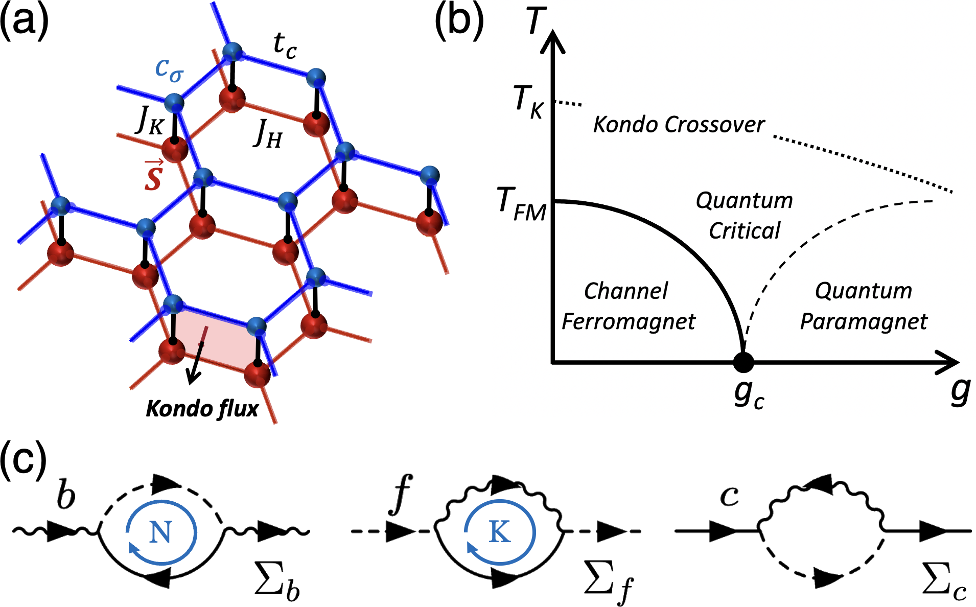
Figure 1: (a) Sketch of the honeycomb Kondo lattice studied in this paper. An example of Kondo flux, threading in between conduction electrons and Abrikosov fermions (spinons) is illustrated. (b) The phase diagram previously proposed for this system [20]. (c) Self energies for all the fields in the self-consistent equations. Each interaction vertex carries a $1/\sqrt{N}$ factor. While the internal sum over SU($N$) or SU($K$) indices brings $\Sigma_{b,f}$ to O(1), $\Sigma_{c}$ remains O$(1/N)$.

The effective theory of fluctuations was studied in [20] in the large-$N$ limit and can be stated as ${\cal L}={\cal L}_{\rm NL\sigma M}+{\cal L}_{\rm fermions}$ where

$${\cal L}_{\rm NL\sigma M}=\frac{(\partial_{\mu}\vec{n})^{2}}{g}+\Gamma(A^{\mathrm{ex}}_{\mu}-A^{f}_{\mu}-\Omega^{z}_{\mu})^{2}.$$ (2)

The first term is the usual non-linear sigma model (NL$\sigma$M) governing the fluctuations of the order parameter $\vec{n}\sim\vec{\cal O}$. At low $T$, the NL$\sigma$M has an ordered phase where channel symmetry is spontaneously broken [Fig. 1(b)], and a quantum paramagnet in which the symmetry is restored by topological defects (channel skyrmions). Here $\Omega^{z}_{\mu}$ is the gauge-dependent disorder potential, whose curl gives the the density of defects $4\epsilon^{\mu\nu\lambda}\partial_{\lambda}\Omega_{\nu}^{z}=\vec{n}\cdot(\partial_{\lambda}\times\partial_{\nu}\vec{n})$. The second term in (2) is a Higgs term which tends to lock the internal U(1) gauge field of $f$-electrons $A^{f}_{\mu}$ with the external electromagnetic gauge potential $A^{\mathrm{ex}}_{\mu}$ up to ${\Omega}^{z}_{\mu}$. In the ordered phase, defects are expelled and the internal and external gauge fields are locked, leading to a large FS, whereas in the quantum paramagnet the defects are proliferated destroying the coherent phase-locking [20, 25].

However, since the winning channel has a larger FS [26, 20] and the order parameter $\vec{\cal O}$ is strongly dissipated by coupling to fermionic degrees of freedom ${\cal L}_{\rm fermion}$, the ground state is expected to be more complicated, at least in two or three spatial dimension. This is reminiscent of of the spin-fermion model where the gapless fermionic modes need to be explicitly taken into account in the renormalization group (RG) study [27, 28, 29, 30, 31, 32, 33, 34, 35, 36, 37, 38, 39, 40, 41, 42, 43, 44].

Encouraged by recent successes of large-$N$ approach to Kondo lattices, cross-checked by tensor network [45] and Quantum Monte Carlo [46] methods, we conduct a large-$N$ study of MCKL. In a previous study [17], we applied dynamical large-$N$ approach to both 1D and $\infty$D MCKLs with Schwinger boson representation of spins and showed that spatial fluctuations are fully captured by including momentum dependence of the self-energy. In this paper, we use this technique to shed light on the issue of the symmetry breaking in the MCKL in 2+1D, i.e. between upper and lower critical dimensions.

Method — We assume the spins transform according to a fully antisymmetric representation of SU($N$) and use Abrikosov fermions $S_{{j}\alpha\beta}=f^{\dagger}_{j\alpha}f^{\vphantom{\dagger}}_{j\beta}$ with the constraint $f^{\dagger}_{j\alpha}f^{\vphantom{\dagger}}_{j\alpha}=N/2$ to form a self-conjugate representation of spins. This introduces a gauge symmetry $f_{j\alpha}\to e^{i\varphi_{j}}f_{j\alpha}$ which we track throughout the paper. We maintain the particle-hole (p-h) symmetry for both spins and conduction electrons, which means the constraint is satisfied on average. In the impurity case [47, 48] the spin is overscreened for any number of channels $K$. We rescale $J_{K}\to J_{K}/N$ and send $N,K\to\infty$ but keep their ratio $\gamma=K/N$ constant. The Lagrangian is  [49, 50]

$${\cal L}={\cal L}_{0}+\sum_{j}\left[\frac{\bar{b}_{ja}b_{ja}}{J_{K}}+\frac{1}{\sqrt{N}}(\bar{c}_{ja\alpha}f_{ja}\bar{b}_{j\alpha}+\mathrm{h.c.})\right].$$ (3)

Here, $b_{j}$ are bosonic holon fields introduced for Hubbard-Stratonovitch decoupling of the Kondo interaction. ${\cal L}_{0}$ contains the bare dispersion of conduction electrons $H_{c}(k)$ and fermionic spinons $H_{f}(k)$. The (assumed to be homogeneous) nearest-neighbor spinon hopping comes from large-$N$ decoupling of $J_{H}$. In this overscreened case, any infinitesimal $J_{H}>0$, delocalizes spinons due to resonant RKKY amplification [17]. The gauge symmetry $f_{j}\to e^{i\varphi_{j}}f_{j}$ is preserved by the Lagrangian (3), provided that $b_{j}\to e^{i\varphi_{j}}b_{j}$. The channel order parameter $\vec{\cal O}_{j}$ is equivalent to $\vec{\cal B}_{j}\equiv b^{\dagger}_{j}\vec{\tau}b^{\vphantom{\dagger}}_{j}$ as we showed before [17].

In the large-$N$ limit, we can solve the problem exactly, as the dynamics is dominated by the non-crossing Feynman diagrams [Fig. 1(c)], resulting in spinon and holon self-energies [$\vec{r}\equiv(\mathbf{r}_{j},\tau)$]

$$\Sigma_{f}(\vec{r})=-\gamma g_{c}(\vec{r})G_{b}(\vec{r}),\quad\Sigma_{b}(\vec{r})=g_{c}(-\vec{r})G_{f}(\vec{r}),$$ (4)

whereas $\Sigma_{c}$ is $\mathrm{O}(1/N)$. Hence, the electron propagator $g_{c}^{-1}(k,{\rm z})={\rm z}\mathbb{1}-{H}_{c}(k)$ remains bare, with ${\rm z}$ the complex frequency. Eqs. (4) together with the Dyson equations $G_{f}^{-1}(k,{\rm z})={\rm z}\mathbb{1}-H_{f}(k)-\Sigma_{b}(k,{\rm z})$ and $G_{b}^{-1}(k,{\rm z})=-J_{K}^{-1}\mathbb{1}-\Sigma_{b}(k,{\rm z})$ form a set of coupled integral equations that are solved iteratively and self-consistently to extract thermodynamics [51, 50]. Considering the numerical complexity of the problem, symmetries are utilized to reduce the required computation down to the fundamental domain of the Brillouin zone [52].

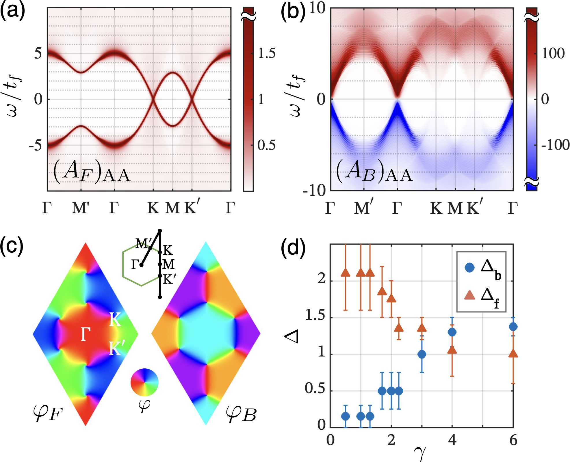
Figure 2: With only nearest-neighbor hoppings, the spectral weights of spinons and holons develops gapless lightcones displayed in (a) and (b) respectively, at a low $T$ of $T/J_{K}=0.005$, along the Brillouin zone cut shown in (c). Parameters used are $\gamma=4$, $J_{K}/t_{c}=10$, and $t_{f}/t_{c}=0.2$. (c) The phase structure in the critical eigenstates of $G_{f}^{-1}(0+i\eta,k)$ and $G_{b}^{-1}(0+i\eta,k)$, extracted from the angle $\varphi$ between the $\sigma^{x,y}$ components. The vortices and plains show a pair of critical chiral fermions at K points and an achiral boson at $\Gamma$. A $C_{3}$-symmetric reciprocal-space gauge is used instead of a periodic one. (d) Exponents of the critical solution, extracted from the $T$ scaling of spectral weight.

The 1+1D case has been studied in [17]. The ground state is a conformally invariant fixed point in which the spinons and holons have critical exponents $\Delta_{b}=\gamma/(\gamma+2)$ and $\Delta_{f}=1/2+2/(\gamma+2)$ [53, 54]. In the rest of the paper, we focus on the 2+1D MCKL on a honeycomb lattice.

For the honeycomb lattice, we defined the sublattice spinors at unit cell $j$

$$C_{ja\alpha}=\begin{pmatrix}c_{ja\alpha}^{\mathrm{A}}\\ c_{ja\alpha}^{\mathrm{B}}\end{pmatrix},\hskip 7.11317ptF_{j\alpha}=\begin{pmatrix}f_{j\alpha}^{\mathrm{A}}\\ f_{j\alpha}^{\mathrm{B}}\end{pmatrix},\hskip 7.11317ptB_{j,a}=\begin{pmatrix}b_{ja}^{\mathrm{A}}\\ b_{ja}^{\mathrm{B}}\end{pmatrix}.$$ (5)

Their conjugates are defined by $\bar{C}\equiv C^{\dagger}\sigma^{z}$, etc. Spin and channel indices will be suppressed when redundant. Furthermore, at low temperature we shall denote their low energy modes by $C\sim\psi$, $F\sim\chi$, $B\sim\phi$.

Gapless phase — First, we assume conduction electrons have only nearest-neighbor hopping as in graphene [55]. The low energy $c$-electrons are given by

$$C_{j}=e^{-i\mathbf{K}\cdot\mathbf{r}_{j}}\psi_{1}(\vec{r})+e^{-i\mathbf{K}^{\prime}\cdot\mathbf{r}_{j}}\psi_{2}(\vec{r}),$$ (6)

where $\psi_{\mu}$, $\mu=1,2$ are the chiral spinors sitting one each at the two Dirac nodes [55, 56]. We introduce three Pauli matrices $\vec{\sigma}=(\sigma^{x},\sigma^{y},\sigma^{z})$ in the sublattice space as well as the vectors $\vec{r}=(x,y,v\tau)$ and $\vec{\nabla}=(\partial_{x},\partial_{y},v^{-1}\partial_{\tau})$. This enables us to to define $\cancel{r}\equiv\vec{\sigma}\cdot\vec{r}$ and $\cancel{\partial}=\vec{\sigma}\cdot\vec{\nabla}$ for one Dirac cone, and $\bcancel{r}\equiv\vec{\sigma}^{*}\cdot\vec{r}$ and $\bcancel{\partial}=\vec{\sigma}^{*}\cdot\vec{\nabla}$ for the other with the opposite chirality. The Euclidean Lagrangian is

$${\cal L}_{0}=v_{c}\Big{(}\bar{\psi}_{1}\cancel{\partial}\psi_{1}+\bar{\psi}_{2}\bcancel{\partial}\psi_{2}\Big{)}+v_{f}\Big{(}\bar{\chi}_{1}\cancel{\partial}\chi_{1}+\bar{\chi}_{2}\bcancel{\partial}\chi_{2}\Big{)}+m_{b}\bar{\phi}\phi,$$ (7)

where $\chi_{\mu}$ denotes the spinon counterparts to $\psi_{\mu}$. In presence of the gauge field the derivatives are replaced by covariant derivatives, $D_{\psi}=\partial+A_{\rm ex}+A_{\rm ch}+A_{\rm sp}$ for electrons, and $D_{\chi}=\partial+A_{\rm in}+A_{\rm sp}$ for spinons. In addition to the SU_sp($N$) spin, SU_ch($K$) channel, U_in(1) gauge, and p-h symmetry, the low-energy action has time-reversal (TR) symmetry $i\to-i$ and inversion (I) symmetry $(x,y)\to-(x,y)$, which act on spinors according to

$${\rm TR:}\quad\begin{array}[]{cc}\psi_{1}\leftrightarrow\psi_{2}\\ \chi_{1}\leftrightarrow\chi_{2}\end{array},\qquad\text{and}\qquad{\rm I:}\quad\begin{array}[]{cc}\psi_{1}\leftrightarrow\sigma^{x}\psi_{2}\\ \chi_{1}\leftrightarrow\sigma^{x}\chi_{2}\end{array}.$$ (8)

The electron Green’s function is

$$g_{C}(\vec{r})=\frac{1}{4\pi r^{{3}}}\Big{(}e^{-i\mathbf{K}\cdot\mathbf{r}}\,{\bcancel{r}}+e^{-i\mathbf{K}^{\prime}\cdot\mathbf{r}}{\cancel{r}}\Big{)}.$$ (9)

Figures 2(a,b) show the spectral functions of spinons and holons, respectively along a cut in the reciprocal space [Fig. 2(c)]. The spectral weight of Abrikosov fermions qualitatively resembles that of a noninteracting fermion: gapless at $\mathrm{K}$ and $\mathrm{K}^{\prime}$ with opposite phase windings shown in Fig. 2(c). Furthermore, its bandwidth is resonantly amplified, similar to that of Schwinger bosons [17].

However, there is a crucial difference, namely the strong incoherent contribution inside the light cones. In fact, this interaction-driven fixed point exhibits a 2+1D criticality, which leads to power-law spectrum at low frequencies. We find that Green’s functions are in good agreement with the conformally invariant ansatzes

$$G_{F}(\vec{r}) = \frac{\alpha_{f}}{4\pi r^{{2\Delta_{f}+1}}}\Big{(}e^{-i\mathbf{K}\cdot\mathbf{r}}{\bcancel{r}}+e^{-i\mathbf{K}^{\prime}\cdot\mathbf{r}}{\cancel{r}}\Big{)}$$

$$G_{B}(\vec{r}) = \frac{\alpha_{b}}{4\pi r^{{2\Delta_{b}}}}{\cal P}_{b},$$ (10)

where ${\cal P}_{b}=\frac{1}{2}(1+\sigma^{x})$ is a projector to the molecular bonding state between A and B sublattices. This is consistent with the observation that only uniform (rather than staggered) channel susceptibility diverges at low $T$. So, the low energy spinor for the holon is $\phi\equiv\mathcal{P}_{b}B$.

We have used scaling analysis [54] to extract critical exponents $\Delta_{f}$ and $\Delta_{b}$ as shown in Fig. 2(d). To summarize, the ground state of the model is governed by a conformally invariant fixed point ${\cal L}_{*}$ which preserves the channel symmetry. This is true for any $J_{K}$, in marked contrast to mean-field theory and single-site DMFT. Symmetry breaking can be induced, but does not happen spontaneously here, as was the case in [17].

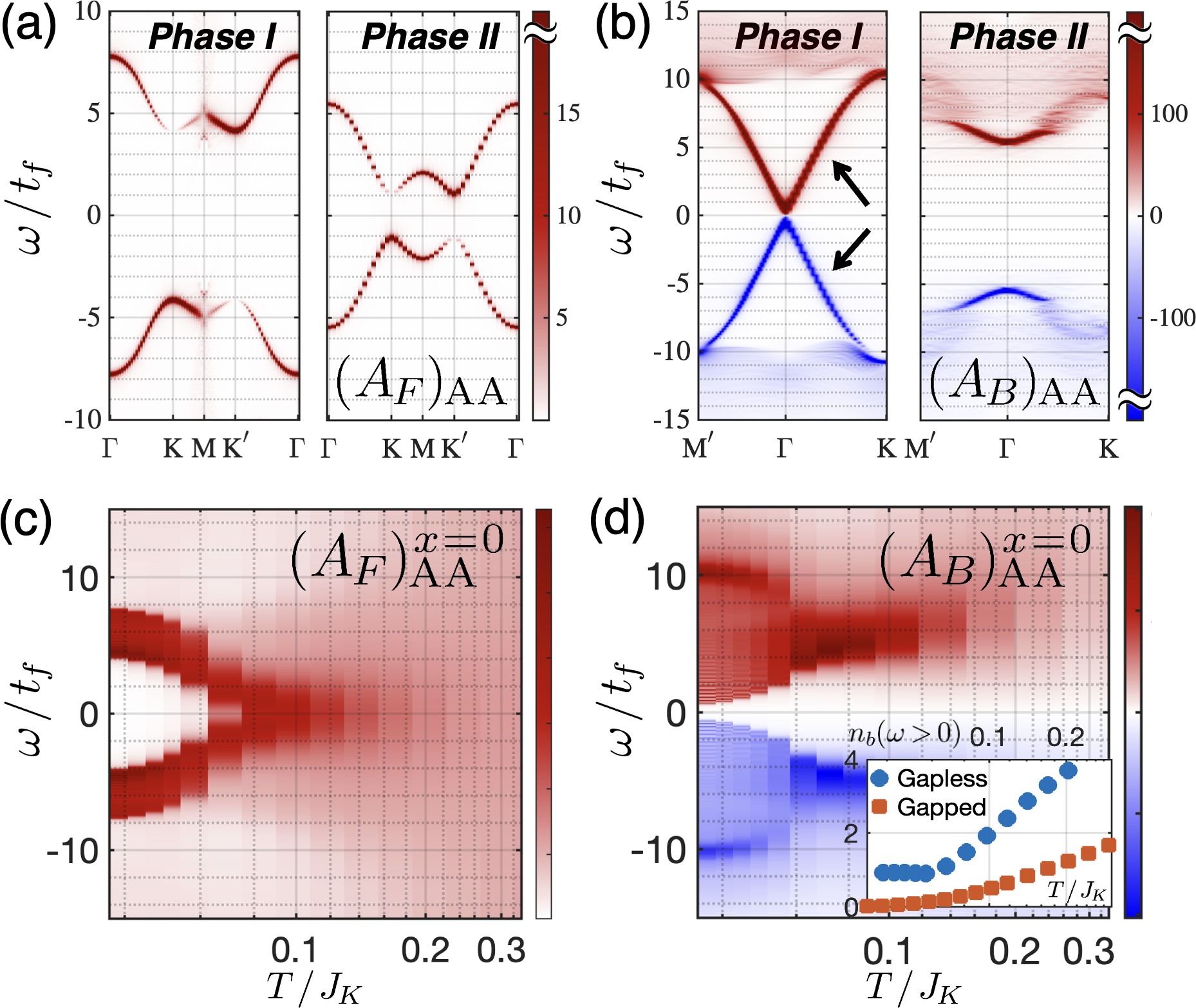
Figure 3: (a–b) Low $T$ spectral weights of (a) spinons and (b) holons in the presence of topologically nontrivial conduction channels, both in (I) the channel symmetry-broken phase and (II) the channel symmetric phase, at $T/J_{K}=0.03$. The arrows point to a true p-h symmetric bound-state $\phi\sim\psi\chi$ and $\phi^{\dagger}\sim\psi^{\dagger}\chi^{\dagger}$ in an otherwise gapped spectrum. (c–d) Temperature evolution of the local spectral weights in Phase I, of (c) spinons and (d) holons. Inset of (d) shows the population of free holons, which become conserved at low $T$s. Parameters used are $J_{K}/t_{c}=6$, $|t_{c}^{\prime}/t_{c}|=0.5$, and $|t_{f}/t_{c}|=0.2$. Phase I data is at $\gamma=1$, and Phase II at $\gamma=5$.

Gapped phase — Next we break the TR symmetry [57] by including magnetic fluxes only in the conduction electron layer, while preserving a zero net flux per plaquette. This opens a gap in the conduction electron spectrum. Remarkably, the $f$-spinons inherit a similar gap via the phenomenon of resonantly enhanced dispersion we reported before [17] [Fig. 1(a)]. The form and the nature of the gap, however, depends on the parameter $\gamma=K/N$ and various distinct phases are discernible. At large $\gamma>2$ we find that fermionic spinons and bosonic holons are both gapped and the spectra are independent of temperature at low $T$, as shown in Phase II of Fig. 3(a,b). At smaller $\gamma<2$ (Phases I) we find that fermions have a different shape of dispersion and bosons have a spectral gap that depends on $T$. Figures 3(c,d) show the temperature evolution of the spectral gap for spinons and holons. As the $T$ is lowered, a gap opens in the local spectrum of spinons. However, the gap in the spectrum of bosons collapse by reducing $T$, so that at the $T\to 0$ ground state, the bosons are gapless.

The qualitative picture presented above, persists for small TR-breaking gap. Therefore, a renormalization group (RG) discussion of the nature of these massive phases is in order. For $\gamma>2$, the critical exponents [Fig. 2(d)] indicate that $\Delta_{f}<3/2$. This means that a mass term of the form ${\cal L}={\cal L}_{*}+m_{f}(\bar{\chi}_{1}\chi_{1}-\bar{\chi}_{2}\chi_{2})$ is a relevant perturbation, in an RG sense. Note that a Semenoff mass [58] is forbidden due to the assumed inversion symmetry. Indeed in Phase II, $\left\langle\bar{\chi}_{1}\chi_{1}-\bar{\chi}_{2}\chi_{2}\right\rangle\neq 0$. The mass has different signs at the two K points, which can be attributed to the Kondo-flux repulsion [Fig. 1(a)]. As seen in Fig. 2(d), $\Delta_{f}=1$ and the bulk fermion is a usual non-interacting 2D topological insulator. This characterizes a chiral spin-liquid in which the TR-breaking is induced on spinons via the Kondo interaction.

For $\gamma<2$ such mass term is irrelevant and the origin of the spinon gap is more subtle. The only relevant interaction in this case, is ${\cal L}={\cal L}_{*}+[V_{a}(\psi_{1,a\alpha}^{\dagger}{\cal P}_{b}\chi_{1,\alpha}^{\vphantom{\dagger}}+\psi_{2,a\alpha}^{\dagger}{\cal P}_{b}\chi_{2,\alpha}^{\vphantom{\dagger}})+\mathrm{h.c.}]$ with a c-number $V_{a}$ which is relevant for all $\gamma$. Indeed, the spinon dispersion in Phase I can be fitted with a hybridization model between bare $c$ and $f$-electrons [54], whereas the TR-broken Haldane model is sufficient for Phase II. However, such a mass-term is forbidden not only due SU($K$) channel symmetry, but also the U(1) gauge symmetry $\chi\to e^{i\varphi}\chi$ of the Lagrangian. Such mass generation has been discussed in the context of of symmetric mass generation [59, 60, 61] where a finite $\|V\|$ is maintained but the direction of $V$ spinor is randomized. Since gauge fields are involved, what we have here is rather dynamic mass generation (DMG) [62, 63, 64] which creates a massive particle with conserved particle number (see below) below a critical number of flavors.

In 2+1D, abelian gauge fields coupled to many flavors of fermions are screened and are in the deconfining phase [62]. For non-abelian gauge fields coupled to $N_{f}$ flavor of fermions with $N_{c}$ colors, in the limit of $N_{f}\gg N_{c}$, self-interactions are negligible and they behave like abelian fields, i.e. are in the deconfining phase. On the other hand, in the limit of $N_{c}\gg N_{f}$ self-interactions are important and the gauge fields essentially behave as free Yang-Mills which are confining [62]. Since they are coupled to fermions, for $N_{c}\gg N_{f}$ there is a tendency to dynamically generate a mass. The critical number of flavors is predicted to be at $\gamma_{c}=N_{f}/N_{c}\to 64/3\pi^{2}\approx 2.16$.

From this discussion, we see that the U_in(1) gauge field coupled to $N$ fermions is always deconfining. But it can also be Higgsed if the bosons, also carrying U_in(1) charge, condense (see below). The SU_sp($N$) gauge field has $N$ colors and $K$ flavors and is in the deconfining phase for $\gamma>\gamma_{c}$. On the other hand for $\gamma<\gamma_{c}$ it is confining and therefore electrons and spinons, which carry corresponding charges, are confined into a bosonic bound-state. The role of color and flavor changes for the SU_ch($K$) gauge field. This one is expected to be confining at $\gamma>\gamma^{\prime}_{c}$ so that the holons are glued to the electrons. This essentially means the free spinons are Kondo coupled to electrons and the Kondo interaction cannot be decoupled in this limit. For $\gamma<\gamma^{\prime}_{c}$ the holons and bound-states are deconfined and free to condense. For $\gamma^{\prime}_{c}<\gamma<\gamma_{c}$ electron-spinon bound states have formed, but since they carry channel quantum number, they are confined due to SU_ch($K$) fluctuations. From our numerics we find $\gamma^{\prime}_{c}\sim 1$ rather than 0.426 predicted by the fully symmetric model.

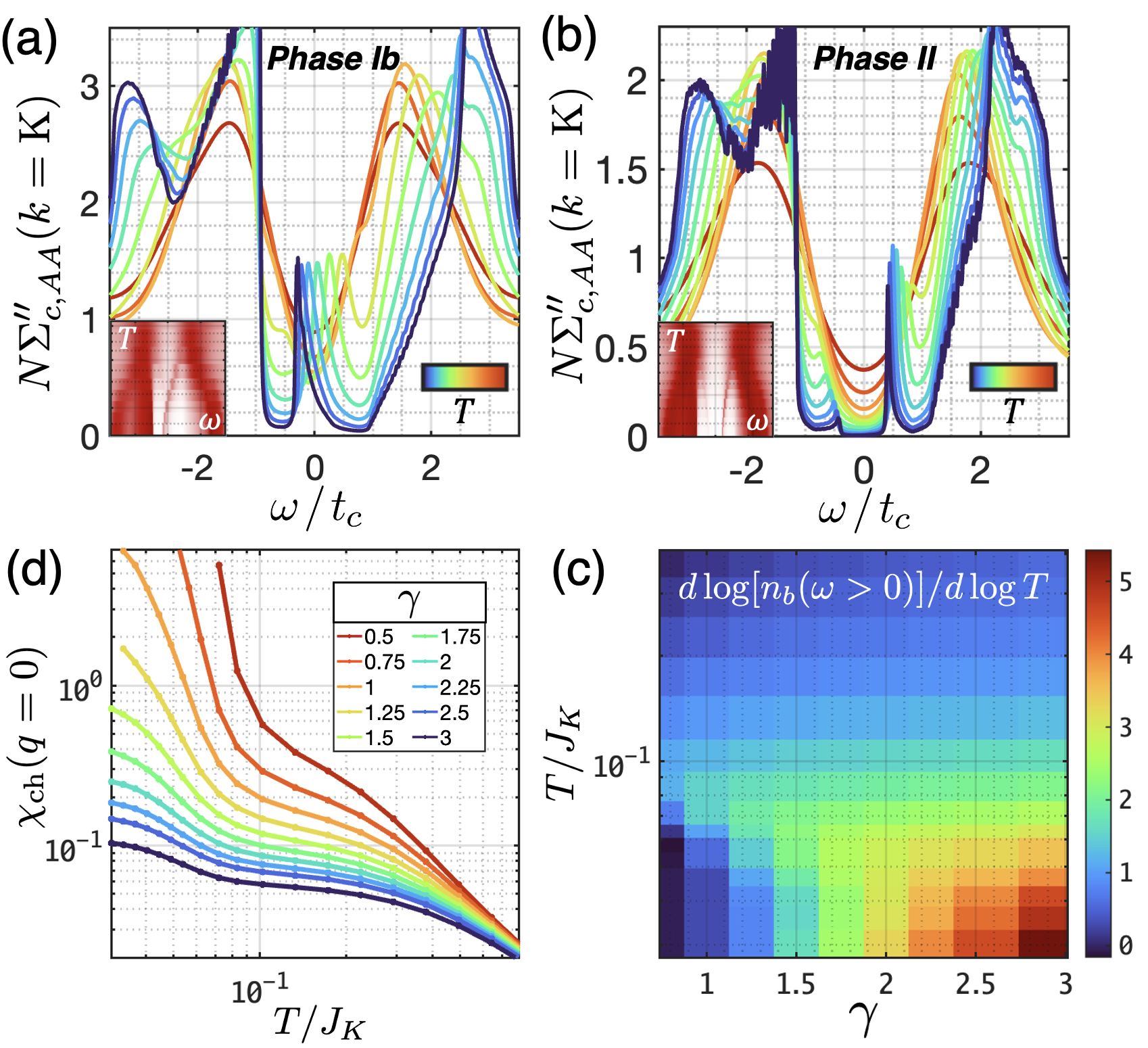
Figure 4: (a-b) The spectrum of the self-energy of conduction electrons in Phases Ib and II. Whereas a gap is present in Phase II, a resonance crosses zero energy in Phase Ib. (c) Positive occupation of bosons, represented by $\xi(T)\equiv\mathrm{d}\log n_{b}(\omega>0)/\mathrm{d}\log T$. At low $T$, $\xi(T)$ vanishes in Phase Ia, diverges in Phase II and is a constant in Phase Ib, reflecting $n_{b}(\omega>0)\sim T^{\xi}$. (d) Uniform channel susceptibility $\chi_{\mathrm{ch}}(q=0)$ vs. $T$ at several $\gamma$, at a fixed $t_{f}=0.4t_{c}$, i.e., fixed $J_{H}$ at low $T$. Low temperature $\chi_{\mathrm{ch}}$ diverges in Phase Ia, signaling spontaneous channel symmetry breaking and the formation of a channel ferromagnet.

The spectrum of bosons in Phase I of Fig. 3(b) contains a sharp and fully coherent resonance [pole of $G_{B}(k,{\rm z})$] at lowest energy which can be attributed to a bound-state $\phi_{a}\sim\psi^{\dagger}_{a\alpha}\chi^{\vphantom{\dagger}}_{\alpha}$ between conduction electrons and spinons. The bound state is described by ${\cal L}_{\phi}\sim\bar{\phi}[\nabla^{2}+m^{2}(T)]\phi$, with a mass which approaches zero $m(T\to 0)=0$. This is manifested as a pole in the conduction electron self-energy $N\Sigma_{c}({\rm k},{\rm z})$ at $k=$K, K^′ that crosses zero energy for $\gamma<2$, whereas $N\Sigma_{c}(k,{\rm z})$ remains gapped in Phase II [Fig. 4(c,d)]. The significance of the pole is that it leads to an enlargement of the conduction electron FS in Phase I. Note that no such pole exists in the gapless TR-preserving phase [65], but a heavily damped pole cannot be rule out in that case.

Can the bosonic gap closing lead to channel symmetry breaking? Since bosons are the byproduct of the Hubbard-Stratonovitch decoupling of the Kondo interaction, they do not condense as there are no conservation of boson numbers. A closer look at how the boson gap closes, reveals that the behavior of gapless bosons change within Phase I. For $\gamma<1$ (Phase Ia), the positive frequency population of bosons $n_{b}(\omega>0)\equiv\int_{0}^{\infty}{\frac{\mathrm{d}\omega}{2\pi}}{n(\omega){\rm Tr}A_{B}(\omega-i\eta)}$ stays constant with temperature, whereas for $1<\gamma<2$, (Phase Ib) this positive frequency population decays to zero as a power-law $n_{b}(\omega>0)\sim T^{\xi}$. These two behaviors are shown in the inset of Fig. 3(d), as well as colormap of Fig. 4(c) and are in marked contrast to the exponential decay in Phase II, $n_{b}(\omega>0)\sim e^{-m_{b}/T}$. Therefore, there is an emergent conservation of boson number in Phase Ia, which was certainly absent at the UV. At $T=0$, conserved bound-states reach zero energy and condense in one of the channels $a$, equivalent to spontaneous breaking of the channel symmetry. This is reflected in the divergence of uniform channel susceptibility $\chi_{\mathrm{ch}}(q=0)$, shown in Fig. 4(d). For $\gamma<1$, $\chi_{\mathrm{ch}}(q=0)$ diverges at low $T$, whereas it saturates at $\gamma>1$. The transition is also seen by varying $J_{H}$ [54].

The transition between Phase Ia and Ib is reminiscent of the phase diagram of the NL$\sigma$M, describing a channel ferromagnet and a quantum paramagnet and the destruction of order by topological defects. The paramagnet is a channel spin liquid, since local moments are screened, and does not have any local order parameter. The agreement with Fig. 1(b) is not surprising, as in presence of the gap, fermions can be safely integrated out and the effective interaction of Eq. (2) is expected be valid. These phases are summarized in the phase diagram of Fig. 5.

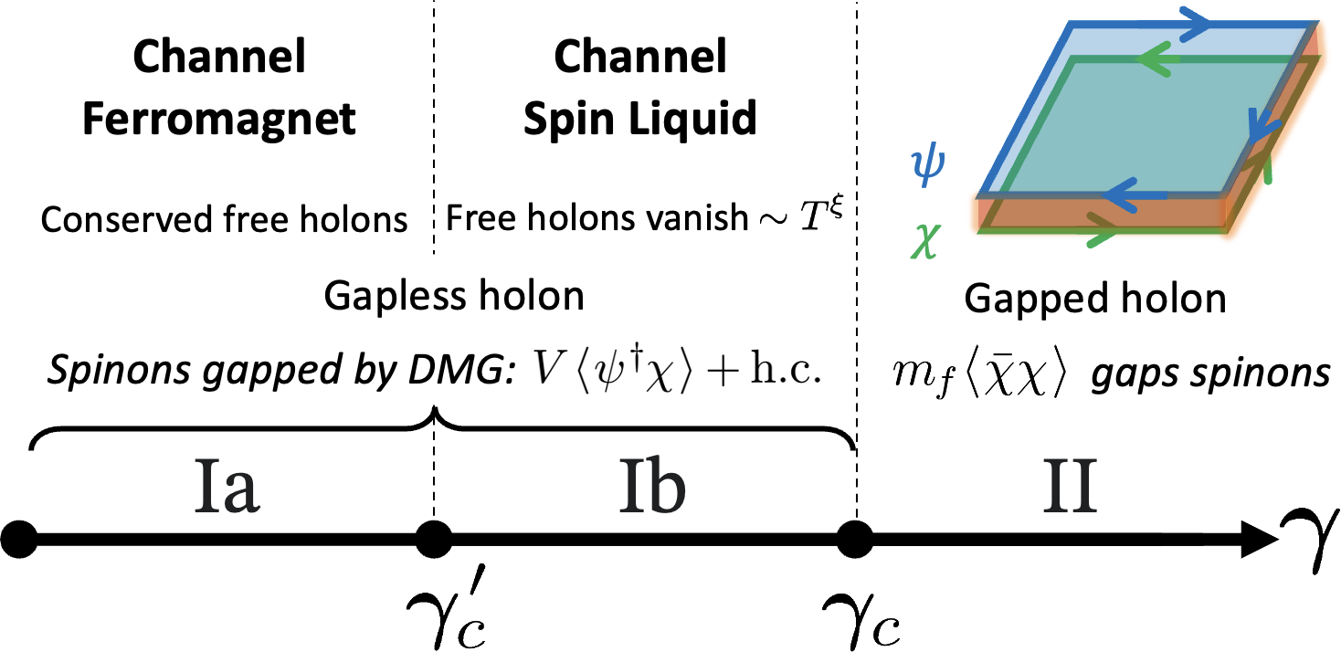
Figure 5: Phase diagram in the presence of a Haldane mass on $c$-electrons, as a function of channel number $\gamma=K/N$. The three phases have distinct behaviors of $\chi_{\mathrm{ch}}(T)$, electron self-energy and free holon population. We argue that the Phase I has dynamic mass generation (DMG) and by itself is divided into a channel ferromagnet and a quantum paramagnet, whereas Phase II is a fractional Chern insulator (FCI). Our numerical results suggest $\gamma_{c}\sim 2$ and $\gamma^{\prime}_{c}\sim 1$.

In the entire Phase I, the hybridization is active, the local moments are screened and the resonance in self-energy $\Sigma_{c}$ suggests a large FS. However, while the $f$-electrons respond coherently to the external field due to the locking between $A^{\rm in}$ and $A^{\rm ex}$ in the ordered Phase Ia, this coherence is lost in the disordered Phase Ib. According to Oshikawa’s theorem [66], the small-FS Fermi liquid in the otherwise gapped Phase 2 is only possible in presence of a topological order [14].

The topological gap in Phase II leads to edge modes composed of counter-propagating electrons $c$ and non-interacting spinons $f$, on an open manifold. These two gapless modes are still coupled via the Kondo interaction $J_{K}\vec{\cal J}^{R}\cdot\vec{\cal S}^{L}$ where ${\cal J}^{R}_{\alpha\beta}=c^{\dagger}_{a\alpha}c^{\vphantom{\dagger}}_{b\beta}$ and ${\cal S}^{L}_{\alpha\beta}=f^{\dagger}_{\alpha}f^{\vphantom{\dagger}}_{\beta}$ are SU_K($N$) and SU₁($N$) Kac-Moody currents, respectively. The interaction is marginally relevant and lowers the central charge of the $f$ edge modes from ${\rm c}_{\rm UV}/N=1$, due to the c-theorem [67]. In fact, this chiral model is one half of the 1D 2CKL model studied by Andrei and Orignac [68, 69, 70]. Generalizing their SU_sp(2)$\times$ SU_ch($K$) model to the present SU_sp($N$)$\times$ SU_ch($K$) symmetry group, it is natural to expect that the IR edge mode is governed by the chirally-stabilized [71] fixed point

$${\cal L}_{\text{Phase II}}\to{\rm SU}_{K-1}{\rm(}N{\rm)}\times\frac{{\rm SU}_{K-1}{\rm(}N{\rm)}\otimes{\rm SU}_{1}{(\rm}N{\rm)}}{{\rm SU}_{K}{\rm(}N{\rm)}},$$ (11)

in addition to the decoupled charge and channel sectors [17]. This means that Phase II realizes a fractional Chern insulator (FCI) [72, 73], whose edge mode is comprised of an electron, an SU_K-1($N$) mode, as well as another anyonic mode from the coset sector. In the large-$N$ limit, this theory leads to a central charge of $\lim_{N\to\infty}{\rm c}_{N}(\gamma)/N=\gamma/(1+\gamma)$ in addition to fully decoupled conduction electrons [17]. From bulk-boundary correspondence we expect the bulk to have similar fractionalized description in terms of the gauged Chern-Simons theory. A detailed computation of electric and thermal Hall conductivities and investigation of other properties of FCI [74], as well as connections to the order fractionalization [26, 75] are beyond scope of the present work and will be reported elsewhere.

In conclusion, by including spatial fluctuations in a multichannel Kondo lattice in two spatial dimensions, we have shown that the channel symmetry is preserved as opposed to single-site DMFT and static mean-field calculations. The phase diagram Fig. 1(b) of NL$\sigma$M does not apply to a Kondo lattice below upper critical dimension, as the gapless fermions drive the system toward a conformally invariant fixed point. We have characterized this fixed point in the large-$N$ limit by finding the critical exponents using a scaling ansatz. Breaking time-reversal symmetry by adding a Haldane mass to the conduction electrons, gaps out spinons and holons by resonant RKKY amplification. In this case, however, we recover the phase diagram of Fig. 1(b) where in one phase both spinons and holons are gapped whereas in the other, an emergent stabilization of holon population and a temperature dependence of the gap, indicate a gapless groundstate for the holons and a spontaneous breaking of the channel symmetry similar to the NL$\sigma$M description. We have discussed the role of gauge fields and argued that the gapped phase realizes a fractional Chern insulator, with the edge modes given by the theory of [68].

The 2CKL of common spins fall at the border between Phases Ia and Ib, but the validity of our large-$N$ results for $N=2$, remains to be explored.

It is a pleasure to acknowledge fruitful discussions with N. Andrei, P. Coleman and R. Wijewardhana. This work was performed in part at Aspen Center for Physics, which is supported by NSF Grant No. PHY-1607611. Computations for this research were performed on the Advanced Research Computing Cluster at the University of Cincinnati, and the Ohio Supercomputer Center.

Appendix A Supplementary materials

A.1 A. Duality between Abrikosov fermion and Schwinger boson representations in Kondo lattices

In the dynamical large-$N$ method, the low energy effective theory of the overscreened Kondo lattices derived from the self-consistent equations using the Abrikosov fermion and Schwinger boson representation of the spins are dual to each other. In the latter case, the spinons are Schwinger bosons, also denoted by $b$, and the holons are fermionic fields $\chi$ [50, 17]. The duality is

$$f\leftrightarrow\chi,\quad b\leftrightarrow b,\quad\gamma\leftrightarrow 1/\gamma.$$ (12)

The scaling exponents for the 1+1D Kondo lattice using the Abrikosov fermion representation is plotted in Fig. 6. It agrees with the exponents reported in Ref. 17 by duality.

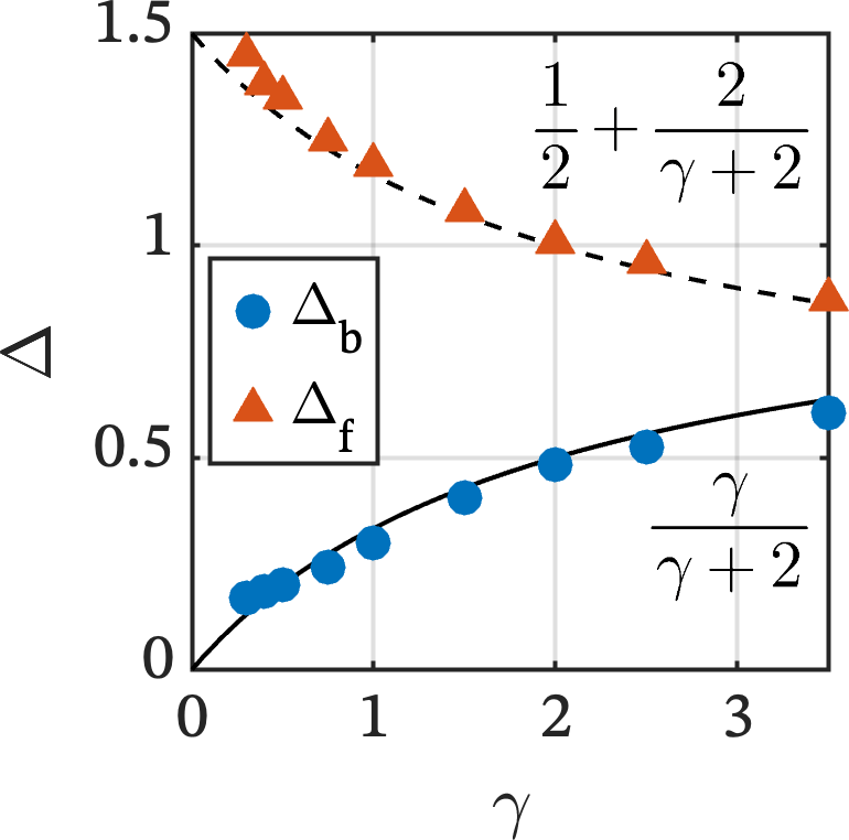
Figure 6: Scaling exponents for the 1+1D overscreened Kondo lattice using large-$N$ Abrikosov fermion self-conjugate representation. The curves are conformal solution exponents.

A.2 B. Numerical method for the dynamical large-$N$ equations

The Dyson equations for spinons and holons together with the self energies equations in Eqs. (4) constitute a set of self-consistent equations. In the present case of the Kondo lattice with the large-$N$ Abrikosov fermion representation of the spins, they are numerically solved to $\mathrm{O}(1)$ by essentially the same method applied to the Schwinger boson representations in Ref. 17. We derive the details of self-consistent equations below.

The self energies for a lattice displacement-imaginary time $\vec{r}=(i,j,\tau)$ are

$$\left[\Sigma_{F}(\vec{r})\right]_{\kappa\lambda} = -\gamma[g_{C}(\vec{r})]_{\kappa\lambda}[G_{B}(\vec{r})]_{\kappa\lambda},$$ (13)

$$\left[\Sigma_{B}(\vec{r})\right]_{\kappa\lambda} = [g_{C}(-\vec{r})]_{\lambda\kappa}[G_{F}(\vec{r})]_{\kappa\lambda},$$ (14)

$$N\left[\Sigma_{C}(\vec{r})\right]_{\kappa\lambda} = -[G_{B}(-\vec{r})]_{\lambda\kappa}[G_{F}(\vec{r})]_{\kappa\lambda},$$ (15)

where $\kappa$ and $\lambda$ denote sublattice indices. Note the sublattice transpose for backward propagation ($-\vec{r}$). We solve this system of equations using spectral functions of the Green’s functions and self energies in real frequency-momentum space, with $\Sigma_{C}$ dropped at $\mathrm{O}(1)$. The self energies may be obtained from Hilbert transforms of $A_{\Sigma}(\omega)\coloneqq i\Sigma(\omega+i\eta)-i\Sigma(\omega-i\eta)$, where $\eta\to 0^{+}$. They are given by

$$\left[{A_{\Sigma}}_{F}(\mathbf{k},\omega)\right]_{\kappa\lambda} = -\frac{\gamma}{\mathcal{V}}\sum_{\mathbf{p}}\int\frac{\mathrm{d}\nu}{2\pi}[A_{C}(\mathbf{p},\nu)]_{\kappa\lambda}[A_{B}(\mathbf{k}-\mathbf{p},\omega-\nu)]_{\kappa\lambda}[f(\nu)+n_{B}(\nu-\omega)],$$ (16)

$$\left[{A_{\Sigma}}_{B}(\mathbf{k},\omega)\right]_{\kappa\lambda} = \frac{1}{\mathcal{V}}\sum_{\mathbf{p}}\int\frac{\mathrm{d}\nu}{2\pi}[A_{C}(\mathbf{p},\nu)]_{\lambda\kappa}[A_{F}(\mathbf{k}+\mathbf{p},\omega+\nu)]_{\kappa\lambda}[f(\nu)-f(\omega+\nu)],$$ (17)

where $f$ and $n_{B}$ are respectively Fermi-Dirac and Bose-Einstein distributions, and $\mathcal{V}$ is the system size. Since $c$-electrons remain bare at $\mathrm{O}(1)$, we can use the explicit form of $A_{C}$. Denote the Pauli matrices by $\vec{\sigma}\coloneqq(\sigma^{x},\sigma^{y},\sigma^{z})$. For $H_{c}(\mathbf{k})=\vec{\epsilon}_{\mathbf{k}}\cdot\vec{\sigma}-\mu_{\mathbf{k}}\mathbb{1}$. $g_{C}^{-1}(\mathbf{k},\mathrm{z})=(\mathrm{z}+\mu_{\mathbf{k}})\mathbb{1}-\vec{\epsilon}_{\mathbf{k}}\cdot\vec{\sigma}$. When $\epsilon_{\mathbf{k}}\coloneqq\|\epsilon_{\mathbf{k}}\|\neq 0$, the spectral function of $c$-electron is

$$A_{C}(\mathbf{k},\omega)=\pi\left[\left(\mathbb{1}+\frac{\vec{\epsilon}_{\mathbf{k}}\cdot\vec{\sigma}}{\epsilon_{\mathbf{k}}}\right)\delta(\omega+\mu_{\mathbf{k}}-\epsilon_{\mathbf{k}})+\left(\mathbb{1}-\frac{\vec{\epsilon}_{\mathbf{k}}\cdot\vec{\sigma}}{\epsilon_{\mathbf{k}}}\right)\delta(\omega+\mu_{\mathbf{k}}+\epsilon_{\mathbf{k}})\right].$$ (18)

When $\epsilon_{\mathbf{k}}=0$, it reduces to $A_{C}(\mathbf{k},\omega)=2\pi\delta(\omega+\mu_{\mathbf{k}})\mathbb{1}$. Substituting $A_{C}$ into Eqs.(16) and (17) gives

$$\left[{A_{\Sigma}}_{F}(\mathbf{k},\omega)\right]_{\kappa\lambda} = -\frac{\gamma}{2\mathcal{V}}\sum_{\mathbf{p}}\sum_{s=\pm}\left[\mathbb{1}+\frac{\vec{\epsilon}_{\mathbf{p}}\cdot\vec{\sigma}}{s\epsilon_{\mathbf{p}}}\right]_{\kappa\lambda}[A_{B}(\mathbf{k}-\mathbf{p},\omega-s\epsilon_{\mathbf{p}})]_{\kappa\lambda}[f(s\epsilon_{\mathbf{p}})+n_{B}(s\epsilon_{\mathbf{p}}-\omega)],$$ (19)

$$\left[{A_{\Sigma}}_{B}(\mathbf{k},\omega)\right]_{\kappa\lambda} = \frac{1}{2\mathcal{V}}\sum_{\mathbf{p}}\sum_{s=\pm}\left[\mathbb{1}+\frac{\vec{\epsilon}_{\mathbf{p}}\cdot\vec{\sigma}}{s\epsilon_{\mathbf{p}}}\right]_{\lambda\kappa}[A_{F}(\mathbf{k}+\mathbf{p},\omega+s\epsilon_{\mathbf{p}})]_{\kappa\lambda}[f(s\epsilon_{\mathbf{p}})-f(\omega+s\epsilon_{\mathbf{p}})].$$ (20)

The retarded or advanced self energies are obtained from $A_{\Sigma}$’s with a Hilbert transform, $\Sigma(\omega\pm i\eta)=-\frac{1}{2}\mathfrak{H}[A_{\Sigma}](\omega)\mp\frac{i}{2}A_{\Sigma}(\omega)$. Next we need the Dyson equations

$$G_{F}^{-1}(\mathbf{k},{\rm z}) = {\rm z}\mathbb{1}+{\mu}_{F}-H_{F}(\mathbf{k})-\Sigma_{F}(\mathbf{k},{\rm z}),$$ (21)

$$G_{B}{-1}(\mathbf{k},{\rm z}) = -J_{K}^{-1}-\Sigma_{B}(\mathbf{k},{\rm z}).$$ (22)

Here $\mu_{F}$ and $J_{K}$ are diagonal in sublattice basis but may not be proportional to $\mathbb{1}$ when, e.g., inversion symmetry is broken.

The system is solved by iterating through Eqs. (19)–(22). At the end of each iteration, one need to adjust $\mu_{f}$ to satisfy the constraint $2S/N=\langle f^{\dagger}f\rangle$ on both sublattices. As outlined in Ref. 17, we start at a high temperature, where we run the self-consistency iterations until $G$’s converge, and then lower the temperature and repeat.

The constraint simplifies when the entire system has particle-hole (p-h) symmetry on all sublattice sites. This occurs when the spin size is $S/N=1/2$, while $H_{c}$ and $H_{f}$ have p-h and inversion symmetries. Then $\mu_{f}=\mu_{c}=0$ always. We will use this condition unless otherwise specified.

Note that similar to the case with Schwinger bosons [17], the diagonal part of the holon Green’s function $G_{B}(\omega\pm i\eta)_{\kappa\kappa}$ is not strictly casual, i.e., $[G_{B}(\omega\pm i\eta)]_{\kappa\kappa}+1/2\{\mathfrak{H}[A_{B}](\omega)\pm iA_{B}(\omega)\}_{\kappa\kappa}=-J_{K}\neq 0$, and neither is $\Sigma_{F}$. However, the difference is always a real constant. It will be automatically absorbed in $\mu_{F}$ when applying the constraint on $G_{F}$.

A.3 C. Simplifying numerics with symmetries

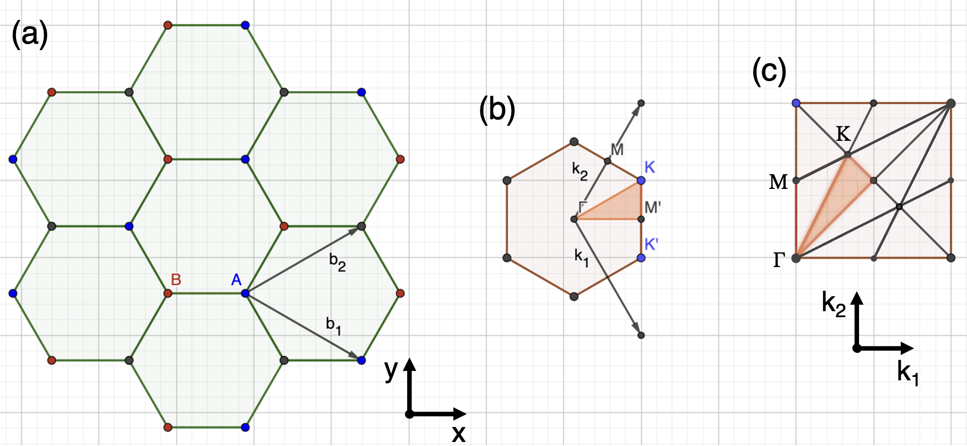
Figure 7: (a) Honeycomb lattice with the unit cell sublattice labeled AB. (b) First Brillouin zone in the $(k_{x},k_{y})$ coordinate. The reciprocal Bravais vectors $\mathbf{k}_{1}$ and $\mathbf{k}_{2}$ are shown. The fundamental domain is the highlighted orange triangle. (c) First Brillouin zone in the $(k_{1},k_{2})$ coordinate, divided into the 12 images of the fundamental domain.

Table 1: Momentum space maps and sublattice-basis representations of the crystalline symmetries of the honeycomb lattice, and of some internal symmetries: time-reversal $\mathcal{T}$, sublattice $\mathcal{S}$, and p-h $\mathcal{C}$. Their maps $R:(q_{1},q_{2})\to(q_{1}^{\prime},q_{2}^{\prime})$ are given in the reciprocal Bravais vector coordinate. Their unitary representations $U^{\prime}_{R}$ in the sublattice basis are given in the $C_{3}$-invariant Bloch basis gauge choice. These symmetries does not act on spins.

	$C_{3}$	$C_{2}$	$C_{6}$	$M_{x}$	$M_{y}$	$\mathcal{T}$	$\mathcal{S}$	$\mathcal{C}$
$R$	$(-q_{2},q_{1}-q_{2})$	$(-q_{1},-q_{2})$	$(q_{1}-q_{2},q_{1})$	$(q_{2},q_{1})$	$(-q_{2},-q_{1})$	$(-q_{1},-q_{2})$	$(q_{1},q_{2})$	$(-q_{1},-q_{2})$
$U^{\prime}_{R}$	$\mathbb{1}$	$\sigma^{x}$	$\sigma^{x}$	$\mathbb{1}$	$\sigma^{x}$	$\mathcal{K}$	$\sigma^{z}$	$\sigma^{z}\mathcal{K}$

A full calculation throughout the first Brillouin zone (1BZ) is computationally expensive. We compute only $\mathbf{k}$-points in the fundamental domain of our Lagrangian on the 1BZ [52]. In particular, with full crystalline symmetries of the honeycomb lattice $C_{6v}$, the number of $\mathbf{k}$-points needed is reduced by a factor of 12 in large systems. In the following we discuss this procedure in detail. Note that we further reduced computation load utilizing the p-h symmetry and any remaining degeneracies for Eqs. (19)–(20).

The honeycomb lattice and its 1BZ is show in Fig. 7, with unit cell defined by a pair of AB sublattice sites along $x$, separated by $\mathbf{a}_{0}\coloneqq\overrightarrow{\mathrm{AB}}$. Before writing down the symmetry operators we need to pick the gauge(s) for the Bloch basis we use. The gauge most friendly to the self-consistent equations is the reciprocal-lattice periodic gauge,

$$\left(\left|u_{\mathbf{k}}\right\rangle_{\mathrm{A}},\left|u_{\mathbf{k}}\right\rangle_{\mathrm{B}}\right)=\frac{1}{\sqrt{\mathcal{V}}}\sum_{\mathbf{k}}e^{-i\mathbf{k}\cdot\mathbf{r}_{j}}\left(\left|u_{j}\right\rangle_{\mathrm{A}},\left|u_{j}\right\rangle_{\mathrm{B}}\right).$$ (23)

Other gauges may require a twist at the boundary of 1BZ in the sums of Eqs. (19)–(20). Friendly to our symmetry discussion is another gauge choice,

$$\left(\left|u^{\prime}_{\mathbf{k}}\right\rangle_{\mathrm{A}},\left|u^{\prime}_{\mathbf{k}}\right\rangle_{\mathrm{B}}\right)=\frac{1}{\sqrt{\mathcal{V}}}\sum_{\mathbf{k}}e^{-i\mathbf{k}\cdot\mathbf{r}_{j}}\left(\left|u_{j}\right\rangle_{\mathrm{A}},e^{-i\mathbf{k}\cdot\mathbf{a}_{0}}\left|u_{j}\right\rangle_{\mathrm{B}}\right).$$ (24)

We will refer to it as the $C_{3}$-invariant gauge, and denote it by the prime. Hamiltonians and one-particle Green’s functions in these two gauges are related by the gauge transformation $\Lambda(\mathbf{k})$, expressed below in the $(k_{1},k_{2})$ coordinate shown in Fig. 7(c), where $b$ is lattice spacing.

$$[G,H](\mathbf{k}) = \Lambda(\mathbf{k})[G^{\prime},H^{\prime}](\mathbf{k})\Lambda^{{\dagger}}(\mathbf{k})$$ (25)

$$\Lambda(\mathbf{k}) = \begin{pmatrix}1&\\ &e^{i\mathbf{k}\cdot\mathbf{a}_{0}}\end{pmatrix}=\begin{pmatrix}1&\\ &e^{-i(k_{1}+k_{2})b/3}\end{pmatrix}.$$ (26)

A symmetry operation $R$ is represented in reciprocal space by unitary transformations and $\mathbf{k}$-mappings, $U^{\prime}_{R}(\mathbf{k})H^{\prime}(\mathbf{k})U^{\prime\dagger}_{R}(\mathbf{k})=H^{\prime}(R\mathbf{k})$. The $C_{6v}$ group of the lattice has rotation symmetries $C_{2}$, $C_{3}$ and $C_{6}$, as well as in-plane reflection symmetries $M_{x}$ and $M_{y}$. They are listed in Table. 1 along with the internal symmetries. Note that the time-reveral symmetry $\mathcal{T}$ we use here does not act in the spin space. To convert back to the periodic gauge, we use

$$U_{R}(\mathbf{k})=\Lambda(R\mathbf{k})U_{R}^{\prime}(\mathbf{k})\Lambda^{{\dagger}}(\mathbf{k}).$$ (27)

For example, in the periodic gauge $C_{3}\circeq\begin{pmatrix}1&\\ &e^{ik_{2}b}\end{pmatrix}$, $b$ the length of a real space Bravais vector.

The action or Hamiltonian may break some of the bare lattice symmetries. Accordingly, we pick different set of generators for different cases we study.

1. In the simplest case, when the Hamiltonian has only real NN hopping, Kondo interaction and uniform chemical potentials, we pick $\{C_{3},C_{2},M_{x}\}$ as generators.

2. In the presence of complex next-nearest-neighbor hopping giving rise to the Haldane mass, $M_{x}$, $M_{y}$ and $\mathcal{T}$ are broken. We pick $\{C_{3},C_{2},M_{y}\mathcal{T}\}$ as generators.

3. In the presence of sublattice staggering giving rise to the Semenoff mass, $M_{y}$ and $C_{2}$ are broken. We pick $\{C_{3},\mathcal{T},M_{x}\}$ as generators.

The fundamental domain we use is ${\bigtriangleup}{\Gamma}\mathrm{KM}^{\prime}$ in Fig. 7(b). The symmetry generators listed above can be used to span the full 1BZ, for example as outlined in Table. 2.

Table 2: Image generators of the fundamental domain for honeycomb lattice with nearest-neighbor hopping only. Regions in columns to the right implicitly excludes those to the left of it. Broken symmetries need to be replaced in other cases.

$k$-region	$\Gamma$	K	$\mathrm{M}^{\prime}$	$\overline{\Gamma\mathrm{M}^{\prime}}$	$\overline{\mathrm{K}\mathrm{M}^{\prime}}$	$\overline{\Gamma\mathrm{K}}$	${\bigtriangleup}{\Gamma}\mathrm{KM}^{\prime}$
Generators	$\emptyset$	$M_{x}$	$C_{3}$	$C_{3},C_{2}$	$C_{3},M_{x}$	$C_{3},M_{x}$	$C_{3},M_{x},C_{2}$

Note that due to hermicity, one always has that $A_{\mathrm{AB}}=A_{\mathrm{BA}}^{\ast}$. With only real hopping, the system has the $C_{2}\mathcal{T}$-symmetry, which does not change $\mathbf{k}$, and is represented by $C_{2}\mathcal{T}\circeq\sigma^{x}\mathcal{K}$. It ensures $A_{\mathrm{AA}}{=A_{\mathrm{BB}}}$. Together with $C_{2}$, it gives $[A(-k)]_{\mathrm{AA}}=[A(k)]_{\mathrm{BB}}$.

Finally, with NN hopping only, there exists a subextensive degeneracy that is usually present in the $k_{1},k_{2}$ coordinate, formed by lines joining M points. That is, $\epsilon_{\mathbf{k}}=|1+\exp(ik_{1}b)+\exp(ik_{2}b)|$ is constant when $k_{1}b=\pi$ or $k_{2}b=\pi$.

A.4 D. Conformal ansatz on the honeycomb lattice

In this section we present detailed calculations using the conformal ansatz in Eqs. (Dynamic Mass Generation and Topological Order in Overscreened Kondo Lattices,10). They solve the self-consistent equations with the condition that at Kondo fixed-points, $G_{B}\Sigma_{B}=G_{F,R}\Sigma_{F,R}=G_{F,L}\Sigma_{F,L}=-\mathbb{1}$.

First, denote $\vec{r}=(x,y,v\tau)$, $u$ being the light cone velocity, and $\cancel{r}\coloneqq\begin{pmatrix}v\tau&x-iy\\ x+iy&-v\tau\end{pmatrix}$, and $\bcancel{r}\coloneqq\cancel{r}^{\ast}=\cancel{r}^{\,\scriptscriptstyle{T}}$. This allows us to write down the Green’s function for $c$-electrons in the long wavelength limit:

$$g_{C}(\vec{r})=\frac{1}{4\pi r^{3}}\left[e^{-i\mathbf{K}\mathbf{r}}\cancel{r}+e^{-i\mathbf{K}^{\prime}\mathbf{r}}\bcancel{r}\right].$$ (28)

We denote by bold symbols the 2D $(x,y)$- or $(k_{x},k_{y})$-vectors. Also note that $\mathbf{K}=-\mathbf{K}^{\prime}$, up to reciprocal lattice translations. On the honeycomb lattice with real nearest-neighbor (NN) hopping only, we use the ansatzes in Eqs. (Dynamic Mass Generation and Topological Order in Overscreened Kondo Lattices,10), up to $\sigma^{z}$,

$$G_{B}(\vec{r}) = \alpha_{b}\frac{\mathcal{P}_{b}}{r^{2\Delta_{b}}},$$ (29)

$$G_{F}(\vec{r}) = \alpha_{f}\frac{1}{r^{2\Delta_{f}+1}}\left[e^{-i\mathbf{K}\mathbf{r}}U\cancel{r}U^{\dagger}+e^{i\mathbf{K}\mathbf{r}}U\bcancel{r}U^{\dagger}\right].$$ (30)

Here, $U\coloneqq\exp(i\sigma^{z}\theta/2)$, and $\mathcal{P}_{b}$ is a projection matrix in the sublattice basis:

$$\mathcal{P}_{b}=U\frac{\begin{pmatrix}1&1\\ 1&1\end{pmatrix}}{2}U^{\dagger}=\frac{1}{2}\begin{pmatrix}1&e^{-i\theta}\\ e^{i\theta}&1\end{pmatrix}.$$ (31)

The angle $\theta$ captures the phase offset between Dirac cones of $c$- and $f$-electrons. With no loss of generality, we set the offset $\theta=0$, hence $U=1$.

The Fourier transform for $G_{B}$ is

$$G_{B}(\vec{q}) \equiv \alpha_{b}\mathcal{P}_{b}\int\mathrm{d}^{3}r\,r^{-2\Delta_{b}}\exp(i\vec{q}\cdot\vec{r})$$ (32)

$$= \alpha_{b}\mathcal{P}_{b}2\pi q^{2\Delta_{b}-3}\!\int_{0}^{\infty}\!\!\mathrm{d}xx^{2-2\Delta_{b}}\int_{-1}^{1}\!\!\mathrm{d}(\cos\theta)e^{ix\cos\theta}$$

$$= \alpha_{b}\mathcal{P}_{b}4\pi q^{2\Delta_{b}-3}\!\int_{0}^{\infty}\mathrm{d}xx^{1-2\Delta_{b}}\sin(x)$$

$$= -\alpha_{b}\mathcal{P}_{b}4\pi q^{2\Delta_{b}-3}\,\mathrm{Im}\int_{0}^{\infty}\mathrm{d}xx^{1-2\Delta_{b}}e^{-ix}.$$

The last line uses the fact that scaling exponents must be real, thus $\Delta_{b}\in\mathbb{R}$. The integral is related to the gamma function $\Gamma(s+1)\equiv\int_{0}^{\infty}z^{s}e^{-z}\mathrm{d}z$. Since the term $z^{s}e^{-z}$ is analytic in the first quadrant where $\Re z>0$ and $\Im z>0$, its integral along the boundaries of this quadrant sum to zero, i.e.,

$$\left(\int_{0}^{\infty}+\int_{\infty}^{i\infty}+{\int_{i\infty}^{0}}\right)\mathrm{d}zz^{s}e^{-z}=0.$$ (33)

Specifically, the integral $\int_{\infty}^{i\infty}$ is zero for $s<0$. Therefore,

$$\Gamma(s+1)=\int_{0}^{i\infty}\mathrm{d}z\,z^{s}e^{-z}=i^{s+1}\int_{0}^{\infty}\mathrm{d}x\,x^{s}e^{-ix}.$$ (34)

The integral is convergent for $s>-1$. Hence, we need $-1<s<0$. Using this for $G_{B}$, we have for $\frac{1}{2}<\Delta_{b}<1$,

$$G_{B}(\vec{q}) = -\alpha_{b}\mathcal{P}_{b}4\pi q^{2\Delta_{b}-3}\mathrm{Im}[i^{2\Delta_{b}-2}\Gamma(2-2\Delta_{b})]$$ (35)

$$= \alpha_{b}\mathcal{P}_{b}4\pi q^{2\Delta_{b}-3}\Gamma(2-2\Delta_{b})\sin(\pi\Delta_{b}).$$

The Fourier transform for $G_{F}(\vec{q})$ follows from substitution of $\Delta_{b}\to\Delta_{f}+\frac{1}{2}$ and extra derivatives $-i\partial/\partial q_{\mu}$ on $G$. It is useful to note that $\partial_{\mu}q=q_{\mu}/{q}$, and $\partial_{\mu}^{2}q^{s}=sq^{s-2}[1+(s-2)q_{\mu}^{2}/q^{2}]$. This gives near K,

$$\sigma^{z}G_{F,L}(\vec{q})=i8\pi\alpha_{f}(1-\Delta_{f})\Gamma(1\!-\!2\Delta_{f})\cos(\pi\Delta_{f})q^{2\Delta_{f}-4}\cancel{q}.$$ (36)

We can now check these ansatzes with the self-energy equations. To compute them, we first denote the elementwise product by $\circ$, such that

$$M=A\circ B\equiv M_{ij}=A_{ij}B_{ij.}$$ (37)

This is also known as the Hadamard product. Then,

$$\Sigma_{B}(\vec{r}) = g_{C}(-\vec{r})\circ G_{F}(\vec{r})=-\frac{1}{4\pi}\frac{\alpha_{f}}{r^{2\Delta_{f}+4}}2\left(\cancel{r}\circ\bcancel{r}\right)$$ (38)

$$= -\frac{1}{2\pi}\frac{\alpha_{f}}{r^{2\Delta_{f}+4}}\begin{pmatrix}\tau^{2}&x^{2}+y^{2}\\ x^{2}+y^{2}&\tau^{2}\end{pmatrix}.$$

The Fourier transform for $\Sigma_{B}$ is,

$$\Sigma_{B}(\vec{q}) = 2\alpha_{f}(2\Delta_{f}+1)\Gamma(-2-2\Delta_{f})\sin(\pi\Delta_{f})q^{2\Delta_{f}-1}$$ (39)

$$\times\begin{pmatrix}1+\frac{\omega_{m}^{2}}{q^{2}}(2\Delta_{f}-1)&2+\frac{q_{x}^{2}+q_{y}^{2}}{q^{2}}(2\Delta_{f}-1)\\ 2+\frac{q_{x}^{2}+q_{y}^{2}}{q^{2}}(2\Delta_{f}-1)&1+\frac{\omega_{m}^{2}}{q^{2}}(2\Delta_{f}-1)\end{pmatrix}.$$

For $\Sigma_{F}$, we first note that $\mathcal{P}_{b}\circ\cancel{r}=U\cancel{r}U^{\dagger}/2$, and similarly for $\bcancel{r}$. Then, showing $U$ explicitly,

$$\Sigma_{F}(\vec{r}) = -\gamma g_{C}(\vec{r}){\,\scriptscriptstyle{T}}\circ G_{B}(\vec{r})$$

$$= \frac{-\gamma\alpha_{b}}{8\pi r^{2\Delta_{b}+3}}\left[e^{-i\mathbf{K}\mathbf{r}}U\cancel{r}U^{{\dagger}}+e^{i\mathbf{K}\mathbf{r}}U\bcancel{r}U^{{\dagger}}\right].$$

Its Fourier transform is

$$\Sigma_{F,L}(\vec{q})=-i\alpha_{b}\gamma\Delta_{b}\Gamma(-1-2\Delta_{b})\cos(\pi\Delta_{b})q^{2\Delta_{b}-2}U\cancel{q}U^{{\dagger}}.$$ (41)

Therefore, it is clear that all the conformal Green’s functions are consistent with the large-$N$ equations.

A.5 E. Scaling behaviors

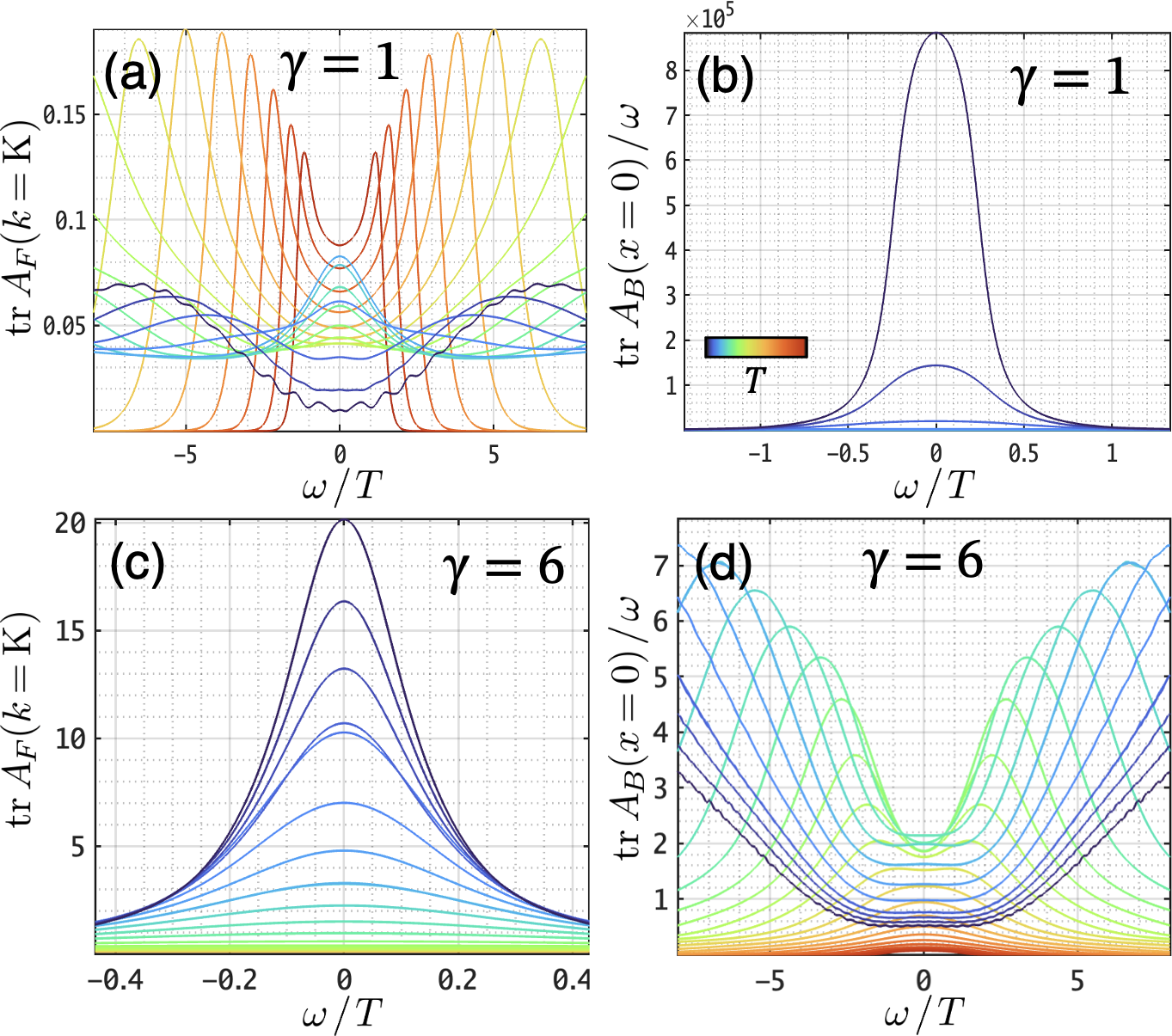
Figure 8: Temperature scaling behavior of the spectral functions of (a)(c) $\mathrm{tr}A_{F}(k\!\!=\!\!\mathrm{K},\omega)$ and (b)(d) $\mathrm{tr}A_{B}(x\!\!=\!\!0,\omega)/\omega$ for the gapless phases. Note that $T$-scaling exponent changes sign across different $\gamma$’s. The ripples in (a) is due to finite size effects. For both cases $J_{K}/t_{c}=6$, and $t_{f}/t_{c}=-0.2$.

At low temperatures, our numerical solutions confirm the form of our conformal ansatzes in Eqs. (Dynamic Mass Generation and Topological Order in Overscreened Kondo Lattices,10). Near the fix point, the form of the 2D Green’s function is governed by the scaling hypothesis $G(\mathbf{r},\tau;T)\sim T^{2\Delta}h(T\mathbf{r},T\tau)$, which in the presence of Lorentz symmetry becomes $G(\vec{r};T)\sim T^{2\Delta}\tilde{h}(T\vec{r})$. It follows that the scaling of spectral functions as shown in Fig. 8 reveals $\Delta_{b,f}$. Although conformal ansatzes would imply that $h\sim\tilde{h}$ is a monomial, in a UV complete theory, the behavior at $\|\vec{q}\,\|=0$ is constrained by the sum rules, e.g., the spectral sum of $(A_{F})_{\kappa\kappa}$ are all 1. This limits any divergence in a scaling ansatz. Indeed, by inspecting Eq. 17 one see that if $A_{F}$ is not quickly diverging, $A_{B}|_{\omega\sim 0}\sim\omega$. For this reason, the bosonic holons $A_{B}(\omega)_{\kappa\kappa}$, odd due to p-h symmetry in our studies, is always an extremum when divided by $\omega$ regardless of $\Delta_{b}$. Thus, we use $T$-scaling behaviors at $\|\vec{q}\,\|\sim 0$ to extract the scaling exponents plotted in Fig. 2(d). That $T$-scaling can change with $\gamma$ from diverging to vanishing gives us a clear anchor for the exponents.

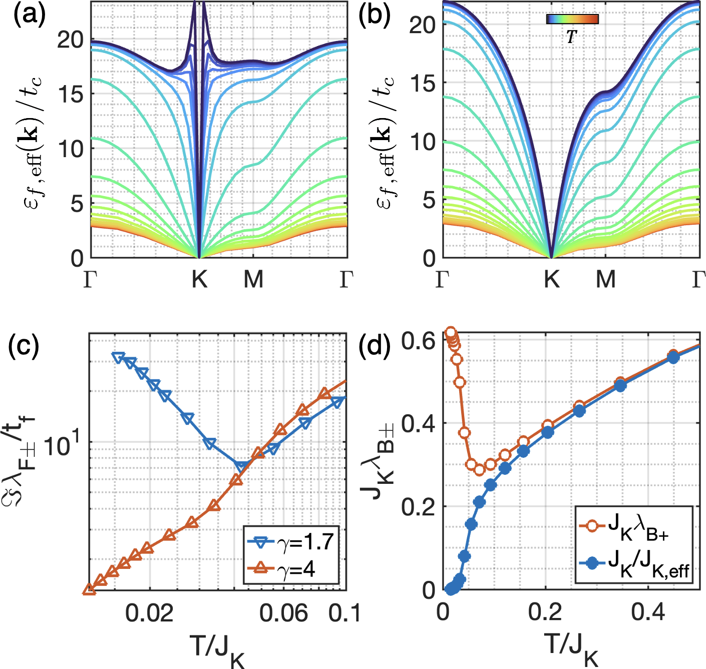
Figure 9: (a–b) Effective energies $\varepsilon_{f}\equiv\Re[-G_{F}^{-1}(k,0+i\eta)]$ of spinons at a $\gamma$ of (a) 1.7 and (b) 4, evolving as temperature cools down. (c) The imaginary part of the eigenvalues $\Im\lambda_{F{\pm}}$ of $-G_{F}^{-1}$ vs. $T$. It is diverging for $\gamma=1.7$ where $\Delta_{f}>3/2$, and vanishing for $\gamma=4$ where $\Delta_{f}<3/2$. (d) The eigenvalues $\lambda_{B{\pm}}$ at $\gamma=1.7$, which are both greater than zero. The lesser one gives $J_{K,\mathrm{eff}}^{-1}$ while the greater one remains finite at $T=0$. For all data $J_{K}/t_{c}=6$, and $t_{f}/t_{c}=-0.2$.

Another import scaling behavior of the Green’s functions lies in their effective energies. The low temperature fixed point in the overscreened Kondo system is marked by the cancellation of bare energies, $\varepsilon_{f}$ and $-1/J_{K}$ by parts of the self energies $\Sigma_{F}$ and $\Sigma_{B}$ respectively, at the critical momenta at $\omega=0$ [17, 49]. The remaining self energies, $\delta\Sigma$’s, constitute the conformally invariant Green’s functions, $-G^{-1}=\delta\Sigma$. The honeycomb lattice has two orbitals per cell. This makes room for nontrivial cancellation of the bare energies as well as the remaining effective energies, $\varepsilon_{f}$ for spinons and $1/J_{K,\mathrm{eff}}$ for holons. They are given by real parts of the eigenvalues $\lambda_{\pm}$ of $-G^{-1}$.

In the case of spinons, $\lambda_{F\pm}$ have opposite real parts and identical imaginary parts due to p-h symmetry, and $\varepsilon_{f}=\Re\lambda_{\pm}$. The magnitudes $\left|\lambda_{\pm}\right|$ can be diverging or vanishing governed by the sign of $3-2\Delta_{f}$, cf. Fig. 2(d). However, $\varepsilon_{f}(\mathbf{k})$ at K and $\mathrm{K}^{\prime}$ is always zero. When $\Delta_{f}>3/2$, this leads to an interesting $\mathbf{k}$-dependence of $\varepsilon_{f}$, as shown in Figs. 9(a)(b). As $\mathbf{k}$ approaches $\mathrm{K}$ or $\mathrm{K}^{\prime}$, $\varepsilon_{f}$ first tend to diverge but plunges to zero at the critical momenta. Meanwhile, the imaginary parts of $\lambda_{\pm}$ shoot up so that its magnitude will obey the conformal ansatz, as shown in Fig. 9(c). This also affects whether the spectral function is growing or vanishing as $\omega\to 0$ at the critical momenta. Finally, we note that similar to our previous 1+1D study [17], Figures 9(a)(b) shows that spontaneous spinon dispersion and dispersion amplification at lower $T$ also occurs in 2+1D.

In the case of holons, $\lambda_{B\pm}>0$ in our studies due to Bose statistics, which requires that $\mathrm{sign}[A_{B}(\omega)]_{\kappa\kappa}=\mathrm{sign}(\omega)$. However, p-h symmetry requires the dispersion of bosons to have both positive and negative branches. In fact, $\lambda_{B\pm}$ for bosons only takes the absolute value of the dispersion “energies”, as demonstrated by a simple p-h symmetric two-level boson, with the levels $\pm E$:

$$G(\omega+i\eta)=\frac{1}{2}\frac{1}{\omega+i\eta-E}+\frac{1}{2}\frac{1}{\omega-i\eta+E}.$$ (42)

Intriguingly, numerical solutions show that only the lesser eigenvalue $\lambda_{B-}$ vanishes at $T=0$, as shown in Fig. 9(d). Its eigenvector is the molecular bonding state $(\begin{matrix}1&1\end{matrix})^{\scriptscriptstyle T}/\sqrt{2}$ in sublattice basis. Therefore, only sublattice-symmetric Kondo screening takes effect at the fixed point while the other sector is gapped.

A.6 F. Free holon population and holon gap

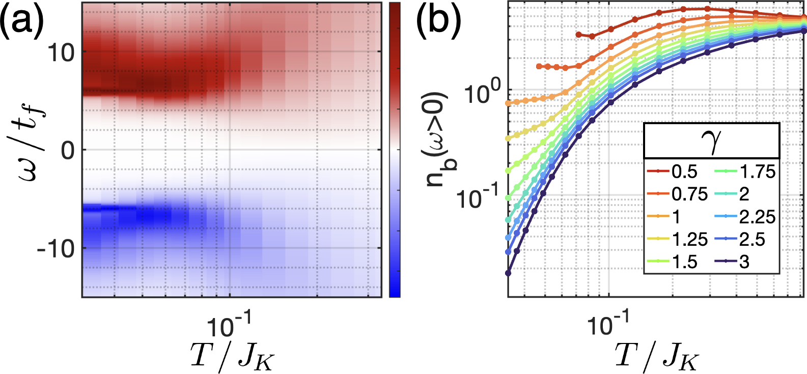
Figure 10: (a) Temperature evolution of the local spectral function of holons in Phase II, corresponding to Fig. 3 in the main text, from which the same parameters are used: $\gamma=5$, $J_{K}/t_{c}=6$, $t_{c}^{\prime}/t_{c}=0.5i$, and $t_{f}/t_{c}=-0.2$. (b) Population of free holons across different $\gamma$’s, corresponding to Fig. 4(c) in the main text, from which the same parameters are used: $J_{K}/t_{c}=6$, $t_{c}^{\prime}/t_{c}=0.5i$, and $t_{f}/t_{c}=-0.4$.

Here we show the population of free holons vs. temperature to supplement the discussion in Figs. 3–4. In panel (a) of Fig. 10, we show that the local holon spectral function in Phase II remains gapped at low $T$, corresponding to Fig. 3 in the main text. Panel (b) of Fig. 10 shows the population of free holons across different $\gamma$’s, corresponding to Fig. 4(c) in the main text. It shows again that at low $T$, $n_{b}(\omega>0)$ is constant in Phase Ia, vanishes by $T^{\xi}$ in Phase Ib, and depletes by $\exp(-m_{b}/T)$ due to the holon gap $m_{b}$ in Phase II.

A.7 G. Mean-field hybridization model for Phase I

Figure 11: The spectral function $\mathrm{tr}A_{F}(k,\omega)$ of spinons in Phase Ia at $\gamma=0.75$, overlaid with a mean-field hybridization model between two $c$-bands and two $f$-bands. Circular data points shows the energy bands of the hybridization model, colored according to $c$ vs. $f$-electron contents. The bare spinon hoppings $\left|t_{f}/t_{c}\right|$ are (a) 0.2, (b) 0.4, (c) 0.6, (d) 1. All hybridizations are set to $V=1.6$, constant in momentum. The dotted lines show the bare energy dispersion of $c$-electrons and $f$-electrons (spinons). Spectral functions of large-$N$ solutions are heavily capped. For all cases, $J_{K}/t_{c}=6$.

In Phase I, spinons are gapped due to inherited Haldane mass from conduction electrons whilst holons develops a coherent gapless mode at $k=\Gamma$. This resembles a uniform hybridization between $c$ and $f$-electrons, of the form $Vc^{\dagger}_{j}f^{\vphantom{\dagger}}_{j}+\mathrm{h.c.}$. As discussed in the main text, this is also the only relevant term that would gap out $f$-electrons starting from zero Haldane mass. Figure 11 shows the energy bands of such a mean-field hybridization model, compare with the dynamical large-$N$ results. One can see the similarity between the resulting spectral functions. Also present are incoherent traces of the (amplified) dispersions of $c$ and $f$-electrons before hybridization near M points in the gap. This feature is absent from Phase II, demonstrating the difference in the mechanism of mass generation between the two phases.

A.8 H. Phase diagram at constant $\gamma$ and varying $t_{f}$

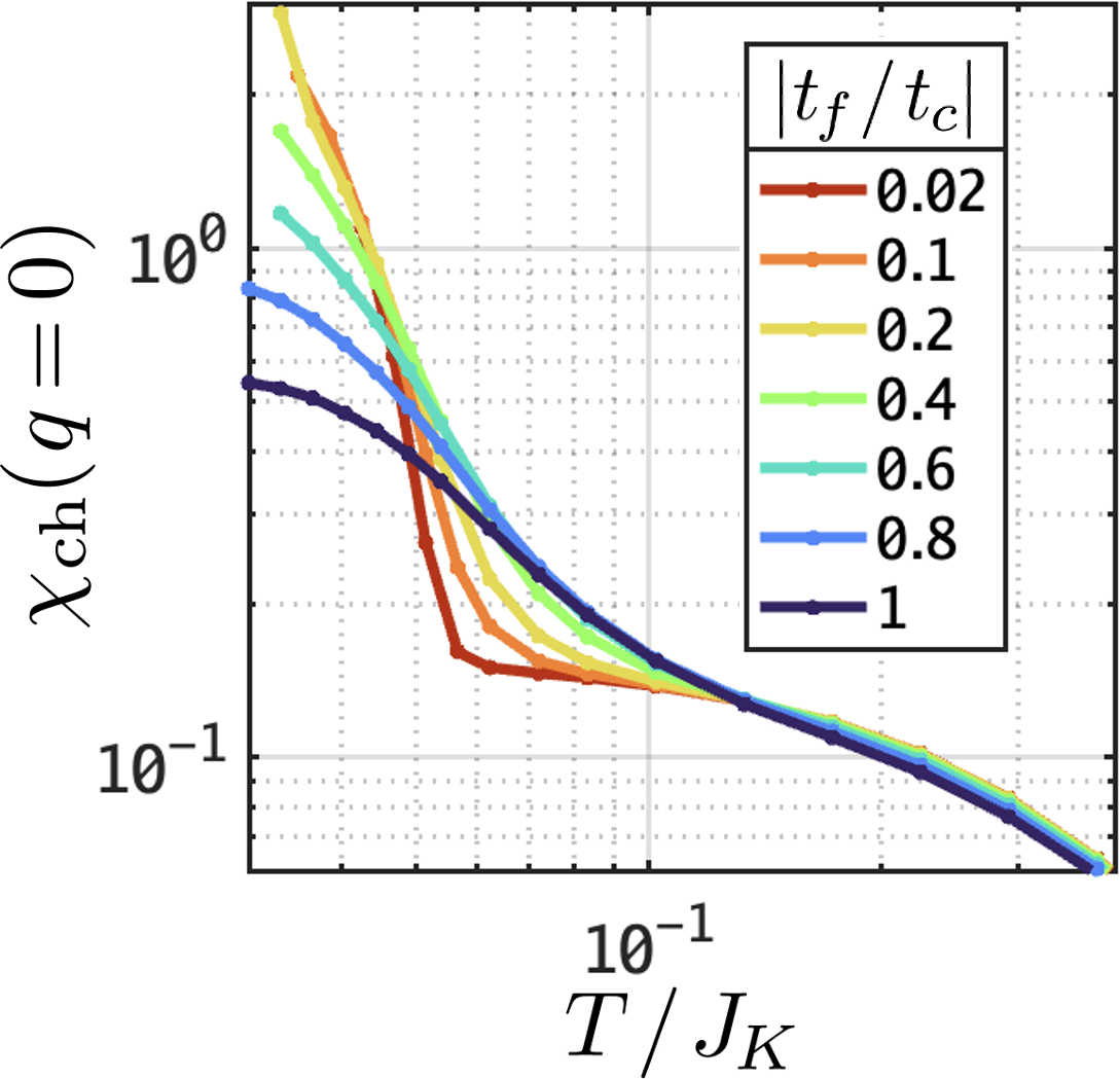
Figure 12: Channel susceptibility across different $t_{f}$’s at a constant $\gamma=1.25$, and with $J_{K}/t_{c}=6$.

The uniform mean-field value for the bond variables $t_{f}$ sets the strength of antiferromagnetic Heisenberg coupling $J_{H}$ in the Abrikosov fermion representation of spins. Our numerics are run at constant $t_{f}$’s, which at low $T$ is equivalent to a constant $J_{H}$. For the gapless phase studies, i.e., with only NN hopping, tuning $t_{f}$ does not change our conformal ansatz nor the scaling exponents. Its only effect is to move the system away from the local Kondo impurity fixed point at high temperatures [17, 49]. A large $t_{f}$ will keep the spinons dispersive at all $T$ and eliminate any trace of this local fixed point where all Green’s functions become essentially local.

In the gapped phase, on the other hand, tuning $t_{f}$ has similar effect to increasing $\gamma$ in the phase diagram, as seen in Fig. 12. Although smaller $t_{f}$ delays the departure from the local Kondo fixed point at higher $T$ when temperature cools down, at $T\to 0$ we see that an increasing $t_{f}$ changes the uniform channel susceptibility from divergent to regular. The magnetic susceptibility is always regular at low $T$ due to the spinon gap.

References

- Andrei and Destri [1984] N. Andrei and C. Destri, Solution of the multichannel Kondo problem, Phys. Rev. Lett. 52, 364 (1984).
- Affleck et al. [1992] I. Affleck, A. W. W. Ludwig, H.-B. Pang, and D. L. Cox, Relevance of anisotropy in the multichannel Kondo effect: Comparison of conformal field theory and numerical renormalization-group results, Phys. Rev. B 45, 7918 (1992).
- Emery and Kivelson [1992] V. J. Emery and S. Kivelson, Mapping of the two-channel Kondo problem to a resonant-level model, Phys. Rev. B 46, 10812 (1992).
- Affleck and Ludwig [1993] I. Affleck and A. W. W. Ludwig, Exact conformal-field-theory results on the multichannel Kondo effect: Single-fermion Green’s function, self-energy, and resistivity, Phys. Rev. B 48, 7297 (1993).
- Lopes et al. [2020] P. L. S. Lopes, I. Affleck, and E. Sela, Anyons in multichannel Kondo systems, Phys. Rev. B 101, 085141 (2020).
- Komijani [2020] Y. Komijani, Isolating Kondo anyons for topological quantum computation, Phys. Rev. B 101, 235131 (2020).
- Kornjaca et al. [2021] M. Kornjaca, V. L. Quito, and F. Rebecca, Mobile Majorana zero-modes in two-channel Kondo insulators, arXiv:2104.11173 (2021).
- Cox and Jarrell [1996] D. L. Cox and M. Jarrell, The two-channel Kondo route to non-Fermi-liquid metals, J. Phys. Condens. Matter 8, 9825 (1996).
- Hewson [1993] A. C. Hewson, The Kondo Problem to Heavy Fermions, Cambridge Studies in Magnetism (Cambridge University Press, 1993).
- Si et al. [2014] Q. Si, J. H. Pixley, E. Nica, S. J. Yamamoto, P. Goswami, R. Yu, and S. Kirchner, Kondo destruction and quantum criticality in Kondo lattice systems, J. Phys. Soc. Jpn. 83, 061005 (2014).
- Coleman [2015] P. Coleman, Introduction to Many-Body Physics (Cambridge University Press, 2015).
- Onimaru and Kusunose [2019] T. Onimaru and H. Kusunose, Exotic quadrupolar phenomena in non-Kramers doublet systems — the cases of PrZn20 ( = Ir, Rh) and PrAl20 ( = V, Ti) —, J. Phys. Soc. Jpn. 85, 082002 (2019).
- Patri and Kim [2020] A. S. Patri and Y. B. Kim, Critical theory of non-Fermi liquid fixed point in multipolar Kondo problem, Phys. Rev. X 10, 041021 (2020).
- Wen [1990] X. G. Wen, Topological orders in rigid states, Int. J. Mod. Phys. B 04 (1990).
- Hoshino et al. [2011] S. Hoshino, J. Otsuki, and Y. Kuramoto, Diagonal composite order in a two-channel Kondo lattice, Phys. Rev. Lett. 107, 247202 (2011).
- Schauerte et al. [2005] T. Schauerte, D. L. Cox, R. M. Noack, P. G. J. van Dongen, and C. D. Batista, Phase diagram of the two-channel Kondo lattice model in one dimension, Phys. Rev. Lett. 94, 147201 (2005).
- Ge and Komijani [2022] Y. Ge and Y. Komijani, Emergent Spinon Dispersion and Symmetry Breaking in Two-Channel Kondo Lattices, Phys. Rev. Lett. 129, 077202 (2022).
- Van Dyke et al. [2019] J. S. Van Dyke, G. Zhang, and R. Flint, Field-induced ferrohastatic phase in cubic non-Kramers doublet systems, Phys. Rev. B 100, 205122 (2019).
- Zhang et al. [2018] G. Zhang, J. S. Van Dyke, and R. Flint, Cubic hastatic order in the two-channel Kondo-Heisenberg model, Phys. Rev. B 98, 235143 (2018).
- Wugalter et al. [2020] A. Wugalter, Y. Komijani, and P. Coleman, Large- approach to the two-channel Kondo lattice, Phys. Rev. B 101, 075133 (2020).
- Jarrell et al. [1996] M. Jarrell, H. Pang, D. L. Cox, and K. H. Luk, Two-channel Kondo lattice: An incoherent metal, Phys. Rev. Lett. 77, 1612 (1996).
- Jarrell et al. [1997] M. Jarrell, H. B. Pang, and D. L. Cox, Phase diagram of the two-channel Kondo lattice, Phys. Rev. Lett. 78, 1996 (1997).
- Hoshino and Kuramoto [2015] S. Hoshino and Y. Kuramoto, Collective excitations from composite orders in Kondo lattice with non-Kramers doublets, J. Phys. Conf. Ser. 592, 012098 (2015).
- Inui and Motome [2020] K. Inui and Y. Motome, Channel-selective non-Fermi liquid behavior in the two-channel Kondo lattice model under a magnetic field, Phys. Rev. B 102, 155126 (2020).
- Grover and Senthil [2008] T. Grover and T. Senthil, Topological spin Hall states, charged skyrmions, and superconductivity in two dimensions, Phys. Rev. Lett. 100, 156804 (2008).
- Komijani et al. [2018] Y. Komijani, A. Toth, P. Chandra, and P. Coleman, Order fractionalization, arXiv:1811.11115 (2018).
- Millis [1992] A. J. Millis, Nearly antiferromagnetic Fermi liquids: An analytic Eliashberg approach, Phys. Rev. B 45, 13047 (1992).
- Altshuler et al. [1995] B. L. Altshuler, L. B. Ioffe, A. I. Larkin, and A. J. Millis, Spin-density-wave transition in a two-dimensional spin liquid, Phys. Rev. B 52, 4607 (1995).
- Sachdev et al. [1995] S. Sachdev, A. V. Chubukov, and A. Sokol, Crossover and scaling in a nearly antiferromagnetic fermi liquid in two dimensions, Phys. Rev. B 51, 14874 (1995).
- Abanov et al. [2003] A. Abanov, A. V. Chubukov, and J. Schmalian, Quantum-critical theory of the spin-fermion model and its application to cuprates: Normal state analysis, Adv. Phys. 52, 119 (2003).
- Oganesyan et al. [2001] V. Oganesyan, S. A. Kivelson, and E. Fradkin, Quantum theory of a nematic fermi fluid, Phys. Rev. B 64, 195109 (2001).
- Metzner et al. [2003] W. Metzner, D. Rohe, and S. Andergassen, Soft fermi surfaces and breakdown of fermi-liquid behavior, Phys. Rev. Lett. 91, 066402 (2003).
- Chowdhury and Sachdev [2014] D. Chowdhury and S. Sachdev, Density-wave instabilities of fractionalized fermi liquids, Phys. Rev. B 90, 245136 (2014).
- Mross et al. [2010] D. F. Mross, J. McGreevy, H. Liu, and T. Senthil, Controlled expansion for certain non-fermi-liquid metals, Phys. Rev. B 82, 045121 (2010).
- Metlitski et al. [2015] M. A. Metlitski, D. F. Mross, S. Sachdev, and T. Senthil, Cooper pairing in non-fermi liquids, Phys. Rev. B 91, 115111 (2015).
- Mahajan et al. [2013] R. Mahajan, D. M. Ramirez, S. Kachru, and S. Raghu, Quantum critical metals in dimensions, Phys. Rev. B 88, 115116 (2013).
- Fitzpatrick et al. [2013] A. L. Fitzpatrick, S. Kachru, J. Kaplan, and S. Raghu, Non-fermi-liquid fixed point in a wilsonian theory of quantum critical metals, Phys. Rev. B 88, 125116 (2013).
- Fitzpatrick et al. [2014] A. L. Fitzpatrick, S. Kachru, J. Kaplan, and S. Raghu, Non-fermi-liquid behavior of large- quantum critical metals, Phys. Rev. B 89, 165114 (2014).
- Torroba and Wang [2014] G. Torroba and H. Wang, Quantum critical metals in dimensions, Phys. Rev. B 90, 165144 (2014).
- Fitzpatrick et al. [2015] A. L. Fitzpatrick, G. Torroba, and H. Wang, Aspects of renormalization in finite-density field theory, Phys. Rev. B 91, 195135 (2015).
- Metlitski and Sachdev [2010] M. A. Metlitski and S. Sachdev, Quantum phase transitions of metals in two spatial dimensions. ii. spin density wave order, Phys. Rev. B 82, 075128 (2010).
- Lee [2009] S.-S. Lee, Low-energy effective theory of fermi surface coupled with u(1) gauge field in dimensions, Phys. Rev. B 80, 165102 (2009).
- Dalidovich and Lee [2013] D. Dalidovich and S.-S. Lee, Perturbative non-fermi liquids from dimensional regularization, Phys. Rev. B 88, 245106 (2013).
- Lee [2018] S.-S. Lee, Recent developments in non-fermi liquid theory, Annu. Rev. Condens. Matter Phys. 9, 227 (2018).
- Chen et al. [2023] J. Chen, E. M. Stoudenmire, Y. Komijani, and P. Coleman, Matrix product study of spin fractionalization in the 1d kondo insulator, arXiv:2302.09701 (2023).
- Raczkowski et al. [2022] M. Raczkowski, B. Danu, and F. F. Assaad, Breakdown of heavy quasiparticles in a honeycomb kondo lattice: A quantum monte carlo study, Phys. Rev. B 106, l161115 (2022).
- Jerez et al. [1998] A. Jerez, N. Andrei, and G. Zaránd, Solution of the multichannel Coqblin-Schrieffer impurity model and application to multilevel systems, Phys. Rev. B 58, 3814 (1998).
- Parcollet et al. [1998] O. Parcollet, A. Georges, G. Kotliar, and A. Sengupta, Overscreened multichannel Kondo model: Large- solution and conformal field theory, Phys. Rev. B 58, 3794 (1998).
- Parcollet and Georges [1997] O. Parcollet and A. Georges, Transition from overscreening to underscreening in the multichannel Kondo model: Exact solution at large , Phys. Rev. Lett. 79, 4665 (1997).
- Komijani and Coleman [2018] Y. Komijani and P. Coleman, Model for a ferromagnetic quantum critical point in a 1D Kondo lattice, Phys. Rev. Lett. 120, 157206 (2018).
- Rech et al. [2006] J. Rech, P. Coleman, G. Zarand, and O. Parcollet, Schwinger boson approach to the fully screened Kondo model, Phys. Rev. Lett. 96, 016601 (2006).
- Kruthoff et al. [2017] J. Kruthoff, J. de Boer, J. van Wezel, C. L. Kane, and R.-J. Slager, Topological classification of crystalline insulators through band structure combinatorics, Phys. Rev. X 7, 041069 (2017).
- [53] The self-consistency equations are exactly those of Abrikosov fermions, by exchanging Schwinger bosons with bosonic holons and fermionic holons with Abrikosov fermions [54] .
- [54] See supplementary materials .
- Neto et al. [2009] A. H. C. Neto, F. Guinea, N. M. R. Peres, K. S. Novoselov, and A. K. Geim, The electronic properties of graphene, Rev. Mod. Phys. 81, 109 (2009).
- [56] Compared to the low-energy Hamiltonian of the Graphene in [55], we have done a rotation .
- Haldane [1988] F. D. M. Haldane, Model for a quantum Hall effect without Landau levels: Condensed-matter realization of the “parity anomaly”, Phys. Rev. Lett. 61, 2015 (1988).
- Semenoff [2012] G. W. Semenoff, Chiral symmetry breaking in graphene, Physica Scripta T146, 014016 (2012).
- You et al. [2018] Y.-Z. You, Y.-C. He, C. Xu, and A. Vishwanath, Symmetric fermion mass generation as deconfined quantum criticality, Phys. Rev. X 8, 011026 (2018).
- Zeng et al. [2022] M. Zeng, Z. Zhu, J. Wang, and Y.-Z. You, Symmetric mass generation in the 1+1 dimensional chiral fermion 3-4-5-0 model, Phys. Rev. Lett. 128, 185301 (2022).
- Wang and You [2022] J. Wang and Y.-Z. You, Symmetric mass generation, Symmetry 14, 1475 (2022).
- Semenoff et al. [1994] G. W. Semenoff, P. Suranyi, and L. C. R. Wijewardhana, Phase transitions and mass generation in 2+1 dimensions, Phys. Rev. D 50, 1060 (1994).
- Appelquist et al. [1996] T. Appelquist, J. Terning, and L. C. R. Wijewardhana, Zero temperature chiral phase transition in SU() gauge theories, Phys. Rev. Lett. 77, 1214 (1996).
- Wijewardhana [1997] L. C. R. Wijewardhana, Zero temperature phase transitions in gauge theories, Int. J. Mod. Phys. A 12, 1195 (1997).
- Hu et al. [2021] H. Hu, L. Chen, C. Setty, M. Garcia-Diez, S. E. Grefe, A. Prokofiev, S. Kirchner, M. G. Vergniory, S. Paschen, J. Cano, and Q. Si, Topological semimetals without quasiparticles, arXiv:2110.06182 (2021).
- Oshikawa [2000] M. Oshikawa, Topological approach to Luttinger’s theorem and the Fermi surface of a Kondo lattice, Phys. Rev. Lett. 84, 3370 (2000).
- Zamolodchikov [1986] A. B. Zamolodchikov, “Irreversibility” of the flux of the renormalization group in a 2D field theory, JETP Lett. 43, 730 (1986).
- Andrei and Orignac [2000] N. Andrei and E. Orignac, Low-energy dynamics of the one-dimensional multichannel Kondo-Heisenberg lattice, Phys. Rev. B 62, R3596 (2000).
- Azaria and Lecheminant [2000] P. Azaria and P. Lecheminant, Chirally stabilized critical state in marginally coupled spin and doped systems, Nuclear Physics B 575, 439 (2000).
- Azaria et al. [1998] P. Azaria, P. Lecheminant, and A. A. Nersesyan, Chiral universality class in a frustrated three-leg spin ladder, Phys. Rev. B 58, R8881 (1998).
- Andrei et al. [1998] N. Andrei, M. R. Douglas, and A. Jerez, Chiral liquids in one dimension: A non-Fermi-liquid class of fixed points, Phys. Rev. B 58, 7619 (1998).
- Regnault and Bernevig [2011] N. Regnault and B. A. Bernevig, Fractional chern insulator, Phys. Rev. X 1, 021014 (2011).
- Liu and Bergholtz [2023] Z. Liu and E. J. Bergholtz, Recent developments in fractional chern insulators, in Reference Module in Materials Science and Materials Engineering (Elsevier, 2023).
- Sachdev [2018] S. Sachdev, Topological order, emergent gauge fields, and Fermi surface reconstruction, Rep. Prog. Phys. 82, 014001 (2018).
- Tsvelik and Coleman [2022] A. M. Tsvelik and P. Coleman, Order fractionalization in a kitaev-kondo model, Physical Review B 106, 125144 (2022).