U-Park: A User-Centric Smart Parking Recommendation System for Electric Shared Micromobility Services

Abstract

At present, electric shared micromobility services (ESMS) have become an important part of the mobility as a service (MaaS) paradigm for sustainable transportation systems. However, current ESMS suffer from critical design issues such as a lack of integration, transparency and user-centric approaches, resulting in high operational costs and poor service quality. A key operational challenge in ESMS is related to parking, particularly how to ensure a shared vehicle has a parking space when the user is approaching the destination. For instance, our recent study illustrated that up to 12.9% of shared E-bike users in Dublin, Ireland cannot park their E-bikes properly due to a lack of planning and user-centric guidance [1]. To address this challenge, in this paper we propose U-Park, a user-centric smart parking recommendation system for ESMS aiming at making personalised recommendations to ESMS users by considering a given user’s historical mobility data, current trip trajectory and parking space availability. We propose the system architecture, implement it, and evaluate its performance based on a real-world dataset from an Irish-based shared E-bike company, Moby bikes. Our results illustrate that U-Park can effectively predict a user’s destination in a shared E-bike system with around 97.33% accuracy without direct user inputs, and such results can be subsequently used to recommend the best parking station for the user depending on the availability of predicted parking spaces. Finally, a blockchain-empowered module is blended to manage various transactions due to its advantage in safety and transparency in this process, including prepays and parking fines.

I Introduction

With increasing interest in the shared economy and emerging popularity in electric micromobility, electric shared micromobility services (ESMS) have become an important part of the Mobility as a Service (MaaS) framework in modern intelligent transportation systems. Electric shared micromobility options, such as electric bikes (E-bikes) and electric scooters (E-scooters), are becoming particularly popular with the general public [2]. These tools have shown their efficacy in addressing the last-mile problem in cities for commuting and delivering goods mainly over short distances. For instance, a recent study has pointed out that these electrified tools can replace up to 76% short trips made by private fossil fuel cars [3], contributing positively to our living environment. E-bikes, in particular, can also help improve citizens’ health when they are used appropriately [4]. E-scooters, on the other hand, can be propelled fully by using electric power from batteries which do not require any physical inputs from riders, making them an ideal tool for shorter trips. As a result, promoting the uptake of ESMS has become strategically important for many European countries to achieve a sustainable and low-carbon transport system [5, 6, 7, 8]. In Ireland, for instance, the government has established a clear pathway to step up the adoption of electric vehicles for transportation decarbonisation in the next decade with an ambitious target to reduce 51% of transport emissions by 2030.

However, current ESMS suffer from critical design issues, such as lack of service integration and not being user-centric, which potentially significantly impedes mass adoption. In fact, some recent work has demonstrated that ESMS can create various burdens in modern traffic operation and management, including inappropriate parking challenges due to users’ behaviours [1], charging issues due to lack of infrastructures [9], accessibility challenges due to lack of holistic planning and scheduling [10], as well as transaction challenges due to lack of speed and transparency [11, 12]. Typically, these challenges are dealt with either partially or individually without a holistic view of system-level design and optimization, with the result that one problem may be addressed for a given aspect but more problems can be created for others. For instance, a route prediction engine may help predict the potential destinations of a cyclist based on the user’s historical trip records, however, the engine may not be able to tell if the predicted destination (with the highest likelihood) can accommodate the bike for parking at the station upon arrival if the system design is not holistic. On the other hand, the existing payment systems for ESMS are mostly reactive, meaning that no information can be used for cost estimation at the start of a trip, which may lead to the non-ideal situation where the cyclist may have to terminate his/her journey earlier than anticipated due to lack of sufficient credits in the account. Moreover, current payment methods in these systems are also inefficient, meaning that a user may not get his/her money back immediately due to a faulty transaction in using the system. For example, a user may be required to pay a fine for inappropriate parking due to erroneous detection of the user’s parking location as per the Global Positioning System (GPS) signal transmitted to the platform that uses by geofencing for parking localization.

To address the parking challenges, a recent work [13] has shown that 37% of riders believe that a proactive mechanism, e.g., an in-app reminder, to guide riders to available parking spaces would be more beneficial to improve users’ behaviours towards considerate parking, while only 18% of the riders believe that a punishment mechanism at the end of trips would be effective in improving their parking accuracy. Similarly, a large body of work [14, 15, 16, 17, 18, 19, 20, 21, 22, 23, 24, 25, 26, 27, 28] have pointed out that machine learning algorithms and data-driven techniques can be adapted to facilitate recommendation mechanisms for proactive and personalised mobility, including destination prediction and parking availability prediction. However, to the best of the authors’ knowledge, at present, there is no smart parking solution which aims to holistically link different components for ESMS.

Therefore, our objective in this paper is to propose U-Park, a user-centric smart parking recommendation system for ESMS leveraging machine learning techniques. The current paper extends our previous work in a number of ways. In particular, the work in the present paper builds on [1, 29, 30]. In [1], we investigated the parking behaviour of shared E-bike users based on a real-world dataset in a case study in Ireland. The results revealed that up to 12.9% of shared E-bike users did not park their bikes properly at the designated stands, which is clearly a challenge to be addressed. In [29], we devised a spatiotemporal graph neural network with attention mechanisms to accurately predict availability in a bike-sharing system. Our proposed model can achieve a very promising result of 1.00 MAE as the selected performance metric. A key difference between the work in [29] and this work is that our previous work aims to predict the availability of bikes in any given bike station for users at the start of their trips, while this work aims to predict the availability of parking spaces for users to properly terminate their trips. Finally, in [30], we devised a Bayesian classifier for route prediction with Markov chains. The Bayesian classier can take a user’s partial trajectory to update the posterior probabilities of the user’s destination based on the user’s historical trip data. A key limitation of the work was that the model was only validated using a synthetic dataset and the approach was developed based on classical Bayesian inference without comparing with other state-of-the-art approaches, such as deep learning-empowered methods.

Our work builds upon ideas from all three papers to create a user-centric architecture in which a personalised recommendation can be made to ESMS users to help address their parking requirements in a data-driven framework. Specifically, our proposed smart parking recommendation system, U-Park, has several advantages compared to the state-of-the-art system design as it incorporates the following key features:

• U-Park can help address a user’s parking request in ESMS from the start of a journey rather than near the end of a journey in a proactive manner.

• U-Park can operate at all stages for a journey, i.e., pre-journey, in-journey, and post-journey, without necessarily requiring a user’s explicit input, but such information can be accommodated based on a user’s interaction.

• U-Park can dynamically monitor and improve prediction accuracy for parking based on the user’s present trajectory and historical mobility patterns as inputs.

• U-Park can efficiently manage various transaction issues in ESMS through the integration of a blockchain-based component.

The paper is structured as follows. In Section II, we introduced related work in existing ESMS systems and machine learning techniques used in this field. Our research problems are defined and discussed in Section III. Section IV discusses the overall design of our enrollment system. In Section V, we present the details of our prototype implementation. The results and relevant discussions are included in Section VI, and the limitation of our current work is described in Section VII. Finally, we conclude our work in Section VIII and discuss future plans and improvements.

II Literature Review

In this paper, we consider the relevant literature from three perspectives: Current Electric Shared Micro-mobility Services, Machine Learning Methods in Travel Demand Prediction and Machine Learning Methods in Trip Destination Prediction.

II-A Current Electric Shared Micro-mobility Services

II-A1 Inappropriate Parking Behaviours

The improper parking of shared micromobilities will increase the company’s management costs and result in inconveniences for future users and even safety risks for other traffic participants. Thus, a significant number of recent research studies have been conducted on the existence, impacts and solutions relevant to inappropriate parking behaviours [31, 1, 32, 33, 34]. For example, in [31] the authors revealed the existence of inappropriate parking by the analysis of data collected in five cities in the U.S.A, and in [32], the authors reviewed papers related to bicycle parking and indicated the positive impacts on cycling behaviours from the availability of parking spaces.

II-A2 Incentive Policies

The incentive and punishment policies of companies around the world vary. A study [33] investigated some of these policies and suggested that in China, a reward of $1.43$ yuan (i.e., $0.2$ euros) per minute could be used to encourage shared bike users to move to another parking station. Furthermore, the performances of increasing the intensity of incentives and financial penalties were found to differ in terms of encouraging policy compliance, particularly when the shifting distance was longer than a certain distance ($10$ minutes walking in the paper). Nevertheless, the reward amount and shifting distance mentioned above may be subject to the user’s heterogeneous characteristics, such as personal attitudes.

II-A3 Pricing Policies

Pricing policies vary with different devices (e.g., bikes, E-bikes), operators and regions, but most are based on periodic charging methods (e.g., monthly plan) or pay-as-you-go approaches. Since the former is not affected by a single use, this paper only focuses on the pay-as-you-go approach which usually includes an activation fee and billing by the minute. For example, in Dublin, Ireland shared E-bikes provided by MOBY cost a 1 euro start fee and 5 cents per minute, by ESB cost a 1 euro start fee and 15 cents per minute and by Tier cost a 1 euro start fee and 20 cents per minute. Shared E-bikes provided by Lime cost a 1 pound start fee and 19 pence per minute, while shared E-scooters provided by Lime cost a 1 pound start fee and 15 pence per minute, and by Dott cost a 1 pound start fee and 17 pence per minute in London, the UK.

II-A4 Relevant Datasets

The rapid emergence of the sharing economy has been an essential factor in the increased use of shared mobility services, particularly shared bikes. Unfortunately, ESMS systems (e.g., E-bikes and E-scooters) were largely overlooked previously, leading to a lack of detailed datasets on their usage. Although more businesses are investing in these modes of transportation in recent years, the data collected is generally not accessible to the public, resulting in limited research and investigation of them. Some researchers working on ESMS have briefly introduced and presented the datasets used in their studies. In particular, we summarise the common features of the datasets applied in [14, 15, 16, 17] as follows. Usage datasets (e.g., [17]) typically include starting and ending timestamps and GPS locations, the trip duration, and the distance, while trajectory datasets (e.g., [15]) contain timestamps, GPS coordinates (latitudes and longitudes), and vehicle IDs. However, these datasets are not conducive to extracting user-related features, so the predicted results often do not have superior performance when the trained models are applied to different users. Thus, it is currently very difficult to obtain an open data source sufficiently complete in providing detailed GPS time series and parking spaces at each stand.

II-A5 Existing Frameworks

In [22], the authors proposed a two-stage framework for destination prediction. Hand-crafted rules were used to generate candidate destinations in the first stage, then a prediction model is used to predict the output based on the trip and customer attributes from the candidate set. Compared to this framework, our system introduced in Section III used an entirely machine-learning-based model to predict the trip destination, and our system not only focuses on historical trip records but also trip trajectories. That is to say, except for making a basic forecast based on history before the trip starts, our model will make in-journey predictions and recommendations as well. Besides, the framework stopped at destination prediction, but we used the destination as an input to the model in the next stage and concentrated on the parking behaviour of shared E-bike users.

To sum up, it can be seen from the relevant work mentioned above that ESMS systems could be improved by reducing the occurrence of improper parking behaviours [1] which are usually affected by parking space availability [32]. As such, in the following sections, we review and summarise machine learning approaches adopted in the field of ESMS in two aspects – the demand of trips from one location to another and the destination of trips. The latter enables us to predict the ending point of a current journey and accordingly remind the user of parking properly, whereas the former represents the number of departures and arrivals for a particular area or station which determines the parking space availability at that location.

II-B Machine Learning Methods in Travel Demand Prediction

Various machine learning algorithms and models have been applied in hourly demand forecasting of shared micromobilities in different cities worldwide. In this section, previous approaches and techniques used in hourly demand prediction are introduced and summarised in Table I.

TABLE I: Summary of Past Research in Hourly Demand Prediction in Micro-Mobilities.

Object	Case study	Year of publication	Number of valid records	Main model(s) used	Reference
E-bikes	Zurich, Switzerland	2019	72,648	SR, LR	[14]
E-bikes	Ningbo, China	2022	1,774,329	GTWR, OLSR, GWR	[15]
E-scooters	Bangkok, Thailand	2020	28,156	SARIMA, GRACH	[16]
E-scooters	Calgary, Canada	2021	459,478	MFCN, LR, Conv-LSTM	[17]
Bikes	Wenling, China	2021	422,763	STGCN, RNN, LSTM, GRU	[18]
Bikes	Wenling, China	2021	422,763	LSGC-LSTM, RNN, LSTM, GRU, etc.	[19]
Bikes	Seoul, South Korea,	2022	1,685,715	Conv-LSTM, CNN, RNN, LSTM, GCN, etc.	[20]
Bikes	Jersey, U.S.A.	2022	333,802	GRU, ARIMA, LSTM	[21]

• Models marked in bold performed best in the authors’ experiments.

Classic machine learning methods such as Spatial Regression (SR) and Linear Regression (LR) have been applied to predict the hourly demand for shared E-bikes in [14, 15, 16]. For instance, in [15], the authors focused on the prediction of travel demand based on the E-bike data collected in Ningbo, China, and the performance of the proposed method, Geographically and Temporally Weighted Regression (GTWR), is significantly better compared to the baseline models, an Ordinary Least-Squares Regression (OLSR) model and a Geographically Weighted Regression (GWR) model in terms of relative error (i.e., $-1.07\%$ with a comparison to $7.85\%$ for OLSR and $-1.43\%$ for GWR).

Recently, deep learning methods such as Long Short-Term Memory (LSTM) in Recurrent Neural Networks (RNN), Convolutional Neural Networks (CNN) and Graph-CNN (GCN) have also attracted widespread attention in research focusing on micromobilities [20, 17, 19, 18, 29]. RNN and LSTM models and their variants are widely applied to capture temporal features in previous papers, for example, the authors used Convolutional LSTM (Conv-LSTM) in [20] in the next-hour bicycle demand based on the rental and return histories of bike-sharing and meteorological data. GCN-based methods are also gradually applied in this prediction task due to their ability to capture the locality of non-Euclidean data effectively [19]. In [18], the authors predicted the picking up and returning demand for bikes based on the proposed Spatio-Temporal Graph Convolutional Network (STGCN) model which achieved better results in prediction accuracy and computation efficiency compared with three baseline models, i.e., RNN, LSTM and Gated Recurrent Unit (GRU). As a popular technique mimicking physiological cognitive attention in deep learning, attention has been used to enhance the prediction performance of GCN models. In our previous work, an Attention-based Spatio-Temporal Graph Convolutional Network (ASTGCN) was proposed and applied in [29] to predict the number of available bikes in each bike parking station. Compared with other existing methods e.g., STGCN and XGBoost (eXtreme Gradient Boosting), this approach has achieved a preferable performance in the prediction task regarding the experiments on realistic datasets. Our current work also follows these ideas. Specifically, we adopt the seminal idea proposed in [29] for the design of the parking space availability prediction module in the proposed ESMS architecture.

Finally, a large body of work has also revealed that the accuracy of the forecasting results could also be affected by spatial attributes (e.g., origin, destination), temporal attributes (e.g., the hour of the day, the day of the week) and weather (e.g., temperature, wind speed, probability of precipitation) [14, 15, 20, 18, 19], so these journey attributes have also been included in the machine learning-based method we adopted in the work reported here. Please note, in this section, we only introduced several machine learning algorithms or models in detail and refer interested readers to Table I for more details of the works [14, 15, 16, 17, 18, 19, 20, 21].

II-C Machine Learning Methods in Trip Destination Prediction

Methods and models used in trip destination prediction adopted in relevant papers have been summarised in Table II and selected works are introduced in detail below. Generally speaking, the prediction of travel destinations could be divided into two types according to the data used in the models, i.e., trip report data and GPS data. Trip report datasets provide temporal and spatial information on the origin and destination of each travel. Auto-Regressive Integrated Moving Average (ARIMA), Conv-LSTM, CNN, GCN and other methods have been adopted and implemented to predict the destination based on trip report data in [24, 23, 22]. For example, in [23], a Destination Prediction Network based on Spatio-Temporal data (DPNst) was designed and implemented based on three models – LSTM, CNN and Fully Connected Neural Network – to extract user behaviour, spatial features and external features (e.g., weather, temperature) respectively. This model was evaluated on the Mobike dataset collected in Beijing, China, and its superiority was then demonstrated with the comparison to Naive Bayesian (NB) [30], basic LSTM and CNN models.

TABLE II: Summary of Past Research in Destination Prediction in Micro-Mobilities.

Object	Case study	Year of publication	Number of valid data	Main model(s) used	Reference
Bike trip report	China	2019	5,445,449	XGBoost, Neural Network	[22]
Bike trip report	Beijing, China	2019	3 millions	DPNst, LSTM, CNN	[23]
Bike trip report	New York, U.S.A.	2021	9 millions	HC-LSTM, ARIMA, Conv-LSTM, GCN, etc.	[24]
Bike trip report	Chattanooga, U.S.A.	2021	400,540	AB-CNN, CF, MART, etc.	[25]
Multi-GPS data	Changchun, China	2019	1,341,510 points	HMM & MNL, Markov chain	[26]
Multi-GPS data	Beijing, China,	2020	13 thousands trips	Conv-LSTM, MLP, GRU, LSTM, CNN, etc.	[27]
Multi-GPS data	China	2022	18,670 trips	MDLN, MLP, RNN, LSTM, etc.	[28]

• Models marked in bold performed best in the authors’ experiments, and numbers marked in italic are the approximations of the dataset sizes.

In parallel, research related to destination prediction based on GPS data has also been explored by many researchers on other objects [27, 26, 28]. For instance, in [28], the authors proposed a Multi-module Deep Learning Network (MDLN) to solve the problem in the task of destination prediction. As the journey trajectory is a temporally-ordered GPS location collection, RNN [35] and LSTM [27] are also widely used in trajectory-based destination prediction due to their outstanding ability to work with temporal and sequential data. Specifically, the authors of [35] applied RNN to model the taxi behaviour based on the trip history and the geographical information, and the authors of [27] compared the Conv-LSTM model with prevalent techniques such as Multi-Layer Perceptron (MLP), GRU, LSTM, and CNN and indicated the advantages of the methods they proposed. It is worth mentioning that some recent research has shown that in a GPS trajectory series, the first $k$ points and the last $k$ points close to the origin and destination of a trip will make a significant contribution to destination prediction tasks [36, 28, 37], so the same method is adopted in our work. Again, we only introduced several machine learning algorithms or models in this section in detail and we suggest interested readers should refer to Table II for more details of the works [22, 23, 24, 25, 26, 27, 28].

To sum up, in addition to spatial and temporal information of the origin and destination of a trip, external attributes, e.g., weather and Point of Interest (i.e., POI), are also widely taken into consideration in machine learning algorithms or models used in both hourly demand and destination prediction work [15, 21, 23, 24]. The RNN model plays an active and essential role in both tasks mentioned above [17, 18, 19, 20, 21, 23, 24, 27, 28] given its usefulness in time-series prediction problems. . Thus, considering the model cost and prediction accuracy, we decided to implement the destination prediction at the beginning of the trip based on trip reports with a simple neural network and during the trip based on GPS data with an RNN model in our work.

III System Model

In this section, we present an overall statement of our research problem and introduce each question in detail. We use a shared E-bike system as an example of ESMS systems for clearer expression; however, U-Park is applicable to other ESMS systems as well. We divide the user journey into three stages: pre-journey (from the moment a user decides to start a trip and scans the QR code attached to the E-bike until it is unlocked), in-journey (from unlocking the bike until the user is close enough to their destination and about to end this trip) and post-journey (from when the user is nearly finished with this trip until he or she has received final recommendations from U-Park, locked up the bike and finished payment). Specifically, if the user’s current position is close enough (e.g., within $dis$ metres) to the predicted destination, we consider the trip to be ending.

III-A Overall Research Problem

Notations: In general, the main purpose of U-Park is to solve improper parking behaviours in ESMS by providing recommendations for parking stations when a journey is about to be completed. Given this context, we can formulate the parking station recommendation problem. For an ESMS system, there are $S$ pre-defined parking stations specified by the operator; thus, the set of parking stations $\mathbb{S}$ are introduced as follows:

$$\mathbb{S}=\{s_{1},s_{2},\dots,s_{S}\}$$ (1)

and for an existing user, there are $N$ trips in total in this user’s historical record $\mathbb{H}$ and GPS report $\mathbb{G}$ retrospectively stored in this ESMS. Based on $\mathbb{H}$ and $\mathbb{G}$, we aim to design a system to make recommendations on the appropriate parking station around the destination of a currently ongoing trip as soon into the trip as possible. Here, we use $\mathbb{T}_{i}$ to represent the $i^{th}$ trip of this user and for each trip $\mathbb{T}_{i}$, we define the GPS report $\mathbb{T}_{i}^{G}$ and the historical record $\mathbb{T}_{i}^{H}$ of it as follows.

Firstly, let us define a GPS report of a single trip $\mathbb{T}_{i}^{G}$ by

$$\mathbb{T}_{i}^{G}=[(t_{1}^{i},p_{1}^{i});(t_{2}^{i},p_{2}^{i});\dots;(t_{L_{i}}^{i},p_{L_{i}}^{i})]$$ (2)

where the sequences $(t_{1}^{i},\dots,t_{L_{i}}^{i})$ and $(p_{1}^{i},\dots,p_{L_{i}}^{i})$ represent the lists of timestamps and GPS positions with the same length, i.e., $L_{i}$. Thus, the size of $\mathbb{T}_{i}^{G}$ is $L_{i}\times 2$. The first position $p_{1}^{i}$ and the last position $p_{L_{i}}^{i}$ indicate the origin and destination of the trip $\mathbb{T}_{i}^{G}$ while the first timestamp $t_{1}^{i}$ and last timestamp $t_{L_{i}}^{i}$ represent its departure time and arrival time. Given the context above, the user’s historical record of a single trip $\mathbb{T}_{i}^{H}$ is defined as:

$$\mathbb{T}_{i}^{H}=[(t_{1}^{i},p_{1}^{i},t_{L_{i}}^{i},p_{L_{i}}^{i})]$$ (3)

which means the history of one specific trip $\mathbb{T}_{i}^{H}$ contains the spatial and temporal features of its origin and destination and the size of $\mathbb{T}_{i}^{H}$ is $1\times 4$. Based on the context given above, the user’s historical record of $N$ trips is:

$$\mathbb{H}=\{\mathbb{T}_{1}^{H},\mathbb{T}_{2}^{H},\dots,\mathbb{T}_{N}^{H}\}$$ (4)

and similarly, the user’s GPS report of $N$ trips is:

$$\mathbb{G}=\{\mathbb{T}_{1}^{G},\mathbb{T}_{2}^{G},\dots,\mathbb{T}_{N}^{G}\}$$ (5)

Finally, based on the list of all trip destinations in this user’s GPS report, i.e., $(p_{L_{1}}^{1},p_{L_{2}}^{2},\dots,p_{L_{N}}^{N})$, we define the set of destinations of this user as follows:

$$\mathbb{D}=\{d_{1},d_{2},\dots,d_{D}\}$$ (6)

where any $d_{j}\in\mathbb{D}$ represents a unique destination, and $D$ is the length of $\mathbb{D}$, so for any existing trip $\mathbb{T}_{i}$ in $\mathbb{G}$, we have the destination $p_{L_{i}}^{i}\in\mathbb{D}$.

Problem: For an ongoing trip $\mathbb{T}_{k}=[(t_{1}^{k},p_{1}^{k});\dots)]$, the overall objective of our U-Park system is to decide an appropriate parking station $\hat{s_{k}}\in\mathbb{S}$ and make recommendations accordingly so that the user is more likely to obtain an available parking space around the destination $\hat{d_{k}}\in\mathbb{D}$ predicted by machine-learning models in U-Park.

Remark: The $\mathbb{S}$ and $\mathbb{D}$ defined in this section refer to different sets. The former is the pre-defined station set and the latter is the set of destinations of this user’s previous trips. The destinations may or may not be included in $\mathbb{S}$. To solve our overall research question, we divide it into three machine-learning tasks in the three stages introduced above. Here, we define the problems to be solved as follows and present them in detail in the following sections: (i) history-based destination prediction in the pre-journey stage; (ii) trajectory-based destination prediction in the in-journey stage; and (iii) parking space availability prediction in the post-journey stage.

III-B History-Based Destination Prediction

Notations: As introduced above, this history-based prediction model is applied at the pre-journey stage aiming to predict the destination of this trip. In addition to the departure and arrival timestamp and position introduced in (3), for a specific trip $\mathbb{T}_{k}$, a set of extra features $f_{k}^{H}$, such as temporal features (e.g., day of the week) and weather conditions (e.g., temperature), is also included for model training. Denoting $N_{f}^{H}$ as the number of $f_{k}^{H}$, the length of the extended historical record of $\mathbb{T}_{k}$ would be $M_{H}=N_{f}^{H}+4$. In other words, the size of the extended historical record of $N$ trips in total would be $N\times M_{H}$.

Problem: For a trip about to begin $\mathbb{T}_{k}=[(t_{1}^{k},p_{1}^{k},f_{k}^{H})]$, the research question at this stage is to solve the classification task of deciding what category in $\mathbb{D}$ the trip $\mathbb{T}_{k}$ belongs to, or in other words, to decide a $d_{H}^{k}\in\mathbb{D}$ for $\mathbb{T}_{k}$.

Remark: This problem is solved every time a user is authorised to unlock a vehicle in this ESMS. Since the model is only determined by the user’s historical record and external features, the prediction result for the current trip $\mathbb{T}_{k}$ will never change.

III-C Trajectory-Based Destination Prediction

Notations: As discussed above, this trajectory-based prediction model is applied at the in-journey stage aiming at improving the prediction result made at the pre-journey stage. In addition to the timestamp and GPS position sequences in (2), for a specific trip $\mathbb{T}_{k}$ with a length of $L_{k}$, a set of extra features $f_{k}^{G}$, such as temporal features (e.g., day of the week) and weather conditions (e.g., temperature) obtained for each timestamp, is also included for model training. Denoting $N_{f}^{G}$ as the number of $f_{k}^{G}$, the size of the extended GPS report of $\mathbb{T}_{k}$ could be presented by $L_{k}\times M_{G}$, where $M_{G}=N_{f}^{G}+2$ indicates the number of features for every timestamp.

Problem: At this stage, the research question for this ongoing trip $\mathbb{T}_{k}=[(t_{1}^{k},p_{1}^{k},f_{k}^{G});(t_{2}^{k},p_{2}^{k},f_{k}^{G});\dots]$ is to solve the classification task of deciding what category in $\mathbb{D}$ the trip $\mathbb{T}_{k}$ belongs to, or in other words, to decide a $d_{G}^{k}\in\mathbb{D}$ for $\mathbb{T}_{k}$.

Remark: Concerning General Data Protection Regulation (GDPR), GPS data will be converted and then entered into our system rather than entered directly. The processing of GPS data will be introduced in Section V. This problem is solved whenever a new GPS position is observed during the current trip. Since this model is determined by external features and the user’s trajectory in real-time, it is possible to update the prediction result of the destination when we include a new GPS point.

III-D Parking Space Availability Prediction

Notations: Last but not least, we formulate the parking space availability prediction problem as follows. Let $A_{t}^{k}$ be the number of available parking docks or spaces at station $s_{k}\in\mathbb{S}$ at time $t$. $\textbf{A}_{t}$ denotes the vector consisting of the numbers of the available parking docks or spaces at all $S$ stations in total at time $t$, so the length of $\textbf{A}_{t}$ is $S$. Additionally, we let $f_{t}^{k}$ denote the value of external features at station $s_{k}$ at time $t$ for model training such as temporal features (e.g., day of the week) and weather conditions (e.g., temperature), and we let $M_{F}$ represent the length of $f_{t}^{k}$. Similarly, we let $\textbf{f}_{t}$ be the feature set values of all parking stations at time $t$. Consequently, the size of $\textbf{f}_{t}$ is $S\times M_{F}$.

Problem: Mathematically, the learning objective of this prediction model, which is applied in the post-journey stage, is to find a function $\textbf{H}(.)$ which addresses the following problem:

$$\textbf{A}_{t+1:t+n}=\textbf{H}(\textbf{A}_{t-m+1:t};\textbf{f}_{t-m+1:t})$$ (7)

where $m$ and $n$ represent the input and output length of this model respectively. Besides, $t+1:t+y$ denotes the output as a sequence of vectors from time $t+1$ to $t+y$.

Remark: The prediction for this problem keeps being made till the destination of the current trip is confirmed by the user, or according to the distance to locations with the most occurrences in predictions. This model is determined by the arrival time and external features, and the arrival time could be obtained by various map APIs.

Here, we introduce the effect of arrival time on the prediction result with an example. A user starts the trip at 10 am and the arrival time estimated by a map API is 11 am. The predicted results for parking space availability will differ from time to time, e.g., at 10 am and 10:50 am in this sample. In practice, the availability can be updated at every fixed time interval, e.g., every 10 minutes. Thus, this prediction model will generate six values for a given hour and the result of the prediction made at 10 am will be the sixth output, while at 10:50 am the result will be the first output, and the accuracy will differ in these two cases.

IV System Architecture

This section presents the proposed framework structure, U-Park, to address the research questions discussed in Section III. An overview of the system architecture is provided in Fig. 1, with hardware and user interface modules involved in all three journey stages - pre-journey, in-journey, and post-journey - as defined in the previous section. Again, we use a shared E-bike system as an example of ESMS systems for clearer expression.

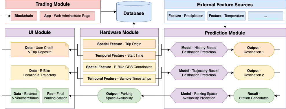
Figure 1: The proposed system architecture for U-Park.

This system, U-Park, consists of three main modules: a hardware module (e.g., E-bikes with multiple sensors attached), a user interface module (e.g., a mobile application), and a prediction module based on machine learning prediction algorithms. Additionally, it also incorporates some external feature sources, a database and a trading module based on a web administration application and blockchain technology to manage financial transactions securely.

IV-A Hardware Module

The hardware module attached to U-Park’s E-bikes will have three main functions: collecting physical data from the bikes, calculating trip deposits, and controlling motor rotation. This module can be built on a single-board computer (SBC, e.g., a Raspberry Pi) with various sensors connected to interact with the cloud database. When an unlocking or locking request is received, the SBC will unlock or lock the E-bike accordingly and calculate the trip deposit, and the motor status would be stored in the database and updated dynamically throughout its duration; additionally, this module will upload the GPS coordinates of E-bikes to our database so that both administrators and users can obtain the current locations of E-bikes.

IV-B User Interface Module

An Android mobile application is developed to provide the users with an interactive interface, accept output from the prediction model and transfer data with the blockchain module. The temporal and spatial information of a trip origin will be transmitted to the pre-trained prediction model, and the results would be sent back as a recommendation. User credits will be transferred and calculated for payments and balances and the user data collected would be uploaded to our database via the trading module. Besides, a map API and QR code scanning function would be adopted to enable users to view their current position and E-bikes around or unlock available E-bikes by scanning with their phones.

When a user opens and logs in on the mobile APP, the user’s position would be visualised based on the GPS coordinates obtained from the user’s smartphone. At the same time, positions and the availability of E-bikes will also be demonstrated by markers in different colours on the map (e.g., in Fig. 6). Additionally, the user is allowed to enter a position as his or her planned destination $d_{U}^{k}$ for a trip $\mathbb{T}_{k}$, once our system obtains the user-planned destination $d_{U}^{k}$, U-Park will skip destination prediction and move to the post-journey stage, as defined in Section III. Thus, considering more complex and universal situations, we focus on the circumstance when the user does not enter the planned destination.

When clicking an available E-bike marker, the user could scan the QR code attached to the E-bike to enter the process of credit validation and deposit payment. The deposit calculation is calculated by (10) and explained in detail in the next section because it is highly related to the prediction results. Generally speaking, the deposit amount is directly determined by the total duration from the trip origin to the predicted destination decided by the history-based model introduced in Section III. If the credit remaining is enough to cover the deposit calculated, the device will be unlocked after the payment and the journey state in our database will be updated. Otherwise, the user would be suggested to top up and try again.

The GPS data of this E-bike will be continuously captured and uploaded until the user ends the trip via their phone. Upon completion, the balance amount $F_{balance}$ is calculated by (8), which is determined by the trip duration, the minimum distance to pre-defined stations and the deposit paid at the start of this trip.

$$F_{balance}=f\cdot(t_{L_{k}}^{k}-t_{1}^{k})+F_{parking}-F_{deposit}$$ (8)

In (8), $f$ represents the charge per second, $t_{L_{k}}^{k}$ is the actual timestamp arriving at the real destination $d_{k}$ and $F_{parking}$ means the pre-defined parking fee defined in Section V. $F_{balance}\geq 0$ means we need to charge the user again at the end of the trip and if $F_{balance}<0$ we should provide a refund.

IV-C Prediction Module

The prediction module is designed to provide suggestions on the parking stations around trip destinations. There are two prediction tasks in total: destination prediction and parking space availability prediction.

Taking into consideration the great impact that destination prediction has on the performance of the next task, we decided to adopt a two-step prediction model. Firstly, when users decide to start a trip from a specific stand, we predict a list of possible destinations (i.e., a set of $d_{H}^{k}$) using our history-based prediction model and then improve the accuracy by leveraging the result of our trajectory-based prediction module (i.e., $d_{G}^{k}$). In other words, the work of destination prediction will be performed in two stages – pre-journey and in-journey – and the trip destination finally estimated by our prediction module $\hat{d_{k}}$ is determined by both $d_{H}^{k}$ and $d_{G}^{k}$.

The workflow of the entire prediction module is illustrated in Fig. 2, where items coloured yellow, orange and green represent history-based and trajectory-based destination predictions as well as the parking space availability prediction respectively. Moreover, the red item summarizes the final result of the destination prediction task while the blue items calculate probability distributions to make a final recommendation regarding which parking station to use. For clarity, we summarise the notations used for destination prediction in Table III.

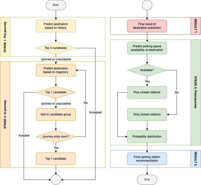
Figure 2: Prediction module workflow.

TABLE III: Notations for destination prediction tasks.

Notation	Explanation
$d_{k}$	the actual destination of trip $\mathbb{T}_{k}$ which will be recorded when the journey ends
$d_{H}^{k}$	the predicted destination of trip $\mathbb{T}_{k}$ which is decided by our history-based model
$d_{G}^{k}$	the predicted destination of trip $\mathbb{T}_{k}$ which is decided by our trajectory-based model
$d_{U}^{k}$	the user-planned destination of trip $\mathbb{T}_{k}$ which is determined by the user when the journey starts
$\hat{d_{k}}$	the overall result of the destination prediction module which is determined by $d_{H}^{k}$ and $d_{G}^{k}$
$\hat{s_{k}}$	the overall result of U-Park, the final parking station recommended to the user when $\hat{d_{k}}$ is decided

IV-C1 Pre-journey

In this stage, the main task of our prediction module is to predict the destination based on the user’s history. Adopting a probabilistic classifier, the classification model introduced in Section III is able to a probability distribution over a set of categories rather than the most likely category, so instead of predicting only one result, we accept multiple outcomes (e.g., three results) with the highest probabilities as the destination candidates and accordingly calculate the deposit $F_{deposit}$ of this trip.

Following the previous notations, when a user decides to unlock an E-bike and start a trip $\mathbb{T}_{k}$ from the origin $p_{1}^{k}$, necessary data (i.e., departure location, starting time, weather conditions and the remaining battery capacity) would be collected by U-Park and used as the input to our prediction model. Specifically, the temporal, spatial and weather-related data will be used in destination prediction, while the remaining battery capacity will be compared with the expected travelling distance or time to examine if the remaining battery is enough to complete this trip. If not, U-Park will help the user find other E-bikes applicable to this trip. Then, the predicted destination candidates $\mathbb{D}_{H}^{k}$, i.e., a set of $d_{H}^{k}$, will then be recommended to the user for confirmation, and depending on the user responses, two cases are considered in this step.

Case 1: If any predicted result $d_{x}$ in $\mathbb{D}_{H}^{k}$ is the same as $d_{U}^{k}$ (i.e., $\exists d_{x}\in\mathbb{D}_{H}^{k}$ $d_{x}=d_{U}^{k}$) and the user confirms it by selecting it from the list given in our mobile app, e.g., in Fig. 3(a), we denote this case by $d_{U}^{k}\in\mathbb{D}_{H}^{k}$ and our prediction module will adopt $d_{U}^{k}$ as the final destination result (i.e., $\hat{d}_{k}\leftarrow d_{U}^{k}$), which will be used to calculate the deposit. The system will then move directly to the post-journey stage without any further destination prediction. Mathematically, the deposit for trip $\mathbb{T}_{k}$ is determined by the timestamp $t_{U}^{k}$ arriving at $d_{H}^{k}$, which is estimated by maps API.

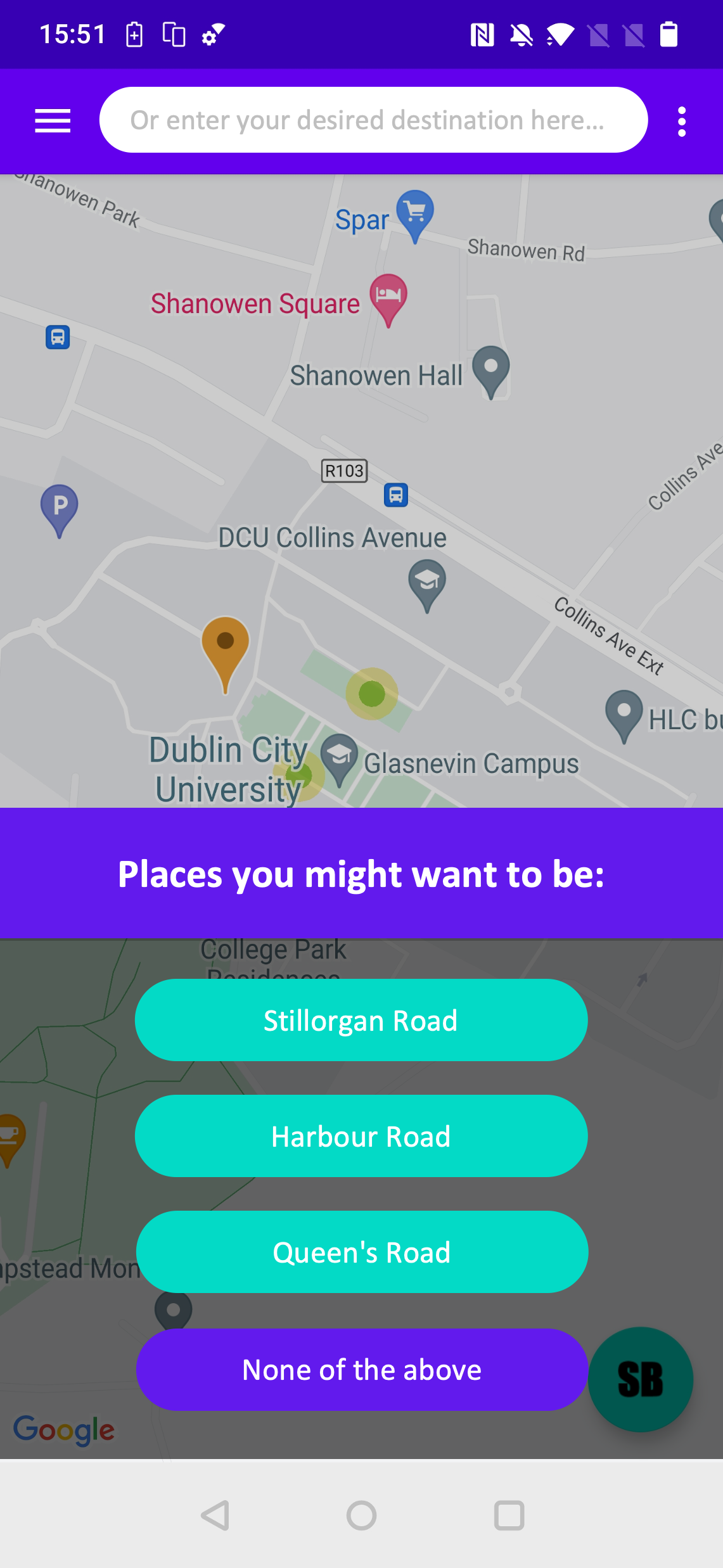
((a)) Pre-journey recommendation.

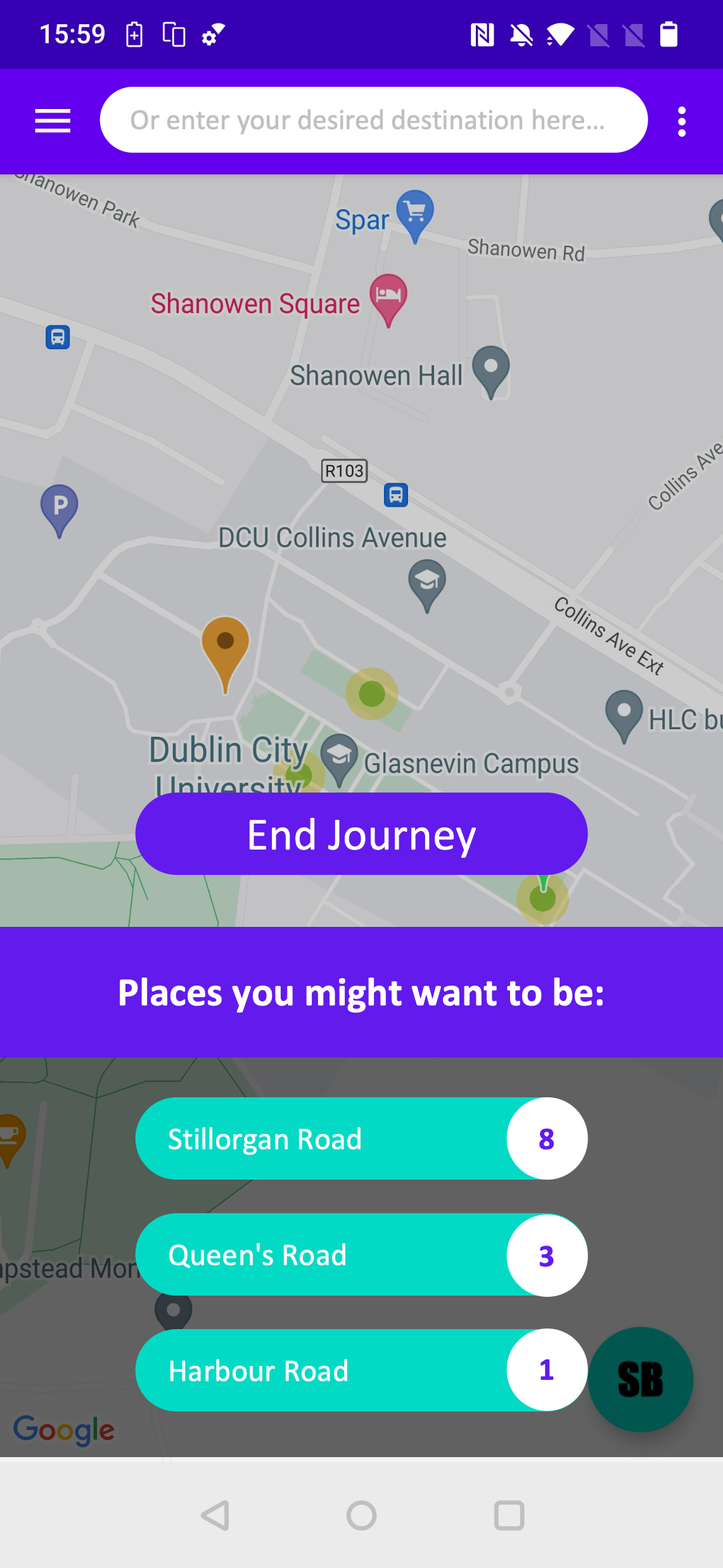
((b)) In-journey recommendation.

Figure 3: Sample user interfaces of recommendations.

Case 2: If all of the predicted results in $\mathbb{D}_{H}^{k}$ are different to $d_{U}^{k}$ (i.e., $\forall d_{x}\in\mathbb{D}_{H}^{k}$ $d_{x}\neq d_{U}^{k}$) or if the user ignores the recommendation in this stage, we denote this case by $d_{U}^{k}\notin\mathbb{D}_{H}^{k}$ and the system will estimate the expected value of the deposit based on the user’s previous destinations $\mathbb{D}$ and move to the in-journey stage. To do this, we define $\mathbb{D}_{k}$ as the set of destinations of all trips in the user’s historical record starting from the origin $p_{1}^{k}$, so $\mathbb{D}_{k}\subset\mathbb{D}$. Let $D_{k}$ denote the number of elements in $\mathbb{D}_{p_{1}^{k}}$, so $D_{k}\leq D$. For any destination $d_{l}^{k}\in\mathbb{D}_{k}$, the arrival timestamp is represented by $t_{l}^{k}$. We use $N_{l}$ to denote the number of all trips starting at $p_{1}^{k}$, and $N_{l}^{k}$ to denote the number of trips starting at $p_{1}^{k}$ and ending at $d_{l}^{k}$, so the weight of destination $d_{l}^{k}$ could be calculated by

$$w_{l}^{k}=\frac{N_{l}^{k}}{N_{l}}\qquad$$ (9)

where $w_{l}^{k}$ is the weight of $d_{l}^{k}$, then we know $\sum_{l=1}^{D_{k}}w_{l}^{k}=1$. Thus, the deposit for trip $\mathbb{T}_{k}$ is determined by the timestamps arriving at all destinations in $\mathbb{D}_{k}$ and the corresponding weights.

To sum up, the equation for deposit calculation is given by

$$F_{deposit}=\begin{cases}f\cdot(t_{U}^{k}-t_{1}^{k})&\text{if $d_{U}^{k}\in{\mathbb{D}^{k}_{H}}$}\\ f\cdot\sum_{l=1}^{D_{k}}w_{l}^{k}\cdot(t_{l}^{k}-t_{1}^{k})&\text{if $d_{U}^{k}\notin{\mathbb{D}^{k}_{H}}$}\end{cases}$$ (10)

where $f$ is the same constant value used in (8) representing the charge per second.

IV-C2 In-journey

In this stage, the GPS coordinates of the E-bike would be tracked and used to predict the destination of the current trip. As the trip $\mathbb{T}_{k}$ goes on, the trip trajectory will provide more spatial information about this trip. Our system will continuously recommend the predicted trip destination $d_{G}^{k}$ with a specific frequency, and save the prediction history in a list $\mathbb{D}_{G}^{k}$ which is sorted by the number of item occurrences. The user is allowed to select recommendation frequency and make the confirmation anytime, or they could also ignore the recommendations when cycling on the road, but when the user decides to end the current the journey and pay for the bill, the end journey command will be sent by clicking the corresponding button in our mobile application. Similarly, depending on the responses from users, three cases need to be considered in this step.

Case 1: If any predicted result $d_{y}$ in $\mathbb{D}_{G}^{k}$ is the same as $d_{U}^{k}$ (i.e., $\exists d_{y}\in\mathbb{D}_{G}^{k}$ $d_{y}=d_{U}^{k}$) and the user confirms it by selecting it from the list given in our mobile app, e.g., in Fig. 3(b), we denote this case by $d_{U}^{k}\in\mathbb{D}_{G}^{k}$ and our prediction module will adopt $d_{U}^{k}$ as the final result (i.e., $\hat{d}_{k}\leftarrow d_{U}^{k}$) and move to the post-journey stage without any further destination prediction.

Case 2: If the user ignores all the recommendations and is not ready to end the trip, we denote this case by $\nexists d_{U}^{k}$. The system will use the result at the top of $\mathbb{D}_{G}^{k}$ For example, a set of predicted destinations followed by the number their occurrence in Fig. 3(b). the interim result for this phase due to its highest occurrence value. Then, U-Park will begin the post-journey stage but continue tracking the user’s response towards the results made by this model till an end command is issued.

Case 3: If the user did not choose any predicted destination but is ready to end the trip by clicking the “End Journey” button shown in Fig. 3(b), we denote this case by $d_{U}^{k}\notin\mathbb{D}_{G}^{k}$. Then the user’s current location $p_{-1}^{k}$ will be set to the final result (i.e., $\hat{d}_{k}\leftarrow p_{-1}^{k}$) and move to the post-journey stage.

According to the explanation above, the full workflow of our destination prediction module is demonstrated in Algorithm 1. Important modules in the algorithm are $HistoryBasedModel$ (as introduced previously), $TrajectoryBasedModel$ (as introduced above) and $UserStop$ which indicates if the user’s trip is ending the trip.

Algorithm 1 Workflow of destination predictions

0:  An ongoing trip $\mathbb{T}_{k}=[(t_{1}^{k},p_{1}^{k});\dots]$, extra features $f_{k}$, distance threshold $dis$, (user-planned destination $d_{U}^{k}$)

0:  Prediction of destination $\hat{d_{k}}$

  if $d_{U}^{k}$ is initially given then

     $\hat{d_{k}}\leftarrow d_{U}^{k}$

     return  $\hat{d_{k}}$

  end if

  while length$(\mathbb{T}_{k})=1$ do

     $\mathbb{D}_{H}^{k}\leftarrow$ HistoryBasedModel$(\mathbb{T}_{k})$

     if $\exists d_{x}\in\mathbb{D}_{H}^{k}$ $d_{x}=d_{U}^{k}$ (i.e., $d_{U}^{k}\in\mathbb{D}_{H}^{k}$) then

        $\hat{d_{k}}\leftarrow d_{x}$

        return  $\hat{d_{k}}$

     end if

     wait for more trip data to be added

  end while

  while (UserStop$(\mathbb{T}_{k})=False$) & ($\hat{d_{k}}=nothing$) do

     $\mathbb{D}_{G}^{k}$ = TrajectoryBasedModel($\mathbb{T}_{k}$)

     if $\exists d_{y}\in\mathbb{D}_{G}^{k}$ $d_{y}=d_{U}^{k}$ then

        $\hat{d_{k}}\leftarrow d_{y}$

        return  $\hat{d_{k}}$

     else if UserStop$(\mathbb{T}_{k})=True$ then

        $\hat{d_{k}}\leftarrow p_{-1}^{k}$

        return  $\hat{d_{k}}$

     end if

  end while

IV-C3 Post-journey

With a destination confirmed by the user or predicted by U-Park, when the bike’s location becomes close enough to the final result of the trip destination $\hat{d}$ predicted by U-Park (i.e., less than $dis$ metres), our final prediction module will predict the parking space availability of a group of stations around $\hat{d}$ based on journey attributes (i.e., destination location, weather conditions and the approximate arrival time which is estimated by the map API). The prediction results represent available parking docks or space, so they would be used to determine the feasibility of recommending the user to park in this station or not. For instance, if any result is more than 5, which means there might be more than 5 parking positions available for this user when he or she arrives at the destination, with an MAE less than 1 [29], we would be more confident to recommend the user to park at this station because it will not be very difficult for this user to park in the proper position or zone.

On the other hand, if one result is less than 2 for example, the user is likely unable to find a parking position in his or her decided destination. In this case, U-Park will find some “available stations” based on the prediction results of stations around. The definition of “available stations” is described below. For a station $s_{u}$, only if its parking space availability $E_{u}$ is larger than a predefined threshold $E$, it could be regarded as an “available station”. Now with an example shown in Fig. 4, we demonstrate the process of parking station $\hat{s_{k}}$ determination as follows, which is decided by a probability distribution of the predicted results mentioned above.

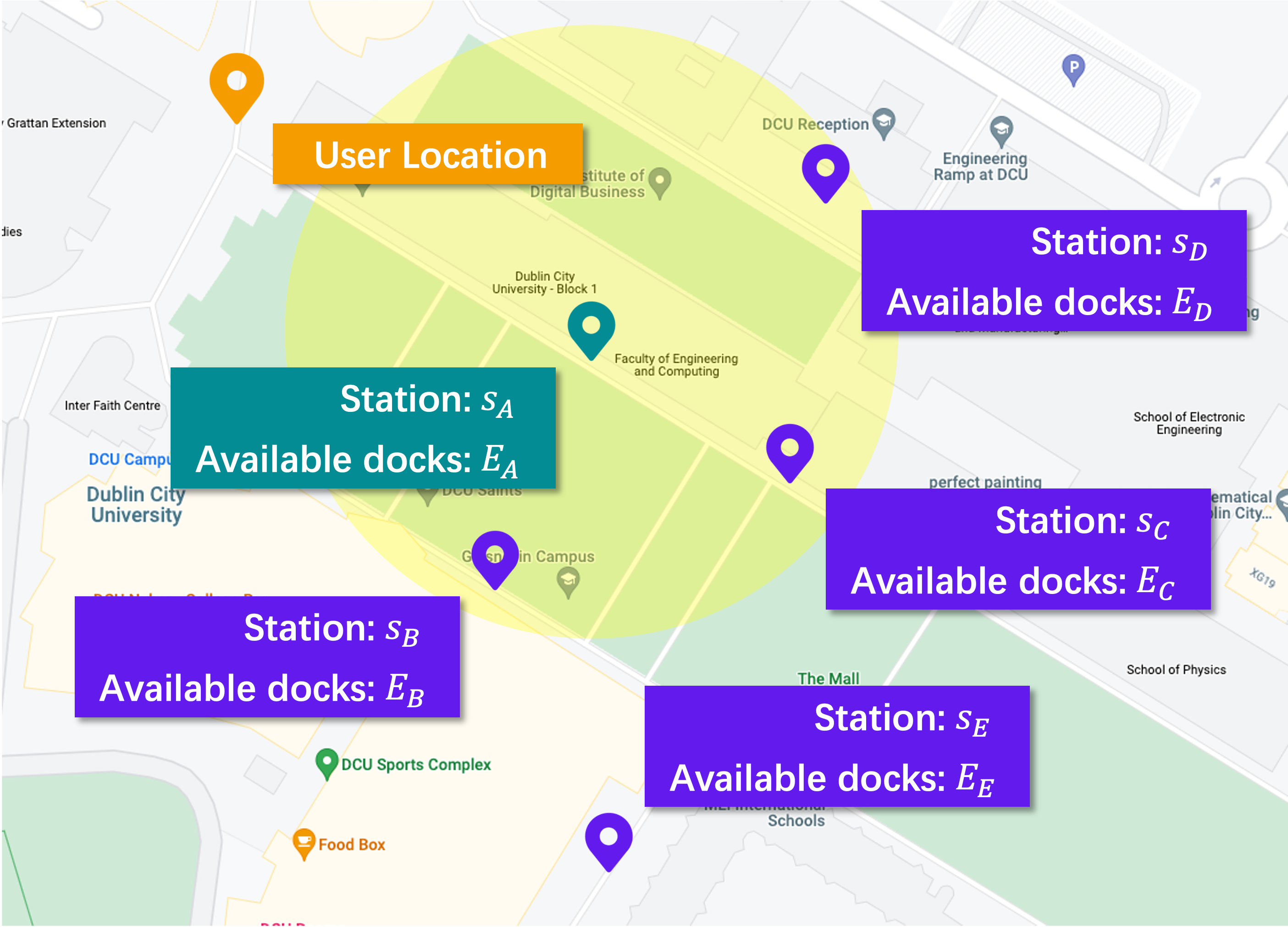
Figure 4: Parking station determination.

In the scenario shown in Fig. 4, Station $s_{A}$ represents the parking station at $\hat{d}$, of which the available parking space is $E_{\hat{d}}=E_{A}$. Stations $s_{B}$, $s_{C}$ and $s_{D}$ are the closest available stations to Station $s_{A}$ (i.e., in the region of the yellow circle with a radius of $m$ metres), while Station $s_{E}$ is outside the region, so it will not be used in decision making. Mathematically, we have $\forall E_{v}>E$ where Station $s_{v}\in\{s_{B},s_{C},s_{D}\}$. In this example, we assume $E_{A}<E$, which means Station $s_{A}$ is an unavailable station. Thus, the parking station recommended to the user will be determined by only Stations $s_{B}$, $s_{C}$ and $s_{D}$, and accordingly, the probability of Station $s_{v}$ being recommended to this user could be calculated by (11). For example, the probability of Station $s_{C}$ being recommended to the user, in this case, is $P_{C}=E_{C}/(E_{B}+E_{C}+E_{D})$.

$$P_{v}=\frac{E_{v}}{E_{B}+E_{C}+E_{D}}\qquad\text{$v\in\{B,C,D\}$}$$ (11)

The parking station recommendation method based on the probability works better than simply advising every cyclist with the same destination to park at Station $s_{v}$ because it avoids the change of the parking availability at Station $s_{v}$ in a very short time caused by the same recommendations. On the contrary, it balances the parking space in the region with a specific area.

IV-D Trading Module & Database

In the blockchain-based trading module, each user is added as a node to generate a peer-to-peer network, enabling interactions between users. A crypto wallet connects the web application and mobile application to the blockchain network. A smart contract is responsible for executing and managing blockchain operations, and a decentralised file storage system is applied to ensure that the decentralised web application can be implemented to allow the administrators to monitor and control financial transactions and operations. An overview of the interactions involving the trading module is shown in Fig. 5.

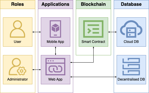
Figure 5: Workflow of trading module.

Precisely, at the beginning of a trip, our trading module will charge the user for the trip deposit based on the prediction result from our prediction module, and then at the end of this trip, the user will be charged the balance regarding the duration of the trip and the parking behaviour, e.g., their friendly behaviours and efforts, users parking their E-bikes at the suggested stations will be rewarded with a voucher or bonus, of which the process is implemented by the blockchain module.

The database would be used to store data collected from the hardware, user interface and trading modules, enabling these sections to interact with each other. Thus, we use a decentralised database to interact with our web application and a cloud database to store other data, for example, a table stored in our cloud database for transmitting data such as vehicle speed.

V System Implementation

We have implemented the proposed system, U-Park, for a shared E-bike system as a use case, so in this section, we introduce and present the implementation.

V-A Hardware Module

The hardware section is implemented by various sensors connected to the E-bike via a Raspberry Pi 3 Model B, which is a centralised controller capable of processing the physical status information of the E-bike captured by the sensors, such as GPS time series and digital lock status. Afterwards, the GPS time series, which is required by our prediction module, will be transferred to our database and the digital lock status will be used for interactions between the mobile application and the Raspberry Pi to lock or unlock an E-bike. Specifically, in our work, the geographic location of the E-bike is identified by a GPS module (i.e., the NEO-6M module) and the axial position of the E-bike is captured by the MPU6050 gyroscope and accelerometer module.

V-B User Interface Module

Our Android mobile application was developed on IntelliJ IDEA and then installed and tested on an $OnePlus$ $7pro$ with a processor of $Snapdragon^{TM}$ $855$. The interactive map was implemented with Google Maps API. It demonstrates the locations of the user and E-bikes as well as the stations predefined in terms of their exact parking areas with circles and parking availability with digits in real-time. In Fig. 6, the orange marker represents the user’s current location, obtained by the mobile application with Android locating service, and the green marker shows the current location of an E-bike. Circular areas filled with different colours define parking zones with different parking fees and the digit in each parking zone denotes its current parking availability. Regarding the GPS localisation accuracy at different regions (e.g., better performances in open areas), the size of parking zones will be scaled accordingly.

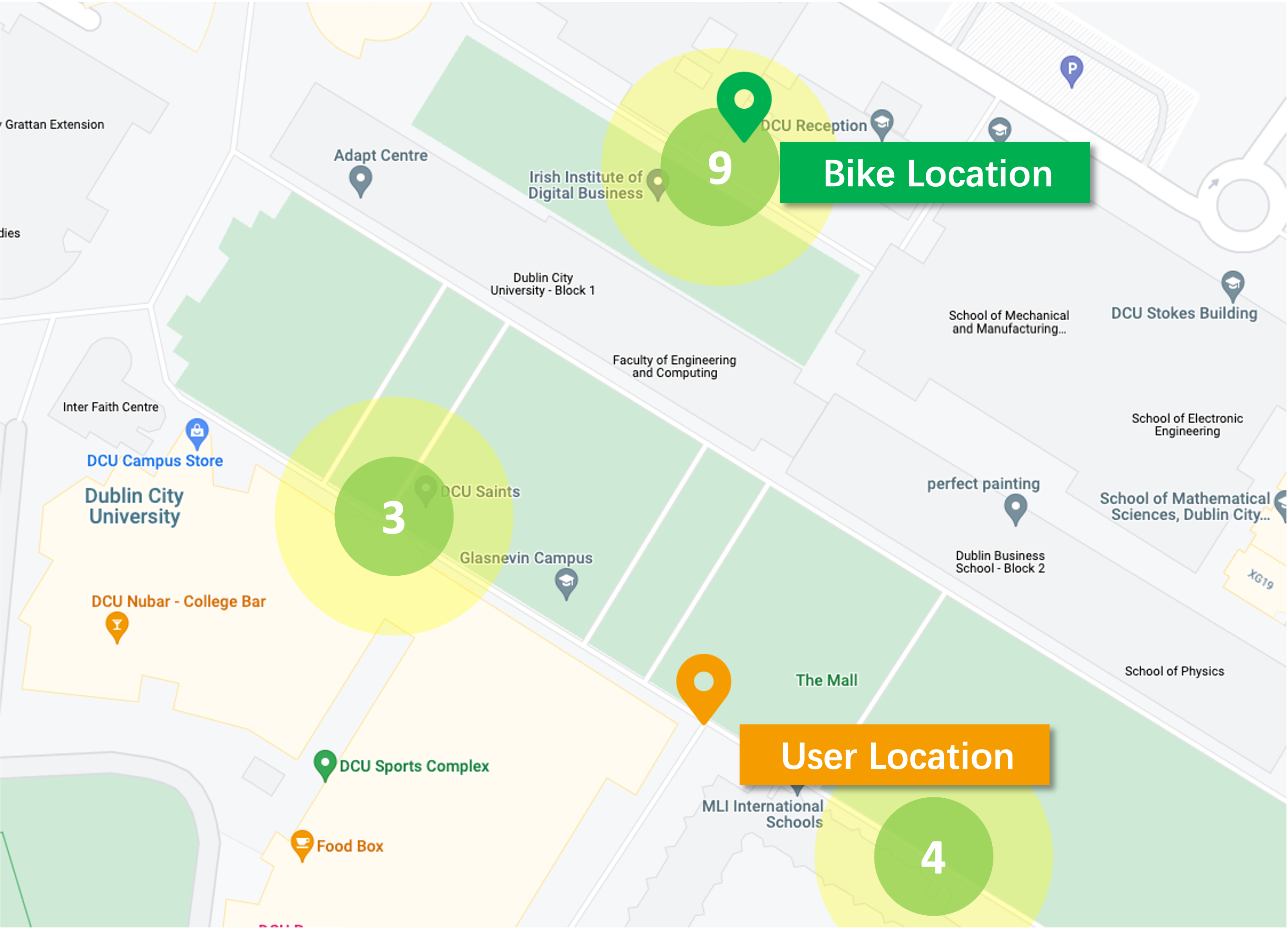
Figure 6: User location, E-bike position and pre-defined parking zones.

The QR code scanning function was implemented by the ZXing library. The scanning result contains the vehicle’s unique identification number (UID), GPS coordinate and current timestamp. The E-bike UID will be used for management and maintenance while the others will be sent to our prediction module to predict the destination which will be recommended to the user for confirmation and to examine whether the remaining battery capacity of this E-bike is enough for the predicted trip accordingly. If not, U-Park will wait for the user’s response to the predicted destination and recommend the user another E-bike which is the closest one with enough remaining battery capacity when the user confirms the journey destination. On the contrary, if the remaining batter capacity is enough for the predicted trip, the predicted destination will be used to calculate the deposit for this trip according to the method introduced above. Then, the calculated deposit and the user’s real-time credit would be transmitted to the smart contract for validation.

Data transmission with the smart contract was completed based on Web3j API. Besides, interactions with DynamoDB were implemented based on Amplify framework provided by AmazonWeb Services (AWS), which enabled us to create, read, update and delete items easily in our DB. The payment currency is U-Park Token (UPT), a cryptographic token developed for the app. Payments are processed through the integration of the mobile application with the Metamask SDK, a blockchain-based non-custodial wallet. Users can self-authenticate payments with security features, such as personal identification numbers (PINs).

To test our mobile application and hardware, we used DynamoDB to store the collected data. The GPS data collected from the hardware module consists of multiple trips with four universal attributes – trip ID, latitude, longitude, and timestamp, but when the user decides to stop this trip, four extra features would be attached to the last GPS coordinates (i.e., moving duration, moving fee, minimum distance to stations, and parking fee). This will enable us to verify the deposit and balance for this trip. Extracting the spatial and temporal features of the departure and arrival points (i.e., rental and return timestamps and GPS coordinates), we convert the collected GPS data to trip records followed by additional physical features mentioned above (i.e., moving duration, moving fee, minimum distance to stations, and parking fee). A statistical description of this dataset could be viewed in Table IV below.

TABLE IV: Statistical description of test trip report collected.

Object	Rental Lat	Rental Lon	Return Lat	Return Lon	Moving Duration (s)	Moving Fee	Parking Distance (m)	Parking Fee
mean	53.385287	-6.256454	53.385310	-6.256497	83.50	0.002505	36.16	0.063636
std	0.000595	0.001158	0.000600	0.001090	89.32	0.002680	33.27	0.041352
min	53.384259	-6.258351	53.384397	-6.258282	11.00	0.000330	1.94	0.000000
25%	53.384754	-6.257242	53.384616	-6.257286	24.00	0.000720	10.61	0.050000
50%	53.385542	-6.255965	53.385451	-6.256396	30.50	0.000915	20.35	0.075000
75%	53.385696	-6.255455	53.385707	-6.255468	112.50	0.003375	56.75	0.100000
max	53.386412	-6.254772	53.386556	-6.255093	318.00	0.009540	95.19	0.100000

V-C Trading Module & Database

The blockchain module aims to manage the logic of the financial transactions, a smart contract is developed with the Solidity and deployed on Ethereum’s Ropsten test network via Alchemy for validation. A decentralised Web3 application is developed using React JSX and Tailwind CSS, which enables the administrators to check and operate the information of any user or E-bike. The web application shown in Fig. 7 serves two main purposes: monitoring the status of the cycles, along with the incorporated sensor data, and facilitating the UPT transfer to the users on a top-up request. It is integrated with Metamask to enable crypto transactions, and upon receiving the users’ top-up request, the web application sends the requested UPT value to the user’s wallet address.

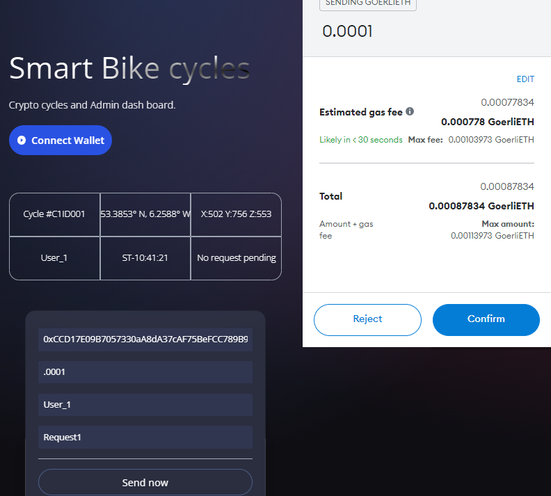
Figure 7: Prediction module workflow.

According to the incentive and punishment policy we introduced in Section II, the parking fee $F_{parking}$ mentioned in Section IV and applied in U-Park is determined by a tiered fee approach, as shown in (12).

$$F_{parking}=\begin{cases}0&\text{$D_{min}\leq D_{1}$}\\ 0.5\times F_{penalty}&\text{$D_{1}<D_{min}\leq D_{2}$}\\ F_{penalty}&\text{$D_{min}>D_{2}$}\end{cases}$$ (12)

where $D_{1}$ and $D_{2}$ are two distance thresholds and $D_{min}$ represents the minimum distance in metres to all stations, which is calculated by the E-bike’s current GPS location and the stations’ GPS locations. $F_{penalty}$ is the fine for failing to park the E-bike appropriately.

As concluded in [38], the mean walking speed for women aged 80 to 99 years is 0.943 metres per second (i.e., 56.58 metres per minute), which is the lowest mean speed among survey participants. Accordingly, 0.2 euros (i.e., 1.43 yuan in [33]) could be an acceptable reward for moving 50 metres. Regarding the potential influence of the users’ heterogeneous characteristics mentioned above, we decided to set $D_{1}$ and $D_{2}$ to 50 and 100 metres at this stage as an example, which will lead to punishment in user credits corresponding to 0.2 euros or 0.4 euros respectively. In other words, if users park the E-bikes within the inner circular zones marked with green in Fig. 6, it means for this journey, $D_{min}<50$, so $F_{parking}$ for this trip will be 0. Similarly, parking within the outer circular zones which are marked with yellow, the user will be charged half of the penalty and charged a full penalty if parking outside these zones.

In the aspect of the database, a distributed database based on InterPlanetary File System (IPFS) is adopted in the Web application to manage users’ credits, while DynamoDB is used to store and retrieve the data collected by sensors on E-bikes. Data collected in our test process include 22 trip records with 1384 points in total, but as a dataset for training a machine learning model, it is not very appropriate due to the small amount of data. Thus, we adopted another dataset, which is introduced in detail in the next section.

V-D Dataset and Preprocessing

The dataset from the shared E-bike company, MOBY, was used to examine the performance of the models proposed in this paper. A detailed description of the original dataset can be found in [1]. In this stage, we focused on a single user in our dataset whose trip pattern is more regular and representative. This user had 103 journey records with complete GPS coordinates collected during the trip. The analysis of his or her trip data revealed that there were 18 departure and 9 arrival stations among these 103 trips, with the two most frequently used stations being 215 and 261. These findings indicate the spatial regularity of this user’s travel mode, while in the aspect of temporal attributes, we found this user used the E-bike more frequently on Fridays and Saturdays and usually started from 2:00 pm to 5:00 pm and ended from 3:00 pm to 6:00 pm. Features used in our system includes the labels of the trip origin and destination, starting time (i.e., rental time), hourly rental demand at starting station (derived from statistics), and weather condition (i.e., precipitation amount, air temperature, wet bulb temperature, dew point temperature, vapour pressure, mean sea level pressure) collected from the Irish Meteorological Service.

Before the implementation of models, we split the feature Starting Time according to the hour and weekday, and with respect to GDPR, we then transformed the GPS information into road segment data, which only contain the road labels but not the exact GPS coordinates, by Mapbox Map Matching API. It is also worth mentioning that a significant imbalance in journey starting and ending points has been found for this user. For example, the imbalance in the number of trips starting from each station category led to weaker performance of our prediction module, so the algorithm SMOTE (i.e., Synthetic Minority Over-sampling Technique) [39] was used to address this issue by oversampling. Specifically, SMOTE calculates the $K$ nearest neighbours of each minority class sample, then randomly selects $N$ samples from the $K$ nearest neighbours for random linear interpolation, and constructs a new minority class sample accordingly. Finally, a new training set is generated by synthesising the new samples with the original data. After applying the SMOTE algorithm, more samples in minority categories are generated and added to our training set to solve the imbalance problem mentioned before. The modified dataset is shown in Table V, based on which machine learning models have been designed, implemented and evaluated.

TABLE V: Sample data of trip records from the modified dataset.

Return ID	Rental ID	Rental weekday	Rental hour	Hourly rentals	PA	AT	WBT	DPT	VP	MSLP	Road segment
215	199	1	16	2	0.0	21.0	18.4	16.7	19.1	1019.2	…, Stillorgan Road, …
215	214	5	14	2	0.0	5.9	4.7	3.1	7.6	1009.6	…, Stillorgan Road, …
261	261	0	20	2	0.0	13.5	7.9	0.1	6.2	1016.9	…, Queen’s Road, …
217	261	5	19	1	0.0	9.5	7.5	5.1	8.8	1006.8	…, Harbour Road, …
261	210	2	13	1	0.0	18.4	14.8	12.0	13.9	1024.8	…, Idrone Lane, …

• PA – Precipitation Amount (mm), AT – Air Temperature (C), WBT – Wet Bulb Temperature (C), DPT – Dew Point Temperature (C), VP – Vapour Pressure (hPa), MSLP – Mean Sea Level Pressure (hPa).

V-E Prediction Module

As mentioned in Section IV, our prediction module consists of three individual stages – destination prediction based on trip history, destination prediction based on partial trajectory, and parking space availability prediction based on station history, and each prediction task would be addressed by various machine learning models.

V-E1 History-Based Destination Prediction

The dataset used in this model is split into training data, validation data and test data with a ratio of 8:1:1, and a basic neural network model is implemented with two hidden layers with 64 and 32 units respectively and one dropout layer between them. The number of units in each layer is evaluated and tuned by the Hyperband algorithm [40], and they might be different when applied to other users’ trip records. More details about the model are shown in Table VI. We use Categorical Cross Entropy (CCE) as the loss function and Categorical Top-3 and Top-1 Accuracy as the metrics to evaluate the performance. Different combinations of features have been tested on the model to simulate the absence of certain features. The feature sets adopted in our work are as follows: (1) rental location ID (Init); (2) rental hourly demand (D); (3) rental hour and rental weekday (T); (4) precipitation amount, air temperature, wet bulb temperature, dew point temperature, vapour pressure, and mean sea level pressure (W).

TABLE VI: History-based model structure.

Layer Type	Output Shape	Param #
Input	[(None, 27)]	0
Dense	(None, 64)	1792
Dropout	(None, 64)	0
Dense	(None, 32)	2080
Dense	(None, 6)	198

V-E2 Trajectory-Based Destination Prediction

Based on road segments transformed from the partial trajectory, we split the dataset into training data, validation data and test data with a ratio of 8:1:1, and trained several models to predict the destination candidate.

Simple RNN: A simple RNN model is implemented with a structure shown in Table VII, including a dense layer with 64 units, a dropout layer and a dense layer with 32 units.

Attention-Based RNN: An attention-based RNN model is implemented with a structure shown in Table VIII, including a dense layer with 64 units, a Bahdanau attention layer, a dropout layer and a dense layer with 32 units.

LSTM: An LSTM model is implemented with a structure shown in Table IX, including an LSTM layer with 128 units, a dropout layer and a dense layer with 32 units.

Attention-Based LSTM: An attention-based LSTM model is implemented with a structure shown in Table X, including an LSTM layer with 128 units, a Bahdanau attention layer, a dropout layer and a dense layer with 32 units.

TABLE VII: Trajectory-based simple RNN model structure.

Layer Type	Output Shape	Param #
InputLayer	[(None, 10, 9)]	0
SimpleRNN	(None, 64)	4736
Dropout	(None, 64)	0
Dense	(None, 32)	2080
Dense	(None, 12)	396

TABLE VIII: Trajectory-based attention-based RNN model structure.

Layer Type	Output Shape	Param #
InputLayer	[(None, 10, 9)]	0
SimpleRNN	(None, 64)	4736
Attention	(None, 64)	74
Dropout	(None, 64)	0
Dense	(None, 32)	2080
Dense	(None, 12)	396

TABLE IX: Trajectory-based simple LSTM model structure.

Layer Type	Output Shape	Param #
InputLayer	[(None, 10, 9)]	0
LSTM	(None, 128)	70656
Dropout	(None, 128)	0
Dense	(None, 32)	4128
Dense	(None, 12)	396

TABLE X: Trajectory-based attention-based LSTM model structure.

Layer Type	Output Shape	Param #
InputLayer	[(None, 10, 9)]	0
LSTM	(None, 128)	70656
Attention	(None, 128)	138
Dropout	(None, 128)	0
Dense	(None, 32)	2080
Dense	(None, 12)	396

Again, the number of units in each layer is also evaluated and tuned by the Hyperband algorithm. Specifically, for a specific trip with a length of $L_{k}>(50+10-1)$, we randomly generated 50 numbers smaller than $(L_{k}-5)$ and accordingly intercepted 50 samples starting from the trip origin. For each segment, we only use the first 5 and the last 5 road segments to produce a sub-trajectory for this trip. For instance, for a trip $\mathbb{T}_{k}$ of which the length is 70, we generate 50 numbers smaller than 70. If a generated random number is 20, we take the first 20 points (i.e., $[(t_{1}^{k},p_{1}^{k}),\dots,(t_{20}^{k},p_{20}^{k})]$) as one sample and only use the first 5 (i.e., $[(t_{1}^{k},p_{1}^{k}),\dots,(t_{5}^{k},p_{5}^{k})]$) and last 5 points (i.e., $[(t_{16}^{k},p_{16}^{k}),\dots,(t_{20}^{k},p_{20}^{k})]$) to produce a sub-trajectory for this trip with a generated random number 20. The number of trips suitable for this prediction task is 46 for the selected user, so we obtained 2,300 sub-trajectories containing the first five and last five road segment labels. Again, we tested different combinations of features for this model, the initial feature combination (Init) is only a serial of road segment labels, and then we added temporal attributes (T) and weather conditions (W) as features. We use CCE as the loss function and Categorical Accuracy as the metric to evaluate the performance.

V-E3 Parking Space Availability Prediction

In [29], an Attention-based STGCN (ASTGCN) model has been proposed to predict the number of available shared bikes at different stands. The experiment results demonstrated the approach’s superiority compared to other existing methods in two datasets. An ASTGCN model with a structure similar to the one introduced in [29] will be implemented in our work. The number of available parking spaces at each parking station in the first several hours (e.g., 3 hours) will be adopted to predict parking space availability at each station at a certain time which is estimated by Google Maps API (e.g., 15 minutes later). The dataset will also be split for model training and the Mean Absolute Error (MAE) will be used as the performance metric to evaluate the performance across different models.

VI Results & Discussions

According to the description above, CCE was adopted as the error in both history-based and trajectory-based destination prediction models. Categorical Top-1 and Top-3 Accuracy were used as the evaluation metrics for the history-based basic neural network model, while only Categorical Top-1 Accuracy was adopted in our trajectory-based models (i.e., Simple RNN, AB-RNN, LSTM and AB-LSTM).

VI-A Feature Selection

Different feature combinations have been introduced in the previous section. In order to minimize the influence of random factors, we evaluated the performance of each combination 10 times and recorded the mean value of each metric in Table XI and Table XII.

VI-A1 History-Based Prediction Model

As shown in Table XI the model with only temporal and weather-relevant features performed best in both the loss (CCE) and the Top-3 Accuracy (around 97%) and compared with the initial input, the Top-3 and Top-1 Accuracy increased by around 11% and 31% respectively. The performance in Top-1 Accuracy is the highest (around 67%) when the input includes only demand and weather-relevant attributes, but it does not perform best in the Top-3 Accuracy (i.e., 91%). Thus, we consider the combination of rental location ID (Init), rental hour and rental weekday (T), and weather-relevant features (W) to have the best performance in this case study.

TABLE XI: History-based results with different features.

Features	CCE	Top-3 Accuracy	Top-1 Accuracy
Init	1.6008	0.86	0.33
Init+D	1.4866	0.91	0.41
Init+T	1.6701	0.96	0.44
Init+W	1.6670	0.90	0.62
Init+D+T	1.6161	0.91	0.45
Init+D+W	1.2218	0.91	0.67
Init+T+W	1.1242	0.97	0.64
Init+D+T+W	1.3518	0.93	0.66

• Items marked in bold are the best-preformed ones. Notations: Init - rental location ID only; D - rental hourly demand; T - rental hour and rental weekday; W - precipitation amount, air temperature, wet bulb temperature, dew point temperature, vapour pressure and mean sea level pressure.

VI-A2 Trajectory-Based Prediction Model

The performance of the trajectory-based model with different feature combinations is shown in Table XII. As the table shows, adding the temporal and weather-relevant attributes increased the accuracy by around 8.26% and 7.6% respectively compared with the initial attribute (i.e., only road segment labels). The combination of the all-attribute-included model is not the best but indicates less loss (CCE). Compared with the best Top-1 Accuracy produced by the history-based model (i.e., 67%), the trajectory-based model increases the prediction accuracy by around 30%. However, we did not find a very obvious improvement when the weather-relevant attributes were included in our trajectory-based model, so we suggest the combination of rental location ID (Init) and temporal attributes (T) performs best in this case study.

TABLE XII: Trajectory-based results with different features.

Features	CCE	Categorical Accuracy
Init	0.2136	0.8907
Init+T	0.0568	0.9733
Init+W	0.0585	0.9667
Init+T+W	0.0532	0.9720

• Items marked in bold are the best-preformed ones. Notations: Init - road segment label serial; T - rental hour and rental weekday; W - precipitation amount, air temperature, wet bulb temperature, dew point temperature, vapour pressure and mean sea level pressure.

To summarise, in the first two stages of our system, the trip destination is predicted by two different machine learning models, and the Top-1 accuracy of the output generated by our system increased from 60% in the first stage to more than $97\%$ in this stage with partial trajectory input.

VI-B Model Comparison for Trajectory-Based Prediction

In Table XIII, we compare and list trajectory-based models in different structures – Simple RNN, Attention-Based RNN (i.e., AB-RNN), LSTM and Attention-Based LSTM (i.e., AB-LSTM). It is obvious that without the attention layer, LSTM performs better than a Simple RNN model in both validation and test accuracy, but when the attention mechanism was applied, the AB-RNN model performs better than AB-LSTM and resulted in higher accuracy and less loss in both the validation and test set. Additionally, the AB-RNN model includes fewer parameters, which means the computational cost of model training smaller. Thus, we consider the AB-RNN model to be the best performer in this case study.

TABLE XIII: Trajectory-based results with different models.

Model	Val Loss	Val Acc	Test Loss	Test Acc	Params #
AB-LSTM	0.0912	0.9778	0.0886	0.9751	75,318
LSTM	0.0858	0.9733	0.0913	0.9720	75,180
AB-RNN	0.0517	0.9822	0.0496	0.9760	7,286
RNN	0.0604	0.9644	0.0562	0.9684	7,212

• Items marked in bold are the best preformed ones.

VII Limitations

The framework proposed in this paper is the first step towards making smart parking management for ESMS, but whilst our system has been tested on a real-world dataset it has not been trialled in a deployment setting. The prediction task in our last stage (i.e., parking space availability prediction) relies heavily on the data collected at shared E-bike stations, which was not available at the time of writing. The certainty and reliability of data are essential to our prediction work, but it is very difficult to obtain an open data source sufficiently comprehensive to provide detailed GPS time series and parking spaces at each stand.

On the other hand, with the growing popularity of the MaaS, more regular users will adopt our system. However, we currently only consider one user in this paper as a use case to illustrate the efficacy of U-Park. Besides, an automatic mechanism would be helpful to select the best model and the optimal hyperparameter for each user. Additionally, only very basic-structured models have been adopted in our work because other machine-learning models tend to overfit when applied to our dataset due to the small amount of data in our current dataset. With more comprehensive datasets and state-of-art machine-learning models, it is reasonable to believe that the performance of the recommendation system becomes better with our architecture proposed.

VIII Conclusion & Future Work

In this paper, we proposed the design of a smart parking management solution for ESMS, namely U-Park. We explained its architecture, which includes two prediction tasks in three stages, to help the customers park their shared E-bikes more properly by making recommendations. Regarding the prediction results of trip destinations in the first two stages, we increased the output accuracy from 60.00% to 97.33% by designing a partial trajectory-based AB-RNN model to dynamically correct the results of a trip history-based model. Based on the model used in parking space availability prediction, which was proposed in [29], we would be able to make further recommendations for their parking stations when the customers are about to complete their trips.

In the future, more state-of-art machine learning algorithms and well-structured models could be included in our system to improve its performance. We are also planning to examine our system on larger and more appropriate datasets, and if possible in real use in our industry.

References

- [1] S. Yan, M. Liu, and N. E. O'Connor, “Parking behaviour analysis of shared e-bike users based on a real-world dataset - a case study in dublin, ireland,” in 2022 IEEE 95th Vehicular Technology Conference: (VTC2022-Spring). IEEE, Jun. 2022.
- [2] M. McQueen, J. MacArthur, and C. Cherry, “The e-bike potential: Estimating regional e-bike impacts on greenhouse gas emissions,” Transportation Research Part D: Transport and Environment, vol. 87, p. 102482, Oct. 2020.
- [3] S. Cairns, F. Behrendt, D. Raffo, C. Beaumont, and C. Kiefer, “Electrically-assisted bikes: Potential impacts on travel behaviour,” Transportation Research Part A: Policy and Practice, vol. 103, pp. 327–342, Sep. 2017.
- [4] Y. Gu, M. Liu, M. Souza, and R. N. Shorten, “On the design of an intelligent speed advisory system for cyclists,” in 2018 21st International Conference on Intelligent Transportation Systems (ITSC). IEEE, Nov. 2018.
- [5] P. Astegiano, F. Fermi, and A. Martino, “Investigating the impact of e-bikes on modal share and greenhouse emissions: a system dynamic approach,” Transportation Research Procedia, vol. 37, pp. 163–170, 2019.
- [6] N.-F. Galatoulas, K. N. Genikomsakis, and C. S. Ioakimidis, “Spatio-temporal trends of e-bike sharing system deployment: A review in europe, north america and asia,” Sustainability, vol. 12, no. 11, p. 4611, Jun. 2020.
- [7] G. Dias, E. Arsenio, and P. Ribeiro, “The role of shared e-scooter systems in urban sustainability and resilience during the covid-19 mobility restrictions,” Sustainability, vol. 13, no. 13, p. 7084, Jun. 2021.
- [8] J. Morfeldt and D. J. A. Johansson, “Impacts of shared mobility on vehicle lifetimes and on the carbon footprint of electric vehicles,” Nature Communications, vol. 13, no. 1, Oct. 2022.
- [9] C. Shui and W. Szeto, “A review of bicycle-sharing service planning problems,” Transportation Research Part C: Emerging Technologies, vol. 117, p. 102648, Aug. 2020.
- [10] Z. Chen, D. van Lierop, and D. Ettema, “Dockless bike-sharing systems: what are the implications?” Transport Reviews, vol. 40, no. 3, pp. 333–353, Jan. 2020.
- [11] B. Cvijic, D. Pasalic, D. Bundalo, and Z. Bundalo, “Cloud based web application supporting vehicle toll payment system,” in 2016 5th Mediterranean Conference on Embedded Computing (MECO). IEEE, Jun. 2016.
- [12] A. Pandey, R. Khan, and A. K. Srivastava, “Challenges in automation of test cases for mobile payment apps,” in 2018 4th International Conference on Computational Intelligence & Communication Technology (CICT). IEEE, Feb. 2018.
- [13] A. Brown, N. J. Klein, and C. Thigpen, “Can you park your scooter there? why scooter riders mispark and what to do about it,” Findings, Feb. 2021.
- [14] S. Guidon, H. Becker, H. Dediu, and K. W. Axhausen, “Electric bicycle-sharing: A new competitor in the urban transportation market? an empirical analysis of transaction data,” Transportation Research Record: Journal of the Transportation Research Board, vol. 2673, no. 4, pp. 15–26, Mar. 2019.
- [15] X. Zhou, Y. Ji, Y. Yuan, F. Zhang, and Q. An, “Spatiotemporal characteristics analysis of commuting by shared electric bike: A case study of ningbo, china,” Journal of Cleaner Production, vol. 362, p. 132337, Aug. 2022.
- [16] N. Saum, S. Sugiura, and M. Piantanakulchai, “Short-term demand and volatility prediction of shared micro-mobility: a case study of e-scooter in thammasat university,” in 2020 Forum on Integrated and Sustainable Transportation Systems (FISTS). IEEE, Nov. 2020.
- [17] S. Phithakkitnukooon, K. Patanukhom, and M. G. Demissie, “Predicting spatiotemporal demand of dockless e-scooter sharing services with a masked fully convolutional network,” ISPRS International Journal of Geo-Information, vol. 10, no. 11, p. 773, Nov. 2021.
- [18] G. Xiao, R. Wang, C. Zhang, and A. Ni, “Demand prediction for a public bike sharing program based on spatio-temporal graph convolutional networks,” Multimed. Tools Appl., vol. 80, no. 15, pp. 22 907–22 925, Jun. 2021.
- [19] J. Luo, D. Zhou, Z. Han, G. Xiao, and Y. Tan, “Predicting travel demand of a docked bikesharing system based on LSGC-LSTM networks,” IEEE Access, vol. 9, pp. 92 189–92 203, 2021.
- [20] J. Lee and J. Kim, “Evaluation of spatial and temporal performance of deep learning models for travel demand forecasting: Application to bike-sharing demand forecasting,” Journal of Advanced Transportation, vol. 2022, pp. 1–13, Jun. 2022.
- [21] K. Boonjubut and H. Hasegawa, “Accuracy of hourly demand forecasting of micro mobility for effective rebalancing strategies,” Management Systems in Production Engineering, vol. 30, no. 3, pp. 246–252, Jul. 2022.
- [22] Y. Liu, R. Jia, X. Xie, and Z. Liu, “A two-stage destination prediction framework of shared bicycles based on geographical position recommendation,” IEEE Intelligent Transportation Systems Magazine, vol. 11, no. 1, pp. 42–47, 2019.
- [23] J. Jiang, F. Lin, J. Fan, H. Lv, and J. Wu, “A destination prediction network based on spatiotemporal data for bike-sharing,” Complexity, vol. 2019, pp. 1–14, Jan. 2019.
- [24] H. Miao, Y. Fei, S. Wang, F. Wang, and D. Wen, “Deep learning based origin-destination prediction via contextual information fusion,” Multimedia Tools and Applications, vol. 81, no. 9, pp. 12 029–12 045, Jan. 2021.
- [25] W. Wang, X. Zhao, Z. Gong, Z. Chen, N. Zhang, and W. Wei, “An attention-based deep learning framework for trip destination prediction of sharing bike,” IEEE Transactions on Intelligent Transportation Systems, vol. 22, no. 7, pp. 4601–4610, Jul. 2021.
- [26] F. Zong, Y. Tian, Y. He, J. Tang, and J. Lv, “Trip destination prediction based on multi-day GPS data,” Physica A: Statistical Mechanics and its Applications, vol. 515, pp. 258–269, Feb. 2019.
- [27] A. Nawaz, Z. Huang, and S. Wang, “SSMDL: Semi-supervised multi-task deep learning for transportation mode classification and path prediction with GPS trajectories,” in Web and Big Data. Springer International Publishing, 2020, pp. 391–405.
- [28] J. Liang, J. Tang, F. Liu, and Y. Wang, “Combining individual travel preferences into destination prediction: A multi-module deep learning network,” IEEE Transactions on Intelligent Transportation Systems, vol. 23, no. 8, pp. 13 782–13 793, Aug. 2022.
- [29] Z. Chen, H. Wu, N. E. O’Connor, and M. Liu, “A comparative study of using spatial-temporal graph convolutional networks for predicting availability in bike sharing schemes,” 2021.
- [30] J. P. Epperlein, J. Monteil, M. Liu, Y. Gu, S. Zhuk, and R. Shorten, “Bayesian classifier for route prediction with markov chains,” in 2018 21st International Conference on Intelligent Transportation Systems (ITSC). IEEE, Nov. 2018.
- [31] A. Brown, N. J. Klein, C. Thigpen, and N. Williams, “Impeding access: The frequency and characteristics of improper scooter, bike, and car parking,” Transportation Research Interdisciplinary Perspectives, vol. 4, p. 100099, Mar. 2020.
- [32] E. Heinen and R. Buehler, “Bicycle parking: a systematic review of scientific literature on parking behaviour, parking preferences, and their influence on cycling and travel behaviour,” Transport Reviews, vol. 39, no. 5, pp. 630–656, Mar. 2019.
- [33] L. Gao, Y. Ji, X. Yan, Y. Fan, and W. Guo, “Incentive measures to avoid the illegal parking of dockless shared bikes: the relationships among incentive forms, intensity and policy compliance,” Transportation, vol. 48, no. 2, pp. 1033–1060, Feb. 2020.
- [34] R. Chen, ““bike litter” and obligations of the platform operators: Lessons from china’s dockless sharing bikes,” Computer Law & Security Review, vol. 35, no. 5, p. 105317, 2019.
- [35] A. Rossi, G. Barlacchi, M. Bianchini, and B. Lepri, “Modelling taxi drivers’ behaviour for the next destination prediction,” IEEE Transactions on Intelligent Transportation Systems, vol. 21, no. 7, pp. 2980–2989, Jul. 2020.
- [36] J. Lv, Q. Sun, Q. Li, and L. Moreira-Matias, “Multi-scale and multi-scope convolutional neural networks for destination prediction of trajectories,” IEEE Transactions on Intelligent Transportation Systems, vol. 21, no. 8, pp. 3184–3195, Aug. 2020.
- [37] J. Tang, J. Liang, T. Yu, Y. Xiong, and G. Zeng, “Trip destination prediction based on a deep integration network by fusing multiple features from taxi trajectories,” IET Intelligent Transport Systems, vol. 15, no. 9, pp. 1131–1141, Jun. 2021.
- [38] R. W. Bohannon and A. W. Andrews, “Normal walking speed: a descriptive meta-analysis,” Physiotherapy, vol. 97, no. 3, pp. 182–189, Sep. 2011. [Online]. Available: https://doi.org/10.1016/j.physio.2010.12.004
- [39] N. V. Chawla, K. W. Bowyer, L. O. Hall, and W. P. Kegelmeyer, “SMOTE: Synthetic minority over-sampling technique,” Journal of Artificial Intelligence Research, vol. 16, pp. 321–357, Jun. 2002.
- [40] L. Li, K. Jamieson, G. DeSalvo, A. Rostamizadeh, and A. Talwalkar, “Hyperband: A novel bandit-based approach to hyperparameter optimization,” Journal of Machine Learning Research, vol. 18, no. 1, p. 6765–6816, jan 2017.