Critical Points and Convergence Analysis of Generative Deep Linear Networks Trained with Bures-Wasserstein Loss

Abstract

We consider a deep matrix factorization model of covariance matrices trained with the Bures-Wasserstein distance. While recent works have made advances in the study of the optimization problem for overparametrized low-rank matrix approximation, much emphasis has been placed on discriminative settings and the square loss. In contrast, our model considers another type of loss and connects with the generative setting. We characterize the critical points and minimizers of the Bures-Wasserstein distance over the space of rank-bounded matrices. The Hessian of this loss at low-rank matrices can theoretically blow up, which creates challenges to analyze convergence of gradient optimization methods. We establish convergence results for gradient flow using a smooth perturbative version of the loss as well as convergence results for finite step size gradient descent under certain assumptions on the initial weights.

1 Introduction

We investigate generative deep linear networks and their optimization using the Bures-Wasserstein distance. More precisely, we consider the problem of approximating a target Gaussian distribution with a deep linear neural network generator of Gaussian distributions by minimizing the Bures-Wasserstein distance. This problem is of interest in two ways. First, it pertains to the optimization of deep linear networks for a type of loss that is qualitatively different from the well-studied and very particular squared error loss. Second, it can be regarded as a simplified but instructive instance of the parameter optimization problem in generative networks, specifically Wasserstein generative adversarial networks, which are currently not as well understood as discriminative models.

The optimization landscapes and the properties of parameter optimization procedures for neural networks are among the most puzzling and actively studied topics in theoretical deep learning (see, e.g. Mei et al., 2018; Liu et al., 2022). Deep linear networks, i.e. neural networks having the identity as activation function, serve as simplified models for such investigations (Baldi & Hornik, 1989; Kawaguchi, 2016; Trager et al., 2020; Kohn et al., 2022; Bah et al., 2021). The study of linear networks has guided the development of several useful notions and intuitions in the theoretical analysis of neural networks, from the absence of bad local minima to the role of parametrization and overparametrization in gradient optimization (Arora et al., 2018, 2019a, 2019b). Many previous works have focused on discriminative or autoregressive settings and have emphasized the squared error loss. Although this loss is indeed a popular choice in regression tasks, it interacts in a very special way with the particular geometry of linear networks (Trager et al., 2020). The behavior of linear networks optimized with different losses has also been considered in several works (Laurent & Brecht, 2018; Lu & Kawaguchi, 2017; Trager et al., 2020) but is less well understood.

The Bures-Wasserstein distance was introduced by Bures (1969) to study Hermitian operators in quantum information, particularly density matrices. It induces a metric on the space of positive semi-definite matrices, and corresponds to the 2-Wasserstein distance between two centered Gaussian distributions (Bhatia et al., 2019). Wasserstein distances have several useful properties, e.g. they remain well defined between disjointly supported measures and have duality formulations (Villani, 2003) that allow for practical implementations. This makes them good candidates and indeed popular choices for learning generative models, with a well-known case being the Wasserstein Generative Adversarial Networks (WGANs) (Arjovsky et al., 2017). While the 1-Wasserstein distance has been most commonly used in this context, the Bures-Wasserstein distance has also attracted interest, e.g. in the works of Muzellec & Cuturi (2018); Chewi et al. (2020); Mallasto et al. (2022), and has also appeared in the context of linear quadratic Wasserstein generative adversarial networks (Feizi et al., 2020).

Notably, De Meulemeester et al. (2021) observed experimentally that the Bures-Wasserstein metric reduces the infamous problem of mode collapse in GANs. In particular, the authors reported improvements in mode coverage and generation quality by adding the Bures metric to the objective function of a GAN. Our work casts light on the theoretical properties of Bures-Wasserstein metric as a loss function to train deep linear generative neural networks, by studying a specific 2-Wasserstein GAN model.

A 2-Wasserstein GAN is a minimum 2-Wasserstein distance estimator expressed in Kantorovich duality (see details in Appendix B). This model can serve as a platform to develop the theory particularly when the inner problem can be solved in closed-form. Such a formula is available when comparing pairs of Gaussian distributions, in particular centered Gaussians, which corresponds precisely to the Bures-Wasserstein distance between the corresponding covariance matrices. Strikingly, even in this simple case, the properties of the corresponding optimization problem are not well understood; we aim to address this in the present work.

1.1 Contributions

We establish a series of results on the optimization of deep linear networks trained with the Bures-Wasserstein loss:

• We obtain an analogue of the Eckart-Young-Mirsky theorem characterizing the critical points and minimizers of the Bures-Wasserstein distance over matrices of a given rank (Theorem 4.2).

• To circumvent the non-smooth behaviour of the Bures-Wasserstein loss when the matrices drop rank, we introduce a smooth perturbative version (Definition 6 and Lemma 3.3), and characterize its critical points and minimizers over rank-constrained matrices (Theorem 4.5). Under some conditions on the function realization, we connect them to critical points on the parameter space (Proposition 4.6).

• For the Bures-Wasserstein loss and its smooth version, in Theorem 5.5 and Remark 5.6, we show exponential convergence of the gradient flow assuming balanced initial weights (Definition 2.1) and a modified margin deficiency condition (Definition 5.2).

• For the Bures-Wasserstein loss and its smooth version, in Theorem 5.7, we show convergence of gradient descent provided the step size is small enough and the initial weights are balanced.

1.2 Related works

Low rank matrix approximation

The function space of a linear network corresponds to $n\times m$ matrices of rank at most $\underline{d}$, the smallest width of the network. Hence optimization in the function space is closely related to the problem of approximating a given data matrix by a low-rank matrix. When the approximation error is measured in Frobenius norm, Eckart & Young (1936) characterized the optimal bounded-rank approximation of a given matrix in terms of its singular value decomposition. Mirsky (1960) obtained the same characterization for the more general case of unitary invariant matrix norms, which include the Euclidean operator norm and the Schatten-$p$ norms. There are further generalizations to certain weighted norms (Ruben & Zamir, 1979; Dutta & Li, 2017). However, for general norms the problem is known to be difficult (Song et al., 2017; Gillis & Vavasis, 2018; Gillis & Shitov, 2019).

Loss landscape of deep linear networks

For the squared error loss, the optimization landscape of linear networks has been studied in numerous works. The pioneering work of Baldi & Hornik (1989) focused on the two-layer case, and showed that there is a single minimum (up to a trivial parametrization symmetry) and all other critical points are saddle points. Kawaguchi (2016) obtained corresponding results for deep linear networks and showed the existence of bad saddles (with no negative Hessian eigenvalues) in parameter space for networks with more than three layers. Lu & Kawaguchi (2017) showed that if the loss is such that any local minimizer in parameter space can be perturbed to an equally good minimizer with full-rank factor matrices, then all local minimizers in parameter space are local minimizers in function space. Chulhee et al. (2018) found sets of parameters in which any critical point is a global minimizer, and any outside critical point is a saddle point. We also mention other works that study critical points for different types of neural network architectures, such as deep linear residual networks (Hardt & Ma, 2017) and deep linear convolutional networks (Kohn et al., 2022, 2023).

There are also several results for different losses. Laurent & Brecht (2018) showed that for deep linear nets with no bottlenecks all local minima are global for arbitrary convex differentiable losses. Trager et al. (2020) found that for linear networks with arbitrarily rank-constrained function space, the squared error loss is special in the sense that it ensures the non-existence of non-global local minima. However, for arbitrary convex losses, non-global local minimizers, when they exist, are always pure, meaning that they correspond to local minimizers in function space.

Optimization dynamics of deep linear networks

Saxe et al. (2014) studied the learning dynamics of deep linear networks under different types of initial conditions. Arora et al. (2019b) obtained a closed-form expression for the parametrization along time in a deep linear network for the squared error loss. Notably, the authors found that solutions with a lower rank are preferred as the depth of the network increases. Arora et al. (2018) derived several invariances of the flow and compared the dynamics in parameter and function spaces. For the squared error loss, Arora et al. (2019a) proved linear convergence of gradient descent for linear networks without bottlenecks, with weights initialized to fulfill two assumptions — approximate balancedness and so that the end-to-end matrix is close in some sense to the solution. We frame our discussion by similar assumptions. Under the balancedness assumption for the initial weights, Bah et al. (2021) showed that for deep linear neural networks, the gradient flow of the squared error loss can be cast as a Riemannian gradient flow in the function space, and as such converges to a critical point which is a global minimizer on the manifold of fixed rank matrices of a given rank. More recently, Nguegnang et al. (2021) extended this convergence analysis to the (full-batch) gradient descent algorithm.

As a last note, a detailed analysis of the dynamics in the case of shallow linear networks with the squared error loss was conducted by Tarmoun et al. (2021); Min et al. (2021). The authors use symmetric and asymmetric factorization of a shallow linear network to study its convergence dynamics. The role of the “imbalancedness” of the weights was also remarked in those works.

Bures-Wasserstein distance

The Bures-Wasserstein distance has been of particular interests due to its geometrical properties. Chewi et al. (2020) studied the convergence of gradient descent algorithms for the Bures-Wasserstein barycenter, proving linear rates of convergence. In contrast to our work, they considered a Polyak-Łojasiewicz inequality derived from optimal transport theory to circumvent the non geodesic convexity of the barycenter. In the same vein, Muzellec & Cuturi (2018) exploited optimal transport theory to optimize the distance between two elliptical distributions. To avoid rank deficiency, they perturbed the diagonal elements of the covariance matrix by a small parameter. We also mention that Feizi et al. (2020) characterized the optimal solution of a 2-Wasserstein GAN with a rank-$k$ linear generator as the $k$-PCA solution. We will obtain an analogous result in our particular parametrization, along with detailed descriptions of critical points.

1.3 Notations

We adopt the following notations. For any $n\in\mathbb{N}$, let $[n]:=\{1,2,\ldots,n\}$. We equip $\mathbb{R}^{n}$ with its usual inner product, and we denote by $\mathcal{O}(n)$ the space of real orthogonal matrices of size $n$. Let $\mathcal{S}(n)$ be the space of real symmetric matrices of size $n$. We denote $\mathcal{S}_{+}(n)$ (resp. $\mathcal{S}_{++}(n)$) the space of real symmetric positive semi-definite (resp. definite) matrices of size $n$. We use $\mathcal{M}(k;n,m)$ (resp. $\mathcal{M}(\leqslant k;n,m)$) to denote the set of matrices of size $n\times m$ with rank exactly $k$ (resp. at most $k$). If not specified, the size of the matrix is $n\times m$. The scalar product between two matrices $A,B\in\mathbb{R}^{n\times m}$ is $\langle A,B\rangle=\operatorname{tr}{A^{\top}B}$, and the associated Frobenius norm is $\|\cdot\|_{F}^{2}$. The identity matrix of size $n$ will be written as $I_{n}$, or $I$ when $n$ is clear. For a (Fréchet) differentiable function $f\colon X\to Y$, we denote its differential at $x\in X$ in the direction $v$ by $\operatorname{d\!}{}f(x)[v]$. Finally, $\operatorname{Crit}(f)$ is the set of critical points of $f$, i.e. the set of points at which the differential of $f$ is $0$.

2 Linear networks and their gradient dynamics

We consider a linear network with $d_{0}$ inputs and $N$ layers of widths $d_{1},\ldots,d_{N}$, which is a model of linear functions of the form

$$x\mapsto W_{N}\cdots W_{1}x,$$

parametrized by the weight matrices $W_{j}\in\mathbb{R}^{d_{j}\times d_{j-1}}$, for all $j\in[N]$. We will denote the tuple of weight matrices by $\overrightarrow{W}=(W_{1},\ldots,W_{N})$ and the space of all such tuples by $\Theta$. This is the parameter space of our model. To slightly simplify the notation we will also denote the input and output dimensions by $m\equiv d_{0}$ and $n\equiv d_{N}$, respectively, and write $W:=W_{N}\cdots W_{1}$ for the end-to-end matrix. For any $1\leqslant i\leqslant j\leqslant N$, we will also write $W_{j:i}:=W_{j}\cdots W_{i}$ for the matrix product of layer $i$ up to $j$. We note that the represented function is linear in the network input $x$, but the parametrization is not linear in the parameters $\overrightarrow{W}$. We denote the network’s parametrization map by

$$\mu\colon\Theta\to\mathbb{R}^{d_{N}\times d_{0}};\\ \overrightarrow{W}=(W_{1},\ldots,W_{N})\mapsto W_{N:1}=W_{N}\cdots W_{1}.$$

The function space of the network is the set of linear functions it can represent. This corresponds to the set of possible end-to-end matrices, which are the $n\times m$ matrices of rank at most $\underline{d}:=\min\{d_{0},\ldots,d_{N}\}$. When $\underline{d}=\min\{d_{0},d_{N}\}$, the function space is a vector space. Otherwise, when there is a bottleneck such that $\underline{d}<\min\{d_{0},d_{N}\}$, it is a non-convex subset of $\mathbb{R}^{m\times n}$ determined by polynomial constraints, namely the vanishing of the $(\underline{d}+1)\times(\underline{d}+1)$ minors.

Next, we collect a few results on the gradient dynamics of linear networks for general differentiable losses, which have been established in previous works with focus on the squared error loss (Kawaguchi, 2016; Bah et al., 2021; Chitour et al., 2022; Arora et al., 2018). In the interest of conciseness, here we only provide the main takeaways and defer a more detailed discussion to Appendix C. For the remainder of this section, let $\mathcal{L}^{1}\colon\mathbb{R}^{n\times m}\to\mathbb{R}$ be any differentiable loss and $\mathcal{L}^{N}$ be defined through the parametrization $\mu$ as $\mathcal{L}^{N}(\overrightarrow{W}):=\mathcal{L}^{1}\circ\mu(\overrightarrow{W})$. For such a loss, the gradient flow $t\mapsto\overrightarrow{W}(t)$ is defined by

$$\frac{\operatorname{d\!}}{\operatorname{d\!}t}\overrightarrow{W}(t) =-\nabla\mathcal{L}^{N}(\overrightarrow{W}(t))$$ (1)

$$\iff$$

$$\forall j\in[N],\quad\frac{\operatorname{d\!}}{\operatorname{d\!}t}W_{j}(t) =-\nabla_{W_{j}}\mathcal{L}^{N}(W_{1}(t),\ldots,W_{N}(t)).$$

This governs the evolution of the parameters. Furthermore, we observe that the partial derivative of $\mathcal{L}^{N}$ with respect to $W_{j}$, for all $j\in[N]$, is given by

$$\nabla_{W_{j}} \mathcal{L}^{N}(W_{1},\ldots,W_{N})$$ (2)

$$=W_{j+1}^{\top}\cdots W_{N}^{\top}\nabla\mathcal{L}^{1}(W)W_{1}^{\top}\cdots W_{j-1}^{\top}.$$

As it turns out, the gradient flow dynamics preserves the difference of the Gramians of subsequent layer weight matrices, which are thus invariants of the gradient flow; i.e.

$$\frac{\operatorname{d\!}}{\operatorname{d\!}t}(W_{j+1}(t)^{\top}W_{j+1}(t))=\frac{\operatorname{d\!}}{\operatorname{d\!}t}(W_{j}(t)W_{j}(t)^{\top}).$$

The notion of balancedness for the weights of linear networks was first introduced by Fukumizu (1998) in the shallow case and generalized to the deep case by Du et al. (2018). This is useful as it removes the redundancy of the parametrization when investigating the dynamics in function space and has been considered in numerous works.

Definition 2.1 (Balanced weights).

The weights $W_{1},\ldots,W_{N}$ are said to be balanced if, for all $j\in[N-1],~{}~{}W_{j}W_{j}^{\top}=W_{j+1}^{\top}W_{j+1}$.

Assuming balanced initial weights, if the flow of each $W_{j}$ is defined and bounded, then the rank of the end-to-end matrix $W$ remains constant during training (Bah et al., 2021, Proposition 4.4). Moreover, the products $W_{N:1}W_{N:1}^{\top}$ and $W_{N:1}^{\top}W_{N:1}$ can be written in a concise manner; namely, $W_{N:1}W_{N:1}^{\top}={(W_{N}W_{N}^{\top})}^{N}$ and $W_{N:1}^{\top}W_{N:1}={(W_{1}^{\top}W_{1})}^{N}$, which simplifies computations.

Remark 2.2.

Some attempts to relax the balanced initial weights assumption include the notion of approximate balancedness Arora et al. (2019a), which only requires that there exists $\delta>0$ such that $\|W_{j}W_{j}^{\top}-W_{j+1}^{\top}W_{j+1}\|_{F}\leqslant\delta$ for $j\in[N-1]$. Our proofs in this paper use exactly balanced initial weights for simplicity, but they would also work under the approximate balancedness setting. Further initializations have been proposed by e.g. Gidel et al. (2019); Yun et al. (2021). We defer the analysis of such cases for future work favoring here a focused discussion of the Bures-Wasserstein loss with balanced initial weights.

3 Wasserstein generative linear networks

3.1 The Bures-Wasserstein loss

The Bures-Wasserstein (BW) distance is defined on the space of positive semi-definite matrices (or covariance space) $\mathcal{S}_{+}(n)$. We collect definitions and key properties of the gradient.

Definition 3.1 (Bures-Wasserstein distance).

Given two symmetric positive semidefinite matrices $(\Sigma_{0},\,\Sigma)\in{(\mathcal{S}_{+}(n))}^{2}$, the squared Bures-Wasserstein distance between $\Sigma_{0}$ and $\Sigma$ is defined as

$$\mathcal{B}^{2}(\Sigma,\Sigma_{0})=\operatorname{tr}{\Big{(}\Sigma+\Sigma_{0}-2(\Sigma_{0}^{1/2}\Sigma\Sigma_{0}^{1/2})^{1/2}\Big{)}}.$$ (3)

Kroshnin et al. (2021, Lemma A.3) shows that the matrix square root is differentiable on the set of positive definite matrices. In turn, we can differentiate the BW distance at $\Sigma\in\mathcal{S}_{++}(n)$. However, the mapping $\Sigma\mapsto\mathcal{B}^{2}(\Sigma,\Sigma_{0})$ is not differentiable at all $n\times n$ matrices. Indeed, if we let $\Gamma Q\Gamma^{\top}$ be a spectral decomposition of $\Sigma_{0}^{1/2}\Sigma\Sigma_{0}^{1/2}$, then (3) can be written as

$$\mathcal{B}^{2}(\Sigma,\Sigma_{0})=\|\Sigma^{1/2}\|^{2}_{F}+\|\Sigma_{0}^{1/2}\|^{2}_{F}-2\operatorname{tr}{Q^{1/2}}.$$ (4)

Due to the square root on $Q$, the map $\Sigma\mapsto\mathcal{B}^{2}(\Sigma,\Sigma_{0})$ is not differentiable when the number of positive eigenvalues of $Q$, i.e. the rank of $\Sigma_{0}^{1/2}\Sigma\Sigma_{0}^{1/2}$, changes. More specifically, while one can compute the gradient over the set of matrices of rank $k$ for any given $k$, the norm of the gradient blows up if the matrix changes rank. We describe the gradient of $\mathcal{B}^{2}$ restricted to the set of full-rank matrices in Appendix B. We refer the reader to Bhatia et al. (2019) for further details on the BW distance.

3.2 Linear Wasserstein GAN

The distance defined in (3) corresponds to the 2-Wasserstein distance between two zero-centered Gaussians. It can be used as a loss for training models of Gaussian distributions, in particular generative linear networks. Recall that a zero-centered Gaussian distribution is completely specified by its covariance matrix. Given a bias-free linear network and a latent Gaussian distribution $\mathcal{N}(0,I_{m})$, a linear network generator computes a push-forward of the latent distribution, which is again a Gaussian distribution. If $Z\sim\mathcal{N}(0,I_{m})$ and $X=WZ$, then

$$X\sim\mathcal{N}(0,WW^{\top})=:\nu.$$

Given a target distribution $\nu_{0}=\mathcal{N}(0,\Sigma_{0})$ (or simply a covariance matrix $\Sigma_{0}$, which may be a sample covariance matrix), one can select $W$ by minimizing $\mathcal{B}^{2}(WW^{\top},\Sigma_{0})=\mathcal{W}_{2}^{2}(\nu,\nu_{0})$. We will denote the map that takes the end-to-end matrix $W$ to the covariance matrix $WW^{\top}$ by $\pi\colon\mathbb{R}^{n\times m}\to\mathbb{R}^{n\times n};\;W\mapsto WW^{\top}$.

Loss in covariance, function, and parameter spaces

We consider the following losses, which differ only on the choice of the search variable, taking either a covariance space, function space, or parameter space viewpoint.

• First, we denote the loss over covariance matrices $\Sigma\in\mathcal{S}_{+}(n)$ as $L\colon\Sigma\mapsto\mathcal{B}^{2}(\Sigma,\Sigma_{0})$.

• Secondly, given $\pi\colon W\mapsto WW^{\top}\in\mathcal{S}_{+}(n)$, we define the loss in the function space, i.e. over end-to-end matrices $W\in\mathbb{R}^{n\times m}$, as $L^{1}\colon W\mapsto L\circ\pi(W)$. This is given by, for $W\in\mathbb{R}^{n\times m}$,

  $$\quad L^{1}(W)=\operatorname{tr}{\Big{(}WW^{\top}+\Sigma_{0}-2(\Sigma_{0}^{1/2}WW^{\top}\Sigma_{0}^{1/2})^{1/2}\Big{)}}.$$ (5)

  This loss is not convex in $\mathbb{R}^{n\times m}$, which can be seen even in the scalar case.

• Lastly, for a tuple of weight matrices $\overrightarrow{W}=(W_{1},\ldots,W_{N})$, we compose $L^{1}$ with the parametrization map $\mu\colon\overrightarrow{W}\mapsto W_{N:1}$ to define the loss in the parameter space as $L^{N}\colon\overrightarrow{W}\mapsto L\circ\pi\circ\mu(\overrightarrow{W})$, for $\overrightarrow{W}\in\Theta$. Observe that this is, again, a non-convex loss.

Thus, for $\overrightarrow{W}\in\Theta$, $L^{N}(\overrightarrow{W})=L^{1}(\mu(\overrightarrow{W}))=L(\pi(\mu(\overrightarrow{W}))=\mathcal{B}^{2}(\pi\circ\mu(\overrightarrow{W}),\Sigma_{0})$. While the gradient flow (1) is defined on the parameters $\overrightarrow{W}$, viewing the problem in the covariance space is useful since then the objective function is convex, even if it may be subject to non-convex constraints. One of our goals is to translate properties between $L$, $L^{1}$, and $L^{N}$.

Smooth perturbative loss

As mentioned before, the Bures-Wasserstein loss is non-smooth at covariance matrices with vanishing eigenvalues. As a result, the usual analysis tools to prove uniqueness and convergence of the gradient flow do not apply here. To tackle this issue, we introduce a smooth perturbative version of the loss. Consider the perturbation map $\varphi_{\tau}\colon\Sigma\mapsto\Sigma+\tau I_{n}$, where $\tau>0$ plays the role of a regularization strength. Then the perturbative loss in the covariance space is defined as $L_{\tau}=L\circ\varphi_{\tau}$, and the perturbative loss in the function space as $L^{1}_{\tau}=L_{\tau}\circ\pi$. More explicitly, we let

$$L^{1}_{\tau}(W) =\operatorname{tr}\Big{(}WW^{\top}+\tau I_{n}+\Sigma_{0}$$ (6)

$$-2(\Sigma_{0}^{1/2}(WW^{\top}+\tau I_{n})\Sigma_{0}^{1/2})^{1/2}\Big{)}.$$

This function is smooth and allows us to apply usual convergence arguments for the gradient flow. Likewise, $L^{N}_{\tau}:=L_{\tau}\circ\pi\circ\mu$ is well-defined and smooth on $\Theta$.

Remark 3.2.

The perturbative loss (6), as well as the original loss on fixed-rank matrices, are differentiable. Many results of Bah et al. (2021) can be carried over for these differentiable Bures-Wasserstein losses. For example, the uniform boundedness at any time $t\geqslant 0$ of the end-to-end matrix holds, $\|W(t)\|\leqslant\sqrt{2L^{1}(W(0))+\operatorname{tr}\Sigma_{0}}$. Similar observations may apply for the case of $L^{1}$ in the case that the matrix $WW^{\top}$ remains positive definite throughout training, in which case the gradient flow remains well-defined and the loss is monotonically decreasing. We expand on this in Appendix C.

The next lemma, proved in Section B.4, provides a quantitative bound for the difference between the original and the perturbative loss. To compare the two losses, we set the parameters — and hence, the end-to-end matrices — to a fixed, common value.

Lemma 3.3.

Let $W\in\mathbb{R}^{n\times m}$ and $\tau>0$. Assume that $\operatorname{rank}{(\Sigma_{0})}=n$. Then, with $L^{1}(W)$ given by (5) and $L^{1}_{\tau}(W)$ given by (6), we have

$$|L^{1}_{\tau}(W)-L^{1}(W)|\leqslant n\sqrt{\tau}\left(\sqrt{\tau}+\frac{2\lambda_{\max}(\Sigma_{0}^{1/2})}{\lambda_{\min}(\Sigma_{0}^{1/2})}\right),$$ (7)

with $(\lambda_{\max}(\Sigma_{0}^{1/2}),\lambda_{\min}(\Sigma_{0}^{1/2}))$ the maximum and minimum eigenvalues of $\Sigma_{0}^{1/2}$.

We observe that the upper bound (7) is tight in $\tau$ in the sense that it goes to zero as $\tau$ goes to zero.

4 Critical points

In this section, we characterize the critical points of the Bures-Wasserstein loss restricted to matrices of a given rank. The proofs of results in this section are given in Appendix D.

For $k\in\mathbb{N}$, denote $\mathcal{M}(k)$ as the manifold of rank-$k$ matrices of size $n\times m$:

$$\mathcal{M}(k)\equiv\mathcal{M}(k;n,m):=\{W\in\mathbb{R}^{n\times m}\mid\operatorname{rank}{W}=k\}.$$ (8)

Similarly, we denote by $\mathcal{M}({\leqslant k})\equiv\mathcal{M}(\leqslant k;n,m)$ the set of $n\times m$ matrices of rank at most $k$. The manifold $\mathcal{M}(k)$ is an embedded submanifold of the linear space $(\mathbb{R}^{n\times m},\langle\cdot,\cdot\rangle_{F})$, with codimension $(n-k)(m-k)$ (Helmke & Shayman 1995, Proposition 4.5; Boumal 2022, §2.6). Given a function $f\colon\mathbb{R}^{n\times m}\to\mathbb{R}$, its restriction on $\mathcal{M}(k)$ is denoted by $f|_{\mathcal{M}(k)}\colon\mathcal{M}(k)\ni W\mapsto f(W)$. A function $f$ may not differentiable everywhere on $\mathbb{R}^{n\times m}$ but still have a restriction on $\mathcal{M}(k)$ that is differentiable.

Definition 4.1.

Let $\mathcal{M}$ be a smooth manifold. Let $f\colon\mathbb{R}^{n\times m}\to\mathbb{R}$ be any function such that its restriction on $\mathcal{M}$ is differentiable. A point $W\in\mathcal{M}$ is said to be a critical point of $f|_{\mathcal{M}}$ if the differential of $f|_{\mathcal{M}}$ at $W$ is the zero function, i.e. $\operatorname{d\!}{}f|_{\mathcal{M}}(W)=0$.

4.1 Critical points of $L^{1}$ over $\mathcal{M}(k)$

Given a matrix $A\in\mathbb{R}^{n\times n}$ and a set $\mathcal{J}_{k}\subseteq[n]$, where the subscript indicates the cardinality of the set, $k=|\mathcal{J}_{k}|$, we denote by $A_{\mathcal{J}_{k}}\in\mathbb{R}^{n\times k}$ the sub-matrix of $A$ consisting of the columns with index in $\mathcal{J}_{k}$. If the matrix $A$ is diagonal, we let $\bar{A}_{\mathcal{J}_{k}}\in\mathbb{R}^{k\times k}$ be the diagonal sub-matrix which extracts the rows and columns with index in $\mathcal{J}_{k}$. The following result characterizes the critical points of the loss in function space. It can be regarded as a type of Eckart-Young-Mirsky result for the case of the Bures-Wasserstein loss.

Theorem 4.2 (Critical points of $L^{1}$).

Assume $\Sigma_{0}$ has $n$ distinct, positive eigenvalues. Let $\Sigma_{0}=\Omega\Lambda\Omega^{\top}$ be a spectral decomposition of $\Sigma_{0}$ (so $\Omega\in\mathcal{O}(n)$), with eigenvalues ordered decreasingly. Let $k\in[\min\{n,m\}]$. A matrix $W^{*}\in\mathcal{M}(k)$ is a critical point of $L^{1}|_{\mathcal{M}(k)}$ if and only if $W^{*}=\Omega_{\mathcal{J}_{k}}\bar{\Lambda}_{\mathcal{J}_{k}}^{1/2}V^{\top}$ for some $\mathcal{J}_{k}\subseteq[n]$ with $|\mathcal{J}_{k}|=k$ and $V\in\mathbb{R}^{m\times k}$ with $V^{\top}V=I_{k}$. The minimum over $\mathcal{M}(\leqslant k)$ is attained precisely when $\mathcal{J}_{k}=[k]$. In particular, $\inf_{\mathcal{M}(k)}L^{1}(W)=\min_{\mathcal{M}(k)}L^{1}(W)$ and $\min_{\mathcal{M}(k)}L^{1}(W)=\min_{\mathcal{M}(\leqslant k)}L^{1}(W)$.

Remark 4.3.

Notice that there are $\binom{n}{k}$ critical points up to right rotation by an arbitrary orthonormal matrix (the trivial symmetry of $W\mapsto WW^{\top}$).

The proof relies on evaluating the zeros of the gradient $\nabla L^{1}|_{\mathcal{M}(k)}$ (see Lemma D.3). Then evaluating the loss at these critical points allows us to identify which of them attain the minimum.

Remark 4.4.

Interestingly, the critical points and the minimizer of $L^{1}$ characterized in the above result agree with those of the squared error loss (Eckart & Young, 1936; Mirsky, 1960). Nonetheless, we observe that (3) is only defined for positive semi-definite matrices. Hence the notion of unitary invariance considered by Mirsky (1960) only makes sense for left and right multiplication by the same matrix. Moreover, while we can establish unitary invariance for a variational expression of the distance (see Lemma 5.1), this is still not a norm in the sense that there is no function $B\colon\mathcal{S}_{+}(n)\to\mathbb{R}$ such that $\mathcal{B}(\Sigma,\Sigma_{0})=B(\Sigma-\Sigma_{0})$, and hence it does not fall into the framework of Mirsky (1960). We offer more details about this in Appendix B.

4.2 Critical points of the perturbative loss

For the critical points of the perturbative loss $L_{\tau}^{1}(W)$ we obtain the following results.

Theorem 4.5 (Critical points of $L^{1}_{\tau}$).

Assume $\Sigma_{0}$ has $n$ distinct, positive eigenvalues. Let $\Sigma_{0}=\Omega\Lambda\Omega^{\top}$ be a spectral decomposition of $\Sigma_{0}$, with eigenvalues ordered decreasingly. A point $W^{*}\in\mathcal{M}(k)$ is a critical point of $L^{1}_{\tau}|_{\mathcal{M}(k)}$ if and only if $W^{*}=\Omega_{\mathcal{J}_{k}}{(\bar{\Lambda}_{\mathcal{J}_{k}}-\tau I_{k})}^{1/2}V^{\top}$ for some $\mathcal{J}_{k}\subseteq[n]$ with $|\mathcal{J}_{k}|=k$ and $V\in\mathbb{R}^{n\times k}$ with $V^{\top}V=I_{k}$. Moreover, the value at such a point is $L^{1}_{\tau}(W^{*})=\sum_{j\not\in\mathcal{J}_{k}}(\sqrt{\lambda_{j}}-\sqrt{\tau})^{2}$. The minimum over $\mathcal{M}(\leqslant k)$ is therefore attained precisely when $\mathcal{J}_{k}=[k]$. In particular, $\inf_{\mathcal{M}(k)}L^{1}_{\tau}(W)=\min_{\mathcal{M}(k)}L^{1}_{\tau}(W)$ and $\min_{\mathcal{M}(k)}L^{1}_{\tau}(W)=\min_{\mathcal{M}(\leqslant k)}L^{1}_{\tau}(W)$.

Note that the above characterization of the critical points imposes an upper bound on $\tau$: for a given $W^{*}$ to be a critical point, one must have that $\tau\leq\lambda_{j}$ for all $j\in\mathcal{J}_{k}$, because the eigenvalues of $\bar{\Lambda}_{\mathcal{J}_{k}}-\tau I_{k}$ have to be nonnegative.

In order to link the critical points in the parameter space to the critical points in the function space, we appeal to the correspondence drawn by Trager et al. (2020, Propositions 6 and 7). For the Bures-Wasserstein loss, this allows to conclude the following.

Proposition 4.6 (Critical points in parameter space are critical points in function space).

Assume a full-rank target $\Sigma_{0}$ with spectral decomposition $\Sigma_{0}=\Omega\Lambda\Omega^{\top}$ and distinct eigenvalues $\lambda_{1}>\cdots>\lambda_{n}>0$ ordered decreasingly. Let $\tau\in(0,\lambda_{n}]$. If $\overrightarrow{W}^{*}\in\operatorname{Crit}(L^{N}_{\tau})$, then $W^{*}=\mu(\overrightarrow{W}^{*})$ is a critical point of the loss $L^{1}_{\tau}|_{\mathcal{M}(k)}$, where $k=\operatorname{rank}W^{*}$. Moreover, when $k=\underline{d}=\min_{i\in[N]}\{d_{i}\}$, then $\overrightarrow{W}$ is a local minimizer of the loss $L^{N}_{\tau}$ if and only if $W^{*}=\mu(\overrightarrow{W}^{*})$ is a local minimizer, and therefore the global minimizer, of $L^{1}_{\tau}|_{\mathcal{M}(\underline{d})}$. In this case, $\Sigma^{*}_{\tau}=W^{*}{W^{*}}^{\top}+\tau I_{n}$ is the $\tau$-best $\underline{d}$-rank approximation of the target in the covariance space, in the sense that $\Sigma^{*}_{\tau}=\Omega\begin{pmatrix}\Lambda_{[\underline{d}]}&\\ &\tau\end{pmatrix}\Omega^{\top}$.

Proposition 4.6 ensures that, under the assumption that the solution of the gradient flow is a (local) minimizer in the parameter space and has the highest possible rank $\underline{d}$ for the given network architecture, the solution in the covariance space is the best $\underline{d}$-rank approximation of the target in the sense of the $\tau$-smoothed Bures-Wasserstein distance. The fact that any local minimizer of $L^{1}_{\tau}|_{\mathcal{M}(\underline{d})}$ is indeed a global minimizer is not immediate (since neither the loss $L^{1}_{\tau}$ nor the set $\mathcal{M}(\underline{d})$ are convex), but can be shown as we do in Lemma D.10.

Remark 4.7.

Under the balancedness assumption, one can show that the rank of the end-to-end matrix does not drop during training (Bah et al., 2021, Proposition 4.4), and that the trajectory almost surely escapes the strict saddle points (Bah et al., 2021, Theorem 6.3). If the initialization of the network has rank $\underline{d}$, the matrices $W(t),\,t>0$, maintain rank $\underline{d}$ throughout training. There can be issues in the limit, since $\mathcal{M}(\underline{d})$ is not closed. Proving whether or not the limit point also belongs to $\mathcal{M}(\underline{d})$ is an interesting open problem.

5 Convergence analysis

The Bures-Wasserstein distance can be viewed through the lens of the Procrustes metric (Dryden et al., 2009; Masarotto et al., 2019). In fact, it can be obtained by the following minimization problem.

Lemma 5.1 (Bhatia et al. 2019, Theorem 1).

For $(\Sigma,\Sigma_{0})\in{(\mathcal{S}_{+}(n))}^{2}$,

$$\mathcal{B}^{2}(\Sigma,\Sigma_{0})=\min_{U\in\mathcal{O}(n)}\|\Sigma^{1/2}-\Sigma_{0}^{1/2}U\|_{F}^{2},$$ (9)

where $\mathcal{O}(n)$ denotes the set of $n\times n$ orthogonal matrices. Moreover, the minimizer $\bar{U}$ occurs in the polar decomposition of $\Sigma^{1/2}\Sigma_{0}^{1/2}$.

We emphasize that in the above description of the Bures-Wasserstein distance, the minimizer $\bar{U}$ depends on $W$, so that $\mathcal{B}^{2}$ fundamentally differs from a squared Frobenius norm. Moreover, the square root on $\Sigma$ can lead to singularities when differentiating the loss. Nonetheless, based on (9) we can formulate the following deficiency margin concept to avoid such singularities.

Definition 5.2 (Modified deficiency margin).

Given a target matrix $\Sigma_{0}\in\mathbb{R}^{n\times n}$ and a positive constant $c>0$, we say that $\Sigma\in\mathbb{R}^{n\times n}$ has a modified deficiency margin $c$ with respect to $\Sigma_{0}$ if

$$\min_{U\in\mathcal{O}(n)}\|\Sigma^{1/2}-\Sigma_{0}^{1/2}U\|_{F}\leqslant\sigma_{\min}(\Sigma_{0}^{1/2})-c.$$ (10)

With a slight abuse of terminology, we will say that $W$ has a modified deficiency margin if $WW^{\top}$ does. The deficiency margin idea can be traced back to Arora et al. (2019a). Note that we can write $\sqrt{WW^{\top}}=\Sigma^{1/2}$, and this square root can be realized by Cholesky decomposition. If we initialize the parameters so that $\Sigma$ is close to the target $\Sigma_{0}$, then (10) holds trivially. In fact, if the initial value $W(0)$ satisfies the modified deficiency margin condition, then the least singular value of $W(t)$ remains bounded below by $c$ along gradient flow or gradient descent trajectories with decreasing $L^{N}$:

Lemma 5.3.

Suppose $W(0)W(0)^{\top}$ has a modified deficiency margin $c$ with respect to $\Sigma_{0}$. Then

$$\sigma_{\min}\Big{(}\sqrt{W(t)W(t)^{\top}}\Big{)}\geqslant c,\quad~{}\text{for}~{}t\geqslant 0.$$ (11)

The proof of this and all results in this section are provided in Appendix E. We note that, while the modified deficiency margin assumption is sufficient for Lemma 5.3 to hold, it is by no means necessary. We will assume that the modified deficiency margin assumption holds for simplicity of exposition, but the gradient flow analysis in the next paragraph only requires the less restrictive Lemma 5.3 to hold.

5.1 Convergence of gradient flow for the smooth loss

Since we cannot exclude the possibility that the rank of $WW^{\top}$ drops along the gradient flow of the BW loss, we consider the smooth perturbation introduced in Section 3.2 as a way to avoid singularities. We consider the gradient flow (1) for the perturbative loss. The gradient of (6) is

$$\begin{split}&\nabla L^{1}_{\tau}(W)=\\ &2\Big{(}W-\Sigma_{0}^{1/2}\big{(}\Sigma_{0}^{1/2}(WW^{\top}+\tau I_{n})\Sigma_{0}^{1/2}\big{)}^{-1/2}\Sigma_{0}^{1/2}W\Big{)}.\end{split}$$

The perturbation $\tau I_{n}$ ensures that $\lambda_{\min}(\Sigma_{\tau})\geqslant\tau>0$, which in turn makes $L_{\tau}$ strongly-convex, as shown next.

Lemma 5.4.

The Hessian operator $\mathbb{G}_{\tau}$ of the loss $L_{\tau}$ at $\Sigma\in\mathcal{S}_{+}(n)$ satisfies $\lambda_{\min}(\mathbb{G}_{\tau})\geqslant K_{\tau}$ for any $\Sigma\in\mathcal{S}_{+}(n)$, with $K_{\tau}:=\frac{\sqrt{\tau\lambda_{\min}(\Sigma_{0})}}{2C_{\tau}^{2}}$, where $C_{\tau}:=2(L_{\tau}(\Sigma(0))+\operatorname{tr}{\Sigma_{0}})$.

This is proven in Lemma E.6.

Let us denote the minimizer of the perturbative loss $L(\Sigma_{\tau})$ by $\Sigma_{\tau}^{*}$. Equipped with the strong convexity of the loss $L_{\tau}$ given by Lemma 5.4, we are ready to show that the gradient flow has convergence rate $O(e^{-\tilde{K}_{c,N}K_{\tau}t})$ to the global minimizer of $L_{\tau}$, where $K_{\tau}$ is the constant from the Hessian bound given by Lemma 5.4, and $\tilde{K}_{c,N}$ is a constant which depends on the modified margin deficiency and the depth of the network. Recall that for $t\geqslant 0$, $\Sigma_{\tau}(t)=W_{N:1}(t)W^{\top}_{N:1}(t)+\tau I_{n}$, so we prove convergence of gradient flow on the loss under the parametrization $\Sigma_{\tau}(t)=\varphi_{\tau}(\pi(\mu(\overrightarrow{W}(t))))$.

Theorem 5.5 (Convergence of gradient flow for the smooth loss).

Let $\Delta_{\tau}^{*}:=\Sigma_{\tau}(0)-\Sigma_{\tau}^{*}$ be the distance from the initialization to the minimizer $\Sigma_{\tau}^{*}:=\operatorname*{arg\,min}_{\Sigma\in\mathcal{S}_{++}(n)}L_{\tau}(\Sigma)=\Sigma_{0}-\tau I_{n}$. Assume both balancedness (Definition 2.1) and the modified deficiency margin (Definition 5.2). Then the gradient flow $\dot{}\overrightarrow{W}(t)=-\nabla L^{N}_{\tau}(\overrightarrow{W}(t))$ converges as

$$L(\Sigma_{\tau}(t))-L(\Sigma_{\tau}^{*})\leqslant e^{-8Nc^{\frac{2(2N-1)}{N}}K_{\tau}t}\Delta_{\tau}^{*},$$ (12)

where $K_{\tau}=\frac{\sqrt{\tau\lambda_{\min}(\Sigma_{0})}}{2C_{\tau}^{2}}$ is the strong convexity parameter from Lemma 5.4, with $C_{\tau}=2(L(\Sigma_{\tau}(0))+\operatorname{tr}(\Sigma_{0}))$.

Remark 5.6.

Under the modified margin assumption (Definition 5.2), the parametrized covariance matrix $\Sigma=WW^{\top}$ has its eigenvalues lower-bounded by $c^{2}$ at all times, as per Lemma 5.3. Therefore, the convergence result obtained in Theorem 5.5 can be extended to the original loss, with $(\Sigma_{\tau}(t),\Sigma_{\tau}^{*})$ replaced with $(\Sigma(t),\Sigma^{*})$, $\Delta_{\tau}^{*}$ replaced with $\Delta^{*}:=\Sigma(0)-\Sigma^{*}$, $K_{\tau}$ replaced with $K_{c^{2}}=\frac{\sqrt{c^{2}\lambda_{\min}(\Sigma_{0})}}{2C^{2}}$, and $C_{\tau}$ replaced with $C_{0}=2(L(\Sigma(0))+\operatorname{tr}(\Sigma_{0}))$. More details about this are given in Section E.3.

5.2 Convergence of gradient descent for the BW loss

Assuming that the initial end-to-end matrix $W$ has a modified deficiency margin, we can establish the following convergence result for gradient descent with finite step sizes, which is valid for both the perturbed loss and the original (non-perturbed) loss. Given an initial value $\overrightarrow{W}(0)$, we consider the gradient descent iteration

$$\overrightarrow{W}(k+1)=\overrightarrow{W}(k)-\eta\nabla L^{N}(\overrightarrow{W}(k)),\quad k=0,1,\ldots,$$ (13)

where $\eta>0$ is the learning rate or step size and the gradient is given by (2).

Theorem 5.7 (Convergence of gradient descent).

Assume that the initial values $W_{i}(0)$, $1\leqslant i\leqslant N$, are balanced and $W(0)=W_{N:1}(0)$ has a modified deficiency margin $c$. If the learning rate $\eta>0$ satisfies

$$\eta\leqslant\min\left\{\frac{c^{2}}{8M\sqrt{L^{1}(W(0))}},~{}\frac{Nc^{\frac{2(N-1)}{N}}}{2\Delta},~{}\frac{1}{4Nc^{\frac{2(N-1)}{N}}}\right\},$$

where $\Delta=\frac{2^{N+1}}{c^{2N}}N^{2}M^{(4N-3)/N}\lambda^{1/2}_{\max}(\Sigma_{0})+8N(N-1)M^{(3N-4)/N}\Big{(}M^{1/N}+\|\Sigma_{0}^{1/2}\|_{F}\Big{)}$, and $M=\sqrt{2{L^{1}(W(0))+\|\Sigma_{0}^{1/2}\|^{2}_{F}}}$, then, for any $\epsilon>0$, one achieves $\epsilon$ loss by the gradient descent (13) at iteration

$$k\geqslant\frac{1}{2\eta Nc^{\frac{2(N-1)}{N}}}\log\left(\frac{L^{1}(W(0))}{\epsilon}\right).$$

Remark 5.8.

Theorems 5.5 and 5.7 show that the depth of the network can accelerate the convergence of the gradient algorithms. We verify this experimentally in Section 5.3.

5.3 Experimental evaluation of the convergence rate

We conduct numerical experiments to illustrate our theoretical results. We observe empirically (Figure 1) the linear dependency of the asymptotic rate of convergence as a function of the depth of the network $N$ and the minimum singular value square root of the target $\sigma_{\min}(\Sigma_{0}^{1/2})$.

Setup

The target covariance matrix is sampled as $\Sigma_{0}:=\Omega\Lambda\Omega^{\top}$, where $\Omega\in\mathbb{R}^{n\times n}$ is a random orthogonal matrix, and the eigenvalues in $\Lambda$ follow a Zipf distribution, $\lambda_{j}\propto{1}/{j}$ for $j\in[n]$. The input data dimension is set to be $n=20$. We vary the minimum eigenvalue for the target $\lambda_{\min}$ and set $\lambda_{j}=n/j\cdot\lambda_{\min}$ for $j\in[n]$. We consider constant width networks with $d_{i}=n=m=20$, for each $i\in[N]$.

To fulfill the modified deficiency margin assumption (Definition 5.2), we initialize the parameters close to the target $\Sigma_{0}$. If $\Sigma_{0}=\Omega\Lambda\Omega^{\top}$, then the weights are initialized in a way such that the initial covariance matrix is $\Sigma(0)=(\Sigma_{0}-\tau I_{n})+A$, with $A$ being a random perturbation. More precisely, we choose $A=\Gamma D\Gamma^{\top}$, where $\Gamma$ is a random orthogonal matrix, and $D$ is a diagonal matrix with small eigenvalues — so that the overall distance between the initialization and the target is bounded by $\sigma_{\min}-c$, for some $c>0$. With this initialization and the balancedness protocol explained by Arora et al. (2019a), the network satisfies both the balancedness and modified deficiency margin assumptions. In this case we expect Theorem 5.5 to hold for small step sizes. We estimate the asymptotic linear convergence rate numerically.

Result

We compute the rate of convergence as follows. First, the network (initialized as detailed above) is trained with a small enough learning rate $\eta$. Then, we compute $\log{(L(\Sigma(t)-L(\Sigma^{*})))}$. Theorem 5.5 states that this should be a linear function of the time $t$. Therefore, a linear regression is performed, and the slope taken as the empirical rate of convergence. According to Theorem 5.5, this rate should be linear in the depth $N$ and linear in the strong convexity parameter $K_{\tau}$, which suggests that it could be linear in $\sigma_{\min}(\Sigma_{0}^{1/2})\equiv\sigma_{\min}$. Hence, we compute the empirical rate of convergence for varying depths and $\sigma_{\min}$, reported in Figure 1. In Figure 1(a) the linear dependence in the depth is clearly visible, and Figure 1(b) indicates a linear dependence in $\sigma_{\min}$ too. Our Theorem 5.5 only provides an upper bound on the convergence rate and hence we compare with the empirical rates. The results suggest that this is indeed the actual behavior in practice.

(a)

(b)

Figure 1: Logarithm of the linear convergence rate as a function of the depth $N$ and the minimum singular value $\sigma_{\min}(\Sigma_{0}^{1/2})$. In (a), $\sigma_{\min}(\Sigma_{0}^{1/2})\approx 0.7078$ is fixed; convergence rate and its linear regression as a function of the depth $N$. In (b), both the depth and $\sigma_{\min}$ are varying, and the rate is shown in a contour plot. The hyperbolas indicate a linear dependency on both the depth $N$ of the network and the minimum singular value of the target square root $\sigma_{\min}(\Sigma_{0}^{1/2})$, which is coherent with the upper-bound given by Theorem 5.5.

6 Conclusion

In this work, we studied the training of generative linear neural networks using the Bures-Wasserstein distance. We characterized the critical points and minimizers of this loss in function space, over the set of matrices of fixed rank $k$. We introduced a smooth approximation of the BW loss, obtained by regularizing the covariance matrix, and characterized its critical points in function space as well. Furthermore, under the assumption of balanced initial weights satisfying a modified deficiency margin condition, we established a convergence guarantee to the global minimizer for the gradient flow of both losses, with exponential rate of convergence. Finally, we also considered the finite step-size gradient descent optimization and established a linear convergence result for both losses too, provided the step size is small enough depending on the modified deficiency margin condition. We collect our results in Tables 1 and 2 in Appendix A. These results contribute to the ongoing efforts to better characterize the optimization problems that arise in learning with deep neural networks beyond the commonly considered discriminative settings with the square loss.

In future work, it would be interesting to refine our characterization of critical points of the Bures-Wasserstein loss in the parameter space, and to relax the modified deficiency margin condition that we invoked in order to establish our convergence results, as this constrains the parametrization to be of full rank.

Acknowledgments

This project has been supported by DFG SPP 2298 grant 464109215, ERC Starting Grant 757983, and BMBF in DAAD project 57616814. GM has been supported by NSF CAREER 2145630 and NSF 2212520. We would like to warmly thank the anonymous reviewers for their questions and helpful comments.

Appendix

The appendix is organized as follows.

• Appendix A gives a quick summary of the different geometrical and convergence results.

• Appendix B provides background on the Bures-Wasserstein loss and related optimal transport topics.

• Appendix C presents general properties of linear neural networks and classical results on convergence in parameter space.

• Appendix D presents the proofs of results about critical points from Section 4.

• Appendix E presents the proofs of results about convergence from Section 5.

• Appendix F evaluates the Hessian of the loss.

Appendix A Summary of the results

Tables 1 and 2 present a summary of the results obtained in this paper.

Loss	Parametrization	Critical points	Ref
$L^{1}$	$W$	$\Omega_{\mathcal{J}_{k}}\bar{\Lambda}_{\mathcal{J}_{k}}^{1/2}V^{\top}$	Theorem 4.2
$L^{1}_{\tau}$	$W$	$\Omega_{\mathcal{J}_{k}}{(\bar{\Lambda}_{\mathcal{J}_{k}}-\tau I_{k})}^{1/2}V^{\top}$	Theorem 4.5

Table 1: Summary of critical point results. The target is assumed full rank with distinct eigenvalues and spectral decomposition $\Sigma_{0}=\Omega\Lambda\Omega^{\top}$. Here $V\in\mathbb{R}^{m\times k}$ is any semi-orthogonal matrix and $\mathcal{J}_{k}\subset[n]$ is an index set of cardinality $k$.

Loss	Parametrization	Initialization	Convergence rate	Ref
$L^{N}_{\tau}$	$\overrightarrow{W}$	Balanced, MDM	GF: Exponential	Theorem 5.5
$L^{N}$	$\overrightarrow{W}$	Balanced, MDM	GD: $O(\log(1/\epsilon))$	Theorem 5.7

Table 2: Summary of convergence results. Here “Balanced” stands for balanced weights (Definition 2.1), “MDM” stands for modified deficiency margin (Definition 5.2), and $\epsilon$ is the precision we want to achieve (Theorem 5.7).

Appendix B Properties of the Bures-Wasserstein distance

B.1 BW and the 2-Wasserstein distance

The Bures-Wasserstein distance has a natural connection with the 2-Wasserstein distance on a metric space. In the case of zero-centered Gaussian measures, the two distances are identical. We briefly describe the general definition of the 2-Wasserstein distance.

Given a metric space $(\mathcal{X},\|\cdot\|)$, the 2-Wasserstein distance is a well-known metric on the space of quadratically integrable probability measures $\mathcal{P}_{2}(\mathcal{X}):=\{\mu\in\mathcal{P}(\mathcal{X})\mid\int{\|x\|^{2}\operatorname{d\!}\mu(x)}<\infty\}$.

Definition B.1 (2-Wasserstein distance).

The 2-Wasserstein distance between two measures $(\nu,\nu_{0})\in{(\mathcal{P}_{2}(\mathcal{X}))}^{2}$ is defined as the solution to following minimization problem:

$$\mathcal{W}_{2}^{2}(\nu,\nu_{0})=\inf_{\pi\in\Pi(\nu,\nu_{0})}\int\|x-y\|^{2}\operatorname{d\!}\pi(x,y),$$ (14)

where $\Pi(\nu,\nu_{0})$ is the set of distributions with fixed marginals $\nu$ and $\nu_{0}$, $\Pi(\nu,\nu_{0})=\{\pi\in\mathcal{P}_{2}(\mathcal{X}\times\mathcal{X})\mid\pi_{1}=\nu,\,\pi_{2}=\nu_{0}\}$, with $\pi_{i}$ denoting the marginal of $\pi$ along the $i$th variable.

It is known that the 2-Wasserstein distance metrizes the weak convergence on the space $\mathcal{P}_{2}$ (see, e.g. Villani, 2008, Theorem 6.9). Therefore, it can used to compare probability distributions in systems such as GANs. On the other hand, the cost of computing this loss can quickly become prohibitive (see, e.g. Pele & Werman, 2009). Only in some cases, efficient ways to compute (14) are known. In a usual WGAN (Arjovsky et al., 2017), an approximation of the $1$-Wasserstein distance is computed based on the dual expression of the ($1$-)Wasserstein distance using a neural network to approximate the dual variable, called the discriminator network.

The 2-Wasserstein distance between two Gaussian measures has a closed-form expression (or a closed-form expression for the discriminator), so that adversarial training is not needed. We will consider two centered Gaussian distributions, which are described by their covariance matrices. In the case of centered Gaussian distributions, the 2-Wasserstein distance reduces to the Bures-Wasserstein distance between the covariance matrices $\Sigma_{0}$ and $\Sigma$ (Dowson & Landau, 1982):

Lemma B.2.

If $\nu=\mathcal{N}(\bm{m},\Sigma)$ and $\nu_{0}=\mathcal{N}(\bm{m}_{0},\Sigma_{0})$, then

$$\mathcal{W}_{2}^{2}(\nu,\nu_{0})=\|\bm{m}-\bm{m}_{0}\|^{2}+\mathcal{B}^{2}(\Sigma,\Sigma_{0}).$$

It is well known (see Kantorovitch 1958 or Villani 2003, Theorem 1.3 or Villani 2008, Theorem 5.10) that the squared 2-Wasserstein distance has the following dual expression, also known as the Kantorovich duality:

$$\begin{split}\mathcal{W}_{2}^{2}(\nu_{0},\nu_{\theta})=\sup_{(f,g)\in L^{1}(\nu_{\theta})\times L^{1}(\nu_{0})}&\Big{\{}\int{f(x)\operatorname{d\!}\nu_{\theta}(x)}+\int{g(x)\operatorname{d\!}\nu_{0}(x)}\mid\forall(x,y),\,f(x)+g(y)\leqslant\|x-y\|^{2}\Big{\}},\end{split}$$ (15)

where $L^{1}(\nu)$ is the set of the integrable functions with respect to a measure $\nu$. Therefore, the dual variables $f$ and $g$ are required to be integrable with respect to the source and target measures, and to fulfill the cost inequality.

Remark B.3.

In the context of WGANs it is common to consider the 1-Wasserstein distance with cost given by the distance $\|x-y\|$. This has a dual expression, referred to as the Kantorovich-Rubinstein formula (Villani, 2008, §6.2), that allows for a more tractable computation in practice, with for instance only one dual variable. Nonetheless, in general there is no closed-form solution known when $c(x,y)=\|x-y\|$.

B.2 BW and the Eckart-Young-Mirsky theorem

In this section, we provide further background on the Bures-Wasserstein distance. First, we show that, except in some particular cases (Lemma B.4), the Bures-Wasserstein distance between two covariance matrices is not translation invariant (Lemma B.5), which implies that it cannot be expressed as the norm (let alone unitary) of a difference between two matrices. Then, an explanation as to why the critical points found in Theorem 4.2 are the same as the one found when using the squared Frobenius norm between $\Sigma$ and $\Sigma_{0}$ is given.

Lemma B.4.

In the case that $\Sigma_{0}$ and $\Sigma$ commute, the Bures-Wasserstein distance reduces to the Hellinger distance:

$$\Sigma_{0}\Sigma=\Sigma\Sigma_{0}\quad\implies\quad\mathcal{B}^{2}(\Sigma,\Sigma_{0})=\|\Sigma^{1/2}-\Sigma_{0}^{1/2}\|_{F}^{2}.$$

Proof.

This follows from the fact that, if $\Sigma$ and $\Sigma_{0}$ commute, so do $\Sigma^{1/2}$ and $\Sigma_{0}^{1/2}$, so that $\Sigma_{0}^{1/2}\Sigma\Sigma_{0}^{1/2}={(\Sigma_{0}^{1/2}\Sigma^{1/2})}^{2}$ and

$$\operatorname{tr}{((\Sigma^{1/2})^{2}+(\Sigma_{0}^{1/2})^{2}-2{({\Sigma_{0}^{1/2}}{\Sigma^{1/2}})})} =\operatorname{tr}{({({\Sigma^{1/2}}-{\Sigma_{0}^{1/2}})}({\Sigma^{1/2}}-{\Sigma_{0}^{1/2}})^{\top})}$$

$$=\|{\Sigma^{1/2}}-{\Sigma_{0}^{1/2}}\|_{F}^{2},$$

as claimed. ∎

From this, one remarks that the problem of minimizing the BW distance between covariance matrices that commute falls under the framework of the Eckart-Young-Mirsky theorem. In this case if the optimization variable is $\Sigma^{1/2}={(WW^{\top})}^{1/2}$, we obtain a formulation in terms of the squared error loss. Nonetheless, in the case where $\Sigma$ and $\Sigma_{0}$ do not commute, we do not have such a correspondence, as in general, the BW distance is not translation invariant, neither when considered as a function of $(\Sigma,\Sigma_{0})$ nor when considered as a function of $(\Sigma^{1/2},\Sigma_{0}^{1/2})$.

Lemma B.5 (BW is not translation invariant).

There exist positive semidefinite matrices $(\Sigma,\Sigma_{0})\in\mathcal{S}_{+}(n)\times\mathcal{S}_{+}(n)$ and a translation $T\in\mathcal{S}_{+}(n)$, such that $\mathcal{B}^{2}(\Sigma+T,\Sigma_{0}+T)\neq\mathcal{B}^{2}(\Sigma,\Sigma_{0})$. The same statement also holds for the loss $\mathcal{E}$ defined on the matrix square roots, $\mathcal{E}(\Sigma^{1/2},\Sigma_{0}^{1/2}):=\mathcal{B}^{2}(\Sigma,\Sigma_{0})$.

Proof.

For the first part of the statement, taking

$$\Sigma=\begin{pmatrix}1&0\\ 0&1\end{pmatrix},\quad\Sigma_{0}=\begin{pmatrix}1&0\\ 0&2\end{pmatrix},\quad T=\begin{pmatrix}t&0\\ 0&t\end{pmatrix},\quad t>0,$$

then $\mathcal{B}^{2}(\Sigma+T,\Sigma_{0}+T)-\mathcal{B}^{2}(\Sigma,\Sigma_{0})={(\sqrt{2+t}-\sqrt{1+t})}^{2}-{(\sqrt{2}-1)}^{2}$, which is non-zero.

For the second part of the statement, if

$$\Sigma_{0}^{1/2}=\begin{pmatrix}1&0\\ 0&2\end{pmatrix},\quad\Sigma^{1/2}=\begin{pmatrix}1&1\\ 1&2\end{pmatrix},\quad T=\begin{pmatrix}1&0\\ 0&1\end{pmatrix},$$

one computes

$$\mathcal{E}(\Sigma^{1/2},\Sigma_{0}^{1/2})= \|\Sigma^{1/2}\|_{F}^{2}+\|\Sigma_{0}^{1/2}\|_{F}^{2}-2\operatorname{tr}{(\Sigma_{0}^{1/2}\Sigma\Sigma_{0}^{1/2})}^{1/2}$$

$$= 12-2\operatorname{tr}{\begin{pmatrix}2&6\\ 6&20\end{pmatrix}^{1/2}}$$

and

$$\mathcal{E}(\Sigma^{1/2}+T,\Sigma_{0}^{1/2}+T)= \|\Sigma^{1/2}+T\|_{F}^{2}+\|\Sigma_{0}^{1/2}+T\|_{F}^{2}$$

$$-2\operatorname{tr}{((\Sigma_{0}^{1/2}+T)(\Sigma^{1/2}+T)(\Sigma^{1/2}+T)(\Sigma_{0}^{1/2}+T))}^{1/2}$$

$$= 28-2\operatorname{tr}{\begin{pmatrix}20&30\\ 30&90\end{pmatrix}^{1/2}},$$

which gives the difference $\mathcal{E}(\Sigma^{1/2}+T,\Sigma_{0}^{1/2}+T)-\mathcal{E}(\Sigma^{1/2},\Sigma_{0}^{1/2})\approx 0.121229\neq 0$. ∎

Lemma B.5 implies that in general one cannot express the Bures-Wasserstein distance (either on the covariance or on their square roots) as a norm of a difference (otherwise, the loss would be translation invariant). This hinders a direct application of the Eckart-Young-Mirsky theorem, where the problem is cast as $\min_{X}\|A-X\|_{*}$ with a fixed $A$ for some unitary invariant norm $\|\cdot\|_{*}$.

Nonetheless, there is a close link between the Bures-Wasserstein distance and the (squared) Euclidean distance. This is best seen through the definition of the 2-Wasserstein distance between two zero-centered Gaussian distributions, as we will present next. We follow here an approach inspired by Feizi et al. (2020, Theorem 1), for which we provide details in order to show a link between the minimization of the Bures-Wasserstein distance over rank-constrained covariance matrices and the Eckart-Young-Mirsky theorem (or $k$-PCA).

Given $k\in[n]$, the set of rank-$k$ positive semi-definite matrices is denoted by $\mathcal{S}_{+}(k;n)$. With $n\in\mathbb{N}\setminus\{0\}$ and $k\in[n]$, we are interested in the minimization problem

$$\inf_{A\in\mathcal{S}_{+}(k;n)}\mathcal{B}^{2}(A,B).$$ (16)

For any measure $\alpha$, denote $\operatorname{supp}(\alpha)$ its support, i.e. $\alpha(X)=0$ for $X\subseteq\mathbb{R}^{n}\setminus\operatorname{supp}(\alpha)$. The following is a well known connection between covariance matrices and the support of the corresponding Gaussian probability distributions.

Lemma B.6.

Let $A\in\mathcal{S}_{+}(k;n)$ and $\alpha=\mathcal{N}(0,A)$. Then the support of $\alpha$ is equal to the column space of $A$,

$$\operatorname{supp}(\alpha)=\operatorname{span}(A).$$

For $k\in[n]$, denote the set of linear subspaces of $\mathbb{R}^{n}$ of dimension $k$ by $\mathfrak{L}(\mathbb{R}^{n},k)$, and, for $\mathcal{C}\in\mathfrak{L}(\mathbb{R}^{n},k)$, denote by $\mathcal{N}(\mathcal{C}):=\{\mathcal{N}(0,M)\mid M\in\mathcal{S}_{+}(k;n),\,\operatorname{span}(M)=\mathcal{C}\}$ the set of all Gaussian distributions with mean $0$ and support $\mathcal{C}$.

Lemma B.6 allows to translate the problem (16) to a problem on linear subspaces of fixed dimension. Indeed, with $\alpha=\mathcal{N}(0,A)$ and $\beta=\mathcal{N}(0,B)$, we know that $\mathcal{B}^{2}(A,B)=\mathcal{W}_{2}^{2}(\alpha,\beta)$. Therefore, we can split the optimization problem as

$$\inf_{A\in\mathcal{S}_{+}(k;n)}\mathcal{B}^{2}(A,B)\iff\inf\,\left\{\inf\,\left\{\mathcal{W}_{2}^{2}(\alpha,\beta)\mid\alpha\in\mathcal{N}(\mathcal{C})\right\}\mid\mathcal{C}\in\mathfrak{L}(\mathbb{R}^{n},k)\right\}.$$ (17)

Solving (16) is therefore equivalent to solving the right-hand side of (17), which is split in two parts:

• For a given linear subset $\mathcal{C}$ of dimension $k$, find the Gaussian distribution that minimizes the $2$-Wasserstein distance to $\beta$. Lemma B.7 below states that this $\alpha^{*}$ is the projection of $\beta$ onto $\mathcal{C}$.

• Then, find the subset $\mathcal{C}$ of required dimension that minimizes the variance of the projection of $\beta$ onto the orthogonal complement of $\mathcal{C}$; or, equivalently, find $\mathcal{C}$ that maximizes the variance of the projection of $\beta$ onto $\mathcal{C}$. The solution to this problem is the $k$-PCA decomposition of $\beta$, as stated in Lemma B.8.

Recall, given any $\beta\in\mathcal{P}_{2}(\mathbb{R}^{n})$, that we are interested in solving $\inf\{\mathcal{W}_{2}^{2}(\alpha,\beta)\mid\alpha\in\mathcal{N}(\mathcal{C})\}$. The next lemma gives the solution this problem in $\alpha$. For any given linear subspace $\mathcal{C}\subseteq\mathbb{R}^{n}$, denote $p_{\mathcal{C}}$ the orthogonal projection onto $\mathcal{C}$.

Lemma B.7.

Let $\beta\in\mathcal{P}_{2}(\mathbb{R}^{n})$. One has $\inf\,\{\mathcal{W}_{2}^{2}(\alpha,\beta)\mid\alpha\in\mathcal{N}(\mathcal{C})\}=\min\,\{\mathcal{W}_{2}^{2}(\alpha,\beta)\mid\alpha\in\mathcal{N}(\mathcal{C})\}$, and the distribution $\alpha^{*}$ that achieves the minimum for a given $\mathcal{C}$ is the orthogonal projection of $\beta$ onto $\mathcal{C}$: $\alpha^{*}={p_{\mathcal{C}}}_{\#}\beta=\beta_{\mathcal{C}}$.

Proof.

Denote the admissible set of couplings with given marginals by $\Gamma(\alpha,\beta)=\{\pi\in\mathcal{P}_{2}(\mathbb{R}^{n}\times\mathbb{R}^{n})\mid\pi_{1}=\alpha,\,\pi_{2}=\beta\}$, with $\pi_{i}$ the marginal along the $i$th variable, so that

$$\mathcal{W}_{2}^{2}(\alpha,\beta)=\inf\{\int\|x-y\|^{2}\operatorname{d\!}\pi(x,y)\mid\pi\in\Pi(\alpha,\beta)\}.$$

Then, for any given linear subspace $\mathcal{C}\subseteq\mathbb{R}^{n}$, denote $p_{\mathcal{C}}$ the orthogonal projection onto $\mathcal{C}$. Define $\mu_{\mathcal{C}}:={p_{\mathcal{C}}}_{\#}\mu$ for any $\mu\in\mathcal{P}_{2}(\mathbb{R}^{n})$, and likewise $\pi_{\mathcal{C}\times\mathcal{C}}:={p_{\mathcal{C}\times\mathcal{C}}}_{\#}\pi$, for $\pi\in\mathcal{P}_{2}(\mathbb{R}^{n}\times\mathbb{R}^{n})$, where, for $(\mathcal{X},\mathcal{Y})$ two (measurable) spaces, the push-forward $T_{\#}\mu\in\mathcal{P}_{2}(\mathcal{Y})$ of a measure $\mu\in\mathcal{P}_{2}(\mathcal{X})$ by an operator $T\colon\mathcal{X}\to\mathcal{Y}$ is such that, for any measurable set $\mathcal{S}\subseteq\mathcal{Y}$, $T_{\#}\mu(\mathcal{S})=\mu(T^{-1}(\mathcal{S}))$.

If $\operatorname{supp}(\alpha)=\mathcal{C}$ (i.e. $\alpha=\alpha_{\mathcal{C}}$), one obtains

$$\mathcal{W}_{2}^{2}(\alpha,\beta) =\inf_{\pi\in\Pi(\alpha,\beta)}\int\|x-y\|^{2}\operatorname{d\!}\pi(x,y)$$

$$=\inf_{\pi\in\Pi(\alpha,\beta)}\left\{\int\|x-y\|^{2}\operatorname{d\!}\pi_{\mathcal{C}\times\mathcal{C}}(x,y)\right\}+\int\|y\|^{2}\operatorname{d\!}\beta_{\mathcal{C}^{\bot}}(y).$$ (18)

Thus, for a given $\mathcal{C}\in\mathfrak{L}(\mathbb{R}^{n},k)$ one has

$$\begin{split}&\inf\left\{\mathcal{W}_{2}^{2}(\alpha,\beta)\mid\alpha\in\mathcal{N}(\mathcal{C})\right\}\\ =&\inf\left\{\inf\left\{\int\|x-y\|^{2}\operatorname{d\!}\pi_{\mathcal{C}\times\mathcal{C}}(x,y)\mid\pi\in\Pi(\alpha,\beta)\right\}\mid\alpha\in\mathcal{N}(\mathcal{C})\right\}+\int\|y\|^{2}\operatorname{d\!}\beta_{\mathcal{C}^{\bot}}(y).\end{split}$$

We are interested in the term that is dependent on $\pi$ (and therefore $\alpha$), which is equivalent to

$$\inf\left\{\inf\left\{\int\|x-y\|^{2}\operatorname{d\!}\pi(x,y)\mid\pi\in\Pi(\alpha,\beta_{\mathcal{C}})\right\}\mid\alpha\in\mathcal{N}(\mathcal{C})\right\}=\inf\left\{\mathcal{W}^{2}_{2}(\alpha,\beta_{\mathcal{C}})\mid\alpha\in\mathcal{N}(\mathcal{C})\right\}.$$

Since $\beta_{\mathcal{C}}\in\mathcal{N}(C)$, the solution is attained for $\alpha^{*}=\beta_{\mathcal{C}}$. ∎

Then, the problem (16) is equivalent to

$$\inf\,\left\{\inf\,\left\{\mathcal{W}_{2}^{2}(\alpha,\beta)\mid\alpha\in\mathcal{N}(\mathcal{C})\right\}\mid\mathcal{C}\in\mathfrak{L}(\mathbb{R}^{n},k)\right\}\iff \inf\left\{\int\|y\|^{2}\operatorname{d\!}\beta_{\mathcal{C}^{\bot}}(y)\mid\mathcal{C}\in\mathfrak{L}(\mathbb{R}^{n},k)\right\}$$

$$\iff \sup\left\{\int\|y\|^{2}\operatorname{d\!}\beta_{\mathcal{C}}(y)\mid\mathcal{C}\in\mathfrak{L}(\mathbb{R}^{n},k)\right\}.$$

Therefore, the problem boils down to finding the linear subspace $\mathcal{C}$ which maximizes the variance of the target when projected onto $\mathcal{C}$. The solution to this problem, also known as $k$-PCA, is given in the next lemma, of which we provide a proof for convenience.

Lemma B.8.

Let $\Omega\Lambda\Omega^{\top}=B$ be a spectral decomposition of $B\in\mathcal{S}_{++}(n)$, with the eigenvalues in $\Lambda$ ranked in decreasing order. Let $k\in[n]$, and let $\Omega=:\begin{pmatrix}\Omega_{[k]}&\Omega_{\bot}\end{pmatrix}$ be such that $\Omega_{[k]}\in\mathbb{R}^{n\times k}$ corresponds to the $k$ highest eigenvalues of $B$. Denote $\beta=\mathcal{N}(0,B)$ and for a linear subspace $\mathcal{C}$, denote by $\beta_{\mathcal{C}}$ the orthogonal projection of $\beta$ onto $\mathcal{C}$. Then

$$\sup\{\int\|y\|^{2}\operatorname{d\!}\beta_{\mathcal{C}}(y)\mid\mathcal{C}\in\mathfrak{L}(\mathbb{R}^{n},k)\}=\max\{\int\|y\|^{2}\operatorname{d\!}\beta_{\mathcal{C}}(y)\mid\mathcal{C}\in\mathfrak{L}(\mathbb{R}^{n},k)\}=\int\|y\|^{2}\operatorname{d\!}\beta_{\mathcal{C}^{*}}(y),$$

where $\mathcal{C}^{*}=\operatorname{span}\Omega_{[k]}$.

Proof.

Recall that $\beta_{\mathcal{C}}={(p_{\mathcal{C}})}_{\#}\beta$, where $p_{\mathcal{C}}$ is the orthogonal projection onto any $\mathcal{C}\in\mathfrak{L}(\mathbb{R}^{n},k)$. Then,

$$\int\|y\|^{2}\operatorname{d\!}\beta_{\mathcal{C}}(y) =\int\|p_{\mathcal{C}}(y)\|^{2}\operatorname{d\!}\beta(y)=\int y_{\mathcal{C}}^{\top}y_{\mathcal{C}}\operatorname{d\!}\beta(y)=\int\operatorname{tr}(y_{\mathcal{C}}^{\top}y_{\mathcal{C}})\operatorname{d\!}\beta(y)=\int\operatorname{tr}(y_{\mathcal{C}}y_{\mathcal{C}}^{\top})\operatorname{d\!}\beta(y)$$

$$=\operatorname{tr}\Big{(}\int y_{\mathcal{C}}y_{\mathcal{C}}^{\top}\operatorname{d\!}\beta(y)\Big{)},$$ (19)

where the usual notation for $y_{\mathcal{C}}=p_{\mathcal{C}}(y)$ is used.

For $\mathcal{C}\subseteq\mathbb{R}^{n}$, there is equivalence between the two statements

1. $\mathcal{C}\in\mathfrak{L}(\mathbb{R}^{n},k)$; and

2. $\exists C\in\mathbb{R}^{n\times k}\colon C^{\top}C=I_{k},\mathcal{C}=\operatorname{span}C$.

With such a $C$ spanning $\mathcal{C}$, the projection onto $\mathcal{C}$ can be written $p_{\mathcal{C}}=CC^{\top}$, and

$$\int y_{\mathcal{C}}y_{\mathcal{C}}^{\top}\operatorname{d\!}\beta(y)=\int CC^{\top}yy^{\top}CC^{\top}\operatorname{d\!}\beta(y)=CC^{\top}\Big{(}\int yy^{\top}\operatorname{d\!}\beta(y)\Big{)}CC^{\top}=CC^{\top}BCC^{\top},$$

so that (19) becomes

$$\operatorname{tr}\Big{(}\int y_{\mathcal{C}}y_{\mathcal{C}}^{\top}\operatorname{d\!}\beta(y)\Big{)}=\operatorname{tr}(CC^{\top}BCC^{\top})=\operatorname{tr}(C^{\top}BC)$$

Therefore, with $\beta=\mathcal{N}(0,B)$ and $\beta_{\mathcal{C}}={(p_{\mathcal{C}})}_{\#}\beta$ for any $\mathcal{C}\in\mathfrak{L}(\mathbb{R}^{n},k)$, the following equivalence holds

$$\sup\left\{\int\|y\|^{2}\operatorname{d\!}\beta_{\mathcal{C}}(y)\mid\mathcal{C}\in\mathfrak{L}(\mathbb{R}^{n},k)\right\}\iff\sup\left\{\operatorname{tr}(C^{\top}BC)\mid C\in\mathbb{R}^{n\times k},\,C^{\top}C=I_{k}\right\}.$$ (20)

Let $\Omega\Lambda\Omega^{\top}=\sum_{i=1}^{n}\lambda_{i}\omega_{i}\omega_{i}^{\top}$ be a spectral decomposition of $B$ with decreasing eigenvalues $\lambda_{1}\geqslant\cdots\geqslant\lambda_{n}$.

For any $C\in\mathbb{R}^{n\times k}$ such that $C^{\top}C=I_{k}$, we compute

$$\operatorname{tr}C^{\top}BC=\sum_{i=1}^{n}\lambda_{i}\operatorname{tr}(C^{\top}\omega_{i}\omega_{i}^{\top}C)=\sum_{i=1}^{n}\lambda_{i}\operatorname{tr}{(\omega_{i}^{\top}CC^{\top}\omega_{i})}=\sum_{i=1}^{n}\lambda_{i}\langle\omega_{i},CC^{\top}\omega_{i}\rangle.$$ (21)

For each $i\in[n]$, by orthogonal decomposition $\omega_{i}=CC^{\top}\omega_{i}+(I_{n}-CC^{\top})\omega_{i}$, one has that $\langle\omega_{i},CC^{\top}\omega_{i}\rangle\leqslant 1$, with equality if and only if $CC^{\top}\omega_{i}=\omega_{i}$, i.e., if and only if $\omega_{i}\in\operatorname{span}C$. The sum (21) is therefore maximized for $C=\Omega_{[k]}$.

Therefore, the supremum in (20) is attained for $C=\Omega_{[k]}\iff\mathcal{C}=\operatorname{span}\Omega_{[k]}$, concluding the proof. ∎

Thus, the solution to (17) can be given as follows.

Proposition B.9.

Let $k\in[n]$, and let $\begin{pmatrix}\Omega_{[k]}&\Omega_{\bot}\end{pmatrix}\begin{pmatrix}\Lambda_{[k]}&\\ &\Lambda_{\bot}\end{pmatrix}\begin{pmatrix}\Omega_{[k]}^{\top}\\ \Omega_{\bot}^{\top}\end{pmatrix}=B$ be a spectral decomposition of $B\in\mathcal{S}_{++}(n)$, with the $k$ largest eigenvalues in $\Lambda_{[k]}$. Using the same notations as before, the problem (17) is solved for $\mathcal{C}=\operatorname{span}(\Omega_{[k]})$. In this case, $\alpha^{*}=\mathcal{N}(0,B|_{k})$, where $B|_{k}=\Omega_{[k]}\Lambda_{[k]}\Omega_{[k]}^{\top}$.

Proof.

Lemma B.8 already shows that the supremum is obtained for $\mathcal{C}=\operatorname{span}\Omega_{[k]}$. In this case, the optimal $\alpha^{*}$, the projection of $\beta$ onto $\mathcal{C}=\operatorname{span}\Omega_{[k]}$, has covariance matrix

$$A^{*} =\int xx^{\top}\operatorname{d\!}\alpha^{*}(x)=\int xx^{\top}\operatorname{d\!}{(p_{\mathcal{C}})}_{\#}\beta(x)$$

$$=\int x_{\mathcal{C}}x_{\mathcal{C}}^{\top}\operatorname{d\!}\beta(x)$$

$$=\Omega_{[k]}\Omega_{[k]}^{\top}\Sigma\Omega_{[k]}\Omega_{[k]}^{\top}$$

$$=\Omega_{[k]}\Lambda_{[k]}\Omega_{[k]}^{\top}$$

$$=B|_{k}.$$

∎

B.3 Gradient of the Bures-Wasserstein loss

We give here the gradient of the squared-Bures-Wasserstein distance between two full-rank covariance matrices.

Notation (Differential).

We denote the differential of $f$ at $X$ in the direction $H$ by $\operatorname{d\!}{}f(X)[H]$. Sometimes, with $Y=f(X)$, the shorthand notation $\operatorname{d\!}{}Y$ is preferred, and it is assumed that the direction $H$ is a small perturbation $\operatorname{d\!}X$ around $X$. For instance, if $Y=f(X)=XX^{\top}$, then $\operatorname{d\!}{}Y=\operatorname{d\!}{}XX^{\top}+X\operatorname{d\!}{}X^{\top}$ is one way to write $\operatorname{d\!}{}f(X)[H]=HX^{\top}+XH^{\top}$.

Lemma B.10 (Differential of $L$).

The differential of $L$ on $\mathcal{S}_{++}(n)$ is

$$\forall\,\Sigma\in\mathcal{S}_{++}(n),\,X\in\mathcal{S}_{++}(n),\quad\operatorname{d\!}{}L(\Sigma)[X]=\operatorname{tr}{(X-\Sigma_{0}^{1/2}{[\Sigma_{0}^{1/2}\Sigma\Sigma_{0}^{1/2}]}^{-1/2}\Sigma_{0}^{1/2}X)}.$$

Proof.

We will use the fact that, for $A\in\mathcal{S}_{++}(n)$, $\operatorname{d\!}{}\operatorname{tr}(A^{1/2})=\frac{1}{2}\operatorname{tr}(A^{-1/2}\operatorname{d\!}{}A)$. By the differential calculus rules, for $\Sigma\in\mathcal{S}_{++}(n)$,

$$\operatorname{d\!}{}L(\Sigma) =\operatorname{d\!}{}\operatorname{tr}(\Sigma+\Sigma_{0}-2(\Sigma_{0}^{1/2}\Sigma\Sigma_{0}^{1/2})^{1/2})$$

$$=\operatorname{tr}\operatorname{d\!}\Sigma-2\operatorname{tr}\operatorname{d\!}{}[(\Sigma_{0}^{1/2}\Sigma\Sigma_{0}^{1/2})^{1/2}]$$

$$=\operatorname{tr}(\operatorname{d\!}{}\Sigma-(\Sigma_{0}^{1/2}\Sigma\Sigma_{0}^{1/2})^{-1/2}\operatorname{d\!}{}(\Sigma_{0}^{1/2}\Sigma\Sigma_{0}^{1/2}))$$

$$=\operatorname{tr}(\operatorname{d\!}{}\Sigma-\Sigma_{0}^{1/2}(\Sigma_{0}^{1/2}\Sigma\Sigma_{0}^{1/2})^{-1/2}\Sigma_{0}^{1/2}\operatorname{d\!}\Sigma).$$

∎

Corollary B.11 (Gradient of $L$).

The gradient of $L$ on $\mathcal{S}_{++}(n)$ is

$$\forall\>\Sigma\in\mathcal{S}_{++}(n),\quad\nabla L(\Sigma)=I-\Sigma_{0}^{1/2}{[\Sigma_{0}^{1/2}\Sigma\Sigma_{0}^{1/2}]}^{-1/2}\Sigma_{0}^{1/2}.$$

B.4 Difference between BW and its smooth version

In this section, we provide the proof of Lemma 3.3 stated in Section 3.

Proof of Lemma 3.3.

Let $\Sigma=WW^{\top}$ and $\Sigma_{\tau}=WW^{\top}+\tau I_{n}$. In view of (3.1), the difference between the perturbative and the original loss is given by

$$|L^{1}_{\tau}(W)-L^{1}(W)|=|L(\Sigma_{\tau})-L^{1}(W)| =\bigg{|}\tau n-2\operatorname{tr}{\left(\left(\Sigma_{0}^{1/2}\Sigma_{\tau}\Sigma_{0}^{1/2}\right)^{1/2}-\left(\Sigma_{0}^{1/2}WW^{\top}\Sigma_{0}^{1/2}\right)^{1/2}\right)}\bigg{|}$$

$$\leqslant\tau n+2|\operatorname{tr}{\left(\left(\Sigma_{0}^{1/2}\Sigma_{\tau}\Sigma_{0}^{1/2}\right)^{1/2}-\left(\Sigma_{0}^{1/2}WW^{\top}\Sigma_{0}^{1/2}\right)^{1/2}\right)}|.$$ (22)

Let $A:=\Sigma_{0}^{1/2}\Sigma\Sigma_{0}^{1/2}$ and $A_{\tau}:=\Sigma_{0}^{1/2}\Sigma_{\tau}\Sigma_{0}^{1/2}$. Note that $A_{\tau}=A+\tau\Sigma_{0}$. We aim to bound

$$|\operatorname{tr}{\left(A_{\tau}^{1/2}-A^{1/2}\right)}|=|\operatorname{tr}{\left({(A+\tau\Sigma_{0})}^{1/2}-A^{1/2}\right)}|.$$

We can bound the absolute value of the trace of a matrix by its spectral norm (defined as $\|X\|_{*}:=\sqrt{\lambda_{\max}(XX^{\top})}$ for any matrix $X$) as $|\operatorname{tr}{(X)}|\leqslant n\|X\|_{*}$ for any matrix $X\in\mathbb{R}^{n\times m}$. Then, a bound on $\|X\|_{*}$ can be found.

First assume that $\Sigma$ (hence $A$) is full rank, so that $A\succcurlyeq\lambda_{\min}(A)I\succ 0$. We can then use the perturbation inequality from Schmitt (1992, Lemma 2.2) and find that

$$\|{(A+\tau\Sigma_{0})}^{1/2}-A^{1/2}\|_{*} \leqslant\frac{1}{\sqrt{\lambda_{\min}(A+\tau\Sigma_{0})}+\sqrt{\lambda_{\min}(A)}}\|\tau\Sigma_{0}^{1/2}\|_{*}.$$

Since

$$\lambda_{\min}(A+\tau\Sigma_{0}) \geqslant\lambda_{\min}(A)+\lambda_{\min}(\tau\Sigma_{0}),$$

$$\lambda_{\min}(A) \geqslant\lambda_{\min}(\Sigma)\lambda_{\min}(\Sigma_{0}),$$

$$\text{and}\qquad\forall(a,b)\in{(\mathbb{R}_{\geqslant 0})}^{2},\quad\sqrt{a}+\sqrt{b} \geqslant\sqrt{a+b},$$

one gets

$$\|{(A+\tau\Sigma_{0})}^{1/2}-A^{1/2}\|_{*} \leqslant\frac{\tau\|\Sigma_{0}^{1/2}\|_{*}}{\lambda_{\min}(\Sigma_{0}^{1/2})\sqrt{\tau+2\lambda_{\min}(\Sigma)}}\leqslant\sqrt{\tau}\frac{\lambda_{\max}(\Sigma_{0}^{1/2})}{\lambda_{\min}(\Sigma_{0}^{1/2})},$$

so that

$$|\operatorname{tr}\left({(A+\tau\Sigma_{0})}^{1/2}-A^{1/2}\right)| \leqslant n\sqrt{\tau}\frac{\lambda_{\max}(\Sigma_{0}^{1/2})}{\lambda_{\min}(\Sigma_{0}^{1/2})}.$$

Plugging it into (22) yields the following bound

$$|L(\Sigma_{\tau})-L(\Sigma)| \leqslant n\sqrt{\tau}\left(\sqrt{\tau}+\frac{2\lambda_{\max}(\Sigma_{0}^{1/2})}{\lambda_{\min}(\Sigma_{0}^{1/2})}\right).$$ (23)

Now, in the case where $\Sigma$ has a rank deficiency, by continuity of the function $X\mapsto\operatorname{tr}{(X^{1/2})}$, the bound found in (23) still holds, since it does not depend on $\Sigma$. This completes the proof. ∎

Appendix C General results for linear networks

This section deals with general properties of linear networks and their first- and second-order differential in parameter space. We first recall results that hold for any differentiable loss $\mathcal{L}^{1}$ on $\mathbb{R}^{n\times m}$ and its parametrization $\mathcal{L}^{N}=\mathcal{L}^{1}\circ\mu$ on $\Theta$. These results have a long history in the linear neural networks literature (Baldi & Hornik, 1989; Kawaguchi, 2016; Arora et al., 2018, 2019a; Chitour et al., 2022; Bah et al., 2021); we report them here borrowing the presentation from Bah et al., 2021. By convention, the product of matrices $W_{q:p}:=W_{q}W_{q-1}\cdots W_{p}$ is equal to $I_{d_{q}}$ when $q<p$.

Lemma C.1 (Gradient flow, Bah et al. 2021, Lemma 2.1).

For any differentiable loss $\mathcal{L}^{1}$, and parametrization $\mathcal{L}^{N}=\mathcal{L}^{1}\circ\mu$, such that $\mu(W_{1},\ldots,W_{N})=W_{N}\cdots W_{1}$, one has:

1. For all $j\in[N]$,

   $$\nabla_{W_{j}}\mathcal{L}^{N}(W_{1},\ldots,W_{N})=W_{N:j+1}^{\top}\nabla\mathcal{L}^{1}(W)W_{j-1:1}^{\top}.$$ (24)

2. If each of the $W_{i}(t)$ satisfies the flow (1), then the product $W_{N:1}=W_{N}\cdots W_{1}$ satisfies

   $$\frac{\operatorname{d\!}W(t)}{\operatorname{d\!}t}=-\sum_{j=1}^{N}W_{N:j+1}W_{N:j+1}^{\top}\nabla\mathcal{L}^{1}(W)W_{j-1:1}^{\top}W_{j-1:1}$$ (25)

3. For all $j\in[N-1]$ and all $t\geqslant 0$,

   $$\frac{\operatorname{d\!}}{\operatorname{d\!}t}(W_{j+1}^{\top}(t)W_{j+1}(t))=\frac{\operatorname{d\!}}{\operatorname{d\!}t}(W_{j}(t)W_{j}^{\top}(t)).$$ (26)

4. If $W_{1}(0),\ldots,W_{N}(0)$ are balanced, then, for all $j\in[N-1]$ and all $t\geqslant 0$, $W_{j+1}^{\top}(t)W_{j+1}(t)=W_{j}(t)W_{j}^{\top}(t)$ and

   $$R(t):=\frac{\operatorname{d\!}W(t)}{\operatorname{d\!}t}+\sum_{j=1}^{N}{(W(t)W^{\top}(t))}^{\frac{N-j}{N}}\nabla\mathcal{L}^{1}(W){(W^{\top}(t)W(t))}^{\frac{j-1}{N}}=0.$$ (27)

In the case of a twice-differentiable loss $\mathcal{L}^{1}$ and the parametrization $\mathcal{L}^{N}=\mathcal{L}^{1}\circ\mu$, one can express the second-order differential as follows.

Lemma C.2 (Second-order differential).

Let $(\overrightarrow{U},\overrightarrow{V})\in\Theta\times\Theta$ be two parameters, $\overrightarrow{U}=(U_{1},\ldots,U_{N}),\,\overrightarrow{V}=(V_{1},\ldots,V_{N})$. The second-order differential of the loss $\mathcal{L}^{N}$ at $\overrightarrow{W}=(W_{1},\ldots,W_{N})\in\Theta$ is

$$\operatorname{d\!}{}^{2}\mathcal{L}^{N}(\overrightarrow{W})[\overrightarrow{U},\overrightarrow{V}]=\sum_{i=1}^{N}\sum_{j\neq i}\langle U_{i},W_{i+1}^{\top}\cdots V_{j}^{\top}\cdots W_{N}^{\top}\nabla\mathcal{L}^{1}(W)W_{1}^{\top}\cdots W_{i-1}^{\top}\rangle$$ (28)

$$\quad+\sum_{i=1}^{N}\sum_{j=1}^{N}{\operatorname{vec}(U_{i})}^{\top}\Big{(}W_{i-1:1}\otimes{(W_{N:i+1})}^{\top}\cdot\nabla^{2}\mathcal{L}^{1}(W)\cdot{(W_{j-1:1})}^{\top}\otimes(W_{N:j+1})\Big{)}\operatorname{vec}(V_{j}),$$

where $\langle A,B\rangle=\operatorname{tr}AB^{\top}$ for two matrices of compatible sizes and $\nabla^{2}\mathcal{L}^{1}(W)\in\mathbb{R}^{n^{2}\times n^{2}}$ is the matrix such that, $\forall(U,V)\in{(\mathbb{R}^{n\times n})}^{2},\,\operatorname{d\!}{}^{2}\mathcal{L}^{1}(W)[U,V]={\operatorname{vec}(U)}^{\top}\nabla^{2}\mathcal{L}^{1}(W)\operatorname{vec}(V)$.

Proof.

The second-order differential for the parametrization $\phi$ is, for two parameters $(\overrightarrow{U},\overrightarrow{V})\in\Theta\times\Theta$,

$$\operatorname{d\!}{}^{2}\phi(\overrightarrow{W})[\overrightarrow{U},\overrightarrow{V}] =\operatorname{d\!}{}(\overrightarrow{W}\mapsto\operatorname{d\!}{}\phi(\overrightarrow{W})[\overrightarrow{U}])[\overrightarrow{V}]=\{\operatorname{d\!}{}\phi(\overrightarrow{W}+\overrightarrow{V})[\overrightarrow{U}]-\operatorname{d\!}{}\phi(\overrightarrow{W})[\overrightarrow{U}]\}\big{|}_{\text{lin}}$$

$$=\Big{\{}\sum_{i=1}^{N}(W_{N}+V_{N})\cdots U_{i}\cdots(W_{1}+V_{1})-\sum_{i=1}^{N}W_{N}\cdots U_{i}\cdots W_{1}\Big{\}}\Big{|}_{\text{lin}}$$

$$=\sum_{i=1}^{N}\sum_{j\neq i}^{N}W_{N}\cdots V_{j}\cdots U_{i}\cdots W_{1}.$$

Here, $f(\overrightarrow{U},\overrightarrow{V})|_{\text{lin}}$ refers to the linear part of $f$ with respect to each $U_{i},V_{j}$. From the chain rule for second-order differentials,

$$\operatorname{d\!}{}^{2} \mathcal{L}^{N}(\overrightarrow{W})[\overrightarrow{U},\overrightarrow{V}]$$

$$=\operatorname{d\!}{}^{2}(\mathcal{L}^{1}\circ\phi)(\overrightarrow{W})[\overrightarrow{U},\overrightarrow{V}]$$

$$=\operatorname{d\!}{}^{2}\mathcal{L}^{1}(W)\Big{[}\operatorname{d\!}{}\phi(\overrightarrow{W})[\overrightarrow{U}],\operatorname{d\!}{}\phi(\overrightarrow{W})[\overrightarrow{V}]\Big{]}+\operatorname{d\!}{}\mathcal{L}^{1}(W)\Big{[}\operatorname{d\!}{}^{2}\phi(\overrightarrow{W})[\overrightarrow{U},\overrightarrow{V}]\Big{]}$$

$$=\sum_{i=1}^{N}\sum_{j=1}^{N}\operatorname{d\!}{}^{2}\mathcal{L}^{1}(W)[W_{N}\cdots U_{i}\cdots W_{1},\,W_{N}\cdots V_{j}\cdots W_{1}]+\sum_{i=1}^{N}\sum_{j\neq i}\operatorname{d\!}{}\mathcal{L}^{1}(W)[W_{N}\cdots V_{j}\cdots U_{i}\cdots W_{1}]$$

$$=\sum_{i=1}^{N}\sum_{j=1}^{N}{\operatorname{vec}(W_{N}\cdots U_{i}\cdots W_{1})}^{\top}\nabla^{2}\mathcal{L}^{1}(W)\operatorname{vec}(W_{N}\cdots V_{j}\cdots W_{1})+\sum_{i=1}^{N}\sum_{j\neq i}\langle\nabla\mathcal{L}^{1}(W),W_{N}\cdots V_{j}\cdots U_{i}\cdots W_{1}\rangle$$

$$=\sum_{i=1}^{N}\sum_{j=1}^{N}{\Big{(}{(W_{j-1}\cdots W_{1})}^{\top}\otimes(W_{N}\cdots W_{i+1})\operatorname{vec}(U_{i})\Big{)}}^{\top}\nabla^{2}\mathcal{L}^{1}(W)\Big{(}{(W_{j-1}\cdots W_{1})}^{\top}\otimes(W_{N}\cdots W_{i+1})\Big{)}\operatorname{vec}(V_{j})$$

$$\qquad+\sum_{i=1}^{N}\sum_{j\neq i}\langle W_{i+1}^{\top}\cdots V_{j}^{\top}\cdots W_{N}^{\top}\nabla\mathcal{L}^{1}(W)W_{1}^{\top}\cdots W_{i-1}^{\top},U_{i}\rangle$$

$$=\sum_{i=1}^{N}\sum_{j=1}^{N}{\operatorname{vec}(U_{i})}^{\top}{\Big{(}{(W_{j-1}\cdots W_{1})}\otimes{(W_{N}\cdots W_{i+1})}^{\top}\Big{)}}\nabla^{2}\mathcal{L}^{1}(W)\Big{(}{(W_{j-1}\cdots W_{1})}^{\top}\otimes(W_{N}\cdots W_{i+1})\Big{)}\operatorname{vec}(V_{j})$$

$$\qquad+\sum_{i=1}^{N}\sum_{j\neq i}\langle W_{i+1}^{\top}\cdots V_{j}^{\top}\cdots W_{N}^{\top}\nabla\mathcal{L}^{1}(W)W_{1}^{\top}\cdots W_{i-1}^{\top},U_{i}\rangle.$$

∎

Corollary C.3 (Hessian of the Loss).

The Hessian of $\mathcal{L}^{N}$, $\nabla^{2}\mathcal{L}^{N}(\theta)$, can be represented as a $d_{\theta}\times d_{\theta}$ matrix. It is a block matrix with blocks corresponding to different layers. Each block $\nabla^{2}_{W_{i},W_{j}}\mathcal{L}^{N}(\overrightarrow{W})$ has dimension ${d_{i}}d_{i-1}\times d_{j}d_{j-1}$, and corresponds to the differential $\operatorname{d\!}{}^{2}\mathcal{L}^{N}(\overrightarrow{W})[\overrightarrow{U}_{i},\overrightarrow{U}_{j}]$, where $\overrightarrow{U}_{i}=(0,\ldots,0,U_{i},0,\ldots,0)$. The diagonal block elements are

$$\nabla^{2}_{W_{i}}\mathcal{L}^{N}(\overrightarrow{W})=(W_{i-1:1}\otimes{(W_{N:i+1})}^{\top})\cdot\nabla^{2}\mathcal{L}^{1}(W)\cdot{(W_{i-1:1})}^{\top}\otimes(W_{N:i+1}),$$ (29)

and the off-diagonal blocks are

$$\begin{split}\nabla^{2}_{W_{i},W_{j}}\mathcal{L}^{N}(\overrightarrow{W})&=(W_{i-1:1}\otimes{(W_{N:i+1})}^{\top})\cdot\nabla^{2}\mathcal{L}^{1}(W)\cdot({(W_{j-1:1})}^{\top}\otimes W_{N:j+1})\\ &\qquad+\Big{[}(W_{i-1}\cdots W_{1}{\nabla\mathcal{L}^{1}(W)}^{\top}W_{N}\cdots W_{j+1})\otimes(W_{i+1}^{\top}\ldots W_{j-1}^{\top})\Big{]}K_{d_{j}d_{j-1}},\end{split}$$ (30)

where $K_{pq}$ is the $pq$-commutation matrix (for $X\in\mathbb{R}^{p\times q},\,K_{pq}\operatorname{vec}{X}=\operatorname{vec}{X^{\top}}$).

Proof.

The evaluation of the second-order differential $\operatorname{d\!}{}^{2}L^{N}(\overrightarrow{W})[\overrightarrow{U},\overrightarrow{V}]$ given in (28) at $[\overrightarrow{U}_{i},\overrightarrow{U}_{i}]$ readily provides the diagonal blocks of the Hessian. For the off-diagonal blocks, the expression

$$\langle U_{i},W_{i+1}^{\top}\cdots U_{j}^{\top}\cdots W_{N}^{\top}\nabla\mathcal{L}^{1}(W)W_{1}^{\top}\cdots W_{i-1}\rangle$$

can be transformed into

$${\operatorname{vec}{(U_{i})}}^{\top}\operatorname{vec}{(W_{i+1}^{\top}\cdots U_{j}^{\top}\cdots W_{N}^{\top}\nabla\mathcal{L}^{1}(W)W_{1}^{\top}\cdots W_{i-1})}$$

$$=\operatorname{vec}{(U_{i})}^{\top}\Big{[}(W_{i-1}\cdots W_{1}\nabla\mathcal{L}^{1}(W)W_{N}\cdots W_{j+1})\otimes(W_{i+1}^{\top}\cdots W_{j-1}^{\top})\Big{]}\operatorname{vec}(U_{j}^{\top})$$

$$=\operatorname{vec}{(U_{i})}^{\top}\Big{[}(W_{i-1}\cdots W_{1}\nabla\mathcal{L}^{1}(W)W_{N}\cdots W_{j+1})\otimes(W_{i+1}^{\top}\cdots W_{j-1}^{\top})\Big{]}K_{d_{j}d_{j-1}}\operatorname{vec}(U_{j}),$$

proving (30). ∎

Now, for the smooth BW loss, we would like to show convergence to a critical point of $L^{N}_{\tau}$ under the gradient flow update of the parameters. We first show that the BW loss $L^{1}$ restricted to the matrices $W$ of full row-rank $\mathcal{M}_{*}$ satisfies the so-called Łojasiewicz inequality (meaning there exist constants $c>0$, $\mu>0$ such that, for all $W\in\mathcal{M}_{*}$ in a neighbourhood of a critical point $W^{*}\in\mathcal{M}_{*}$, $\|\nabla L^{1}(W)\|>c\|L^{1}(W)-L^{1}(W^{*})\|^{\mu}$).

Lemma C.4.

For any $W\in\mathcal{M}_{*}$ (such that $WW^{\top}\in\mathcal{S}_{++}(n)$), and for the loss $L^{1}$ defined in (5), we have

$$\|\nabla_{W}L^{1}(W)\|_{F}^{2}=4L^{1}(W).$$

Proof.

This equality can be obtained by direct computation. Since

$$\nabla L^{1}(W)=2W-2\Sigma_{0}^{1/2}(\Sigma_{0}^{1/2}WW^{\top}\Sigma_{0}^{1/2})^{-1/2}\Sigma_{0}^{1/2}W,$$

we have

$$\| \nabla_{W}L^{1}(W)\|_{F}^{2}$$

$$=4\operatorname{tr}\Big{(}\big{(}W-\Sigma_{0}^{1/2}(\Sigma_{0}^{1/2}WW^{\top}\Sigma_{0}^{1/2})^{-1/2}\Sigma_{0}^{1/2}W\big{)}\big{(}W^{\top}-W^{\top}\Sigma_{0}^{1/2}(\Sigma_{0}^{1/2}WW^{\top}\Sigma_{0}^{1/2})^{-1/2}\Sigma_{0}^{1/2}\big{)}\Big{)}$$

$$=4\operatorname{tr}(WW^{\top})-4\operatorname{tr}\Big{(}WW^{\top}\Sigma_{0}^{1/2}(\Sigma_{0}^{1/2}WW^{\top}\Sigma_{0}^{1/2})^{-1/2}\Sigma_{0}^{1/2}\Big{)}$$

$$~{}~{}~{}-4\operatorname{tr}\Big{(}\Sigma_{0}^{1/2}(\Sigma_{0}^{1/2}WW^{\top}\Sigma_{0}^{1/2})^{-1/2}\Sigma_{0}^{1/2}WW^{\top}\Big{)}+4\operatorname{tr}(\Sigma_{0}).$$

Note that the mid two terms above are the same, and they can be simplified as

$$\operatorname{tr}\Big{(}WW^{\top}\Sigma_{0}^{1/2}(\Sigma_{0}^{1/2}WW^{\top}\Sigma_{0}^{1/2})^{-1/2}\Sigma_{0}^{1/2}\Big{)} =\operatorname{tr}\Big{(}\Sigma_{0}^{1/2}(\Sigma_{0}^{1/2}WW^{\top}\Sigma_{0}^{1/2})^{-1/2}\Sigma_{0}^{1/2}WW^{\top}\Big{)}$$

$$=\operatorname{tr}\Big{(}(\Sigma_{0}^{1/2}WW^{\top}\Sigma_{0}^{1/2})^{1/2}\Big{)}.$$

Combining all the terms together, we get the equality (C.4). ∎

The conservation quantity described in Lemma C.1 item 3 for the gradient flow (1) is key in numerous analyses. Another useful property is the following, which ensures that the gradient flow (1) converges to a critical point of $\mathcal{L}^{N}$. Namely, if the trajectory $t\mapsto\overrightarrow{W}(t)$ remains bounded for all $t\geqslant 0$, and if $\mathcal{L}^{1}$ is an analytic function (i.e. locally given by a power series), then (1) converges to a critical point of $\mathcal{L}^{N}$, i.e. a point $\theta^{*}$ so that $\nabla\mathcal{L}^{N}(\theta^{*})=0$. This is stated in the next theorem.

Theorem C.5 (Gradient flow converges to a critical point of $\mathcal{L}^{N}$).

Let $\mathcal{L}^{1}$ be analytic and suppose the trajectory $t\mapsto\mu(\theta(t))$ remains bounded under the gradient flow evolution $\dot{\theta}=-\nabla{[\mathcal{L}^{1}\circ\mu]}(\theta)$. Then, the flows of $W_{i}(t)$ and $W(t)$ given by (1) and (25) are defined and bounded for all $t\geqslant 0$ and ${(W_{1},\ldots,W_{N})}$ converges to a critical point of $\mathcal{L}^{N}=\mathcal{L}^{1}\circ\mu$ as $t\to\infty$.

Proof.

This result is proven by Bah et al. (2021, Thereoem 3.2) for the squared error loss, but it can be stated for an arbitrary analytic loss. It relies on the Łojasiewicz argument for the convergence of gradient flows (Absil et al., 2005, Theorem 2.2), and the fact that each of the weights $W_{i}$ is bounded in norm as long as the end-to-end product $\mu(\theta)=W_{N:1}$ is. This last claim is proven by Bah et al. (2021, Theorem 3.2) and does not depend on the particular loss, as long as it is differentiable (so that the gradient flow is well defined). ∎

The boundedness of $\|W\|$ can be shown depending on the loss that is considered. For example, it holds for the regularized loss $L^{1}_{\tau}$ as we discuss next. For the loss $L^{1}_{\tau}$ introduced in (6), one can indeed bound the norm of $W$ throughout training as stated in Lemma C.8 below. Since the loss $L^{1}_{\tau}$ is analytic, one immediately gets the following result. We give a simple test to show the boundedness of a trajectory under (1), using the decrease of the loss along training.

Lemma C.6.

Let $\mathcal{L}^{1}\colon\mathbb{R}^{n\times m}\to\mathbb{R}$ be a given loss, let $\mu\colon\Theta\to\mathbb{R}^{n\times m}$ be the linear network parametrization, and denote $W(t)=\mu(\theta(t))$ for $\theta\colon\mathbb{R}\to\Theta$ a path on the parameter space. Assume that there exists an increasing function $f\colon\mathbb{R}\to\mathbb{R}$ such that, for any $t\geqslant 0$, one has $\|W(t)\|\leqslant f(\mathcal{L}^{1}(W(t)))$. Then, the trajectory $t\mapsto W(t)$ under the gradient flow (1) is bounded.

Proof.

Under gradient flow, for any $t\geqslant 0,\,\mathcal{L}^{1}(W(t))\leqslant\mathcal{L}^{1}(W(0))$. Indeed, writing the chain rule and the gradient flow (25),

$$\frac{\operatorname{d\!}}{\operatorname{d\!}t}\mathcal{L}^{1}(W(t)) =\sum_{j}D_{W_{j}}\mathcal{L}^{N}{(W_{1}(t),\ldots,W_{N}(t))}\frac{\operatorname{d\!}W_{j}(t)}{\operatorname{d\!}t}$$

$$=-\sum_{j}\|\nabla_{W_{j}}\mathcal{L}^{N}{(W_{1},\ldots,W_{N})}\|_{F}^{2}\leqslant 0.$$

Therefore, for any $t\geqslant 0$, $\mathcal{L}^{1}(W(t))\leqslant\mathcal{L}^{1}(W(0))$. Now, let $f\colon\mathbb{R}\to\mathbb{R}$ be an increasing function, so that $f(\mathcal{L}^{1}(W(t)))\leqslant f(\mathcal{L}^{1}(W(0)))$. Therefore, if for any $t\geqslant 0,\,\|W(t)\|\leqslant f(\mathcal{L}^{1}(W(t)))$, then $\|W(t)\|\leqslant f(\mathcal{L}^{1}(W(t)))\leqslant f(\mathcal{L}^{1}(W(0)))$ is bounded. ∎

The assumption in Lemma C.6 is satisfied for a couple of losses, including the squared error loss (Bah et al., 2021) and the $L^{1}_{\tau}$ loss, as shown in Lemma C.8 below. This allows us to consider losses that “grow with the weights”, so that the end-to-end matrix is bounded when the loss converges to zero. We now show the boundedness of the weights when considering the Bures-Wasserstein loss (5).

Lemma C.7 (Boundedness for the BW loss $L$).

Given a target $\Sigma_{0}$, the loss $L(\Sigma)$ is lower-bounded by ${\frac{1}{2}\operatorname{tr}\Sigma-\operatorname{tr}\Sigma_{0}}$.

Proof.

By the dual expression of the Wasserstein distance (15),

$$L(\Sigma)=\mathcal{W}_{2}^{2}(\nu_{0},\nu_{\theta})=\sup_{f\in\mathcal{L}^{1}(\nu_{\theta})}\int f(x)\operatorname{d\!}\nu_{\theta}+\int f^{\|\cdot\|^{2}}(y)\operatorname{d\!}\nu_{0}(y),$$

with $\nu_{\theta}=\mathcal{N}(0,\Sigma),\,\nu_{0}=\mathcal{N}(0,\Sigma_{0})$ and $f^{\|\cdot\|^{2}}$ the $\|\cdot\|^{2}$-transform of $f$ defined as $\forall y\in\mathbb{R}^{d},\,f^{\|\cdot\|^{2}}(y)=\inf_{x\in\mathbb{R}^{d}}\|x-y\|^{2}-f(x)$.

With $\tilde{f}\colon x\mapsto\frac{1}{2}\|x\|^{2}$, the $\|\cdot\|^{2}$-transform of $\tilde{f}$ is $\tilde{f}^{\|\cdot\|^{2}}\colon y\mapsto-\|y\|^{2}$, and we get

$$L(\Sigma)=\mathcal{W}_{2}^{2}(\nu_{0},\nu_{\theta}) \geqslant\int\frac{1}{2}\|x\|^{2}\operatorname{d\!}\nu_{\theta}(x)-\int\|y\|^{2}\operatorname{d\!}\nu_{0}(y)=\frac{1}{2}\operatorname{tr}{\Sigma}-\operatorname{tr}{\Sigma_{0}},$$ (31)

as claimed. ∎

Lemma C.8 (Boundedness for the loss $L^{1}_{\tau}$).

The norm of the end-to-end matrix $W$ is upper-bounded when using the loss $L^{1}_{\tau}$ defined in (6).

Proof.

With $\varphi_{\tau}(\Sigma)=\Sigma+\tau I_{n}=:\Sigma_{\tau}$, the loss $L^{1}_{\tau}$ satisfies

$$L^{1}_{\tau}(W)=L(\varphi_{\tau}(\pi(W))) \geqslant\frac{1}{2}\operatorname{tr}{\Sigma_{\tau}}-\operatorname{tr}{\Sigma_{0}}=\frac{1}{2}\operatorname{tr}{WW^{\top}}-\operatorname{tr}{\Sigma_{0}}+\frac{n}{2}\tau$$

$$\implies\quad\sqrt{2L^{1}_{\tau}(W)+2\operatorname{tr}\Sigma_{0}-n\tau} \geqslant\|W\|.$$

Therefore, there exists an increasing function $f$ such that $\|W\|\leqslant f(L^{1}_{\tau}(W))$. Since the loss decreases under gradient flow, one has

$$\|W(t)\|\leqslant\sqrt{2L^{1}_{\tau}(W(0))+2\operatorname{tr}\Sigma_{0}-n\tau},$$ (32)

and the boundedness of $t\mapsto W(t)$ is shown. ∎

Corollary C.9.

For the Bures-Wasserstein loss $L$, if $WW^{\top}$ is positive definite, so that the loss is differentiable, then, the norm of the end-to-end matrix $W(t)=\mu(\theta(t))$ is uniformly bounded throughout the flow:

$$\forall t\geqslant 0,\,\|W(t)\|\leqslant\sqrt{2L^{1}(W(0))+2\operatorname{tr}{\Sigma_{0}}},$$ (33)

by using similar arguments as in the proof of Lemma C.8.

Corollary C.9 will be useful in the proof of Theorem 5.7.

Lemma C.10.

The gradient flow (1) on the perturbative loss (6) converges to a critical point $\theta^{*}$ of $L^{N}_{\tau}$.

This property of the gradient flow is necessary in order to prove the convergence of the training to a minimizer of $L^{1}_{\tau}$. At first glance, there is no immediate reason to expect that the critical points of $L^{N}_{\tau}$ correspond to critical points of $L^{1}_{\tau}$, since the parametrization $\mu$ could introduce critical points. This last aspect led Trager et al. (2020) to distinguish between the pure and spurious critical points of a linear network; i.e. points that are critical for both $L^{N}$ and $L^{1}$, and those that are critical only for $L^{N}$, and study conditions under which spurious local minima can be excluded.

Appendix D Proofs of Section 4

In this section, we provide the proofs of the statements about the critical points of the loss functions in function space, $L^{1}|_{\mathcal{M}(k)}$ and $L^{1}_{\tau}|_{\mathcal{M}(k)}$. We characterize the critical points and show that all saddles are strict.

D.1 Critical points of $L^{1}|_{\mathcal{M}(k)}$

First, the loss $L^{1}$ is expressed on the manifolds $\mathcal{M}(k)$ (Lemma D.2), where it is differentiable (Lemma D.3). Then, necessary conditions (Lemma D.5) on the critical points can be expressed, leading to the first part of Theorem 4.2. The second part of Theorem 4.2 is then proven by evaluating the loss at the critical points found, and ranking them.

Recall Definition 4.1 of the critical points of a function restricted to a manifold. Computing the differential of the restriction $L^{1}|_{\mathcal{M}(k)}$ will allow to characterize the different critical points.

Definition D.1 (Gradient).

Given an embedded manifold $\mathcal{M}$ and a function $f$ with a differentiable restriction $f|_{\mathcal{M}}$, the gradient of $f|_{\mathcal{M}}$ at $x\in\mathcal{M}$ is the (unique) element of the tangent space $T_{x}\mathcal{M}$ such that, for all $v\in T_{x}\mathcal{M}$, $\operatorname{d\!}{}f|_{\mathcal{M}}(x)[v]=\langle\nabla f|_{\mathcal{M}}(x),v\rangle$.

We begin by expressing the loss $L^{1}|_{\mathcal{M}(k)}$ with the Singular Value Decomposition (SVD) of $\Sigma_{0}^{1/2}W$.

Lemma D.2.

Let $USV^{\top}=\Sigma_{0}^{1/2}W$ be a thin SVD of $\Sigma_{0}^{1/2}W$, so that $U\in\mathbb{R}^{n\times k},\,V\in\mathbb{R}^{m\times k},\,U^{\top}U=V^{\top}V=I_{k},\,S=\operatorname{Diag}(s_{1},\ldots,s_{k})\in\mathbb{R}^{k\times k}$, where $k=\operatorname{rank}\Sigma_{0}^{1/2}W=\operatorname{rank}W$. The loss $L^{1}$ from (5) on $\mathcal{M}(k)$ can be expressed as

$$L^{1}|_{\mathcal{M}(k)}(W)=\|W\|^{2}_{F}+\|\Sigma_{0}^{1/2}\|_{F}^{2}-2\operatorname{tr}{S}.$$ (34)

Proof.

If $USV^{\top}=\Sigma_{0}^{1/2}W$ is a thin SVD of $\Sigma_{0}^{1/2}W$, then ${(\Sigma_{0}^{1/2}W{(\Sigma_{0}^{1/2}W)}^{\top})}^{1/2}=USU^{\top}$. Therefore, the expression of the loss $L^{1}$ given by (5) can be written as

$$L^{1}|_{\mathcal{M}(k)}(W)=\operatorname{tr}WW^{\top}+\operatorname{tr}\Sigma_{0}-2\operatorname{tr}{USU^{\top}}=\|W\|^{2}_{F}+\|\Sigma_{0}^{1/2}\|_{F}^{2}-2\operatorname{tr}{S},$$

as claimed. ∎

With this description at hand, we now give the gradient of $L^{1}|_{\mathcal{M}(k)}$.

Lemma D.3 (Gradient of $L^{1}|_{\mathcal{M}(k)}$).

Let $(n,m)\in{(\mathbb{N}\setminus\{0\})}^{2}$, and let $k\leqslant\min{\{n,m\}}$. The loss $L^{1}|_{\mathcal{M}(k)}$ (as given by (34)) is twice continuously differentiable on $\mathcal{M}(k)$. With $W\in\mathcal{M}(k)$ and $USV^{\top}=\Sigma_{0}^{1/2}W$ a thin SVD of $\Sigma_{0}^{1/2}W$, its gradient is

$$\nabla L^{1}|_{\mathcal{M}(k)}(W)=2W-2\Sigma_{0}^{1/2}UV^{\top}.$$ (35)

In order to prove Lemma D.3, we need the differential expression for the singular values appearing in the SVD of a matrix. Recall the notation given in Notation for the differential.

Lemma D.4 (Differential of the SVD).

Let $k\leqslant\min\{n,m\}$ and let $X\in\mathcal{M}(k)$ be a matrix with $\operatorname{rank}{X}=k$. Let $USV^{\top}=X$ be a thin SVD of $X$, with $U\in\mathbb{R}^{n\times k},\,S\in\mathbb{R}^{k\times k},\,V\in\mathbb{R}^{m\times k}$, $S$ diagonal and $U^{\top}U=V^{\top}V=I_{k}$. Then, the differential $\operatorname{d\!}S$ is

$$\operatorname{d\!}S=I_{k}\odot(U^{\top}\operatorname{d\!}XV),$$

where $A\odot B$ denotes the Hadamard product between $A$ and $B$.

Proof.

Let $USV^{\top}=X$ be the decomposition as given in the lemma statement. The differential rules ensure that

$$\operatorname{d\!}X =\operatorname{d\!}{U}SV^{\top}+U\operatorname{d\!}{S}V^{\top}+US\operatorname{d\!}{V^{\top}}.$$

This implies that

$$U^{\top}\operatorname{d\!}XV =U^{\top}\operatorname{d\!}USV^{\top}V+U^{\top}U\operatorname{d\!}SV^{\top}V+U^{\top}US\operatorname{d\!}{V^{\top}}V$$

$$=U^{\top}\operatorname{d\!}US+\operatorname{d\!}S+S\operatorname{d\!}{V^{\top}}V$$

$$\implies \operatorname{d\!}S =U^{\top}\operatorname{d\!}XV-U^{\top}\operatorname{d\!}US-S\operatorname{d\!}V^{\top}V.$$

Since $U^{\top}U=I_{k}$, $\operatorname{d\!}{U^{\top}}U+U^{\top}\operatorname{d\!}U=0$, and $A:=U^{\top}\operatorname{d\!}U=-\operatorname{d\!}U^{\top}U=-A^{\top}$. Likewise, $B:=V^{\top}\operatorname{d\!}V$ is also antisymmetric. The matrices $A$ and $B$ being antisymmetric, their diagonals are null; hence so are the diagonals of $AS$ and $SB$, i.e. $I_{k}\odot(AS)=I_{k}\odot(SB)=0$. Since $S$ is constrained to be diagonal, $\operatorname{d\!}S$ must also be diagonal, i.e. $I_{k}\odot\operatorname{d\!}S=\operatorname{d\!}S$. Therefore,

$$\operatorname{d\!}S=I_{k}\odot(U^{\top}\operatorname{d\!}XV),$$

as was claimed. ∎

Now that the differential of the singular values is available, we are ready to prove Lemma D.3.

Proof of Lemma D.3.

For $W\in\mathcal{M}(k)$, let $USV^{\top}=\Sigma_{0}^{1/2}W$ be a thin SVD of $\Sigma_{0}^{1/2}W=:X$. Lemma D.2 ensures that

$$L^{1}|_{\mathcal{M}(k)}(W) =\|W\|_{F}^{2}+\|\Sigma_{0}^{1/2}\|_{F}^{2}-2\operatorname{tr}{S}.$$ (36)

According to Lemma D.4, the matrix $S$ is differentiable and has differential $\operatorname{d\!}S=I_{k}\odot(U^{\top}\operatorname{d\!}XV)$. Therefore, the loss $L^{1}|_{\mathcal{M}(k)}$ is differentiable. With the fact that $\operatorname{d\!}\,\operatorname{tr}S=\operatorname{tr}\operatorname{d\!}S$ (see, e.g. Magnus & Neudecker, 2019, Chap. 8, Eq. 18), we can compute

$$\operatorname{d\!}\,{\operatorname{tr}S} =\operatorname{tr}\operatorname{d\!}S=\operatorname{tr}{(I_{k}\odot(U^{\top}\operatorname{d\!}XV))}=\operatorname{tr}{(U^{\top}\operatorname{d\!}XV)}$$

$$=\langle UV^{\top},\operatorname{d\!}X\rangle=\langle UV^{\top},\Sigma_{0}^{1/2}\operatorname{d\!}W\rangle=\langle\Sigma_{0}^{1/2}UV^{\top},\operatorname{d\!}W\rangle.$$

Moreover, $\operatorname{d\!}{\|W\|^{2}_{F}}=2\langle W,\operatorname{d\!}W\rangle$, and so

$$\operatorname{d\!}{L^{1}|_{\mathcal{M}(k)}(W)} =\operatorname{d\!}{\|W\|^{2}_{F}}-2\operatorname{d\!}{\operatorname{tr}S}=2\langle W-\Sigma_{0}^{1/2}UV^{\top},\operatorname{d\!}W\rangle,$$

and

$$\nabla L^{1}|_{\mathcal{M}(k)}(W)=2(W-\Sigma_{0}^{1/2}UV^{\top}).$$

Since matrices $U$ and $V$ are continuously differentiable on $\mathcal{M}(k)$, $\nabla L^{1}|_{\mathcal{M}(k)}(W)=2(W-\Sigma_{0}^{1/2}UV^{\top})$ is again continuously differentiable, and $L^{1}|_{\mathcal{M}(k)}$ is twice continuously differentiable. ∎

We are now ready to give the proof of Theorem 4.2. We divide the proof into necessary and sufficient conditions for a point to be a critical point of $L^{1}|_{\mathcal{M}(k)}$.

Lemma D.5 (Necessary condition on the critical points of $L^{1}|_{\mathcal{M}(k)}$).

Assume $\Sigma_{0}$ has $n$ distinct eigenvalues. Let $W^{*}\in\mathcal{M}(k)$ be a critical point of $L^{1}|_{\mathcal{M}(k)}$. Then, with $U^{*}S^{*}{V^{*}}^{\top}=\Sigma_{0}^{1/2}W^{*}$ a thin SVD of $\Sigma_{0}^{1/2}W^{*}$, and $\Omega\Lambda\Omega^{\top}=\Sigma_{0}$ a spectral decomposition of $\Sigma_{0}$ (i.e. with $\Omega\in\mathcal{O}(n)$), there exists $\mathcal{J}_{k}\subseteq[n]$, such that $S^{*}=\bar{\Lambda}_{\mathcal{J}_{k}}$ and $U^{*}=\Omega_{\mathcal{J}_{k}}$.

Proof.

Since $W^{*}\in\mathcal{M}(k)$, and $U^{*}S^{*}{V^{*}}^{\top}=\Sigma_{0}^{1/2}W^{*}$ is a thin SVD of $\Sigma_{0}^{1/2}W^{*}$, this means that $S^{*}\in\mathbb{R}^{k\times k}$. Then,

$$\nabla L^{1}(W^{*})=0 \implies W^{*} =\Sigma_{0}^{1/2}U^{*}{V^{*}}^{\top},$$ by (35)

$$\implies \Sigma_{0}^{1/2}W^{*} =\Sigma_{0}U^{*}{V^{*}}^{\top}$$

$$\implies U^{*}S^{*}{V^{*}}^{\top} =\Sigma_{0}U^{*}{V^{*}}^{\top}$$

$$\implies S^{*} ={U^{*}}^{\top}\Sigma_{0}U^{\ast}, {U^{*}}^{\top}U^{*}=I_{k},\,{V^{*}}^{\top}V^{*}=I_{k}.$$

Therefore, ${U^{*}}^{\top}\Sigma_{0}U^{*}$ must be diagonal; and since $U^{*}$ is semi-orthogonal, this is the case if and only if the vectors in $U^{*}$ are eigenvectors for $\Sigma_{0}$, by uniqueness of the spectral decomposition of $\Sigma_{0}$. Therefore, there exist $j_{1},\ldots,j_{k}$ indices between $1$ and $n$ such that $U^{*}=\begin{pmatrix}\omega_{j_{1}}&\cdots&\omega_{j_{k}}\end{pmatrix}=\Omega_{\mathcal{J}_{k}}$, in which case

$$S^{*}={\Omega_{\mathcal{J}_{k}}}^{\top}\Sigma_{0}\Omega_{\mathcal{J}_{k}}=\begin{pmatrix}\lambda_{j_{1}}&&\\ &\ddots&\\ &&\lambda_{j_{k}}\end{pmatrix}=\bar{\Lambda}_{\mathcal{J}_{k}}.$$

∎

Now we are ready to prove the first part of Theorem 4.2.

Proof of Theorem 4.2, first part.

Consider the expression for the gradient of $L^{1}|_{\mathcal{M}(k)}$ given in (35). The necessary condition follows from Lemma D.5, since

$$\nabla L^{1}|_{\mathcal{M}(k)}(W^{*})=0 \implies \Sigma_{0}^{1/2}W^{*} =\Omega_{\mathcal{J}_{k}}\bar{\Lambda}_{\mathcal{J}_{k}}V^{\top}$$

$$\implies W^{*} =\Sigma_{0}^{-1/2}\Omega_{\mathcal{J}_{k}}\bar{\Lambda}_{\mathcal{J}_{k}}V^{\top}$$

$$=\Omega\Lambda^{-1/2}\Omega^{\top}\Omega_{\mathcal{J}_{k}}\bar{\Lambda}_{\mathcal{J}_{k}}V^{\top}$$

$$=\Omega\Lambda^{-1/2}\Lambda_{\mathcal{J}_{k}}V^{\top}$$

$$=\Omega\Lambda^{1/2}P_{\mathcal{J}_{k}}V^{\top}$$

$$=\Omega P_{\mathcal{J}_{k}}\bar{\Lambda}^{1/2}_{\mathcal{J}_{k}}V^{\top}$$

$$=\Omega_{\mathcal{J}_{k}}\bar{\Lambda}^{1/2}_{\mathcal{J}_{k}}V^{\top},$$

which corresponds to the necessary condition in Theorem 4.2.

The sufficient condition can be verified as follows. With $W^{*}=\Omega_{\mathcal{J}_{k}}\bar{\Lambda}_{\mathcal{J}_{k}}^{1/2}V^{\top}$, one has $\Sigma_{0}^{1/2}W^{*}=\Omega\Lambda^{1/2}\Omega^{\top}\Omega_{\mathcal{J}_{k}}\bar{\Lambda}_{\mathcal{J}_{k}}^{1/2}V^{\top}=\Omega_{\mathcal{J}_{k}}\bar{\Lambda}_{\mathcal{J}_{k}}V^{\top}$, and, as this is a correct thin SVD of $\Sigma_{0}^{1/2}W^{*}$, Lemma D.3 gives

$$\nabla L^{1}|_{\mathcal{M}(k)}(W^{*}) =2(W^{*}-\Sigma_{0}^{1/2}\Omega_{\mathcal{J}_{k}}V^{\top}).$$

Further,

$$\Sigma_{0}^{1/2}\Omega_{\mathcal{J}_{k}} =\Omega\Lambda^{1/2}\Omega^{\top}\Omega_{\mathcal{J}_{k}}$$

$$=\Omega\Lambda^{1/2}P_{\mathcal{J}_{k}}$$

$$=\Omega P_{\mathcal{J}_{k}}\bar{\Lambda}^{1/2}_{\mathcal{J}_{k}}$$

$$=\Omega_{\mathcal{J}_{k}}\bar{\Lambda}^{1/2}_{\mathcal{J}_{k}}.$$

Hence

$$\nabla L^{1}|_{\mathcal{M}(k)}(W^{*})=2(W^{*}-\Sigma_{0}^{1/2}\Omega_{\mathcal{J}_{k}}V^{\top}) =2(\Omega_{\mathcal{J}_{k}}\bar{\Lambda}^{1/2}_{\mathcal{J}_{k}}V^{\top}-\Omega_{\mathcal{J}_{k}}\bar{\Lambda}^{1/2}_{\mathcal{J}_{k}}V^{\top})=0,$$

and the sufficient condition is verified. ∎

Now, the loss can be evaluated at the critical points in order to identify its minimizers.

Corollary D.6 (Value of $L^{1}$ at the critical points).

The value of the loss $L^{1}$ at a critical point $W^{*}=\Omega_{\mathcal{J}_{k}}\bar{\Lambda}^{1/2}_{\mathcal{J}_{k}}V^{\top}$ is $L^{1}(W^{*})=\operatorname{tr}\Lambda-\operatorname{tr}\bar{\Lambda}_{\mathcal{J}_{k}}=\sum_{i\notin\mathcal{J}_{k}}\lambda_{i}$.

Proof.

For $k\geqslant 0$, let $W^{*}$ be a critical point of $L^{1}|_{\mathcal{M}(k)}$. From Theorem 4.2, with $\Sigma_{0}=\Omega\Lambda\Omega^{\top}$ a spectral decomposition of $\Sigma_{0}$, there exists a set $\mathcal{J}_{k}$ and a semi-orthogonal matrix $V\in\mathbb{R}^{n\times k}$ such that $W^{*}=\Omega_{\mathcal{J}_{k}}\bar{\Lambda}^{1/2}_{\mathcal{J}_{k}}V^{\top}$. One can then compute the value of the loss at $W^{*}$:

$$L^{1}(W^{*}) =\operatorname{tr}{W^{*}{W^{*}}^{\top}}+\operatorname{tr}{\Sigma_{0}}-2\operatorname{tr}{\Big{(}{(\Sigma_{0}^{1/2}W^{*})}{(\Sigma_{0}^{1/2}W^{*})}^{\top}\Big{)}}^{1/2}$$

$$=\operatorname{tr}{\Omega_{\mathcal{J}_{k}}\bar{\Lambda}_{\mathcal{J}_{k}}\Omega_{\mathcal{J}_{k}}}+\operatorname{tr}{\Lambda}-2\operatorname{tr}{\Big{(}\Omega_{\mathcal{J}_{k}}\bar{\Lambda}_{\mathcal{J}_{k}}^{2}\Omega_{\mathcal{J}_{k}}^{\top}\Big{)}}^{1/2}$$

$$=\operatorname{tr}{\bar{\Lambda}_{\mathcal{J}_{k}}}+\operatorname{tr}{\Lambda}-2\operatorname{tr}{\bar{\Lambda}_{\mathcal{J}_{k}}}$$

$$=\operatorname{tr}{\Lambda}-\operatorname{tr}{\bar{\Lambda}_{\mathcal{J}_{k}}}.$$

∎

We now have all ingredients needed to prove the second part of Theorem 4.2.

Proof of Theorem 4.2, second part.

The first part of the statement is readily implied by Corollary D.6, as the eigenvalues are in decreasing order. The second part is implied by the fact that the minimum $L^{1}|_{\mathcal{M}(k)}$ is indeed achieved for any $k\leqslant n$ (by selecting the $k$ largest eigenvalues of $\Sigma_{0}$) and the optimal value of the loss $L^{*}_{k}$ is smaller when considering more eigenvalues, i.e. $\min_{\mathcal{M}(k)}L^{1}\leqslant\min_{\mathcal{M}(<k)}L^{1}$. ∎

Next we show that only one point per set $\mathcal{M}(k)$ is a minimizer of the loss $L^{1}|_{\mathcal{M}(k)}$ and all other points are (strict) saddle points. We recall the definition of a strict saddle point: a point where there exists a descent direction.

Definition D.7 (Strict saddle point).

A critical point $x$ of a function $f$ is said to be a strict saddle point if the Hessian of $f$ at $x$ has a strict negative eigenvalue. If all critical points of $f$ are either a strict saddle point or a global minimizer, the we say that $f$ satisfies the strict saddle point property.

If the gradient flow can be expressed on a manifold, with a Riemannian gradient corresponding to a given metric, there is an equivalent definition of those saddle points, which will be handy to use. We refer to Bah et al. (2021, §6.1) for the details.

Proposition D.8.

The loss $L^{1}|_{\mathcal{M}(k)}$ satisfies the strict saddle point property.

Proof.

Let $\Sigma_{0}=\Omega\Lambda\Omega^{\top}$ be the spectral decomposition of $\Sigma_{0}$ with decreasing eigenvalues. For $k\in\mathbb{N}$, according to Theorem 4.2, $W^{*}$ is a critical point of $L^{1}|_{\mathcal{M}(k)}$ if and only if there exists $\mathcal{J}_{k}\subset[n]$, such that $W^{*}=\Omega_{\mathcal{J}_{k}}\Lambda^{1/2}_{\mathcal{J}_{k}}V^{\top}$, with any $V\in\mathbb{R}^{m\times k}$ so that $V^{\top}V=I_{k}$. If $\mathcal{J}_{k}=[k]$, $W^{*}$ is a global minimum of $L^{1}|_{\mathcal{M}(k)}$, as shown in Corollary D.6, and the proposition holds.

Assume $\mathcal{J}_{k}\neq[k]$, then there exists $j_{0}\in\mathcal{J}_{k}$ such that $\lambda_{j_{0}}<\lambda_{k}$, and there exists $j_{1}\notin\mathcal{J}_{k}$ but $j_{1}\in[k]$ such that $\lambda_{j_{1}}>\lambda_{j_{0}}$. We will show that $W^{*}$ is a strict saddle point of $L^{1}|_{\mathcal{M}(k)}$.

The critical point $W^{*}$ can equivalently be expressed as

$$W^{*}=\Sigma_{0}^{-1/2}\sum_{i\in\mathcal{J}_{k}}\lambda_{i}\omega_{i}v_{i}^{\top},$$ (37)

where $\omega_{i},v_{i}$ are corresponding orthonormal vectors in $\Omega$ and $V$, and $\lambda_{i}$ are eigenvalues in $\Lambda$.

For $t\in(-1,1)$, we define

$$\omega_{j_{0}}(t)=t\omega_{j_{1}}+\sqrt{1-t^{2}}\omega_{j_{0}}$$

and the curve $\gamma:(-1,1)\mapsto\mathcal{M}(k)$. We look at the perturbed matrix

$$\gamma(t)=\Sigma_{0}^{-1/2}\Big{(}\lambda_{j_{0}}\omega_{j_{0}}(t)v_{j_{0}}^{\top}+\sum_{i\in\mathcal{J}\setminus\{j_{0}\}}\lambda_{i}\omega_{i}v_{i}^{\top}\Big{)}.$$

Note that $\gamma(0)=W$. Recall $L^{1}(W)=\operatorname{tr}\big{(}WW^{\top}+\Sigma_{0}-2(\Sigma_{0}^{1/2}WW^{\top}\Sigma_{0}^{1/2})^{1/2}\big{)}$. It is enough to show that (Bah et al., 2021, §6.1):

$$\frac{d^{2}}{dt^{2}}L^{1}(\gamma(t))\Big{|}_{t=0}<0.$$

We check it term by term,

$$\operatorname{tr}\Big{(}\gamma(t)\gamma(t)^{\top}\Big{)} =\operatorname{tr}\Big{(}\Sigma_{0}^{-1/2}\big{(}\lambda_{j_{0}}\omega_{j_{0}}(t)v_{j_{0}}^{\top}+\sum_{i\in\mathcal{J}\setminus\{j_{0}\}}\lambda_{i}\omega_{i}v_{i}^{\top}\big{)}\big{(}\lambda_{j_{0}}\omega_{j_{0}}(t)v_{j_{0}}^{\top}+\sum_{i\in\mathcal{J}\setminus\{j_{0}\}}\lambda_{i}\omega_{i}v_{i}^{\top}\big{)}^{\top}\Sigma_{0}^{-1/2}\Big{)}$$

$$=\operatorname{tr}\Big{(}\Sigma_{0}^{-1}\big{(}\lambda_{j_{0}}^{2}\omega_{j_{0}}(t)\omega_{j_{0}}(t)^{\top}+\sum_{i\in\mathcal{J}\setminus\{j_{0}\}}\lambda_{i}^{2}\omega_{i}\omega_{i}^{\top}\big{)}\Big{)}$$

$$=\operatorname{tr}\Big{(}\big{(}\sum_{1\leqslant i\leqslant n}\lambda_{i}^{-1}\omega_{i}\omega_{i}^{\top}\big{)}\big{(}\lambda_{j_{0}}^{2}\omega_{j_{0}}(t)\omega_{j_{0}}(t)^{\top}+\sum_{i\in\mathcal{J}\setminus\{j_{0}\}}\lambda_{i}^{2}\omega_{i}\omega_{i}^{\top}\big{)}\Big{)}$$

$$=\frac{\lambda_{j_{0}}^{2}}{\lambda_{j_{1}}}t^{2}+\lambda_{j_{0}}(1-t^{2})+\sum_{i\in\mathcal{J}\setminus\{j_{0}\}}\lambda_{i}^{2},$$

and

$$\operatorname{tr}\Big{(} \big{(}\Sigma_{0}^{1/2}\gamma(t)\gamma(t)^{\top}\Sigma_{0}^{1/2}\big{)}^{1/2}\Big{)}$$

$$=\operatorname{tr}\Big{(}\big{(}\big{(}\lambda_{j_{0}}\omega_{j_{0}}(t)v_{j_{0}}^{\top}+\sum_{i\in\mathcal{J}\setminus\{j_{0}\}}\lambda_{i}\omega_{i}v_{i}^{\top}\big{)}\big{(}\lambda_{j_{0}}\omega_{j_{0}}(t)v_{j_{0}}^{\top}+\sum_{i\in\mathcal{J}\setminus\{j_{0}\}}\lambda_{i}\omega_{i}v_{i}^{\top}\big{)}^{\top}\big{)}^{1/2}\Big{)}$$

$$=\operatorname{tr}\Big{(}\big{(}\lambda_{j_{0}}^{2}\omega_{j_{0}}(t)\omega_{j_{0}}(t)^{\top}+\sum_{i\in\mathcal{J}\setminus\{j_{0}\}}\lambda_{i}^{2}\omega_{i}\omega_{i}^{\top}\big{)}^{1/2}\Big{)}$$

$$=\operatorname{tr}\Big{(}\big{(}t^{2}\lambda_{j_{0}}^{2}\omega_{j_{1}}\omega_{j_{1}}^{\top}+(1-t^{2})\lambda_{j_{0}}^{2}u_{j_{0}}\omega_{j_{0}}^{\top}+\sum_{i\in\mathcal{J}\setminus\{j_{0}\}}\lambda_{i}^{2}\omega_{i}\omega_{i}^{\top}\big{)}^{1/2}\Big{)}$$

$$=t|\lambda_{j_{0}}|+\sqrt{1-t^{2}}|\lambda_{j_{0}}|+\sum_{i\in\mathcal{J}\setminus\{j_{0}\}}|\lambda_{i}|.$$

Thus, since $\lambda_{j_{1}}>\lambda_{j_{0}}$,

$$\frac{d^{2}}{dt^{2}}L^{1}(\gamma(t))\Big{|}_{t=0}=2(\lambda_{j_{0}}^{2}\lambda_{j_{1}}^{-1}-\lambda_{j_{0}})-|\lambda_{j_{0}}|<0.$$

This completes the proof. ∎

D.2 Critical points of the perturbative loss $L^{1}_{\tau}|_{{}_{k}}$

In this section, we provide the derivations for Section 4.2. The structure of reasoning is similar to the one found in the proof of Theorem 4.2: first the gradient of $L^{1}_{\tau}$ is computed, then the critical points are characterized and ordered.

Lemma D.9 (Gradient of $L^{1}_{\tau}$).

The loss $L^{1}_{\tau}$ has the following gradient

$$\forall\>W\in\mathbb{R}^{n\times m},\quad\nabla L^{1}_{\tau}(W)=2\big{(}W-\Sigma_{0}^{1/2}{\big{[}\Sigma_{0}^{1/2}(WW^{\top}+\tau I_{n})\Sigma_{0}^{1/2}\big{]}}^{-1/2}\Sigma_{0}^{1/2}W\big{)}.$$ (38)

Proof.

This results comes from the chain rule for the loss $L^{1}_{\tau}(W)=L\circ\varphi_{\tau}\circ\pi(W)$. With $\Sigma=\pi(W)=WW^{\top}$ and $\Sigma_{\tau}=\varphi_{\tau}(\Sigma)=\Sigma+\tau I_{n}$, and since $\operatorname{d\!}{}\pi(W)[Z]=WZ^{\top}+ZW^{\top}$ and $\operatorname{d\!}{}\varphi_{\tau}(\Sigma)=\operatorname{id}$, one has

$$\operatorname{d\!}{}L^{1}_{\tau}(W)[Z] =\operatorname{d\!}{}(L\circ\varphi_{\tau}\circ\pi)(W)[Z]$$

$$=\operatorname{d\!}{}L(\Sigma_{\tau})\bigg{[}\operatorname{d\!}{}\varphi_{\tau}(\Sigma)\Big{[}\operatorname{d\!}{}\pi(W)[Z]\Big{]}\bigg{]}$$

$$=\operatorname{d\!}{}L(\Sigma_{\tau})[WZ^{\top}+ZW^{\top}]$$

$$\langle\nabla L^{1}_{\tau}(W),Z\rangle =\langle\nabla L(\Sigma_{\tau}),WZ^{\top}+ZW^{\top}\rangle$$

$$\iff\quad \nabla L^{1}_{\tau}(W) =(\nabla L(\Sigma_{\tau})+{\nabla L(\Sigma_{\tau})}^{\top})W$$

$$=2(W-\Sigma_{0}^{1/2}{[\Sigma_{0}^{1/2}\Sigma_{\tau}\Sigma_{0}^{1/2}]}^{-1/2}\Sigma_{0}^{1/2}W).$$

∎

With the expression of the gradient of $L^{1}_{\tau}$ available, Theorem 4.5 can be proven.

Proof of Theorem 4.5.

The eigenvectors of $WW^{\top}+\tau$ are the same as $WW^{\tau}$, and the eigenvalues are shifted by $\tau$. Therefore, the expression of the critical points in the original loss can be adapted, so that the modified critical points have the same left singular vectors and shifted singular values. This leads to having $W^{*}=\Omega_{\mathcal{J}_{k}}{(\bar{\Lambda}_{\mathcal{J}_{k}}-\tau I_{k})}^{1/2}V_{\parallel}^{\top}=\begin{pmatrix}\Omega_{\mathcal{J}_{k}}&\bm{0}_{n\times n-k}\end{pmatrix}\begin{pmatrix}{(\bar{\Lambda}_{\mathcal{J}_{k}}-\tau I_{k})}^{1/2}&\\ &\bm{0}_{n-k\times m-k}\end{pmatrix}\begin{pmatrix}V_{\parallel}&V_{\bot}\end{pmatrix}^{\top}$, with $V=\begin{pmatrix}V_{\parallel}&V_{\bot}\end{pmatrix}\in\mathbb{R}^{m\times m}$, such such that $V^{\top}V=VV^{\top}=I_{m}$.In the following, we will make sure that $\nabla L^{1}_{\tau}(W^{*})=0$.

Indeed, assume without loss of generality that $\Omega=\begin{pmatrix}\Omega_{\mathcal{J}_{k}}&\Omega_{\mathcal{J}_{k}^{c}}\end{pmatrix}$ (and $\Lambda=\begin{pmatrix}\bar{\Lambda}_{\mathcal{J}_{k}}&\\ &\bar{\Lambda}_{\mathcal{J}_{k}^{c}}\end{pmatrix}$), where $\mathcal{J}_{k}^{c}:=[n]\setminus\mathcal{J}_{k}$ for $\mathcal{J}_{k}\subseteq[n]$. Then,

$$W^{*}{W^{*}}^{\top} =\Omega_{\mathcal{J}_{k}}(\bar{\Lambda}_{\mathcal{J}_{k}}-\tau I_{k})\Omega_{\mathcal{J}_{k}}^{\top}=\Omega\begin{pmatrix}\bar{\Lambda}_{\mathcal{J}_{k}}-\tau I_{k}&\\ &\bm{0}_{n-k\times n-k}\end{pmatrix}\Omega^{\top},$$

$$\Sigma^{*}_{\tau}:=W^{*}{W^{*}}^{\top}+\tau I_{n} =W^{*}{W^{*}}^{\top}+\tau\Omega\Omega^{\top}=\Omega\begin{pmatrix}\bar{\Lambda}_{\mathcal{J}_{k}}&\\ &\tau I_{n-k}\end{pmatrix}\Omega^{\top},$$

$$\Sigma_{0}^{1/2}\Sigma^{*}_{\tau}\Sigma_{0}^{1/2} =\Omega\Lambda^{1/2}\Omega^{\top}\Omega\begin{pmatrix}\bar{\Lambda}_{\mathcal{J}_{k}}&\\ &\tau I_{n-k}\end{pmatrix}\Omega^{\top}\Omega\Lambda^{1/2}\Omega^{\top}=\Omega\begin{pmatrix}\bar{\Lambda}_{\mathcal{J}_{k}}^{2}&\\ &\tau\bar{\Lambda}_{\mathcal{J}_{k}^{c}}\end{pmatrix}\Omega^{\top},$$

$$\Sigma_{0}^{1/2}{(\Sigma_{0}^{1/2}\Sigma^{*}_{\tau}\Sigma_{0}^{1/2})}^{-1/2}\Sigma_{0}^{1/2} =\Omega\Lambda^{1/2}\Omega^{\top}\Omega\begin{pmatrix}\bar{\Lambda}_{\mathcal{J}_{k}}^{-1}&\\ &{(\tau\bar{\Lambda}_{\mathcal{J}_{k}^{c}})}^{-1/2}\end{pmatrix}\Omega^{\top}\Omega\Lambda^{1/2}\Omega^{\top}=\Omega\begin{pmatrix}I_{k}&\\ &\tau^{-1/2}\bar{\Lambda}_{\mathcal{J}_{k}^{c}}^{1/2}\end{pmatrix}\Omega^{\top},$$

and

$$I_{n}-\Sigma_{0}^{1/2}{(\Sigma_{0}^{1/2}\Sigma^{*}_{\tau}\Sigma_{0}^{1/2})}^{-1/2}\Sigma_{0}^{1/2} =\Omega\begin{pmatrix}\bm{0}_{k\times k}&\\ &I_{n-k}-\tau^{-1/2}\bar{\Lambda}_{\mathcal{J}_{k}^{c}}^{1/2}\end{pmatrix}\Omega^{\top}.$$

Since $\Omega^{\top}\Omega_{\mathcal{J}_{k}}=I_{\mathcal{J}_{k}}=\begin{pmatrix}A\\ \bm{0}_{n-k\times k}\end{pmatrix}$, with $A\in\mathbb{R}^{k\times k}$, the gradient evaluates to

$$\nabla L^{1}_{\tau}(W^{*}) =2(I_{n}-\Sigma_{0}^{1/2}{(\Sigma_{0}^{1/2}\Sigma_{\tau}^{*}\Sigma_{0}^{1/2})}^{-1/2}\Sigma_{0}^{1/2})\Omega_{\mathcal{J}_{k}}{(\bar{\Lambda}_{\mathcal{J}_{k}}-\tau I_{k})}^{1/2}V_{\parallel}^{\top}$$

$$=2\Omega\begin{pmatrix}\bm{0}_{k\times k}&\\ &I_{n-k}-\tau^{-1/2}\bar{\Lambda}_{\mathcal{J}_{k}^{c}}^{1/2}\end{pmatrix}\begin{pmatrix}A\\ \bm{0}_{n-k\times k}\end{pmatrix}{(\bar{\Lambda}_{\mathcal{J}_{k}}-\tau I_{k})}^{1/2}V_{\parallel}^{\top}$$

$$=0.$$

For such a critical point $W^{*}=\Omega_{\mathcal{J}_{k}}{(\bar{\Lambda}_{\mathcal{J}_{k}}-\tau I_{k})}^{1/2}V^{\top}$, with regularized covariance $\Sigma_{\tau}^{*}=W^{*}{W^{*}}^{\top}+\tau I_{n}$, the value of the loss is

$$L^{1}_{\tau}(W^{*}) =\operatorname{tr}{\Sigma^{*}_{\tau}}+\operatorname{tr}{\Sigma_{0}}-2\operatorname{tr}{(\Sigma_{0}^{1/2}\Sigma_{\tau}^{*}\Sigma_{0}^{1/2})}^{1/2}$$

$$=\sum_{j\in\mathcal{J}_{k}}\lambda_{j}+\tau(n-k)+\sum_{j\in\mathcal{J}_{k}}\lambda_{j}+\sum_{j\in\mathcal{J}_{k}^{c}}\lambda_{j}-2(\sum_{j\in\mathcal{J}_{k}}\lambda_{j}+\sum_{j\in\mathcal{J}_{k}^{c}}\sqrt{\tau\lambda_{j}})$$

$$=\sum_{j\in\mathcal{J}_{k}^{c}}\lambda_{j}+\tau-2\sqrt{\tau\lambda_{j}}$$

$$=\sum_{j\in\mathcal{J}_{k}^{c}}{(\sqrt{\lambda_{j}}-\sqrt{\tau})}^{2},$$

which is uniquely minimized of $\mathcal{J}_{k}$ for $\mathcal{J}_{k}=[k]$ when the eigenvalues of $\Sigma_{0}$ are distinct and in descending order.

Moreover, as in the unregularized case, we have the increasing sequence of minimizers $\min_{\mathcal{M}(k)}L^{1}_{\tau}\leqslant\min_{\mathcal{M}(<k)}L^{1}_{\tau}$ which, together with the identity $\mathcal{M}(\leqslant k)=\mathcal{M}(k)\cup\mathcal{M}(<k)$, implies that $\min_{\mathcal{M}(\leqslant k)}L^{1}_{\tau}=\min_{\mathcal{M}(k)}L^{1}_{\tau}$. ∎

The loss $L^{1}_{\tau}$ satisfies the strict-saddle point property in a similar fashion as Proposition D.8 for $L^{1}$.

Lemma D.10.

The loss $L^{1}_{\tau}|_{\mathcal{M}(k)}$ satisfies the strict saddle point property.

Proof of Lemma D.10.

The proof of Proposition D.8 can be adapted, with the expression of the critical points as, if $\Sigma_{0}=\Omega\Lambda\Omega^{\top}$, and with $V\in\mathbb{R}^{n\times k}$ any semi-orthogonal matrix, $W^{*}={(\Sigma_{0}-\tau I_{n})}^{-1/2}\sum_{j=1}^{n}(\lambda_{i}-\tau)\omega_{i}v_{i}^{\top}$. ∎

We are now ready to prove Proposition 4.6.

Proof of Proposition 4.6.

The fact that $W^{*}=\mu(\overrightarrow{W}^{*})$ is a critical point of $L^{1}_{\tau}|_{\mathcal{M}(k)}$ (with $k=\operatorname{rank}W^{*}$) if and only if $\overrightarrow{W}^{*}$ is a critical point for $L^{N}_{\tau}$, as well as the fact that, when $k=\underline{d}=\min_{i}(d_{i})$, $W^{*}$ is a local minimizer of $L^{1}_{\tau}|_{\mathcal{M}(\underline{d})}$ if and only if $\overrightarrow{W}^{*}$ is a local minimizer of $L^{N}_{\tau}$ are straightforwardly deduced from Trager et al. (2020, Proposition 6), since $L^{1}_{\tau}$ is smooth.

The additional fact that any local minimizer of rank $\underline{d}$ of $L^{1}_{\tau}|_{\mathcal{M}(\underline{d})}$ is a global minimizer of $L^{1}_{\tau}|_{\mathcal{M}(\underline{d})}$ comes from Lemma D.10: $L^{1}_{\tau}|_{\mathcal{M}(\underline{d})}$ satisfies the strict saddle point property, therefore, the only critical points of $L^{1}_{\tau}|_{\mathcal{M}(\underline{d})}$ are strict saddle points and the global minimizer.

Now, the expression of such a global minimizer is given by Theorem 4.5: with $\Sigma_{0}=\Omega\Lambda\Omega^{\top}$ a spectral decomposition of $\Sigma_{0}$ in descending order of the eigenvalues, there exists $V\in\mathcal{O}(m)$ orthogonal, such that $W^{*}=\Omega_{[\underline{d}]}{(\bar{\Lambda}_{[\underline{d}]}-\tau I_{\underline{d}})}^{1/2}V_{[\underline{d}]}^{\top}$, and $\Sigma_{\tau}^{*}=W^{*}{W^{*}}^{\top}+\tau I_{n}=\Omega\begin{pmatrix}\Lambda_{[\underline{d}]}&\\ &\tau\end{pmatrix}\Omega^{\top}$. ∎

Appendix E Proofs of Section 5

In this section, we provide the proofs of the convergence statements in Theorems 5.5 and 5.7.

E.1 Bounds on the Hessian of $L^{1}_{\tau}$

In this section, we provide bounds on the Hessian of the perturbative loss $L^{1}_{\tau}$. We first compute the Hessian the loss $L$ as a function of the covariance matrix, as given by Kroshnin et al. (2021, Lemma A.2). Then, a simple chain rule for the differential allows to express the Hessian in the case the loss is a function of the end-to-end matrix $W$.

Denoting $\Sigma_{\tau}:=WW^{\top}+\tau I_{n}$ the regularized covariance matrix, the loss $L$ can be expressed in terms of the optimal transport plan between $\Sigma_{\tau}$ and $\Sigma_{0}$ (Kroshnin et al., 2021, Proposition 2.1). We have

$$L(\Sigma_{\tau})= \operatorname{tr}\big{(}\Sigma_{\tau}+\Sigma_{0}-2(\Sigma_{0}^{1/2}\Sigma_{\tau}\Sigma_{0}^{1/2})^{1/2}\big{)}$$ (39)

$$= \|\big{(}T_{\Sigma_{\tau}}^{\Sigma_{0}}-I\big{)}\Sigma_{\tau}^{1/2}\|_{F}^{2}$$

$$= \operatorname{tr}{\big{(}T_{\Sigma_{\tau}}^{\Sigma_{0}}-I\big{)}\Sigma_{\tau}{\big{(}T_{\Sigma_{\tau}}^{\Sigma_{0}}}-I\big{)}},$$

where $T_{\Sigma_{\tau}}^{\Sigma_{0}}=\Sigma_{0}^{1/2}\big{(}\Sigma_{0}^{1/2}\Sigma_{\tau}\Sigma_{0}^{1/2}\big{)}^{-1/2}\Sigma_{0}^{1/2}=\Sigma_{\tau}^{-1/2}\big{(}\Sigma_{\tau}^{1/2}\Sigma_{0}\Sigma_{\tau}^{1/2}\big{)}^{1/2}\Sigma_{\tau}^{-1/2}$.

This expression of the loss allows to compute its second order differential.

Lemma E.1 (Second-order differential of $L_{\tau}$, Kroshnin et al. 2021, Lemma A.6).

Let $W\in\mathbb{R}^{n\times m}$ and let $\tau>0$. Define $\Sigma_{\tau}=WW^{\top}+\tau I_{n}$ to be the regularized covariance matrix. Given that $\Sigma_{\tau}\succ 0$, the loss $L$ given by (39) is twice continuously differentiable at $\Sigma_{\tau}$. Let $\Gamma Q\Gamma^{\top}=\Sigma_{0}^{1/2}\Sigma_{\tau}\Sigma_{0}^{1/2}$ be a spectral decomposition of $\Sigma_{0}^{1/2}\Sigma_{\tau}\Sigma_{0}^{1/2}$, with $Q=\operatorname{Diag}{{(q_{1},\ldots,q_{n})}}$. For $Y\in\mathcal{S}_{++}(n)$, define $\Delta(Y)\in\mathcal{S}(n)$ to be the matrix with element ${\Delta(Y)}_{ij}={(\sqrt{q_{i}}+\sqrt{q_{j}})}^{-1}(\Gamma^{\top}\Sigma_{0}^{1/2}Y\Sigma_{0}^{1/2}\Gamma)_{ij}$. Let $\mathbb{G}_{\tau}$ be the linear operator defined as

$$\begin{array}[]{rcl}\mathbb{G}_{\tau}\colon\quad\mathcal{S}_{++}(n)&\longrightarrow&\mathcal{S}(n)\\ Y&\longmapsto&\mathbb{G}_{\tau}(Y)=\Sigma_{0}^{1/2}\Gamma Q^{-1/2}\Delta(Y)Q^{-1/2}\Gamma^{\top}\Sigma_{0}^{1/2}.\end{array}$$ (40)

Then, the second order differential of $L_{\tau}$ is given by

$$\forall(X,Y)\in{\mathcal{S}_{++}(n)}^{2},\quad\operatorname{d\!}{}^{2}L_{\tau}(\Sigma_{\tau})[X,Y]=\langle X,\mathbb{G}_{\tau}(Y)\rangle.$$ (41)

Proof.

For completeness, we provide a proof of the statement different from the one by Kroshnin et al. (2021). We begin by stating the first-order differential for the loss $L$ evaluated on the PD matrix $\Sigma_{\tau}$. This is given in Lemma B.10

$$\operatorname{d\!}{}L(\Sigma_{\tau})[X] =\operatorname{tr}(X-\Sigma_{0}^{1/2}{(\Sigma_{0}^{1/2}\Sigma_{\tau}\Sigma_{0}^{1/2})}^{-1/2}\Sigma_{0}^{1/2}X)$$

$$=\langle I-\Sigma_{0}^{1/2}{(\Sigma_{0}^{1/2}\Sigma_{\tau}\Sigma_{0}^{1/2})}^{-1/2}\Sigma_{0}^{1/2},X\rangle.$$

Let $\operatorname{GL}(n)=\{A\in\mathbb{R}^{n\times n}\mid\det A\neq 0\}$, and let $f\colon\operatorname{GL}(n)\ni F\mapsto F^{-1}$; then $f$ is differentiable with differential $\operatorname{d\!}{}f(F)[X]=-F^{-1}XF^{-1}$ (Magnus & Neudecker, 2019, Theorem 8.3). Let $g\colon\mathcal{S}_{++}^{n}\ni A\mapsto A^{1/2}$ be the matrix square root. The function $g$ is differentiable on $\mathcal{S}_{++}(n)$, and its differential can be computed as follows (Kroshnin et al., 2021, Lemma A.1). Let $A\in\mathcal{S}_{++}(n)$, and let $\Gamma Q\Gamma^{\top}$ be its spectral decomposition, with $Q=\operatorname{Diag}(q_{1},\ldots,q_{n})$. For $X\in\mathcal{S}(n)$, define $\delta(X)\in\mathbb{R}^{n\times n}$ to be the matrix with elements ${\delta(X)}_{ij}:={(\sqrt{q_{i}}+\sqrt{q_{j}})}^{-1}(\Gamma^{\top}X\Gamma)_{ij}$. Then, the differential of $g$ at $A$ in the direction $X$ is $\operatorname{d\!}{}g(A)[X]=\Gamma\delta(X)\Gamma^{\top}$.

Therefore, the chain rule on the differentials gives

$$\operatorname{d\!}{}(f\circ g)(A)[X]=\operatorname{d\!}f(g(A))[\operatorname{d\!}g(A)[X]]=-A^{-1/2}\operatorname{d\!}{}g(A)[X]A^{-1/2}=-A^{-1/2}\Gamma\delta(X)\Gamma^{\top}A^{-1/2},$$

and, with $A=\Sigma_{0}^{1/2}\Sigma_{\tau}\Sigma_{0}^{1/2}$,

$$\operatorname{d\!}{}^{2}L(\Sigma_{\tau})[X,Y] =\operatorname{d\!}{}(\Sigma_{\tau}\mapsto\operatorname{d\!}{}L(\Sigma_{\tau})[X])[Y]$$

$$=\operatorname{d\!}{}(\operatorname{tr}(X-(\Sigma_{0}^{1/2}{(\Sigma_{0}^{1/2}\Sigma_{\tau}\Sigma_{0}^{1/2})}^{-1/2}\Sigma_{0}^{1/2}X)))[Y]$$

$$=-\operatorname{tr}(\Sigma_{0}^{1/2}(\operatorname{d\!}{}{(\Sigma_{0}^{1/2}\Sigma_{\tau}\Sigma_{0}^{1/2})}^{-1/2}[Y])\Sigma_{0}^{1/2}X)$$

$$=-\operatorname{tr}(\Sigma_{0}^{1/2}(-A^{-1/2}\Gamma\delta(\operatorname{d\!}{}(\Sigma_{0}^{1/2}\Sigma_{\tau}\Sigma_{0}^{1/2})[Y])\Gamma^{\top}A^{-1/2})\Sigma_{0}^{1/2}X)$$

$$=\operatorname{tr}(\Sigma_{0}^{1/2}\Gamma Q^{-1/2}\delta(\Sigma_{0}^{1/2}Y\Sigma_{0}^{1/2})Q^{-1/2}\Gamma^{\top}\Sigma_{0}^{1/2}X)$$

$$=\langle X,\mathbb{G}_{\tau}(Y)\rangle$$

with

$$\mathbb{G}_{\tau}(Y)=\Sigma_{0}^{1/2}\Gamma Q^{-1/2}\Delta(Y)Q^{-1/2}\Gamma^{\top}\Sigma_{0}^{1/2}$$

and

$${\Delta(Y)}_{ij}={\delta(\Sigma_{0}^{1/2}Y\Sigma_{0}^{1/2})}_{ij}=(\sqrt{q_{i}}+\sqrt{q_{j}})^{-1}(\Gamma^{\top}\Sigma_{0}^{1/2}Y\Sigma_{0}^{1/2}\Gamma)_{ij}.$$

∎

In order to express the Hessian of the loss as a function of the end-to-end matrix $W$, we need the chain rule for the second-order differential. We first recall the chain rule for the second-order differential.

Lemma E.2 (Chain rule for second-order differential, Magnus & Neudecker 2019, Theorem 6.9).

Let $f\colon R\to S$ and $g\colon S\to T$ be two differentiable functions on open sets, such that $h=g\circ f\colon R\to T$ is always well defined. Then, given two directions $u,v$, the second-order differential of $h$ at $c$ is

$$\operatorname{d\!}{}^{2}h(c)[u,v]=\operatorname{d\!}{}^{2}g(f(c))\big{[}\operatorname{d\!}{}f(c)[u],\operatorname{d\!}{}f(c)[v]\big{]}+\operatorname{d\!}{}g(f(c))[\operatorname{d\!}{}^{2}f(c)[u,v]].$$ (42)

With this computation rule, we are able to give the second-order differential of $L^{1}_{\tau}=L_{\tau}\circ\pi$.

Lemma E.3 (Second-order differential of $L^{1}_{\tau}$).

Let $W\in\mathbb{R}^{n\times m}$. For any $U,V\in\mathbb{R}^{n\times m}$, the second order differential of $L^{1}_{\tau}$ at W in the directions $U,V$ is

$$\operatorname{d\!}{}^{2}L^{1}_{\tau}(W)[U,V]=\langle U,\mathbb{H}_{\tau}(V)\rangle,$$

where

$$\mathbb{H}_{\tau}(V)=2(\mathbb{G}_{\tau}(VW^{\top}+WV^{\top})W+(I-\Sigma_{0}^{1/2}{(\Sigma_{0}^{1/2}\Sigma_{\tau}\Sigma_{0}^{1/2})}^{-1/2}\Sigma_{0}^{1/2})V),$$ (43)

and $\mathbb{G}_{\tau}$ is defined as in (40).

Proof.

Applying the formula (42) to $L^{1}_{\tau}=L_{\tau}\circ\pi$ gives, with $\Sigma=\pi(W)$ and $\operatorname{d\!}{}^{2}\pi(W)[U,V]=UV^{\top}+VU^{\top}$,

$$\operatorname{d\!}{}^{2}L^{1}_{\tau}(W)[U,V] =\operatorname{d\!}{}^{2}L_{\tau}(\Sigma)[\operatorname{d\!}{}\pi(W)[U],\operatorname{d\!}{}\pi(W)[V]]+\operatorname{d\!}{}L_{\tau}(\Sigma)[\operatorname{d\!}{}^{2}\pi(W)[U,V]]$$

$$=\langle UW^{\top}+WU^{\top},\mathbb{G}_{\tau}(VW^{\top}+WV^{\top})\rangle+\operatorname{tr}{(UV^{\top}+VU^{\top})}$$

$$~{}~{}~{}-\operatorname{tr}{\Sigma_{0}^{1/2}{(\Sigma_{0}^{1/2}\Sigma_{\tau}\Sigma_{0}^{1/2})}^{-1}\Sigma_{0}^{1/2}(UV^{\top}+VU^{\top})}$$

$$=2\langle U,\mathbb{G}_{\tau}(VW^{\top}+WV^{\top})W+V-\Sigma_{0}^{1/2}{(\Sigma_{0}^{1/2}\Sigma_{\tau}\Sigma_{0}^{1/2})}^{-1}\Sigma_{0}^{1/2}V\rangle$$

$$=\langle U,\mathbb{H}_{\tau}(V)\rangle,$$

where we used the symmetry of $\Sigma_{0}^{1/2}{(\Sigma_{0}^{1/2}\Sigma_{\tau}\Sigma_{0}^{1/2})}^{-1/2}\Sigma_{0}$ to simplify the expression. ∎

The maximal eigenvalue of $\mathbb{H}_{\tau}$ will be computed in Lemma E.9. But first, we study the eigenvalues of $\mathbb{G}_{\tau}$.

E.2 Lipschitz-smoothness of $L^{1}_{\tau}$

The aim of this section is to study the Lipschitz-smoothness of the loss $L^{1}_{\tau}$. For that, we will study the spectrum of its Hessian operator, and the closely related Hessian operator of $L_{\tau}$. We first recall the definition we take for the eigenvalues of those matrix operators.

Definition E.4 (Eigenvalues of matrix operators).

Let $\mathbb{F}\colon\mathbb{R}^{p\times q}\to\mathbb{R}^{r\times s}$ be a linear operator. Then, its extremal eigenvalues $\lambda_{\max}(\mathbb{F}),\,\lambda_{\min}(\mathbb{F})$ are defined as

$$\lambda_{\max}(\mathbb{F}):=\sup_{U\in\mathbb{R}^{p\times q}\colon\|U\|_{F}=1}\langle U,\mathbb{F}(U)\rangle,\quad\lambda_{\min}(\mathbb{F}):=\inf_{U\in\mathbb{R}^{p\times q}\colon\|U\|_{F}=1}\langle U,\mathbb{F}(U)\rangle.$$

One can use the bounds of Kroshnin et al. (2021, Lemma A.3) to bound the Hessian of the loss.

Lemma E.5 (Bounds on the second-order differential, Kroshnin et al. 2021, Lemma A.3).

Let $\mathbb{G}_{\tau}(X)$ be defined as in (40). The second-order differential of $L_{\tau}$ respects the following bounds

$$\langle X,\mathbb{G}_{\tau}(X)\rangle \leqslant\frac{\lambda_{\max}^{1/2}(\Sigma_{0}^{1/2}\Sigma_{\tau}\Sigma_{0}^{1/2})}{2}\|\Sigma_{\tau}^{-1/2}X\Sigma_{\tau}^{-1/2}\|^{2}_{F},$$ (44a)

$$\langle X,\mathbb{G}_{\tau}(X)\rangle \geqslant\frac{\lambda_{\min}^{1/2}(\Sigma_{0}^{1/2}\Sigma_{\tau}\Sigma_{0}^{1/2})}{2}\|\Sigma_{\tau}^{-1/2}X\Sigma_{\tau}^{-1/2}\|^{2}_{F}.$$ (44b)

Those in turn bound the extremal eigenvalues of the Hessian, as defined in Definition E.4.

Lemma E.6 (Bounds on the Hessian $\mathbb{G}_{\tau}$).

Let $\mathbb{G}_{\tau}$ be defined as in (40). Then, the extremal eigenvalues of $\mathbb{G}_{\tau}$ are bounded as

$$\lambda_{\max}(\mathbb{G}_{\tau})\leqslant\frac{\sqrt{C_{\tau}\lambda_{\max}(\Sigma_{0})}}{2\tau^{2}},\qquad\lambda_{\min}(\mathbb{G}_{\tau})\geqslant\frac{\sqrt{\tau\lambda_{\min}(\Sigma_{0})}}{2C_{\tau}^{2}},$$ (45)

where $C_{\tau}=2(L(\Sigma_{\tau}(0))+\operatorname{tr}(\Sigma_{0}))$ is initialization-dependent. In particular, the loss $L_{\tau}$ is strongly convex, with parameter

$$K_{\tau}=\frac{\sqrt{\tau\lambda_{\min}(\Sigma_{0})}}{2C_{\tau}^{2}}.$$

Proof.

We first provide the proof for the maximal eigenvalue.

The maximal eigenvalue of the Hessian is defined as

$$\lambda_{\max}(\mathbb{G}_{\tau})=\sup_{X:\|X\|_{F}=1}\langle X,\mathbb{G}_{\tau}(X)\rangle.$$

From the upper-bound of $\langle X,\mathbb{G}_{\tau}(X)\rangle$ in (44a), one has

$$\sup_{X:\|X\|_{F}=1}\langle X,\mathbb{G}_{\tau}(X)\rangle \leqslant\sup_{X:\|X\|_{F}=1}\frac{\lambda_{\max}^{1/2}(\Sigma_{0}^{1/2}\Sigma_{\tau}\Sigma_{0}^{1/2})}{2}\|\Sigma_{\tau}^{-1/2}X\Sigma_{\tau}^{-1/2}\|^{2}_{F}$$

$$=\frac{\lambda_{\max}^{1/2}(\Sigma_{0}^{1/2}\Sigma_{\tau}\Sigma_{0}^{1/2})}{2}\sup_{X:\|X\|_{F}=1}\|\Sigma_{\tau}^{-1/2}X\Sigma_{\tau}^{-1/2}\|^{2}_{F}$$

$$=\frac{\lambda_{\max}^{1/2}(\Sigma_{0}^{1/2}\Sigma_{\tau}\Sigma_{0}^{1/2})}{2}\sup_{X:\|X\|_{F}=1}\|\Sigma_{\tau}^{-1}X\|^{2}_{F}$$

$$=\frac{\lambda_{\max}^{1/2}(\Sigma_{0}^{1/2}\Sigma_{\tau}\Sigma_{0}^{1/2})}{2}\lambda_{\max}^{2}(\Sigma_{\tau}^{-1})$$

$$\leqslant\frac{\lambda_{\max}^{1/2}(\Sigma_{0}^{1/2}\Sigma_{\tau}\Sigma_{0}^{1/2})}{2\tau^{2}}.$$

The last inequality comes from the definition of $\Sigma_{\tau}$; if $\lambda_{1}\geqslant\lambda_{2}\geqslant\cdots\geqslant\lambda_{k}>0$ are the positive eigenvalues of $WW^{\top}$, then $\Sigma_{\tau}^{-1}={(WW^{\top}+\tau I_{n})}^{-1}$ has eigenvalues $\underbrace{\tau^{-1}=\cdots=\tau^{-1}}_{n-k\text{ times}}>{(\lambda_{k}+\tau)}^{-1}\geqslant\cdots\geqslant{(\lambda_{1}+\tau)}^{-1}$.

For any positive definite matrices $A,B\in\mathcal{S}_{++}(n)$ with increasing eigenvalues, and for any $k\in[n]$, we know that

$$\lambda_{k}(A)\lambda_{1}(B)\leqslant\lambda_{k}(AB)=\lambda_{k}(A^{1/2}BA^{1/2})\leqslant\lambda_{k}(A)\lambda_{n}(B).$$

Therefore, we have the bound $\lambda_{\max}^{1/2}(\Sigma_{0}^{1/2}\Sigma_{\tau}\Sigma_{0}^{1/2})\leqslant\lambda_{\max}^{1/2}(\Sigma_{0})\lambda_{\max}^{1/2}(\Sigma_{\tau})$. Moreover, $\lambda_{\max}(\Sigma_{\tau})\leqslant\operatorname{tr}{\Sigma_{\tau}}$, and from Lemma C.7, we know that $\operatorname{tr}{\Sigma_{\tau}}\leqslant 2(L(\Sigma_{\tau})-L(\Sigma_{0}))=:C_{\tau}$. Therefore, we obtain

$$\lambda_{\max}(\mathbb{G}_{\tau})\leqslant\frac{\sqrt{C_{\tau}\lambda_{\max}(\Sigma_{0})}}{2\tau^{2}}.$$

The proof for the minimal eigenvalue is similar and follows from the bound (44b). In this case, the term $\lambda_{\min}^{1/2}(\Sigma^{1/2}_{0}\Sigma_{\tau}\Sigma_{0}^{1/2})$ can be lower bounded by $\sqrt{\tau\lambda_{\min}(\Sigma_{0})}$. ∎

Remark E.7.

In a more generic situation, if $\mathcal{Q}_{n,\varepsilon}=\mathcal{S}_{++}(n)\cap\{A\in\mathcal{S}(n)\mid\lambda_{\min}(A)\geqslant\varepsilon\}$, then, the original loss $L$ is differentiable on $\mathcal{Q}_{n,\varepsilon}$. The bounds found in Lemma E.5 are valid if $\tau$ is replaced with $\varepsilon$. Specifically, since $\mathcal{Q}_{n,\varepsilon}$ is convex, the loss $L$ is strongly convex on $\mathcal{Q}_{n,\varepsilon}$, with strong-convexity constant $K_{\varepsilon}=\frac{\sqrt{\varepsilon\lambda_{\min}(\Sigma_{0})}}{2C^{2}}$, where $C:=2(L(\Sigma(0))+\operatorname{tr}\Sigma_{0})$.

The above Remark E.7 leads to stating the following lemma.

Lemma E.8.

For $n\in\mathbb{N}\setminus\{0\}$ and $\varepsilon\in\mathbb{R}_{+}$, let $\mathcal{Q}_{n,\varepsilon}:=\mathcal{S}_{++}(n)\cap\{A\in\mathcal{S}(n)\mid\lambda_{\min}(A)\geqslant\varepsilon\}$. Then, ($\mathcal{Q}_{n,\varepsilon}$ is convex and) the loss $L$ is strongly convex on $\mathcal{Q}_{n,\varepsilon}$, with constant $K_{\varepsilon}=\frac{\sqrt{\varepsilon\lambda_{\min}(\Sigma_{0})}}{2C^{2}}$, where $C:=2(L(\Sigma(0))+\operatorname{tr}(\Sigma_{0}))$.

Proof.

$\mathcal{Q}_{n,\varepsilon}$ is convex as the intersection of convex sets. On $\mathcal{Q}_{n,\varepsilon}$, the Hessian of the loss $L$ has its spectrum lower-bounded as stated in Remark E.7. The proof of Lemma E.5 can therefore be adapted with $\varepsilon$ in place of $\tau$. ∎

The Lemma E.8 will be useful to state the gradient flow convergence result for the original loss $L$ in Theorem E.15.

We now turn to the Hessian of $L^{1}_{\tau}$, $\mathbb{H}_{\tau}$.

Lemma E.9 (Spectral bound of $\mathbb{H}_{\tau}$).

Let $\mathbb{H}_{\tau}$ be defined as in (43). The maximal eigenvalue for the Hessian of $L^{1}_{\tau}$ respects the following bound

$$\lambda_{\max}(\mathbb{H}_{\tau})\leqslant\lambda_{\max}^{1/2}(\Sigma_{0}^{1/2}\Sigma_{\tau}\Sigma_{0}^{1/2})\frac{2C^{2}}{\tau^{2}}+2(1-\lambda_{\min}(\Sigma_{0}^{1/2}{(\Sigma_{0}^{1/2}\Sigma_{\tau}\Sigma_{0}^{1/2})}^{-1/2}\Sigma_{0}^{1/2}))$$ (46)

Proof.

From (44a), one has for any $X\in\mathcal{S}_{++}(n)$,

$$\langle X,\mathbb{G}_{\tau}(X)\rangle \leqslant\frac{\lambda_{\max}^{1/2}(\Sigma_{0}^{1/2}\Sigma_{\tau}\Sigma_{0}^{1/2})}{2}\|\Sigma_{\tau}^{-1/2}X\Sigma_{\tau}^{-1/2}\|^{2}_{F}.$$

Let $$U\in\mathbb{R}^{n\times m} X(U)=UW^{\top}+WU^{\top}$$. With , the bound becomes

$$\langle UW^{\top}+WU^{\top},\mathbb{G}_{\tau}(X(U))\rangle \leqslant\frac{\lambda_{\max}^{1/2}(\Sigma_{0}^{1/2}\Sigma_{\tau}\Sigma_{0}^{1/2})}{2}\|\Sigma_{\tau}^{-1/2}X(U)\Sigma_{\tau}^{-1/2}\|^{2}_{F}$$

$$\iff 2\langle UW^{\top},\mathbb{G}_{\tau}(X(U))\rangle \leqslant\frac{\lambda_{\max}^{1/2}(\Sigma_{0}^{1/2}\Sigma_{\tau}\Sigma_{0}^{1/2})}{2}\|\Sigma_{\tau}^{-1/2}X(U)\Sigma_{\tau}^{-1/2}\|^{2}_{F}$$

$$\iff 2\langle U,\mathbb{G}_{\tau}(X(U))W\rangle \leqslant\frac{\lambda_{\max}^{1/2}(\Sigma_{0}^{1/2}\Sigma_{\tau}\Sigma_{0}^{1/2})}{2}\|\Sigma_{\tau}^{-1/2}X(U)\Sigma_{\tau}^{-1/2}\|^{2}_{F}.$$

Therefore,

$$\langle U, \mathbb{H}_{\tau}(U)\rangle=2\langle U,\mathbb{G}_{\tau}(X(U))W+(I-\Sigma_{0}^{1/2}{(\Sigma_{0}^{1/2}\Sigma_{\tau}\Sigma_{0}^{1/2})}^{-1/2}\Sigma_{0}^{1/2})U\rangle$$

$$\leqslant\frac{\lambda_{\max}^{1/2}(\Sigma_{0}^{1/2}\Sigma_{\tau}\Sigma_{0}^{1/2})}{2}\|\Sigma_{\tau}^{-1/2}X(U)\Sigma_{\tau}^{-1/2}\|^{2}_{F}+2\langle U,(I-\Sigma_{0}^{1/2}{(\Sigma_{0}^{1/2}\Sigma_{\tau}\Sigma_{0}^{1/2})}^{-1/2}\Sigma_{0}^{1/2})U\rangle.$$ (47)

We proceed by bounding each of the summands.

First consider the term $\|\Sigma_{\tau}^{-1/2}X(U)\Sigma_{\tau}^{-1/2}\|^{2}_{F}=\|\Sigma_{\tau}^{-1}X(U)\|^{2}_{F}$. If $U$ is such that $\|U\|_{F}=1$, then $\|X(U)\|_{F}^{2}=\|UW^{\top}+WU^{\top}\|^{2}\leqslant 4\|W\|_{F}^{2}$. We know that $\|W\|_{F}\leqslant C$ for some constant $C$, c.f. (32). Therefore, $\|U\|_{F}=1\implies\|X(U)\|\leqslant 2C$ and

$$\sup_{U\colon\|U\|_{F}=1}\|\Sigma_{\tau}^{-1}X(U)\|^{2}_{F} \leqslant\sup_{X\colon\|X\|_{F}\leqslant 2C}\|\Sigma_{\tau}^{-1}X(U)\|^{2}_{F}$$

$$=\sup_{X\colon\|X\|=1}4C^{2}\|\Sigma_{\tau}^{-1}X\|^{2}_{F}$$

$$=4C^{2}\lambda_{\max}^{2}(\Sigma_{\tau}^{-1})=\frac{4C^{2}}{\tau^{2}}.$$

Therefore,

$$\sup_{U\colon\|U\|_{F}=1}\frac{\lambda_{\max}^{1/2}(\Sigma_{0}^{1/2}\Sigma_{\tau}\Sigma_{0}^{1/2})}{2}\|\Sigma_{\tau}^{-1/2}X(U)\Sigma_{\tau}^{-1/2}\|^{2}_{F} \leqslant\lambda_{\max}^{1/2}(\Sigma_{0}^{1/2}\Sigma_{\tau}\Sigma_{0}^{1/2})\frac{2C^{2}}{\tau^{2}}.$$

The second summation in (47) can be bounded as

$$\sup_{U\colon\|U\|_{F}=1}2\langle U,(I- \Sigma_{0}^{1/2}{(\Sigma_{0}^{1/2}\Sigma_{\tau}\Sigma_{0}^{1/2})}^{-1/2}\Sigma_{0}^{1/2})U\rangle$$

$$=2\lambda_{\max}(I-\Sigma_{0}^{1/2}{(\Sigma_{0}^{1/2}\Sigma_{\tau}\Sigma_{0}^{1/2})}^{-1/2}\Sigma_{0}^{1/2})$$

$$=2(1-\lambda_{\min}(\Sigma_{0}^{1/2}{(\Sigma_{0}^{1/2}\Sigma_{\tau}\Sigma_{0}^{1/2})}^{-1/2}\Sigma_{0}^{1/2})).$$

∎

Lemma E.10 (Lipshitz-smoothness of $L^{1}_{\tau}$).

For $\tau>0$, the loss $W\mapsto L^{1}_{\tau}(W)$ is Lipschitz smooth.

Proof.

This directly follows from the boundedness of the Hessian showed previously and the convexity of $L_{\tau}^{1}$ using Taylor approximation. ∎

Once the Lipschitz-smoothness of the loss has been proven, one can turn to showing that the rank is preserved under balanced initial conditions.

Proposition E.11 (Bah et al. 2021, Proposition 4.4).

Let ${\mathcal{L}^{1}\colon\mathbb{R}^{n\times m}\to\mathbb{R}}$ be a Lipschitz smooth function (i.e., a differentiable function with Lipschitz gradient). Suppose that $W_{1}(t),\ldots,W_{N}(t)$ are solutions of the gradient flow (1) of $L^{N}$ with balanced initial values $W_{j}(0)$ and define the product $W(t)=\phi(\theta(t))=W_{N}(t)\cdots W_{1}(t)$. If $W(0)$ is contained in $\mathcal{M}(k)$ for some $k\in\mathbb{N}$, then $W(t)$ is contained in $\mathcal{M}(k)$ for all $t\geqslant 0$.

Proof.

Let $P(t)={W_{1}(t)}^{\top}W_{1}(t)={({W(t)}^{\top}W(t))}^{1/N}$ and $Q(t)={W_{N}(t){W_{N}(t)}^{\top}}={(W(t){W(t)}^{\top})}^{1/N}$. The proof follows if the gradient flow is locally Lipschitz continuous in $P,Q,W$, so that the curves $P,Q,W$ are uniquely determined by an initial datum $P(0),Q(0),W(0)$. From Equations 1 and 24,

$$\dot{P} =-W^{\top}\nabla\mathcal{L}^{1}(W)-{\nabla\mathcal{L}^{1}(W)}^{\top}W,$$

$$\dot{Q} =-\nabla\mathcal{L}^{1}(W)W^{\top}-W{\nabla\mathcal{L}^{1}(W)}^{\top},$$

$$\dot{W} =-\sum_{j=1}^{N}Q^{N-j}\nabla\mathcal{L}^{1}(W)P^{j-1}.$$

Now, with the assumption of Lipschitz continuity of the flow, a given solution is uniquely determined by the initial data, and the proof tools of Bah et al. (2021, Proposition 4.4) can be used here as well. ∎

Remark E.12.

The loss $L^{1}_{\tau}$ satisfies the conditions of Proposition E.11; therefore, the flow on $L^{1}_{\tau}$ remains in the manifold $\mathcal{M}(k)$ if $W(t_{0})\in\mathcal{M}(k)$ for some $t_{0}$.

E.3 Proofs of gradient flow convergence

We first prove here the convergence of the gradient flow of $L^{N}$ to a parameter corresponding to a covariance matrix that is a global minimizer of $L_{\tau}$, under the assumptions of balanced weights (Definition 2.1) and modified deficiency margin (Definition 5.2). Then, in Theorem E.15, we state the theorem for the original loss, under the same assumptions on the weights.

Proof of Theorem 5.5.

The idea of the proof is to transfer the strong convexity property from $L_{\tau}$ to the evolution of the parameters. Let us start by the inequality which holds due to strong convexity

$$L(\Sigma_{\tau})-L(\Sigma_{\tau}^{*})\leqslant\frac{1}{2K_{\tau}}\|\nabla L(\Sigma_{\tau})\|^{2},$$

where $K_{\tau}$ is the constant from Lemma (E.6). Rearranging the terms in the above equation, we have

$$-\|\nabla L(\Sigma_{\tau})\|^{2}\leqslant-2K_{\tau}\left(L(\Sigma_{\tau})-L(\Sigma_{\tau}^{*})\right).$$ (48)

On the covariance space, for the regularized loss, the gradient flow is written

$$\frac{\operatorname{d\!}L_{\tau}(\Sigma)}{\operatorname{d\!}t} =\langle\nabla L_{\tau}(\Sigma),\frac{\operatorname{d\!}}{\operatorname{d\!}t}\Sigma(t)\rangle$$

$$=\langle\nabla_{\Sigma}L_{\tau}(\Sigma),W\frac{\operatorname{d\!}W}{\operatorname{d\!}t}^{\top}+\frac{\operatorname{d\!}W}{\operatorname{d\!}t}W^{\top}\rangle$$

$$=2\langle\nabla_{\Sigma}L_{\tau}(\Sigma)W,\frac{\operatorname{d\!}W}{\operatorname{d\!}t}\rangle.$$

The expression of $\frac{\operatorname{d\!}W}{\operatorname{d\!}t}$ is given in Lemma C.1.2:

$$\frac{\operatorname{d\!}W}{\operatorname{d\!}t}=-\sum_{\ell=1}^{N}W_{N:j+1}W_{N:j+1}^{\top}\nabla L^{1}(W)W_{\ell-1:1}^{\top}W_{\ell-1:1}.$$

Since $\nabla L^{1}(W)=2\nabla L(\Sigma)W$, and from the balancedness assumption we have $W_{N:j+1}W_{N:j+1}^{\top}={(WW^{\top})}^{\frac{N-\ell}{N}}$ and $W_{\ell-1:1}^{\top}W_{\ell-1:1}={(W^{\top}W)}^{\frac{\ell-1}{N}}$, we get

$$\frac{\operatorname{d\!}L_{\tau}(\Sigma(t))}{\operatorname{d\!}t}=-4\sum_{\ell=1}^{N}\langle\nabla L_{\tau}(\Sigma)W,{(WW^{\top})}^{\frac{N-\ell}{N}}\nabla L_{\tau}(\Sigma)W{(W^{\top}W)}^{\frac{\ell-1}{N}}\rangle.$$

Now, let $USV^{\top}=W$ be a (thin) SVD of $W$, so that $WW^{\top}=US^{2}U^{\top}$ and $W^{\top}W=VS^{2}V^{\top}$. For one layer $\ell\in[N]$, we then have

$$\langle\nabla L_{\tau}(\Sigma)W,{(WW^{\top})}^{\frac{N-\ell}{N}}\nabla L_{\tau}(\Sigma)W{(W^{\top}W)}^{\frac{\ell-1}{N}}\rangle =\operatorname{tr}{(\nabla L_{\tau}(\Sigma)W{(W^{\top}W)}^{\frac{\ell-1}{N}}W^{\top}\nabla L_{\tau}(\Sigma){(WW^{\top})}^{\frac{N-\ell}{N}})}$$

$$=\operatorname{tr}{(\nabla L_{\tau}(\Sigma)USV^{\top}V{S}^{\frac{2(\ell-1)}{N}}V^{\top}VSU^{\top}\nabla L_{\tau}(\Sigma)U{S}^{\frac{2(N-\ell)}{N}}U^{\top})}$$

$$=\operatorname{tr}{(U^{\top}\nabla L_{\tau}(\Sigma)U{S}^{\frac{2(N+\ell-1)}{N}}U^{\top}\nabla L_{\tau}(\Sigma)U{S}^{\frac{2(N-\ell)}{N}})}$$

$$=\langle U^{\top}\nabla L_{\tau}(\Sigma)U{S}^{\frac{2(N+\ell-1)}{N}},{S}^{\frac{2(N-\ell)}{N}}U^{\top}\nabla L_{\tau}(\Sigma)U\rangle.$$

Let $X:=U^{\top}\nabla L_{\tau}(\Sigma)U,\,D:={S}^{\frac{2(N+\ell-1)}{N}}$, and ${E}:={S}^{\frac{2(N-\ell)}{N}}$. We evaluate $\langle XD,{E}X\rangle$ for the diagonal $D,{E}$ as

$$\langle X{D},{E}X\rangle=\sum_{i,j}X_{i,j}{D}_{j}X_{i,j}{E}_{i}=\sum_{i,j}{E}_{i}{D}_{j}X_{i,\ell}^{2}.$$

Since ${E}_{i}=s_{i}^{\frac{2(N-\ell)}{N}}$ and ${D}_{j}=s_{j}^{\frac{2(N+\ell-1)}{N}}$, and due to the modified margin deficiency assumption, for all $(i,j)\in{[k]}^{2}$, we have ${E}_{i}\geqslant c^{\frac{2(N-\ell)}{N}}$ and ${D}_{j}\geqslant c^{\frac{2(N+\ell-1)}{N}}$, so that

$$\langle X{D},{E}X\rangle\geqslant c^{\frac{2(2N-1)}{N}}\sum_{i,j}X_{i,j}^{2}=c^{\frac{2(2N-1)}{N}}\|X\|_{F}^{2}.$$ (49)

Since $X=U^{\top}\nabla L_{\tau}(\Sigma)U^{\top}$, we have that $\|X\|_{F}^{2}=\|\nabla L_{\tau}(\Sigma)\|^{2}_{F}$, so that in total

$$\frac{\operatorname{d\!}}{\operatorname{d\!}t}L_{\tau}(\Sigma(t))\leqslant-4\sum_{\ell=1}^{N}c^{\frac{2(2N-1)}{N}}\|\nabla L_{\tau}(\Sigma)\|^{2}_{F}=-4Nc^{\frac{2(2N-1)}{N}}\|\nabla L_{\tau}(\Sigma)\|_{F}^{2}.$$

From the strong convexity of $L_{\tau}$ (48), we get the bound

$$\frac{\operatorname{d\!}}{\operatorname{d\!}t}L_{\tau}(\Sigma(t)) \leqslant-8Nc^{\frac{2(2N-1)}{N}}K_{\tau}(L_{\tau}(\Sigma)-L_{\tau}(\Sigma^{*}))$$

$$\implies\quad \frac{1}{L_{\tau}(\Sigma(t))-L_{\tau}(\Sigma^{*})}\frac{\operatorname{d\!}}{\operatorname{d\!}t}(L_{\tau}(\Sigma(t))-L_{\tau}(\Sigma^{*})) \leqslant-8Nc^{\frac{2(2N-1)}{N}}K_{\tau}.$$

Now, by integrating both sides from $0$ to $t$,

$$\ln\left(\frac{L(\Sigma_{\tau}(t))-L(\Sigma_{\tau}^{*})}{L(\Sigma_{\tau}(0))-L(\Sigma_{\tau}^{*})}\right)\leqslant-8Nc^{\frac{2(2N-1)}{N}}K_{\tau}t.$$

Let $\Delta_{\tau}^{*}=\Sigma_{\tau}(0)-\Sigma_{\tau}^{*}$ be the distance from the initialization to optimality. Finally we get the desired exponential rate

$$L(\Sigma_{\tau}(t))-L(\Sigma_{\tau}^{*})\leqslant e^{-8Nc^{\frac{2(2N-1)}{N}}K_{\tau}t}\Delta_{\tau}^{*},$$

which concludes the proof. ∎

Remark E.13.

The modified deficiency margin assumption Definition 5.2 is used only in order to lower-bound the singular values of the parametrized covariance matrix $WW^{\top}$ in (49). Furthermore, under the MDM assumption, the parametrized matrix is always full-rank and, therefore, we do not need to regularize the loss in order to define the gradient flow and to prove convergence of the same.

Remark E.13 suggests that we can adapt the statement of Theorem 5.5 in two ways. Namely, we could substitute the MDM assumption with the weaker condition (11), or we could keep the MDM assumption and substitute the regularized loss by the unregularized loss. In the following we briefly discuss the arguments for the latter of these two options.

For $\varepsilon\geqslant 0$, let $\mathcal{Q}(n,\varepsilon):=\mathcal{S}_{++}(n)\cap\{A\in\mathcal{S}(n)\mid\lambda_{\min}(A)\geqslant\varepsilon\}$.

From Lemma E.8, we know that the loss $L$ is strongly-convex on the set $\mathcal{Q}_{n\varepsilon}$, for $\varepsilon>0$, and the convergence of the gradient flow will therefore be linear on this set. Under the modified margin deficiency assumption, we know that the parametrized covariance matrix remains in the set $\mathcal{Q}_{n,c^{2}}$, as stated in the next lemma.

Corollary E.14 (from Lemma 5.3).

If $W$ satisfies the modified deficiency margin assumption at some time $t$, then, $WW^{\top}\in\mathcal{Q}_{n,c^{2}}$ for all time.

Therefore, the modified deficiency margin assumption allows to conclude on the linear convergence of the gradient flow for the original loss $L$.

Theorem E.15.

Assume both balancedness (Definition 2.1) and the modified deficiency margin (Definition 5.2) conditions hold. Then the gradient flow $\dot{}\overrightarrow{W}(t)=-\nabla L^{N}(\overrightarrow{W}(t))$ converges as

$$L(\Sigma(t))-L(\Sigma^{*})\leqslant e^{-8Nc^{\frac{2(2N-1)}{N}}Kt}\Delta_{0}^{*},$$ (50)

where $K=\frac{\sqrt{c^{2}\lambda_{\min}(\Sigma_{0})}}{2C^{2}}$ is the strong convexity parameter from Lemma 5.4, with $C=2(L(\Sigma(0))+\operatorname{tr}(\Sigma_{0}))$, and $\Delta_{0}^{*}=\Sigma(0)-\Sigma^{*}$ is the distance from the optimum as initialization.

Proof.

Under the modified margin deficiency assumption, by Corollary E.14, the model covariance $\Sigma(t)=W(t)W(t)^{\top}$ has its eigenvalues lower-bounded by $c^{2}$ at all time $t\geqslant 0$. Therefore, the proof of Theorem 5.5 can be adapted, with $c^{2}$ in place of $\tau$. ∎

E.4 Proof of gradient descent convergence

We start by proving Lemma 5.3 so that with the modified margin deficiency assumption on the initial weights, $WW^{\top}$ does not degenerate along the gradient descent training algorithms.

Proof of Lemma 5.3.

Let $\bar{U}(k):=\operatorname*{arg\,min}_{U\in\mathcal{O}(n)}\|\sqrt{W(k)W(k)^{\top}}-{\Sigma_{0}^{1/2}}U\|_{F}^{2}$ for each $k$, then as $L^{1}(W(k))\leqslant L^{1}(W(0))$ for all $k\geqslant 0$, we have

$$\sigma_{\min}\Big{(}\sqrt{W(k)W(k)^{\top}}\Big{)} =\sigma_{\min}\Big{(}\sqrt{W(k)W(k)^{\top}}-\Sigma_{0}^{1/2}\bar{U}(k)+\Sigma_{0}^{1/2}\bar{U}(k)\Big{)}$$ (51)

$$\geqslant\sigma_{\min}\Big{(}\Sigma_{0}^{1/2}\bar{U}(k)\Big{)}-\sigma_{\max}\Big{(}\sqrt{W(k)W(k)^{\top}}-\Sigma_{0}^{1/2}\bar{U}(k)\Big{)}$$

$$\geqslant\sigma_{\min}\Big{(}\Sigma_{0}^{1/2}\bar{U}(k)\Big{)}-\|\sqrt{W(k)W(k)^{\top}}-{\Sigma_{0}^{1/2}}\bar{U}(k)\|_{F}$$

$$=\sigma_{\min}\Big{(}\Sigma_{0}^{1/2}\bar{U}(k)\Big{)}-\sqrt{L^{1}(W(k))}$$

$$\geqslant\sigma_{\min}\Big{(}\Sigma_{0}^{1/2}\bar{U}(k)\Big{)}-\sqrt{L^{1}(W(0))}$$

$$=\sigma_{\min}\Big{(}\Sigma_{0}^{1/2}\bar{U}(k)\Big{)}-\|\sqrt{W(0)W(0)^{\top}}-{\Sigma_{0}^{1/2}}\bar{U}(0)\|_{F}$$

$$\geqslant\sigma_{\min}\Big{(}\Sigma_{0}^{1/2}\bar{U}(k)\Big{)}-\sigma_{\min}\Big{(}\Sigma_{0}^{1/2}\Big{)}+c=c.$$

The cancellation in the last equality works due to the fact that the multiplication with an arbitrary unitary matrix does not change singular values. ∎

Now we are ready to prove the finite step size gradient descent convergence of the BW loss. We consider the perfect balancedness of initial values $W_{i}(0),1\leqslant i\leqslant N$ in the remaining proof. The approximation balancedness case can also be carried out but require more complicated auxiliary estimates. We leave the approximate balancedness assumption as a future direction.

Proof of Theorem 5.7.

Let us start from the gradient descent of the loss with respect to each layer

$$W_{j}(k+1) =W_{j}(k)-\eta\nabla_{W_{j}}L^{N}(W_{1}(k),\cdots W_{n}(k))$$ (52)

$$=W_{j}(k)-\eta W_{j+1:N}(k)^{\top}\nabla_{W}L^{1}(W(k))W_{1:j-1}(k)^{\top},\quad 1\leqslant j\leqslant N,$$

with the boundary conditions $W_{1:0}(k)=I_{d_{0}}$ and $W_{N+1:N}(k)=I_{d_{N}}$ for all $k\geqslant 0$.

With the notations $\overrightarrow{W}=(W_{1},W_{2},\cdots,W_{N})$ and

$$\nabla L^{N}(\overrightarrow{W})=\begin{pmatrix}\nabla_{W_{1}}L^{N}(\overrightarrow{W})\\ \vdots\\ \nabla_{W_{N}}L^{N}(\overrightarrow{W})\end{pmatrix},$$

we consider to write the Taylor expansion in the form

$$L^{N}(\overrightarrow{W}(k+1)) =L^{N}(\overrightarrow{W}(k))+\Big{\langle}\nabla L^{N}(\overrightarrow{W}(k)),\overrightarrow{W}(k+1)-\overrightarrow{W}(k)\Big{\rangle}$$ (53)

$$+\frac{1}{2}\Big{\langle}(\overrightarrow{W}(k+1)-\overrightarrow{W}(k))^{\top}\nabla^{2}L^{N}(\overrightarrow{A_{\xi}}(k)),\overrightarrow{W}(k+1)-\overrightarrow{W}(k)\Big{\rangle},$$

with

$$\overrightarrow{A_{\xi}}(k)=\overrightarrow{W}(k)+\xi(\overrightarrow{W}(k+1)-\overrightarrow{W}(k)),\quad\text{for some }~{}\xi\in[0,1].$$

Recall the relation (24), for $1\leqslant j\leqslant N$,

$$\nabla_{W_{j}}L^{N}(W_{1},\ldots,W_{N})=W_{j+1}^{\top}\cdots W_{N}^{\top}\nabla_{W}L^{1}(W)W_{1}^{\top}\cdots W_{j-1}^{\top},$$

then the first order term in (53), under (52), can be written as

$$\Big{\langle}\nabla L^{N}(\overrightarrow{W}(k)),\overrightarrow{W}(k+1)-\overrightarrow{W}(k)\Big{\rangle}=\sum_{j=1}^{N}\nabla_{W_{j}}L^{N}(\overrightarrow{W}(k))^{\top}(W_{j}(k+1)-W_{j}(k))$$ (54)

$$=-\eta\sum_{j=1}^{N}W_{j-1}\cdots W_{1}\nabla_{W}L^{1}(W(k))^{\top}W_{N}\cdots W_{j+1}W_{j+1}^{\top}\cdots W_{N}^{\top}\nabla_{W}L^{1}(W(k))W_{1}^{\top}\cdots W_{j-1}^{\top}$$

$$=-\eta\sum_{j=1}^{N}W_{j-1}\cdots W_{1}\nabla_{W}L^{1}(W(k))^{\top}(W_{N}W_{N}^{\top})^{N-j}\nabla_{W}L^{1}(W(k))W_{1}^{\top}\cdots W_{j-1}^{\top}$$

$$\leqslant-\eta\sum_{j=1}^{N}\sigma_{\min}\Big{(}(W_{N}W_{N}^{\top})^{N-j}\Big{)}\sigma_{\min}\Big{(}(W_{1}^{\top}W_{1})^{j-1}\Big{)}\|\nabla_{W}L^{1}(W(k))\|_{F}^{2}.$$

Throughout the computation above, $W_{i}=W_{i}(k)$ for all $1\leqslant i\leqslant N$. Moreover, we use the balancedness $W_{j}W_{j}^{\top}=W_{j+1}^{\top}W_{j+1}$ for all $1\leqslant i\leqslant N-1$ so that, in the symmetric structure above,

$$W_{N}\cdots W_{j+1}W_{j+1}^{\top}\cdots W_{N}^{\top}=(W_{N}W_{N}^{\top})^{N-j}$$

$$W_{1}^{\top}\cdots W_{j-1}^{\top}W_{j-1}\cdots W_{1}=(W_{1}^{\top}W_{1})^{j-1}.$$

Therefore, thanks to Lemma 5.3,

$$\sigma_{\min}\Big{(}(W_{N}(k)W_{N}(k)^{\top})^{N}\Big{)}=\sigma_{\min}\Big{(}(W_{1}(k)^{\top}W_{1}(k))^{N}\Big{)}=\sigma_{\min}\Big{(}W(k)W(k)^{\top}\Big{)}\geqslant c^{2},$$

from which we get

$$\Big{\langle}\nabla L^{N}(\overrightarrow{W}(k)),\overrightarrow{W}(k+1)-\overrightarrow{W}(k)\Big{\rangle}\leqslant-\eta Nc^{\frac{2(N-1)}{N}}\|\nabla_{W}L^{1}(W(k))\|_{F}^{2}.$$ (55)

Let us mention that Arora et al. (2018, Theorem 1 and Claim 1) provide rigorous derivations about the equalities above. The second order term in (53) is more complicated to handle, as we have

$$\nabla^{2}L^{N}(\overrightarrow{W})[\overrightarrow{X},\overrightarrow{X}]=\sum_{j=1}^{N}\Big{\langle}X_{j},\frac{\operatorname{d\!}{}^{2}L^{N}(\overrightarrow{W})}{\operatorname{d\!}W_{j}^{2}}X_{j}\Big{\rangle}+\sum_{j=1}^{N}\sum_{i=1,i\neq j}^{N}\Big{\langle}X_{j},\frac{\operatorname{d\!}{}^{2}L^{N}(\overrightarrow{W})}{\operatorname{d\!}W_{i}\operatorname{d\!}W_{j}}X_{i}\Big{\rangle}.$$ (56)

Thanks to Corollary C.3, we have expressions of $\frac{\operatorname{d\!}{}^{2}L^{N}(\overrightarrow{W})}{\operatorname{d\!}W_{j}^{2}}$ and $\frac{\operatorname{d\!}{}^{2}L^{N}(\overrightarrow{W})}{\operatorname{d\!}W_{i}\operatorname{d\!}W_{j}}$ ready.

Note that we have the boundedness (Corollary C.9)

$$\|W\|_{F}\leqslant\sqrt{2{(L^{1}(W)+\|\Sigma_{0}^{1/2}\|^{2}_{F})}}\leqslant\sqrt{2{(L^{1}(W(0))+\|\Sigma_{0}^{1/2}\|^{2}_{F})}}=:M,$$ (57)

and it is straightforward to see that

$$\|W_{i}\|_{F}^{2}\leqslant\|W\|_{F}^{2/N},\quad\text{ for all }~{}1\leqslant i\leqslant N.$$ (58)

Moreover, for all $1\leqslant i\leqslant N$, since $\xi\in[0,1]$,

$$A_{\xi,i}(k)=W_{i}(k)+\xi(W_{i}(k+1)-W_{i}(k))=(1-\xi)W_{i}(k)+\xi W_{i}(k+1),$$

we then have the uniform upper bound for all $k\geqslant 0$,

$$\|A_{\xi,i}(k)\|_{F}\leqslant(1-\xi)\|W_{i}(k)\|_{F}+\xi\|W_{i}(k+1)\|_{F}\leqslant M^{1/N}.$$ (59)

Using $A_{\xi,i}(k)=W_{i}(k)-\xi\eta W_{j+1:N}(k)^{\top}\nabla_{W}L^{1}(W(k))W_{1:j-1}(k)^{\top}$, we can obtain a lower bound in terms of the minimum singular value,

$$\sigma_{\min} \left(A_{\xi,i}(k)A_{\xi,i}(k)^{\top}\right)$$ (60)

$$\geqslant\sigma_{\min}\left(W_{i}(k)W_{i}(k)^{\top}\right)-2\xi\eta\|W_{i}(k)\|_{F}\|W_{j+1:N}(k)\|_{F}\|W_{1:j-1}(k)\|_{F}\|\nabla_{W}L^{1}(W(k))\|_{F}$$

$$\geqslant c^{2}-4\eta M\sqrt{L^{1}(W(k))}\geqslant c^{2}-4\eta M\sqrt{L^{1}(W(0))},$$

where we utilize (C.4), (58) and (57), as well as non-increment of $L^{1}(W)$ throughout the training. We denote $X_{j}=-\eta W_{j+1:N}(k)^{\top}\nabla_{W}L^{1}(W(k))W_{1:j-1}(k)^{\top}$. We may choose

$$\eta\leqslant\frac{c^{2}}{8M\sqrt{L^{1}(W(0))}},$$

so that for all $k\geqslant 0$,

$$\sigma_{\min}\left(A_{\xi,i}(k)A_{\xi,i}(k)^{\top}\right)\geqslant\frac{c^{2}}{2},\quad~{}\text{and}~{}\quad\sigma_{\min}\left(A_{\xi}(k)A_{\xi}(k)^{\top}\right)\geqslant\frac{c^{2N}}{2^{N}}.$$ (61)

Then combining all estimates above, we have

$$\Big{|}\Big{\langle}(\overrightarrow{W}(k+1) -\overrightarrow{W}(k))^{\top}\nabla^{2}L^{N}(\overrightarrow{A_{\xi}}(k)),\overrightarrow{W}(k+1)-\overrightarrow{W}(k)\Big{\rangle}\Big{|}$$

$$\leqslant\sum_{j=1}^{N}\Big{|}\Big{\langle}X_{j},\frac{\operatorname{d\!}{}^{2}L^{N}(\overrightarrow{A_{\xi}}(k))}{\operatorname{d\!}W_{j}^{2}}X_{j}\Big{\rangle}\Big{|}+\sum_{j=1}^{N}\sum_{i=1,i\neq j}^{N}\Big{|}\Big{\langle}X_{j},\frac{\operatorname{d\!}{}^{2}L^{N}(\overrightarrow{A_{\xi}}(k))}{\operatorname{d\!}W_{i}\operatorname{d\!}W_{j}}X_{i}\Big{\rangle}\Big{|}$$

$$\leqslant\sum_{j=1}^{N}\frac{\lambda_{\max}^{1/2}(\Sigma_{0}^{1/2}A_{\xi}(k)A_{\xi}(k)^{\top}\Sigma_{0}^{1/2})}{2}\|X_{j}\big{(}A_{\xi}(k)A_{\xi}(k)^{\top}\big{)}^{-1}\|^{2}_{F}M^{2(N-1)/N}$$

$$~{}~{}~{}+\sum_{j=1}^{N}\sum_{i=1,i\neq j}^{N}M^{(N-2)/N}\|X_{i}\|_{F}\|X_{j}\|_{F}\|\nabla_{W}L^{1}(A_{\xi}(k))\|_{F}$$

$$~{}~{}~{}+\sum_{j=1}^{N}\sum_{i=1,i\neq j}^{N}\Big{(}\frac{\lambda_{\max}^{1/2}(\Sigma_{0}^{1/2}A_{\xi}(k)A_{\xi}(k)^{\top}\Sigma_{0}^{1/2})}{2}\|X_{j}\big{(}A_{\xi}(k)A_{\xi}(k)^{\top}\big{)}^{-1}\|_{F}$$

$$~{}~{}~{}~{}~{}~{}~{}~{}~{}~{}~{}~{}~{}~{}~{}~{}~{}~{}~{}~{}~{}~{}~{}~{}~{}~{}~{}\times\|X_{i}\big{(}A_{\xi}(k)A_{\xi}(k)^{\top}\big{)}^{-1}\|_{F}M^{2(N-1)/N}\Big{)},$$

by using (59), (E.5) and applying the Cauchy-Schwarz inequality for the last term. Notice that $\|X_{i}\|_{F}\leqslant 2\eta M^{(N-1)/N}\|\nabla_{W}L^{1}(W(k))\|_{F}$. Now combining all the bounds we obtained previously, in addition to (61), we get that

$$\Big{|}\Big{\langle}(\overrightarrow{W}(k+1) -\overrightarrow{W}(k))^{\top}\nabla^{2}L^{N}(\overrightarrow{A_{\xi}}(k)),\overrightarrow{W}(k+1)-\overrightarrow{W}(k)\Big{\rangle}\Big{|}$$ (62)

$$\leqslant 2\eta^{2}N^{2}\|A_{\xi}(k)\|_{F}\lambda^{1/2}_{\max}(\Sigma_{0})\frac{M^{4(N-1)/N}}{\sigma_{\min}\left(A_{\xi}(k)A_{\xi}(k)^{\top}\right)}\|\nabla_{W}L^{1}(W(k))\|_{F}^{2}$$

$$~{}~{}~{}+4\eta^{2}N(N-1)M^{(3N-4)/N}\|\nabla_{W}L^{1}(A_{\xi}(k))\|_{F}\|\nabla_{W}L^{1}(W(k))\|_{F}^{2}.$$

Moreover, we can use (9), (C.4) again to get

$$\|\nabla_{W}L^{1}(A_{\xi}(k))\|_{F} =2\sqrt{L^{1}(A_{\xi}(k))}\leqslant 2\|\big{(}A_{\xi}(k)A_{\xi}(k)^{\top}\big{)}^{1/2}-\Sigma_{0}^{1/2}U\|_{F}$$

$$\leqslant 2\|\big{(}A_{\xi}(k)A_{\xi}(k)^{\top}\big{)}^{1/2}\|_{F}+2\|\Sigma_{0}^{1/2}\|_{F}\leqslant 2M^{1/N}+2\|\Sigma_{0}^{1/2}\|_{F}.$$

Thus, we conclude the estimate for the second order term by

$$\Big{|}\Big{\langle}(\overrightarrow{W}(k+1) -\overrightarrow{W}(k))^{\top}\nabla^{2}L^{N}(\overrightarrow{A_{\xi}}(k)),\overrightarrow{W}(k+1)-\overrightarrow{W}(k)\Big{\rangle}\Big{|}$$

$$\leqslant\eta^{2}\|\nabla_{W}L^{1}(W(k))\|_{F}^{2}\Bigg{(}\frac{2^{N+1}}{c^{2N}}N^{2}M^{(4N-3)/N}\lambda^{1/2}_{\max}(\Sigma_{0})$$

$$~{}~{}~{}~{}~{}~{}~{}~{}~{}~{}~{}~{}~{}~{}~{}~{}~{}~{}~{}+8N(N-1)M^{(3N-4)/N}\Big{(}M^{1/N}+\|\Sigma_{0}^{1/2}\|_{F}\Big{)}\Bigg{)}.$$

Let us denote the constant

$$\Delta:=\frac{2^{N+1}}{c^{2N}}N^{2}M^{(4N-3)/N}\lambda^{1/2}_{\max}(\Sigma_{0})+8N(N-1)M^{(3N-4)/N}\Big{(}M^{1/N}+\|\Sigma_{0}^{1/2}\|_{F}\Big{)},$$

then, we can write the iteration as

$$L^{N}(\overrightarrow{W}(k+1))=\left(1-4Nc^{\frac{2(N-1)}{N}}\eta+4\Delta\eta^{2}\right)L^{N}(\overrightarrow{W}(k)).$$

If we choose

$$\eta\leqslant\frac{Nc^{\frac{2(N-1)}{N}}}{2\Delta},$$

then we have

$$L^{N}(\overrightarrow{W}(k))\leqslant\Big{(}1-2\eta Nc^{\frac{2(N-1)}{N}}\Big{)}^{k}L^{N}(\overrightarrow{W}(0)).$$

For $\eta$ being sufficiently small, we have $1-2\eta Nc^{\frac{2(N-1)}{N}}\leqslant\exp\left(-2\eta Nc^{\frac{2(N-1)}{N}}\right)$. Thus, to achieve $\epsilon$-error for the loss,

$$k\geqslant\frac{1}{2\eta Nc^{\frac{2(N-1)}{N}}}\log\left(\frac{L^{1}(W(0))}{\epsilon}\right).$$

∎

Appendix F Empirical evaluation of the Hessian

In order to compare the smooth Bures-Wasserstein loss and the Frobenius loss, here we conduct experiments evaluating the Hessian of both. We first discuss the Burer-Monteiro parametrization and relate the differential of a given loss in function and covariance space.

F.1 General computations for losses under the Burer-Monteiro parametrization

Let $\pi\colon\mathbb{R}^{n\times m}\to\mathcal{S}_{+}(n),\,W\mapsto\pi(W):=WW^{\top}$ be the so-called Burer-Monteiro parametrization of a positive semi-definite matrix. We will consider computing second-order derivatives of a differentiable function $f\colon\mathcal{S}_{+}(n)\to\mathbb{R}$ under the parametrization $f\circ\pi$.

Proposition F.1 (Second-order differential chain rule for the Burer-Monteiro parametrization).

Let $\pi\colon\mathbb{R}^{n\times m}\to\mathcal{S}_{+}(n),\,W\mapsto\pi(W):=WW^{\top}$ be the Burer-Monteiro parametrization of a positive semi-definite matrix. Then, for any twice-differentiable function $f\colon\mathcal{S}_{+}(n)\to\mathbb{R}$, the second-order differential of $f\circ\pi$ can be expressed as , with $W\in\mathbb{R}^{n\times m},Z\in\mathbb{R}^{n\times m}$, and $\Sigma=\pi(W)$:

$$\operatorname{d\!}{}^{2}(f\circ\pi)(W)[Z]=\operatorname{d\!}{}^{2}f(\Sigma)[ZW^{\top}]+\operatorname{d\!}{}^{2}f(\Sigma)[WZ^{\top}]+2\operatorname{d\!}{}^{2}f(\Sigma)[WZ^{\top},ZW^{\top}]+2\operatorname{d\!}{}f(\Sigma)[ZZ^{\top}].$$ (63)

Proof.

The chain rule for the second order differential in Lemma E.2 states that

$$\operatorname{d\!}{}^{2}(f\circ\pi)(W)[Z] =\operatorname{d\!}{}^{2}f(\pi(W))[\operatorname{d\!}\pi(W)[Z]]+\operatorname{d\!}{}f(\pi(W))[\operatorname{d\!}{}^{2}\pi(W)[Z]].$$

Since $$\operatorname{d\!}{}\pi(W)[Z]=ZW^{\top}+WZ^{\top} \operatorname{d\!}{}^{2}\pi(W)[Z]=2ZZ^{\top} \Sigma=\pi(W)$$ and , and with , one further has

$$\operatorname{d\!}{}^{2}(f\circ\pi)(W)[Z] =\operatorname{d\!}{}^{2}f(\Sigma)[ZW^{\top}+WZ^{\top}]+\operatorname{d\!}{}f(\Sigma)[2ZZ^{\top}]$$

$$=\operatorname{d\!}{}^{2}f(\Sigma)[ZW^{\top}]+\operatorname{d\!}{}^{2}f(\Sigma)[WZ^{\top}]+2\operatorname{d\!}{}^{2}f(\Sigma)[ZW^{\top}+WZ^{\top}]+2\operatorname{d\!}{}f(\Sigma)[ZZ^{\top}],$$

where the last inequality comes from the bilinearity of $\operatorname{d\!}{}^{2}f(\Sigma)$ and the linearity of $\operatorname{d\!}{}f(\Sigma)$. ∎

Now, we turn to the expression of the Hessian matrix for the function $f\circ\pi$ at some point $W\in\mathbb{R}^{n\times m}$. Recall that, by definition, this is the only symmetric matrix of size $nm\times nm$, denoted by $\nabla^{2}(f\circ\pi)(W)$, such that, for all $Z\in\mathbb{R}^{n\times m}$, $\operatorname{d\!}{}^{2}(f\circ\pi)(W)[Z]={(\operatorname{vec}Z)}^{\top}[\nabla^{2}(f\circ\pi)(W)]\operatorname{vec}Z$.

Corollary F.2.

With the same notations as in Proposition F.1, the Hessian of the loss can then be identified as

$$\begin{split}\nabla^{2}(f\circ\pi)(W)&=((W^{\top}\otimes I_{n})K_{n}+W^{\top}\otimes I_{n})\nabla^{2}f(\Sigma)(K_{n}(W\otimes I_{n})+W\otimes I_{n})+2I_{m}\otimes\nabla f(\Sigma).\end{split}$$ (64)

Proof.

In order to prove the relation (64), we will rely on the identity $\operatorname{vec}ABC=(C^{\top}\otimes A)\operatorname{vec}(B)$ which holds for any matrices of compatible shapes. For more details about the matrix computations, we refer to Magnus & Neudecker (2019). Using the expression of the second-order differential (63), it implies that, for $W,Z\in\mathbb{R}^{n\times m}$, one has

$$\operatorname{d\!}{}^{2}f(\Sigma)[ZW^{\top}] ={(\operatorname{vec}ZW^{\top})}^{\top}\nabla^{2}f(\Sigma)\operatorname{vec}ZW^{\top}={(W\otimes I_{n}\operatorname{vec}Z)}^{\top}\nabla^{2}f(\Sigma)(W\otimes I_{n})\operatorname{vec}Z$$

$$={(\operatorname{vec}Z)}^{\top}(W^{\top}\otimes I_{n})\nabla^{2}f(\Sigma)(W\otimes I_{n})\operatorname{vec}Z,$$

$$\operatorname{d\!}{}^{2}f(\Sigma)[WZ^{\top}] ={(\operatorname{vec}{(ZW^{\top})}^{\top})}^{\top}\nabla^{2}f(\Sigma)\operatorname{vec}({(ZW^{\top})}^{\top})={(K_{n}\operatorname{vec}ZW^{\top})}^{\top}\nabla^{2}f(\Sigma)(K_{n}\operatorname{vec}ZW^{\top})$$

$$={(\operatorname{vec}Z)}^{\top}(W^{\top}\otimes I_{n})K_{n}\nabla^{2}f(\Sigma)K_{n}(W\otimes I_{n})\operatorname{vec}Z,$$

where $$K_{n}\in\mathbb{R}^{n^{2}\times n^{2}} K_{n}\operatorname{vec}X^{\top}=\operatorname{vec}X X\in\mathbb{R}^{n\times n}$$ is such that for , and

$$\operatorname{d\!}{}^{2}f(\Sigma)[WZ^{\top},ZW^{\top}] ={(\operatorname{vec}Z)}^{\top}(W^{\top}\otimes I_{n})K_{n}\nabla^{2}f(\Sigma)(W\otimes I_{n})\operatorname{vec}Z$$

$$={(\operatorname{vec}Z)}^{\top}(W^{\top}\otimes I_{n})\nabla^{2}f(\Sigma)K_{n}(W\otimes I_{n})\operatorname{vec}Z.$$

Moreover,

$$\operatorname{d\!}f(\Sigma)[ZZ^{\top}]=\langle\nabla f(\Sigma),ZZ^{\top}\rangle=\operatorname{tr}\nabla f(\Sigma)ZZ^{\top}={(\operatorname{vec}Z)}^{\top}(I_{m}\otimes\nabla f(\Sigma))\operatorname{vec}Z,$$

where we have used the identity $\operatorname{tr}ABCD={(\operatorname{vec}D^{\top})}^{\top}(C^{\top}\otimes A)\operatorname{vec}B$ for the last equality. Adding the different terms according to (63), and factorizing, we get the desired expression

$$\nabla^{2}(f\circ\pi)(W)[Z]=(W^{\top}\otimes I_{n}+(W^{\top}\otimes I_{n})K_{n})\nabla^{2}f(\Sigma)(W\otimes I_{n}+K_{n}(W\otimes I_{n}))+2(I_{m}\otimes\nabla f(\Sigma)).$$

∎

In order to compute $\nabla^{2}(f\circ\pi)(\Sigma)$, one therefore only needs to know $\nabla^{2}f(\Sigma)$ and $\nabla f(\Sigma)$.

F.2 Frobenius loss

Define

$$L_{F}(\Sigma)=\frac{1}{2}\|\Sigma-\Sigma_{0}\|^{2}_{F},$$

and denote $L^{1}_{F}$ the Frobenius loss defined on $W\in\mathbb{R}^{n\times m}$, and $L^{N}_{F}$ the Frobenius norm defined on the parameters $\theta\in\Theta$.

Since $L^{1}_{F}$ admits a Burer-Monteiro factorization, we only need to recall the gradient and Hessian matrix of $L_{F}$ in order to compute their counterparts on the function space.

Lemma F.3.

The first-order differential of $L_{F}$ at $\Sigma\in\mathcal{S}(n)_{+}$ is $\operatorname{d\!}{}L_{F}(\Sigma)[X]=\langle\Sigma-\Sigma_{0},X\rangle$, and its gradient is $\nabla L_{F}(\Sigma)=\Sigma-\Sigma_{0}$.

Lemma F.4.

The second-order differential of $L_{F}$ at $\Sigma$ in the direction $X$ is

$$\operatorname{d\!}{}^{2}L_{F}(\Sigma)[X]=\operatorname{tr}{XX^{\top}},$$

and its Hessian matrix is $\nabla^{2}L_{F}(\Sigma)=I_{n}\otimes I_{n}$.

We can then give the Hessian matrix of the loss $L^{1}_{F}$.

Corollary F.5.

The Hessian matrix of $L^{1}_{F}$ at $W$ is given by

$$\nabla^{2}L^{1}_{F}(W)=2\Big{(}W^{\top}W\otimes I_{n}+K_{(n)}(W\otimes W^{\top})+I_{m}\otimes(\Sigma-\Sigma_{0})\Big{)}$$

Proof.

This is a direct consequence of the previous lemma and Corollary F.2. ∎

F.3 Bures-Wasserstein loss

We now turn to the expression of the Hessian matrix for the Bures-Wasserstein loss. Denote

$$L_{\tau BW}(\Sigma)=L_{\tau}(\Sigma)={\mathcal{B}(\Sigma_{\tau},\Sigma)}^{2}$$ (65)

the $\tau$-regularized Bures-Wasserstein loss, and $L^{1}_{\tau BW}(W)=L_{\tau BW}(WW^{\top})$. Again, we only need to derive the expressions of $\nabla L_{\tau BW}(\Sigma)$ and $\nabla^{2}L_{\tau BW}$.

Recall the expression of the second-order differential for the loss $L_{\tau BW}$ given in Lemma E.1. Given the definition of the operator $\mathbb{G}_{\tau}$ in (40), and $\Delta$ in (E.1), we first need to express the Hadamard product of two matrices as a linear operation. This is done in the next lemma.

Lemma F.6 (Hadamard product as matrix multiplications).

For any $A$, $M$ of same order, with $U\operatorname{Diag}(\sigma_{1},\ldots,\sigma_{n})V^{\top}=A$ a SVD of $A$, and letting $E_{k}=\operatorname{Diag}(u_{k})$ and $F_{k}=\operatorname{Diag}(v_{k})$, one has

$$A\odot M=(\sum_{k}\sigma_{k}u_{k}\otimes v_{k})\odot M=\sum_{k}\sigma_{k}E_{k}MF_{k}.$$

Then, the Hessian of the loss $L_{\tau BW}$ can be computed as follows.

Proposition F.7.

Let $\Gamma\operatorname{Diag}(q_{1},\ldots,q_{n})\Gamma^{\top}=\Sigma_{0}^{1/2}\Sigma\Sigma_{0}^{1/2}$ be a spectral decomposition, and let $U\operatorname{Diag}(\sigma_{1},\ldots,\sigma_{n})U^{\top}=\left({(\sqrt{q_{i}}+\sqrt{q_{j}})^{-1}}\right)_{i,j}=:P$ be a spectral decomposition of the (symmetric) $P$. Furthermore, let $E_{k}=\operatorname{Diag}(u_{k})$ and let $B_{k}=\Sigma_{0}^{1/2}\Gamma Q^{-1/2}E_{k}\Gamma^{\top}\Sigma_{0}^{1/2}=B_{k}^{\top}$. The Hessian matrix for the Bures-Wasserstein loss $L_{\tau BW}$ at $\Sigma\in\mathcal{S}_{+}(n)$ is

$$\nabla^{2}L_{\tau BW}(\Sigma)=\sum_{k=1}^{n}\sigma_{k}B_{k}^{\top}\otimes B_{k}.$$

Proof.

This follows from the expression of the second-order differential given in Lemma E.1 and Lemma F.6. ∎

The loss $L^{1}_{\tau BW}$ admits the parametrization $L^{1}_{\tau BW}=L_{\tau BW}\circ\pi$, its Hessian matrix can therefore be computed using Corollary F.2 and Corollary B.11. The Hessian matrix of the loss $L^{N}_{\tau BW}$ can then be computed using Corollary C.3.

F.4 Condition number of the Hessian

We evaluate the Hessian for both losses in the setting $n=m=d=20$, and $N=3$. We evaluate the Hessians of $L^{N}_{BW}$ and $L^{N}_{F}$ (on the parameter space) according to the discussion in Sections F.2 and F.3, together with Corollary C.3. Let $H$ be any symmetric matrix. We define the relative condition number for $H$ as

$$\kappa_{\mathrm{rel}}(H):=\frac{\lambda_{\max}(H)}{\lambda_{\min}(H)},$$ (66)

and the absolute condition number for $H$ as

$$\kappa_{\mathrm{abs}}(H):=\frac{\lambda_{\max}(H)}{\lambda_{\min}^{\mathrm{abs}}(H)},$$ (67)

where $\lambda_{\min}^{\mathrm{abs}}(H)$ is the minimal eigenvalue in absolute value of $H$ that is non-zero. Both $\kappa_{\mathrm{rel}}(H)$ and $\kappa_{\mathrm{abs}}(H)$ should characterize the condition of the matrix $H$: if the negative eigenvalues of the Hessian are large in absolute value ($\kappa_{\mathrm{rel}}$ negative, small in absolute value), we expect the gradient descent iterations to escape the saddle points quicker, since the negative eigenvalues corresponds to those escaping, descent directions. Note that this $\kappa_{\mathrm{rel}}$ number is always negative for the Hessian matrices we will consider, but due to the log domain used for plotting, its absolute value is rather reported.

If $\lambda_{\min}^{\mathrm{abs}}(H)$ is large, the Hessian is generally less degenerate and the iterates can converge quicker to a critical point. We plot the different quantities in Figure 3 (for $\tau=0.1$) and in Figure 3 (for $\tau=0.001$), at the five first local minimizers of the losses with decreasing rank (starting with the full-rank one). Those are the saddle points for the optimization, and the behavior of the Hessian at these locations is therefore relevant. Specifically, on the function space, they are given by the spectral decomposition of the target: if $\Sigma_{0}=\Omega\Lambda\Omega^{\top}$ and the eigenvalues are in decreasing order, then $W^{*}_{i,F}=\Omega_{[n-i]}\bar{\Lambda}^{1/2}_{[n-i]}V_{[n-i]}^{\top}$ is the critical point of $L^{1}_{F}$ of index $i$ , and $W^{*}_{i,\tau BW}=\Omega_{[n-i]}{(\bar{\Lambda}_{[n-i]}-\tau I_{n-i})}^{1/2}V_{[n-i]}^{\top}$ is a a critical point of $L^{1}_{\tau BW}$ of index $i$ according to Theorem 4.5. The corresponding points in the covariance spaces are simply the images through $\pi$ of $W^{*}_{i,F},\,W^{*}_{i,\tau BW}$. For the corresponding points on the parameter spaces, there are infinitely many of them, but only one that satisfies the balancedness property. This is the one we choose.

We observe that the Hessian of the Bures-Wasserstein loss $\nabla^{2}L^{N}_{\tau BW}$ is better conditioned than the one of the Frobenius norm $\nabla^{2}L^{N}_{F}$, both for the relative and absolute condition number.

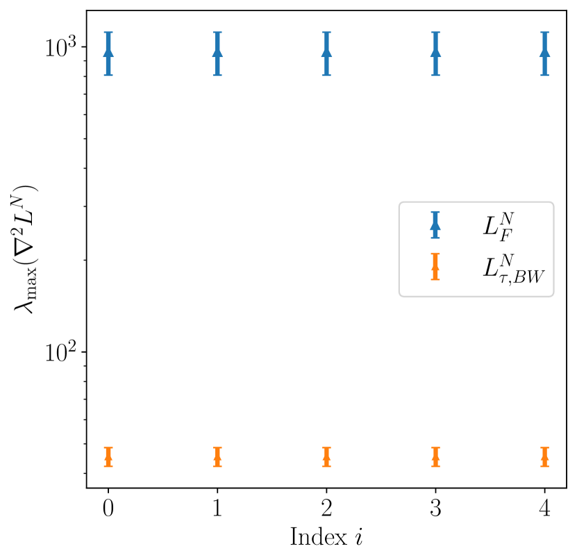
(a) Upper-bounds of the spectrum of $\nabla^{2}L^{N}$. There is an order of magnitude between the two losses.

(b) $\kappa_{\mathrm{rel}}(\nabla^{2}L^{N})$, in absolute value. Lower values are linked with better conditioned matrices.

(c) $\kappa_{\mathrm{abs}}(\nabla^{2}L^{N})$. Lower values are linked with better conditioned matrices.

Figure 2: Different spectral values for the Hessian matrices in the case $\tau=0.1$. The abscissa $i$ refers to the index of the critical point $W^{*}_{i}$. Mean and standard deviations are reported for seven different targets $\Sigma_{0}$.

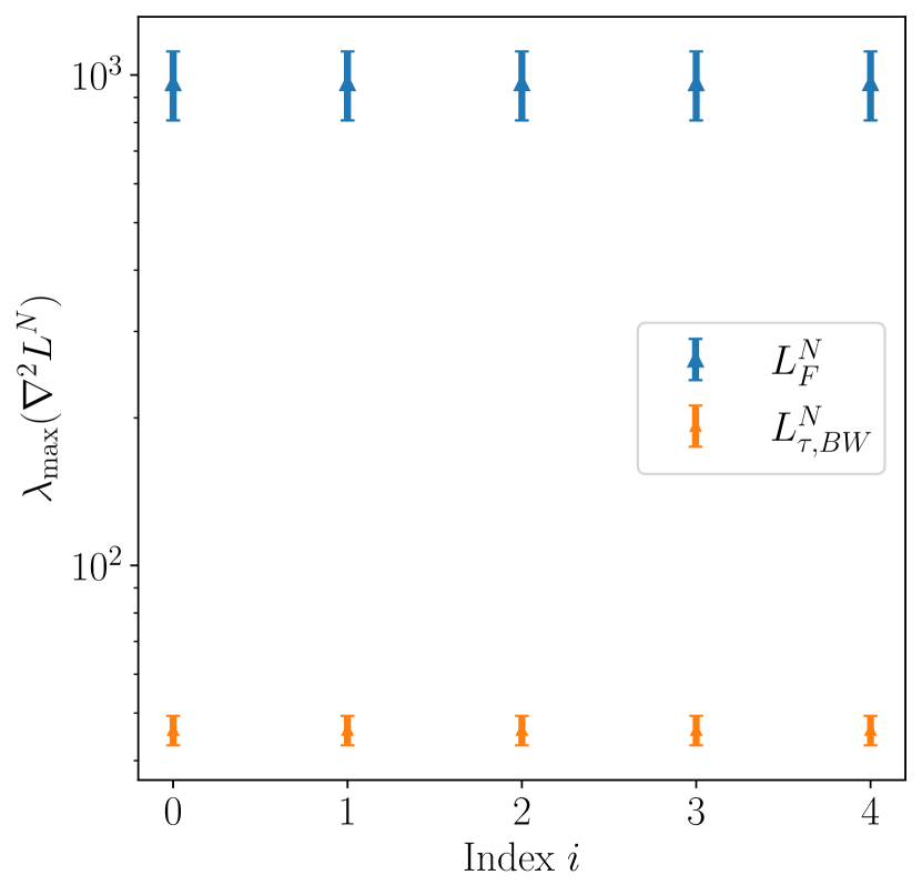
(d) Upper-bounds of the spectrum of $\nabla^{2}L^{N}$. There is an order of magnitude between the two losses.

(e) $\kappa_{\mathrm{rel}}(\nabla^{2}L^{N})$, in absolute value. Lower values are linked with better conditioned matrices.

(f) $\kappa_{\mathrm{abs}}(\nabla^{2}L^{N})$. Lower values are linked with better conditioned matrices.

Figure 3: Different spectral values for the Hessian matrices in the case $\tau=0.001$. The abscissa $i$ refers to the index of the critical point $W^{*}_{i}$. Mean and standard deviations are reported for seven different targets $\Sigma_{0}$.

References

• Absil et al. (2005) Absil, P. A., Mahony, R., and Andrews, B. Convergence of the Iterates of Descent Methods for Analytic Cost Functions. SIAM Journal on Optimization, 16(2):531–547, 2005.
• Arjovsky et al. (2017) Arjovsky, M., Chintala, S., and Bottou, L. Wasserstein Generative Adversarial Networks. In Proceedings of the 34th International Conference on Machine Learning, pp.  214–223. PMLR, 2017.
• Arora et al. (2018) Arora, S., Cohen, N., and Hazan, E. On the Optimization of Deep Networks: Implicit Acceleration by Overparameterization. In Proceedings of the 35th International Conference on Machine Learning, pp.  244–253, 2018.
• Arora et al. (2019a) Arora, S., Cohen, N., Golowich, N., and Hu, W. A Convergence Analysis of Gradient Descent for Deep Linear Neural Networks. In International Conference on Learning Representations, 2019a.
• Arora et al. (2019b) Arora, S., Cohen, N., Hu, W., and Luo, Y. Implicit Regularization in Deep Matrix Factorization. In Advances in Neural Information Processing Systems, volume 32, 2019b.
• Bah et al. (2021) Bah, B., Rauhut, H., Terstiege, U., and Westdickenberg, M. Learning deep linear neural networks: Riemannian gradient flows and convergence to global minimizers. Information and Inference: A Journal of the IMA, 11(1):307–353, 2021.
• Baldi & Hornik (1989) Baldi, P. and Hornik, K. Neural networks and principal component analysis: Learning from examples without local minima. Neural Networks, 2(1):53–58, 1989.
• Bhatia et al. (2019) Bhatia, R., Jain, T., and Lim, Y. On the Bures–Wasserstein distance between positive definite matrices. Expositiones Mathematicae, 37(2):165–191, 2019.
• Boumal (2022) Boumal, N. An introduction to optimization on smooth manifolds. To appear with Cambridge University Press, 2022. URL http://www.nicolasboumal.net/book.
• Bures (1969) Bures, D. An extension of Kakutani’s theorem on infinite product measures to the tensor product of semifinite $w$*-algebras. Transactions of the American Mathematical Society, 135:199–212, 1969.
• Chewi et al. (2020) Chewi, S., Maunu, T., Rigollet, P., and Stromme, A. Gradient descent algorithms for Bures-Wasserstein barycenters. In Conference on Learning Theory, pp.  1276–1304, 2020.
• Chitour et al. (2022) Chitour, Y., Liao, Z., and Couillet, R. A Geometric Approach of Gradient Descent Algorithms in Linear Neural Networks. Mathematical Control and Related Fields, 2022.
• Chulhee et al. (2018) Chulhee, Y., Suvrit, S., and Ali, J. Global optimality conditions for deep neural networks. In International Conference on Learning Representations, 2018. URL https://openreview.net/forum?id=BJk7Gf-CZ.
• De Meulemeester et al. (2021) De Meulemeester, H., Schreurs, J., Fanuel, M., De Moor, B., and Suykens, J. A. The bures metric for generative adversarial networks. In Machine Learning and Knowledge Discovery in Databases. Research Track: European Conference, ECML PKDD 2021, Bilbao, Spain, September 13–17, 2021, Proceedings, Part II 21, pp.  52–66. Springer, 2021.
• Dowson & Landau (1982) Dowson, D. C. and Landau, B. V. The Fréchet distance between multivariate normal distributions. Journal of Multivariate Analysis, 12(3):450–455, 1982.
• Dryden et al. (2009) Dryden, I. L., Koloydenko, A., and Zhou, D. Non-Euclidean statistics for covariance matrices with applications to diffusion tensor imaging. The Annals of Applied Statistics, 3(3):1102–1123, 2009.
• Du et al. (2018) Du, S. S., Hu, W., and Lee, J. D. Algorithmic Regularization in Learning Deep Homogeneous Models: Layers are Automatically Balanced. In Advances in Neural Information Processing Systems, volume 31, 2018.
• Dutta & Li (2017) Dutta, A. and Li, X. On a problem of weighted low-rank approximation of matrices. SIAM Journal on Matrix Analysis and Applications, 38(2):530–553, 2017.
• Eckart & Young (1936) Eckart, C. and Young, G. The approximation of one matrix by another of lower rank. Psychometrika, 1(3):211–218, 1936.
• Feizi et al. (2020) Feizi, S., Farnia, F., Ginart, T., and Tse, D. Understanding GANs in the LQG setting: Formulation, generalization and stability. IEEE Journal on Selected Areas in Information Theory, 1(1):304–311, 2020.
• Fukumizu (1998) Fukumizu, K. Effect of batch learning in multilayer neural networks. In In Proceedings of ICONIP’98, 1998.
• Gidel et al. (2019) Gidel, G., Bach, F., and Lacoste-Julien, S. Implicit regularization of discrete gradient dynamics in linear neural networks. In Advances in Neural Information Processing Systems, 2019.
• Gillis & Shitov (2019) Gillis, N. and Shitov, Y. Low-rank matrix approximation in the infinity norm. Linear Algebra and its Applications, 581:367–382, 2019.
• Gillis & Vavasis (2018) Gillis, N. and Vavasis, S. A. On the Complexity of Robust PCA and $\ell$1-Norm Low-Rank Matrix Approximation. Mathematics of Operations Research, 43(4):1072–1084, 2018.
• Hardt & Ma (2017) Hardt, M. and Ma, T. Identity matters in deep learning. In International Conference on Learning Representations, 2017. URL https://openreview.net/forum?id=ryxB0Rtxx.
• Helmke & Shayman (1995) Helmke, U. and Shayman, M. A. Critical points of matrix least squares distance functions. Linear Algebra and its Applications, 1995.
• Kantorovitch (1958) Kantorovitch, L. On the translocation of masses. Management Science, 5(1):1–4, 1958. URL http://www.jstor.org/stable/2626967.
• Kawaguchi (2016) Kawaguchi, K. Deep learning without poor local minima. In Advances in Neural Information Processing Systems, volume 29. Curran Associates, Inc., 2016. URL https://proceedings.neurips.cc/paper/2016/file/f2fc990265c712c49d51a18a32b39f0c-Paper.pdf.
• Kohn et al. (2022) Kohn, K., Merkh, T., Montúfar, G., and Trager, M. Geometry of linear convolutional networks. SIAM Journal on Applied Algebra and Geometry, 6(3):368–406, 2022. URL https://doi.org/10.1137/21M1441183.
• Kohn et al. (2023) Kohn, K., Montúfar, G., Shahverdi, V., and Trager, M. Function space and critical points of linear convolutional networks, 2023.
• Kroshnin et al. (2021) Kroshnin, A., Spokoiny, V., and Suvorikova, A. Statistical Inference for Bures–Wasserstein Barycenters. The Annals of Applied Probability, 31(3), 2021.
• Laurent & Brecht (2018) Laurent, T. and Brecht, J. Deep Linear Networks with Arbitrary Loss: All Local Minima Are Global. In Proceedings of the 35th International Conference on Machine Learning, pp.  2902–2907. PMLR, 2018. URL https://proceedings.mlr.press/v80/laurent18a.html.
• Liu et al. (2022) Liu, C., Zhu, L., and Belkin, M. Loss landscapes and optimization in over-parameterized non-linear systems and neural networks. Applied and Computational Harmonic Analysis, 59:85–116, 2022.
• Lu & Kawaguchi (2017) Lu, H. and Kawaguchi, K. Depth Creates No Bad Local Minima. arXiv.1702.08580, 2017.
• Magnus & Neudecker (2019) Magnus, J. R. and Neudecker, H. Matrix Differential Calculus with Applications in Statistics and Econometrics. Wiley Series in Probability and Statistics. Wiley, third edition edition, 2019.
• Mallasto et al. (2022) Mallasto, A., Gerolin, A., and Minh, Q. Entropy-regularized 2-Wasserstein distance between Gaussian measures. Information Geometry, 5(1):289–323, 2022.
• Masarotto et al. (2019) Masarotto, V., Panaretos, V., and Zemel, Y. Procrustes metrics on Covariance operators and optimal transportation of Gaussian processes. Sankhya A, 81(1):172–213, 2019.
• Mei et al. (2018) Mei, S., Montanari, A., and Nguyen, P. A mean field view of the landscape of two-layer neural networks. Proceedings of the National Academy of Sciences, 115(33):E7665–E7671, 2018.
• Min et al. (2021) Min, H., Tarmoun, S., Vidal, R., and Mallada, E. On the explicit role of initialization on the convergence and implicit bias of overparametrized linear networks. In Proceedings of the 38th International Conference on Machine Learning, pp.  7760–7768, 2021.
• Mirsky (1960) Mirsky, L. Symmetric Gauge Functions and Unitary Invariant Norms. The Quarterly Journal of Mathematics, 11(1):50–59, 1960.
• Muzellec & Cuturi (2018) Muzellec, B. and Cuturi, M. Generalizing Point Embeddings using the Wasserstein Space of Elliptical Distributions. In Advances in Neural Information Processing Systems, 2018.
• Nguegnang et al. (2021) Nguegnang, G. M., Rauhut, H., and Terstiege, U. Convergence of gradient descent for learning linear neural networks, 2021. URL https://arxiv.org/abs/2108.02040.
• Pele & Werman (2009) Pele, O. and Werman, M. Fast and robust earth mover’s distances. In 2009 IEEE 12th International Conference on Computer Vision, pp.  460–467, 2009.
• Ruben & Zamir (1979) Ruben, G. and Zamir, S. Lower rank approximation of matrices by least squares with any choice of weights. Technometrics, 21(4):489–498, 1979. URL http://www.jstor.org/stable/1268288.
• Saxe et al. (2014) Saxe, A. M., McClelland, J. L., and Ganguli, S. Exact solutions to the nonlinear dynamics of learning in deep linear neural networks. In 2nd International Conference on Learning Representations, ICLR 2014, Banff, AB, Canada, April 14-16, 2014, Conference Track Proceedings, 2014. URL http://arxiv.org/abs/1312.6120.
• Schmitt (1992) Schmitt, B. A. Perturbation bounds for matrix square roots and pythagorean sums. Linear Algebra and its Applications, 1992.
• Song et al. (2017) Song, Z., Woodruff, D. P., and Zhong, P. Low Rank Approximation with Entrywise L1-Norm Error. In Proceedings of the 49th Annual ACM SIGACT Symposium on Theory of Computing, STOC 2017, pp.  688–701, New York, NY, USA, 2017. Association for Computing Machinery.
• Tarmoun et al. (2021) Tarmoun, S., Franca, G., Haeffele, B. D., and Vidal, R. Understanding the Dynamics of Gradient Flow in Overparameterized Linear models. In Proceedings of the 38th International Conference on Machine Learning, pp.  10153–10161. PMLR, 2021. URL https://proceedings.mlr.press/v139/tarmoun21a.html.
• Trager et al. (2020) Trager, M., Kohn, K., and Bruna, J. Pure and spurious critical points: a geometric study of linear networks. In International Conference on Learning Representations, 2020. URL https://openreview.net/forum?id=rkgOlCVYvB.
• Villani (2003) Villani, C. Topics in Optimal Transportation. Graduate studies in mathematics. American Mathematical Society, 2003. URL https://books.google.com/books?id=idyFAwAAQBAJ.
• Villani (2008) Villani, C. Optimal Transport: Old and New. Grundlehren der mathematischen Wissenschaften. Springer Berlin Heidelberg, 2008. URL https://books.google.com/books?id=hV8o5R7_5tkC.
• Yun et al. (2021) Yun, C., Krishnan, S., and Mobahi, H. A unifying view on implicit bias in training linear neural networks. In International Conference on Learning Representations, 2021. URL https://openreview.net/forum?id=ZsZM-4iMQkH.