LABEL:fig:_GS2-evolutionshowsthetemporalevolutionofv(x, y, t)forahighresolutionAMRsimulationwithabaseresolutionof256^2cells.Thefivelevelsofrefinementallowforamaximaleffectiveresolutionof4096^2cells.Thislong-term,high-resolutionrunthenshowshowtheAMRquicklyadjuststotheself-replicating,morevolume-fillingpatternthatforms:whileatt=100thecoarsestgridoccupiesalargefractionof0.859ofthetotalarea,whilethefinestlevelcoversonlythecentral0.066area,thisevolvesto0.031(level1)and0.269(level5)attimet=3500,thelasttimeshowninFig.LABEL:fig:_GS2-evolution.Notethatonamodern20-CPUdesktop[usingIntelXeonSilver4210CPUat2.20GHz],thisentireruntakesonly1053seconds,ofwhichlessthan10percentisspentongenerating36completefiledumpsinboththenative.datformat,andtheon-the-flyconverted.vtuformat(suitableforvisualizationpackagessuchasParaVieworVisIt,seeSectionLABEL:sec:vtu).

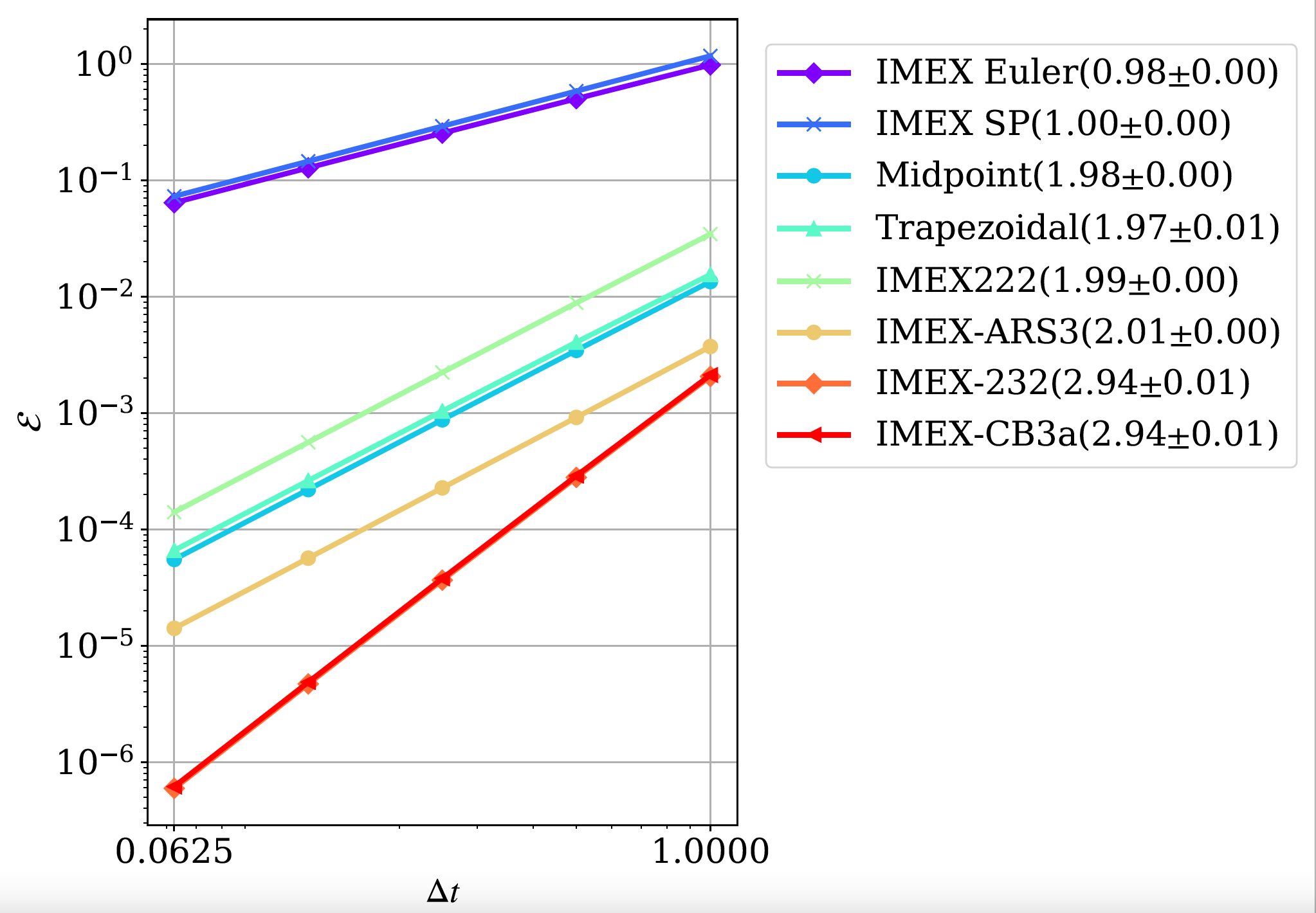
Figure 12: TemporalconvergenceofIMEX-RKschemesinMPI-AMRVAC.Theerrorcomputedas[∑_i=1^N(u[i]-u_ref[i])^2 + (v[i]-v_ref[i])^2]^1/2,whereNisthetotalnumberofgridpoints,isplottedasafunctionofthetimestepusedtoobtainthenumericalsolutionsuandvusingIMEXschemes.u_refandv_refarethereferencenumericalsolutionsobtainedusinganexplicitschemewithamuchsmallertimestep.

LABEL:fig:_GS2-evolution,butforauniformgridof256^2cells(correspondingtoacellsizeof≈0.01^2)andafinaltimet_end = 100(correspondingtothesecondpanelofFig.LABEL:fig:_GS2-evolution).Wecompareeverysimulationtoareferencesolutionobtainedwithaclassicalfourth-orderexplicitRunge-KuttaschemeforΔt = 10^-3.Whenexplicitlysolvingthereaction-diffusionsystemcorrespondingtotheinitialconditions,theexplicittimestepsareΔt_d, expl = 0.149andΔt_r, expl = 5.803associatedwithdiffusionandthereactionterms,respectively.Hence,theuseoftheIMEXschemesreducesthecomputationalcostbyafactorofΔt_r, expl/Δt_d, expl ≈39forthisparticularproblem.Fortheconvergenceteststhemselvesthevalueofthelargesttimestepisfixedtounity,followedbyfoursuccessivetimestepssmallerbyafactortwo.TheresultingconvergencegraphforΔt ∈{0.0625, 0.125, 0.25, 0.5, 1}isshowninFig.12,showinggoodcorrespondencebetweenthetheoreticalandobservedconvergencerates.

LABEL:eq:implicit)isactuallyaproblemthatcanberecasttothefollowingform

$$\nabla^{2}u^{a}-\frac{1}{\alpha\Delta tD_{u}}u^{a}=-\frac{1}{\alpha\Delta tD_{u}}u^{b}\,,$$ (34)

andsimilarlyforv.ForsolvingsuchgenericellipticproblemsonourAMRgrid,weexploittheefficientalgebraicmultigridsolverasintroducedin

2019Teunissen.Thistestisavailableattests/demo/Gray_Scott_2D.

5 Special(solar)physicsmodules

Inrecentyears,

MPI-AMRVAChasbeenactivelyappliedtosolarphysics,where3DMHDsimulationsarestandard,althoughtheymaymeetveryparticularchallenges.Evenwhenrestrictingattentiontothesolaratmosphere(photospheretocorona),handlingtheextremevariationsinthermodynamicquantities(density,pressureandtemperature)incombinationwithstrongmagneticfieldconcentrations,alreadyimplieslargedifferencesinplasmabeta.Moreover,aproperhandlingofthechromosphericlayers,alongwiththerapidtemperatureriseinanarrowtransitionregion,reallyforcesonetouseadvancedradiative-MHDtreatments(accountingforfrequency-dependent,non-localcouplingsbetweenradiationandmatter,truenon-local-thermal-equilibriumphysicsaffectingspectrallineemission/absorption,…).Thusfar,alltheseaspectsareonlyhandledapproximately,withe.g.therecentlyaddedplasma-neutralsrc/twoflmodule(2022Braileanu)asanexamplewheretheintrinsicallyvaryingdegreeofionizationthroughouttheatmospherecanalreadybeincorporated.Todealwithlargevariationsinplasmabeta,weprovidedoptionstosplitoffatime-independent(notnecessarilypotential)magneticfieldB_0inuptoresistiveMHDsettings(2018Xia),meanwhilegeneralized(nitin)tosplitoffentire3Dmagnetostaticforce-balancedstates-∇p_0+ρ_0g+J_0×B_0=0.ForMHDandtwo-fluidmodules,weaddanoptiontosolveinternalenergyequationinsteadoftotalenergyequationtoavoidnegativepressurewhenplasmabetaisextremelysmall.

Aspecificdevelopmentrelatestonumericallyhandlingenergyandmassfluxesacrossthesharptransitionregionvariation,whichundertypicalsolarconditionsandtraditionalSpitzer-typethermalconductivitiescanneverberesolvedaccuratelyinmultidimensionalsettings.Suitablymodifyingthethermalconductionandradiativelossprescriptionscanpreservephysicallycorrecttotalradiativelossesandheatingaspects

(2020Johnston).ThisledtotheTransition-Region-Adaptive-ConductionorTRACapproaches(2020Johnston; 2021Iijima; 2021Johnston; 2021Zhou),withe.g.2021Zhouintroducingvariousflavorswherethefieldlinetracingfunctionality(fromSectionLABEL:sec:trace)wasusedtoextendtheoriginally1Dhydroincarnationstomulti-dimensionalMHDsettings.Meanwhile,trulylocalvariants(2021Iijima; 2021Johnston)emerged,andMPI-AMRVAC 3.0providesmultipleoptionscollectedinsrc/mhd/mod_trac.t.Inpractice,upto7variantsoftheTRACmethodcanbedistinguishedinhigherdimensional(¿1D)setups,includingtheuseofagloballyfixedcut-offtemperature,the(maskedandunmasked)multi-dimensionalTRACLandTRACBmethodsintroducedin2021Zhou,orthelocalfixaccordingto2021Iijima.

Variousmodulesareavailablewhichimplementfrequentlyrecurringingredientsinsolarapplications.Theseare,e.g.,aPotential-Field-Source-Surface(PFSS)solutionona3Dsphericalgridthatextrapolatesmagneticfieldsfromagivenbottommagnetogram(seesrc/physics/mod_pfss.tasevaluatedin

2014Porth),amethodtoextrapolateamagnetogramintoalinearforce-freefieldina3DCartesianbox(seesrc/physics/mod_lfff.t),oramodularimplementationofthefrequentlyemployed3DTitov-Démoulin(1999TD)analyticfluxropemodel(seesrc/physics/mod_tdfluxrope.t),orthefunctionalitytoperformnon-linearforce-freefieldextrapolationsfromvectormagnetograms(seesrc/physics/mod_magnetofriction.tasevaluatedin2016Guo2; 2016Guo1).

Inwhatfollows,wedemonstratemorerecentlyaddedsolar-relevantfunctionality,namelytheadditionofatime-dependentmagnetofrictionalmoduleinSection

5.1,thepossibilitytoinsertfluxropesusingtheregularizedBiot-Savartlaws(RBSL)from2018TitovinSection5.2,andthewaytosynthesize3DMHDdatatoactualEUVimagesinasimpleon-the-flyfashioninSection5.3.

5.1 Magneto-frictionalmodule

Themagneto-frictional(MF)methodiscloselyrelatedtotheMHDrelaxationprocess

(e.g., 1981Chodura).Itisproposedby1986Yangandconsidersboththemomentumequationandthemagneticinductionequation:

ρ(∂v∂t + v⋅∇v) = J×B- ∇p + ρg -νv, (35)

∂B∂t = ∇×(v×B) , (36)

whereρisthedensity,vthevelocity,J=∇×B/μ_0theelectriccurrentdensity,Bthemagneticfield,pthepressure,gthegravitationalfield,νthefrictioncoefficient,andμ_0thevacuumpermeability.Toconstructasteady-stateforce-freemagneticfieldconfiguration,theinertial,pressure-gradient,andgravitationalforcesareomittedinEq.(

35)andoneonlyusesthesimplifiedmomentumequationtogivetheMFvelocity:

v= 1ν J×B. (37)

Eqs.(

36)and(37)arethencombinedtogethertorelaxaninitiallyfinite-forcemagneticfieldtoaforce-freestatewhereJ×B=0withappropriateboundaryconditions.

TheMFmethodhasbeenadoptedtoderiveforce-freemagneticfieldsin3Ddomains

(e.g., 1996Roumeliotis; 2005Valori; 2016Guo2; 2016Guo1).Itiscommonlyregardedasaniterationprocesstorelaxaninitialmagneticfieldthatdoesnotneedtohaveanobviousphysicalmeaning.Forexample,iftheinitialstateisprovidedbyanextrapolatedpotentialfieldtogetherwithanobservedvectormagneticfieldatthebottomboundary,thehorizontalfieldcomponentscanjumpdiscontinuouslythereinitially,andlocallyareprobablynotinadivergence-freecondition.TheMFmethodcanstillrelaxthisunphysicalinitialstatetoanalmostforce-freeanddivergence-freestate(thedegreeofforce-freenessanditssolenoidalcharactercanbequantifiedduringtheiteratesandmonitored).Ontheotherhand,theMFmethodcouldalsobeusedtoactuallymimicatime-dependentprocess(e.g., 2008Yeates; 2012Cheung),althoughtherearecaveatsaboutusingtheMFmethodinthisway(2013Low).Theadvantageofsuchtime-dependentMFmethodisthatitconsumesmuchlesscomputationalresourcesthanafullMHDsimulationtocoveralong-termquasi-staticevolutionofnearlyforce-freemagneticfields.Thisallowsustosimulatetheglobalsolarcoronalmagneticfieldoveraverylongperiod,forinstance,severalmonthsorevenyears.

WeimplementedanewMFmodule(src/mf),paralleltotheexistingphysicsmoduleslikeMHD,in

MPI-AMRVAC.Thismodulecanbeusedin2Dand3D,andindifferentgeometries,fullycompatiblewith(possiblystretched)block-AMR.Wesetthefrictioncoefficientν=ν_0 B^2 ,whereν_0=10^-15scm^-2isthedefaultvalue.ThemagnitudeoftheMFvelocityissmoothlytruncatedtoanupperlimitv_max=30kms^-1bydefaulttoavoidextremelylargenumericalspeednearmagneticnullpoints(Pomoell2019).ν_0andv_maxareinputparametersmf_nuandmf_vmaxwithdimensions.WeallowasmoothdecayoftheMFvelocitytowardsthephysicalboundariestomatchline-tiedquasi-staticboundaries(2012Cheung).IncontrasttothepreviousMFmodule(stillavailableassrc/physics/mod_magnetofriction.t)usedin2016Guo1,thisnewMFmoduleinsrc/mfincludesthetime-dependentMFmethodandnowfullyutilizestheframeworkfordataI/Owithmanymoreoptionsofnumericalschemes.Especially,theconstrainedtransportscheme(Balsara1999),compatiblyimplementedwiththestaggeredAMRmesh(Olivares2019),tosolvetheinductionequation(36)isrecommendedwhenusingthisnewMFmodule.Thisthencanenforcethedivergenceofmagneticfieldtonearmachineprecisionzero.

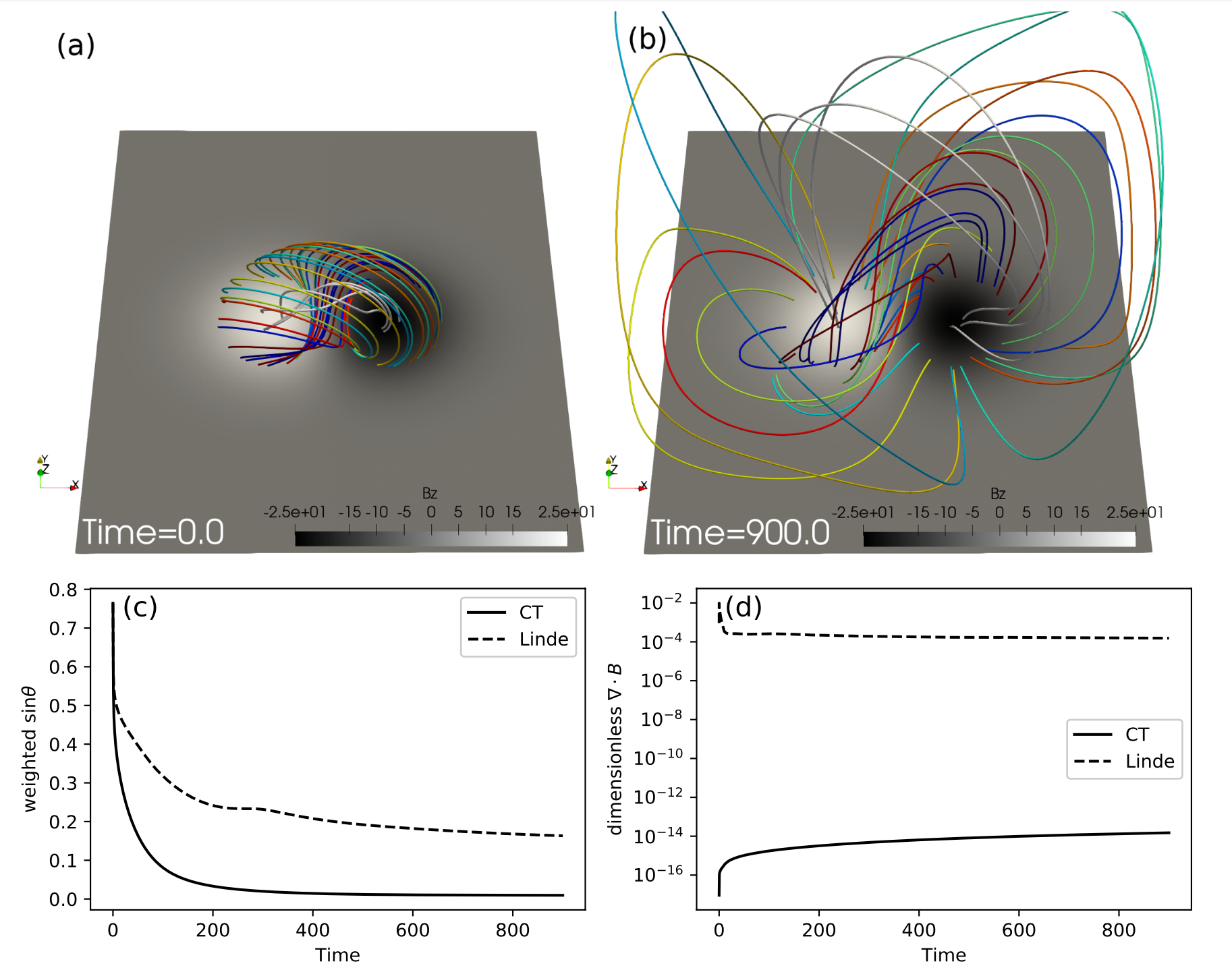
Figure 13: MFrelaxationofanon-force-freetwistedmagneticfluxtube.(a)magneticfieldlinesofthefluxtubeindifferentcolorsattime0,(b)magneticfieldlinesstartingfromthesamefootpointsattime900ofthe`ct′run,(c)degreeofforce-freeastheweightedaverageofthesineoftheanglebetweenthemagneticfieldandthecurrentdensityforthe`linde′and`ct′run,(d)degreeofdivergence-freeastheaveragedimensionlessdivergenceofthemagneticfieldforbothruns.

TovalidatethenewMFmodule,wesetupatest,fullyprovidedintests/demo/Mackay_bipole_Cartesian_3D,startingfromanon-force-freebipolartwistedmagneticfield

(Mackay2001)toverifythattheMFmodulecanefficientlyrelaxittoaforce-freestate.Themagneticfieldisgivenby

Bx=B0 e0.5(zL0e-ξ+4βxyL02e-2ξ) , (38)

By=2 βB0 e0.5(1-x2+z2L02)e-2ξ, (39)

Bz=B0 e0.5(-xL0e-ξ+4βyzL02e-2ξ) , (41)

ξ=0.5(x2+z2)+y2L02,

whereB_0=50Gisthepeakfluxdensity,β=1isadimensionlessparametertocontrolthetwistofthemagneticfield,andL_0=10Mmisthehalfdistancebetweenthepeaksoftwopolaritiesonthez=0boundary.Thetestisperformedina3DCartesianboxboundedby-40≤x≤40Mm,-40≤y ≤40Mm,and0≤z ≤80Mmwith4-levelAMRgridofeffective256×256×256resolution.The(magnetofrictional)velocitiesintheghostcellsaresettozero.Theinductionequationissolvedwithafinite-volumeschemecombiningtheHLLRiemannflux

(Harten83)withČada′sthird-orderlimiter(2009Cada)forreconstructionandathree-stepRunge--Kuttatimeintegration.Themagneticfieldisextrapolatedonthesideandtopboundariesassumingzeronormalgradient.Wecomparetwodivergencecontrolstrategies,namely`linde′versus`ct′(fromTableLABEL:t:divb).Intherunusing`linde′,weuseCourantnumber0.3forstabilityandadiffusivetermintheinductionequationdiminishesthedivergenceofthemagneticfield(Keppens03).Tokeepthebottommagneticfluxdistribution,themagneticfieldvectorsarefixedattheinitialvaluesinthefirst-layer(nexttothephysicaldomain)ghostcellsofthebottomboundaryandextrapolatedtodeeperlayersofghostcellswithdivergence-freecondition.Intherun`ct′,weuseCourantnumber0.8andtheconstrainedtransportmethodwiththeinitialface-centeredmagneticfieldintegratedfromtheedge-centeredvectorpotentialtostartwithzeronumericaldivergenceofthemagneticfield.Thetangentialelectricfieldonthebottomsurfaceisfixedtozerotopreservemagneticfluxdistribution.Magneticstructuresattheinitialtime0andthefinaltime900arepresentedbymagneticfieldlinesinFig.13aand13b,respectively.Theinitialtorus-likefluxtubeexpandsandrelaxestoatwistedfluxropewrappedbyshearedandpotentialarcades.InFig.13cand13d,wepresenttheforce-freedegreebytheweightedaverageofthesineoftheanglebetweenthemagneticfieldandthecurrentdensityasEq.(13)of2016Guo1andthedivergence-freedegreebytheaveragedimensionless∇⋅BastheEq.(11)of2016Guo1,respectively.Inthe`ct′run,theforce-freedegreerapidlydecreasesfrom0.76tolowerthan0.1withintime84,andconvergesto0.0095.Thedivergence-freedegreelevelsoffto1.5×10^-14.Intherunusing`linde′,theforce-freedegreedecreasessimilarlyuntil0.6andslowlyconvergestoaworsevalueof0.16.Thedivergence-freedegreequicklyreachesapeakvalueof0.098anddecreasesto1.5×10^-4.Furtherinvestigationlocatesthelarge∇⋅Berrorsatthetwomainpolaritiesinthefirst-layercellsabovethebottomboundaryinthe`linde′run.

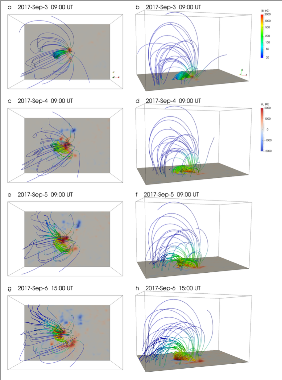
Figure 14: Evolutionofmagneticfieldlinesinthedata-driventime-dependentmagneto-frictionalsimulation.Theleftcolumnshowsatopviewandtherightcolumnshowsasideview.Thesliceonthebottomdisplaysnormalmagneticfield,B_z.Themagneticfieldlinesarecoloredbythefieldstrength.

WealsoapplythenewMFmoduletoobservations(providedintests/mf/data_driven_tmf)fortime-dependentevolution.Fig.

14showsanexampleoftheapplicationoftheMFmoduleinthesolaractiveregion12673.Weselectthetimerangebetween09:00UTon2017September3and15:00UTon2017September6todothesimulation,whichincludesthebuildupperiodfortwoX-classflarespeakingat09:10UT(X2.2)and12:02UT(X9.3)on2017September6,respectively.SDO/HMIobservesatemporalsequenceofvectormagneticfieldonthephotosphere.WeusetheSDO/HMIActiveRegionPatch(SHARP)datawithacadenceof12minutes(2014Hoeksema).Theseriesnameofthedatais``hmi.sharp_cea_720s.7115′′.ThevectorvelocityfieldisalsoderivedbytheinversionofthemagneticfieldusingtheDifferentialAffineVelocityEstimatorforVectorMagnetograms(DAVE4VM;2008Schuck).Then,boththetemporalsequenceofthevectormagneticfieldandthevelocityfieldareusedtofillthefirst-layerghostcellsatthebottomboundarytodrivetheevolutionofthecoronalmagneticfield.Theinitialconditionisapotentialfieldat09:00UTon2017September3asshowninFig.14a.Onauniform(domain-decomposed)gridof340×220×220cells,theinductionequationissolvedwiththesamenumericalschemesasinthe`linde′runofthebipolartest.ThemagneticfieldlineevolutioninFig.14indicatesthatatwistedmagneticfluxropeisformedalongthepolarityinversionlinetowardstheexplosionofthemajorflares.Theresulting3Dmagneticfieldevolutioncanbecomparedtoactualobservations(intermsoftheiremissionmorphology),orcanbeusedtostartfull3Dfollow-upMHDsimulationsthatincorporateactualplasmadynamics.

Notethatweheredidexploit`linde′divergencecontrol,sincethe`ct′methodrequiresastrictdivergence-freeboundaryconditionofmagneticfieldfornumericalstability.Forstaticcases(asinthemuchmoreidealizedtestfromFig.

13),thiscanberealizedeasily.However,fordatadrivenboundaryconditionsinwhichmagneticfieldsaredirectlygivenbyactualobservations,suchstrictdivergence-freeconditioncannotalwaysbeensured.Withthe`linde′method,spuriousdivergenceinducedbyadatadrivenboundarycanstillbediffusedandreduced,andthenumericalschemeisstableeventhoughlocallythediscretedivergenceofmagneticfieldcanberelativelylarge(asstatedaboveforthetestfromFig.13,typicallyinthefirstgridcelllayer).Whenwetriedtoapplythe`ct′methodtoactualSDOdata,codestabilitywascompromisedduetoresidualmagneticfielddivergence.Futureworkshouldfocusonmorerobust,fullyAMR-compatiblemeansforperformingdata-drivenrunsusingactualobservationalvectormagneticandflowdata.

5.2 InsertingfluxropesusingregularizedBiot--Savartlaws

Solareruptiveactivities,suchasflaresandCMEs,arebelievedtobedrivenbytheeruptionofmagneticfluxropes.Manyeffortshavebeendevotedtomodelthemagneticfieldofsuchaconfiguration,suchastheanalyticalGibson--Lowmodel

(1998Gibson),Titov--Démoulinmodel(1999Titov),andTitov--Démoulinmodifiedmodel(2014Titov).Alternatively,nonlinearforce-freefieldextrapolationsarealsoappliedtomodelfluxropesnumerically(e.g., 2009Canou; 2010Guo).Theyusethevectormagneticfieldobservedonthephotosphereastheboundarycondition,solvetheforce-freeequation∇×B= αB,andderivethe3Dcoronalmagneticfield.Therearesomedrawbacksintheseanalyticalandnumericalmethods.Mostanalyticalsolutionsassumesomegeometricsymmetries,suchasatoroidalarcintheTitov--Démoulinmodel.Ontheotherhand,manynumericaltechniquescannotderivefluxropestructuresinweakmagneticfieldregionorwhentheydetachfromthephotosphere,suchasforintermediateorquiescentprominences.Onewaytoalleviatethisproblemistoadoptthefluxropeinsertionmethod(2004vanBallegooijen).However,thismethodusesaninitialstatefarfromequilibrium,whichasksformanynumericaliterationstorelaxandthefinalconfigurationisdifficulttocontrol.

2018TitovproposedtheRBSLmethodtoovercometheaforementioneddrawbacks.Aforce-freemagneticfluxropewitharbitraryaxispathandintrinsicinternalequilibriumisembeddedintoapotentialfield.Theexternalequilibriumcouldbeachievedbyafurthernumericalrelaxation.TheRBSLmagneticfield,B_FR,generatedbyanetcurrentIandnetfluxFwithinathinmagneticfluxropewithaminorradiusa(l)isexpressedas:

BFR = ∇×AI + ∇×AF , (42)

AI(x) = μ0I4π∫C ∪C* KI(r) R’(l) dla(l) , (43)

AF(x) = F4π∫C ∪C* KF(r) R’(l) ×r dla(l)2 , (44)

whereA_I(x)andA_F(x)arethevectorpotentials,μ_0thevacuumpermeability,CandC^*theaxispathsaboveandbelowthereferenceplane,K_I(r)andK_F(r)theintegrationkernels,R’=dR/dltheunittangentialvector,lthearclengthalongtheaxispaths,andr ≡r(l) = (x - R(l))/a(l).

2018Titovhaveprovidedtheanalyticalformsoftheintegrationkernelsbyassumingastraightforce-freefluxropewithaconstantcircularcross-section.Theaxialelectriccurrentisdistributedinaparabolicprofilealongtheminorradiusofthefluxrope.Withsuchanalyticalintegrationkernels,afluxropewitharbitrarypathcouldbederivedviaEqs.(42)--(44).

2019Guo2implementedtheRBSLmethodinMPI-AMRVAC,nowavailableinthemodulesrc/physics/mod_rbsl.t.Themoduleworksfor3DCartesiansettings,allowingAMR.Fig.15showsthemagneticfluxropeconstructedbytheRBSLmethodoverlaidonthe304ÅimageobservedbySTEREO_B/EUVI.Inpractice,oneneedstodeterminefourparameterstocomputetheRBSLfluxrope,namely,theaxispathC,minorradiusa,magneticfluxF,andelectriccurrentdensityI.TheaxispathisdeterminedbytriangulationofstereoscopicobservationsofSTEREO_A/EUVI,SDO/AIA,andSTEREO_B/EUVIat304Å.Thesub-photosphericcounterpartC^*isthemirrorimageofCtokeepthenormalmagneticfieldoutsidethefluxropeunchanged.Theminorradiusisdeterminedbyhalfthewidthofthefilamentobservedin304Å.ThemagneticfluxisthendeterminedbythemagneticfieldobservedbySDO/HMIatthefootprintsofthefluxrope.Finally,theelectriccurrentI=(±52F)/(3μ_0 a),wherethesignisdeterminedbythehelicitysignofthefluxrope.

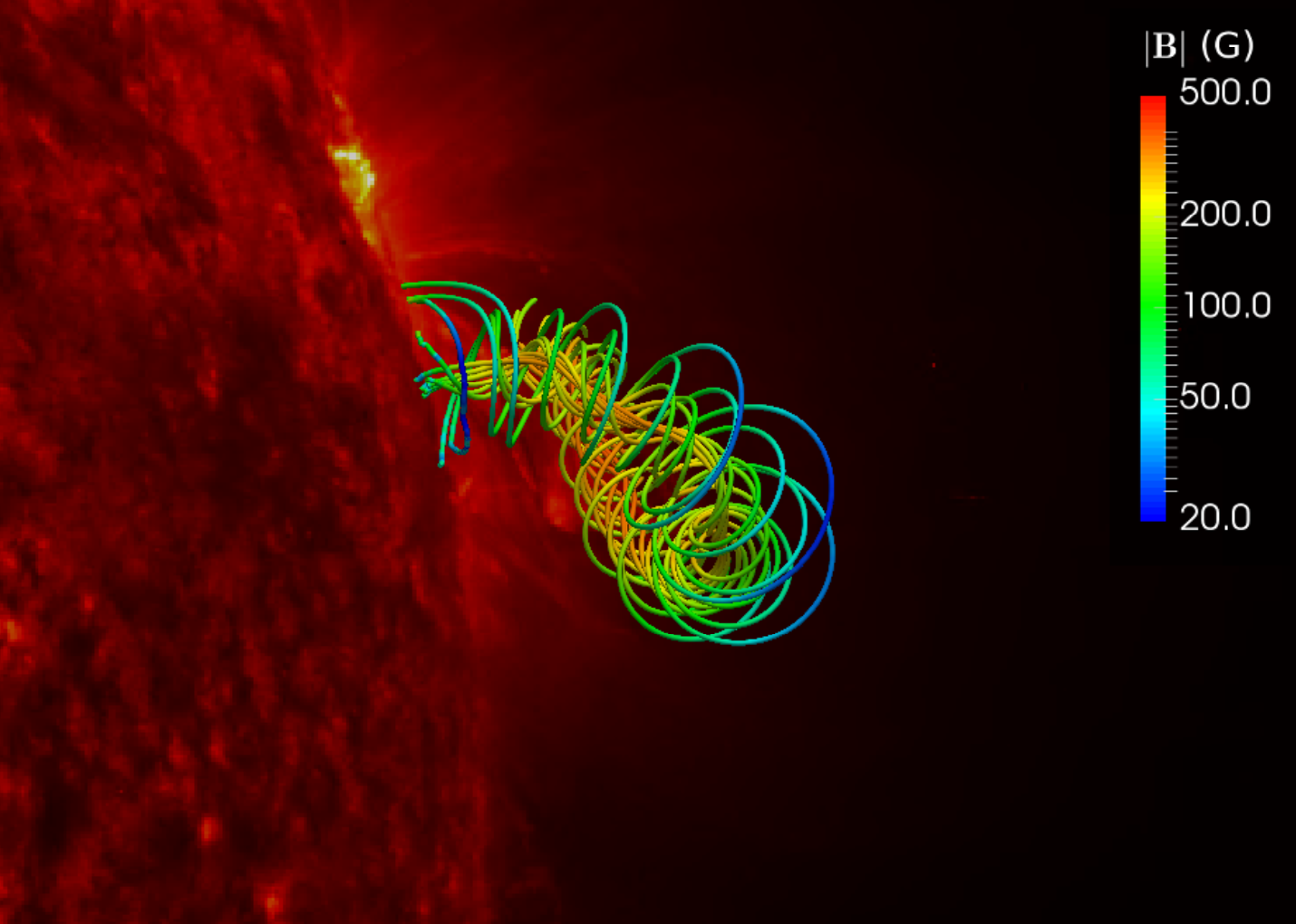
Figure 15: AmagneticfluxropeconstructedbytheregularizedBiot--Savartlaws(RBSL)overlaidontheSTEREO_B/EUVI304Åimageobservedat01:11UTon2011June11.

Withallthesefourparameters,theRBSLfluxropeiscomputedviaEqs.(

42)--(44).Ithastobeembeddedintoapotentialmagneticfieldtoconstructamagneticconfigurationconformingwithmagneticfieldobservations.WhenC^*isthemirrorimageofC,theRBSLfluxropehaszeronormalmagneticfieldoutsidethefluxrope,whilethemagneticfluxinsidethefluxropeisF.Therefore,wesubtractthemagneticfluxFinsidethetwofootprintstocomputethepotentialfield.TheRBSLfluxropefieldisembeddedintothispotentialfield.So,thenormalmagneticfieldonthewholebottomboundaryisleftunchanged.Thecombinedmagneticfieldmightbeoutofequilibrium.Wecouldrelaxthisconfigurationbythemagnetofrictionalmethod(2016Guo2; 2016Guo1).ThefinalrelaxedmagneticfieldisshowninFig.15.ThismagneticfieldcouldserveastheinitialconditionforfurtherMHDsimulations.

TheRBSLmethodcanalsobeappliedtoconstructtheanalyticalTitov--D

émoulinmodifiedmodel.Anexampleispresentedin2021Guo,wherethefluxropeaxishastobeasemicircularshape,anditisclosedbyamirrorsemicircleunderthephotosphere.ThemajorradiusR_cisafreeparameter.Thefluxropeaxisisplacedonthey=0planeanditscenterislocatedat(x,y)=(0,0).Theminorradiusaisalsoafreeparameter.Toguaranteetheinternalforce-freecondition,ahastobemuchsmallerthanR_c.Then,thefluxropehastobeembeddedintoapotentialfieldtoguaranteetheexternalforce-freecondition.Thepotentialfieldisconstructedbytwofictionalmagneticchargesofstrengthqatadepthofd_qunderthephotosphere,whicharealongthey-axisaty=±L_q.TheelectriccurrentandmagneticfluxaredeterminedbyEqs.(7)and(10)in2014Titov.

5.3 Syntheticobservations

Forsolarapplications,itiscustomarytoproducesyntheticviewson3Dsimulationdata,andvariouscommunitytoolshavebeendevelopedspecificallyforpost-processing3DMHDdatacubes.E.g.,theFoMocode

(2016Fomo)wasoriginallydesignedtoproduceopticallythincoronalEUVimagesbasedondensity,temperatureandvelocitydata,usingCHIANTI(see2021DelZannaandreferencestherein)toquantifyemissivities.FoMoincludesamorecompletecoverageofradioemissionofuptoopticallythickregimes,and2020PantprovidesarecentexampleofcombinedMPI-AMRVAC-FoMousageaddressingnon-thermallinewidthsrelatedtoMHDwaves.AnothertoolkitcalledFORWARD(2016Forward)includesthepossibilitytosynthesizecoronalmagnetometry,butisIdl-based(requiringsoftwarelicenses)andanimplementationforAMRgridstructuresisasyetlacking.

Sincesyntheticdataforespeciallyopticallythincoronalemissioniskeyforvalidationpurposes,wenowprovidemodulesthatdirectlyperformtheneededray-tracingonAMRdatacubes,insrc/physics/mod_thermal_emission.t.ThemodulecontainstemperaturetablesspecificforAIA,IRISandEISinstruments,withcoverageforvariouswavebands.OnecansynthesizebothEUVandsoftX-ray(SXR)emission,andthemodulecanbeusedforsyntheticimagesorforspectralquantifications.Imagesinvtiformatarereadilyproducedeitherduringruntime,orinapost-processingstep,wheretheusercontrolstherelativeorientationoftheline-of-sight(LOS)tothedatacube.Weusethisfor3DCartesiandatasetsfromMHD,allowingAMR.AsthefirststepinsynthesizinganEUVimage,a2Dtableiscreatedtorecordtheluminosityofeachimagepixel.WeassumethatanEUVimagehasuniformpixelsize,e.g.thepixelsizeofSDO/AIAimagesis0.6arcsec

(2012Lemen).ThespatiallinkbetweentheEUVimageplaneandthe3DsimulationboxreferstoFig.16a,wherethemappingbetweensimulationboxcoordinates(x,y,z)andEUVimagecoordinates(X,Y)isaccomplishedusingtheunitdirectionvectorsXIandYIoftheimageplaneatsimulationcoordinates:

(45)

(46)

ThevectorsXIandYIarebothperpendiculartothelineofsightandtoeachother,andaregivenby

XI = $$\@vec{V} \@vec{V}$$LOS×(0,0,1) —LOS×(0,0,1)— , (47)

YI = $$\@vec{X_{I}} \@vec{V} \@vec{X_{I}} \@vec{V}$$ ×LOS— ×LOS— , (48)

whereV_LOSisthelineofsightvectorinsimulationboxcoordinates.V_LOScanbewrittenas

$$\@vec{V}_{LOS}=(-\cos\varphi\sin\theta,-\sin\varphi\sin\theta,-\cos\theta),$$ (49)

withtheuser-givenparametersθandφ(Fig.

16b).Theuser-definedparameter(x_0,y_0,z_0),whichhasadefaultvalueof(0,0,0),canbeanypointinthesimulationboxandcanthenbemappedtotheEUVimagecoordinateorigin(X=0,Y=0).

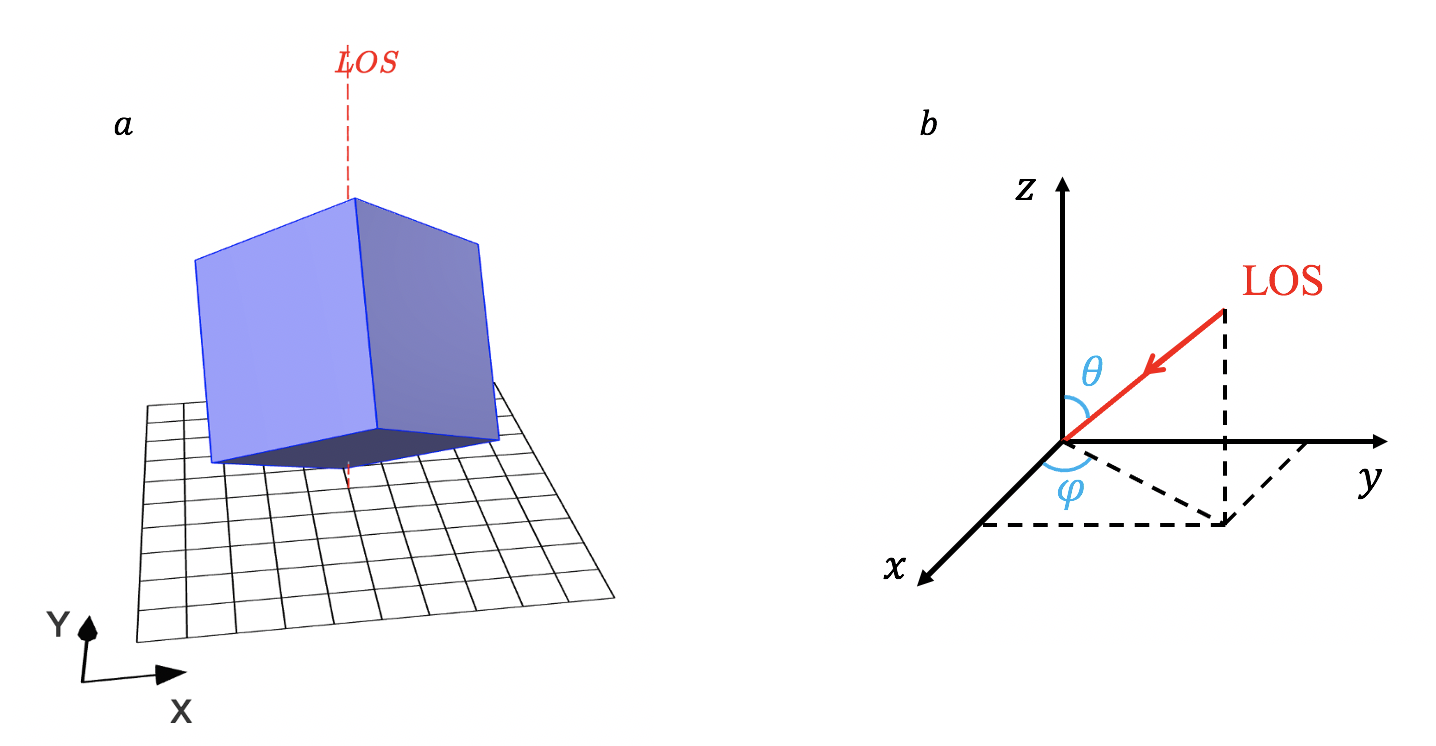
Figure 16: (a)Simulationbox(bluecube),LOS(reddashedline)andEUVimageplane(blackmesh).TheEUVimageplaneisperpendiculartoLOS.(b)LOSdependsonθandφatsimulationboxcoordinates.

TheintegralEUVfluxfromeachcellinthesimulationboxiscomputedandthendistributedoverthetable,wherethecellfluxisgivenby

$$I_{c}=N_{ec}^{2}G(T_{ec})\Delta x\Delta y\Delta z,$$ (50)

whereN_ecisthecellelectronnumberdensity,T_ecisthecellelectrontemperature,GisthecontributionfunctionofthecorrespondingEUVlinegivenbytheCHIANTIatomicdatabase,andΔx,Δy,andΔzarethecellsizesinthreedirections

(2021DelZanna).Duetoinstrumentscattering,asinglepointsourcewillappearasablobinEUVobservations.ThiseffectistakenintoconsiderationwhendistributingcellfluxtoimagepixelsbymultiplyingaGaussian-typepointspreadfunction(PSF)(2013Grigis).Theresultingpixelfluxisgivenby

Ip = ∑i Ic,i ∫XminXmax ∫YminYmax 12πσ2 (52)

×exp[-(X-Xc,i)2- (Y-Yc,i)22 σ2] dX dY

= ∑i Ic,i4 [erfc(Xmin-Xc,i2σ) - erfc(Xmax-Xc,i2σ)]

×[erfc(Ymin-Yc,i2σ) - erfc(Ymax-Yc,i2σ)],

whereiisthecellindex,I_c,iistheintegralEUVfluxfromtheithcell,(X_c,i,Y_c,i)isthemappingresultofthecellcenterattheimageplane,andX_min,X_max,Y_minandY_maxgivethebordersofthepixel.ThestandarddeviationσofthePSFistakenfromtherelatedpapersofthecorrespondingspacecraft,andisusuallyclosetothepixelsize.WhenthecellsizeisnotsmallenoughcomparedtotheEUVimagepixelsize(forexample,theprojectionofanycelledgeattheimageplaneislargerthanhalfthepixelsize),acellissplitintomultiplepartsbeforethecalculationofEqs.(

50)--(52)inordertoimprovetheintegralaccuracy.

Figure 17: Adata-drivenMHDmodel,withallenergeticsincorporated.Theverticalslicesshowthetemperatureontheleftanddensityontheright,respectively.Themagneticfieldlinesarecoloredbythefieldstrength.Thebottomslicedisplaysthenormalmagneticfield,B_z.

Fig.

17showsasnapshotofadata-drivenMHDmodelfortheX1.0flareat15:35UTon2021October28.The3DMHDmodelconsidersafullenergyequationwithbackgroundheating,thermalconduction,andopticallythinradiationlosses.Adetailedanalysisofthissimulationwillbepresentedinafuturepaper.Here,weuseasinglesnapshotfromtheevolutiontosynthesizeEUVimages,todemonstratethisnewcapabilityofMPI-AMRVAC.Fig.18showscomparisonsofSDO/AIAobservationsandthesynthesizedEUVimagesfromthedata-drivenMHDmodel.Weselectthreedifferentwavebandsat94Å,171Å,and304Å.ItisfoundthatthesimulationanditssynthesizedEUVimagesreproducesqualitativelyvariousaspectsseenintheflareribbons.Incontrasttotheactualobservedimages,coronalloopsarenotreproducedveryaccurately(asshowninFig.18cand18d),andthesimulationdisplaysarelativelystrongsphericalshockfront,seeninallthreewavebands.Theseaspectsrathercallforfurtherimprovementofthe(nowapproximate)radiativeaspectsincorporatedinthedata-drivenMHDmodel,butthesecanstillbeimprovedbyadjustingtheheating-coolingprescriptionsandthemagneticfieldstrength.Here,weonlyintendtoshowthesynthesizingabilityofMPI-AMRVAC,whichhasbeenclearlydemonstrated.

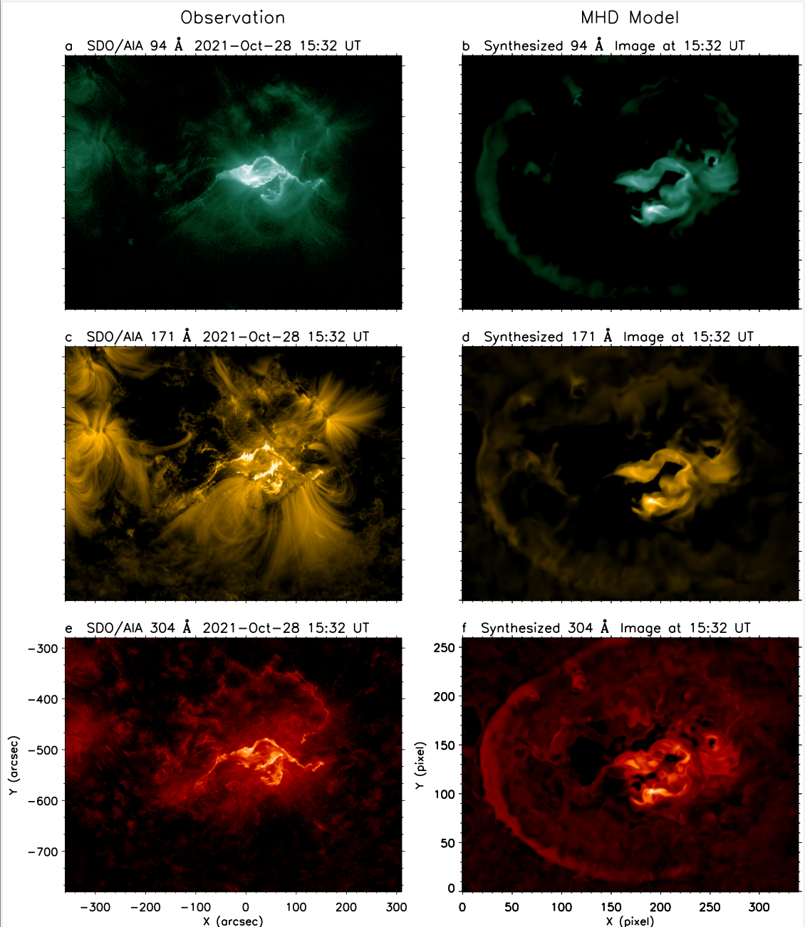
Figure 18: ComparisonbetweenSDO/AIAobservationsandsynthesizedEUVimagesfromadata-drivenMHDmodel(asinFig.17),includingafullenergytreatment.TheleftcolumnshowstheSDO/AIAobservationsatwavebandsof(a)94Å,(c)171Å,and(e)304Å.TherightcolumnshowstheemissionatthesamewavebandastheleftsynthesizedfromtheMHDmodelatthesametime.