Flexible and Efficient Simulation of Spatio-Temporal Processes with Advection

Abstract

Traveling phenomena are prevalent in a variety of fields, from atmospheric science to seismography and oceanography. However, there are two main shortcomings in the current literature: the lack of realistic modeling tools and the prohibitive computational costs for grid resolutions useful for data applications. We propose a flexible simulation method for traveling phenomena. To our knowledge, ours is the first method that is able to simulate extensions of the classical frozen field, which only involves one deterministic velocity, to a combination of velocities with random components, either in translation, rotation or both, as well as to velocity fields point-wise varying with space and time. We study extensions of the frozen field by relaxing constraints on its spectrum as well, giving rise to still stationary but more realistic traveling phenomena. Moreover, our proposed method is characterized by a lower computational complexity than the one required for circulant embedding, one of the most commonly employed simulation methods for Gaussian random fields, in $\mathbb{R}^{2+1}$.

Keywords: Traveling random field, simulation, computational efficiency, frozen field, velocity field, spectrum

AMS: 65D18, 42A16, 62P12

1 Introduction

Spatio-temporal processes are commonly observed in a number of application areas such as ocean and atmosphere science, environmetrics, epidemiology and geophysics. While there has been considerable advances in the simulation and estimation of the generating mechanism of stochastic processes in arbitrary spatial dimensions [19, 20, 22], the geometry of space-time is fundamentally different from 3-dimensional space. Some recent work, especially in modeling [36], have highlighted the differences between the geometry of 3-dimensional space and 2+1-dimensional space-time. The fundamental way 3-dimensional space and 2+1-dimensional space-time are different is that isotropy is a natural null model in the former scenario, but not at all in the latter scenario. A number of applied studies contain features that require new methodology, such as cyclones and more complex advection and transport [3, 21, 12, 32, 23, 6, 30]. These do require models able to capture more than a strict frozen field model.

What additional features then need to be incorporated into time-space modeling? We need to incorporate that what happens at one spatial point in time should be correlated with the same phenomenon that would have travelled to a new point at a later time. How does phenomena travel? The simplest understanding is to associate a velocity with any spatio-temporal point and assume it travels in time-space according to the specified velocity. This assumption is normally associated with the frozen field [36] if we only allow one velocity per field, and its extension for which the population of fields is associated with a set of random velocities, see e.g. [37], but we do not feel that this is sufficiently flexible to incorporate a bigger variety of patterns of behaviour. In addition, the previous literature does not address the problem of computationally efficient methods of simulation, a question we shall treat directly, especially important for traveling phenomena as the covariance function is not separable. There is a limit to how complex traveling phenomena can become as travel is characterised by a velocity, and this determines distance travelled unless the medium is compressible.

We shall start by understanding how it is possible to generalize the frozen field model, which relies on a deterministic constant velocity $\mathbf{v}$, to other more realistic, but still homogeneous phenomena. To do so, we study the frozen field spectrum, which concentrates the spatio-temporal process in frequency/wavenumber onto the lines of $\omega=-\mathbf{k}^{T}\mathbf{v}$, where $\omega$ is the temporal frequency and $\mathbf{k}$ is the spatial wavenumber. We start by replacing these lines of singularity with a more gentle decay, just like long-memory processes replace a seasonal harmonic process. Long-memory processes have been posited for random fields [26, 14], and can be relaxed into short-memory processes [17]. The former type of process has a set spectral decay, but are unbounded when $\omega=-\mathbf{k}^{T}\mathbf{v}$. Just like a long memory process can be regularized into a Matérn process, so has the author in [8, p. 396] suggested regularizing the covariance to elliptical contours, as well as more flexible alternatives.

We shall then consider even more general traveling phenomena, which we call heterogeneous traveling phenomena. Such phenomena include traveling fields whose velocities are either drawn from special orthogonal groups, allowing for both advection and rotation in complex ways, or defined point-wisely by a smooth velocity field. The latter is not stationary but generates realistically appearing spatio-temporal processes.

In summary, our developments correspond to a framework for understanding traveling phenomena, that is general, more realistic than any other framework presented in the past dedicated statistical literature and additionally can be simulated rapidly. The paper is organized as follows. We start by explaining how to model transport in Section 2, highlighting homogeneous processes in Section 2.1, and heterogeneous processes in Section 2.2. Section 3 highlights methods of simulations, and proceeds to illustrate features of the simulations via a number of concrete examples, as well as by discussing computational complexity of the proposed methods in Section 3.2. We conclude in Section 4. The supplementary materials provide further simulated examples, as well as the code to generate the plots presented.

2 Advection and Transport

What makes space-time processes fundamentally different from higher dimensional spatial processes is that phenomena travel in space with time, where traveling is associated with a particle moving on a trajectory with a local orientation in space and time. Isotropy assumes that the covariance behaves the same in all orientation, and is often no longer a reasonable assumption in this setting.

Let us start by introducing some notation. Let us assume that we study a continuous-space process $X_{S}({\mathbf{s}})$ taking values in ${\mathbb{R}}$ but where $\mathbf{s}\in{\mathbb{R}}^{d}$. We could study vector-valued processes ${\mathbf{X}}_{S}({\mathbf{s}})$ taking values in ${\mathbb{R}}^{p}$ but for simplicity we shall study scalar-valued processes. The authors of [36] have outlined the generalizations required when studying vector-valued processes for certain types of traveling phenomena. This would in general require more than one orientation, and is too complex a framework for our current setting. We shall instead focus on describing generalizations of univariate traveling phenomena by relaxing typical assumptions from the statistical literature regarding the velocity of any traveling component of the random fields.

In this document we shall assume that all processes are Gaussian. This assumption is commonly made, so that we can focus on the first two moments of the process, as these processes are then characterised by their first two moments

$${\mu} =\mathrm{E}\{X_{S}({\mathbf{s}})\}$$

$$c_{XX}(\mathbf{h}) =\mathrm{cov}\{X_{S}({\mathbf{s}}),X_{S}({\mathbf{s}+\mathbf{h}})\},$$

as we to start with additionally assume $X$ is spatially homogeneous (or stationary). Normally $\mu$ is referred to as the mean of the process, and $c_{XX}(\mathbf{h})$ as the auto-covariance sequence. Homogeneity is normally assumed if there is no reason to assume the process is inhomogeneous in space. Additionally some common assumptions on the auto-covariance sequence include symmetry, compact support and isotropy. An auto-covariance sequence is symmetric if $c_{XX}(\mathbf{h})=c_{XX}(-\mathbf{h}).$ The function $c_{XX}$ is said to be compactly-supported if it vanishes after a certain lag ${\mathbf{h}_{0}}$:

$$c_{XX}(\mathbf{h})=\begin{cases}c^{0}_{XX}(\mathbf{h}),&\text{if }||\mathbf{h}||\leq||\mathbf{h}_{0}||\\ 0&\text{otherwise}\end{cases}\,.$$ (1)

Finally $c_{XX}(\mathbf{h})$ is the covariance of an isotropic field if there is a function $c_{XX}^{(I)}(s)$ so that

$$c_{XX}(\mathbf{h})=c_{XX}^{(I)}(\|\mathbf{h}\|).$$ (2)

These assumptions are all realistic for spatial processes; but now we shall extend our modeling to spatio-temporal phenomena without assuming separability, namely that the temporal structure and the spatial structure can be studied separately. We start by discussing the simplest forms of non-separable spatio-temporal phenomena.

2.1 Homogeneous traveling Phenomena

The simplest example of a spatio-temporal phenomenon is variants of the traveling wave, namely the same temporal pattern that is shifted in space. We shall start with the plane wave, where a temporal phenomenon is replicated in space.

Definition 2.1 (Plane wave [8]).

A spatio-temporal structure $Z(\mathbf{s},t)$ is a plane wave, if there is a stationary time process in $\mathbb{R}$ $X_{T}(t)$, a direction $\bm{\eta}\in{\mathbb{R}}^{d}$ and a velocity $v\in{\mathbb{R}}$ such that

$$Z(\mathbf{s},t)=X_{T}\left(t-\frac{\bm{\eta}^{T}\mathbf{s}}{v}\right).$$ (3)

This phenomenon corresponds to a 1-dimensional temporal signal $X_{T}(t)$ getting shifted in time $t$ depending on its spatial location $\mathbf{s}$ (imagining that it takes time for the signal to travel in space). In general this is an overly simplistic view of spatio-temporal, and we will only show a simulated example in the supplementary materials.

How can we get inspired to model more complex phenomena from these basic components? A natural inspiration is spatio-temporal phenomena arising in hyperbolic partial differential equations, whose solutions take the form of $Z(\mathbf{s},t)=X_{S}(\mathbf{s}-\mathbf{v}t)$ ([15], [8]). We can then recall the definition of the stochastic process corresponding to this phenomenon.

Definition 2.2 (Frozen field [8]).

A random field $Z(\mathbf{s},t)$ is a frozen field if there is a constant velocity $\mathbf{v}\in{\mathbb{R}}^{d}$, and a random field $X_{S}(\mathbf{s})$ with $\mathbf{s}\in{\mathbb{R}}^{d}$ and covariance function $c_{XX}^{(S)}(\mathbf{h})$ such that

$$Z(\mathbf{s},t)=X_{S}(\mathbf{s}-\mathbf{v}t),$$ (4)

with $t\in\mathbb{R}^{+}$. We call $(\mathbf{v}\tau,\tau)$ the propagation path, as it determines the point where a location will be transported to at time point $\tau$ starting at the origin.

Unfortunately, while the frozen field can be more complex than the plane wave, it is still not a sufficiently flexible model to describe many realistic phenomena. Let us determine the covariance and the spectrum of the frozen field model before we construct more flexible models.

Proposition 2.1 (Second order structure of the frozen field).

Assume that the process $Z(\mathbf{s},t)$ is a frozen field. Then the covariance function and spectrum of $Z(\mathbf{s},t)$ take the form

$$c_{ZZ}(\mathbf{h},\tau) =c_{XX}^{(S)}(\mathbf{h}-\mathbf{v}\tau)$$ (5)

$$S_{ZZ}(\mathbf{k},\omega) =S_{XX}^{(S)}(\mathbf{k})\cdot\delta(\omega+\mathbf{k}^{T}\mathbf{v}).$$ (6)

What have then researchers done to relax this assumption so that more realistic phenomena can be modeled? Commonly a distribution is put on the true orientation, and a single vector is therefore drawn for the field from a chosen distribution [37]. However with this randomly selected orientation, it is still assumed from (4) that a perfect and deterministic relationship holds between the field at different point in time and space. This is too constrained for many realistic scenarios. The authors of [36] offered a generalization by defining a multivariate signal which is subject to multiple advections/orientations. We shall wish to be less constrained in our specification allowing for a distribution of velocities across the process.

The field also clearly satisfies Taylor’s hypothesis that

$$c_{ZZ}(\mathbf{v}\tau,0)=c_{XX}^{(S)}(\mathbf{v}\tau)=c_{ZZ}(\mathbf{0},\tau),$$ (7)

which is a common assumption in fluid mechanics, but causes perfect correlation while the observer stays inside the traveling wave of $\mathbf{h}-\mathbf{v}\tau$. However, normally we would not expect a phenomena to persist over all positive lag. We would instead expect a dissipation of energy over time [8]. This replaces a decay in $\|\mathbf{h}-\mathbf{v}\tau\|^{2}$ with a decay in $\|\mathbf{h}-\mathbf{v}\tau\|^{2}+(u\tau)^{2}$. The extra term causes an extra decay as the distance between two points in time increases. The additional term has precisely been added to ensure that as the lags get bigger, the correlation decays. We shall however start by proposing homogeneous fields with well-defined mean orientation that exhibit a range of orientations.

Our first proposal to generalize the frozen field is carried out by relaxing the assumptions regarding the shape of its spectrum. Most patterns from applications are not as exact as the simplest mathematical models would make them. Studying the proposed spectral nature of the frozen field, viz. (6), it would be more realistic to nearly have a weaker singularity at $\omega=-\mathbf{k}^{T}\mathbf{v}$. What is then a “weaker singularity”? It has to be integrable to produce a process that has finite variance. How do we then produce a weaker singularity? We take inspiration from seasonally persistent processes that are nearly but not quite cyclical [31]. This produces orientationally persistent frozen fields.

Definition 2.3 (Orientationally persistent frozen field).

We define the orientationally persistent frozen field as the zero-mean time-space Gaussian random process for persistence parameter $\delta\in(0,1/2)$ which has spectrum

$$S_{ZZ}(\mathbf{k},\omega)=S_{XX}^{(S)}(\mathbf{k})\cdot\|\omega+\mathbf{k}^{T}\mathbf{v}\|^{-2\delta},\quad\mathbf{k}\in(-\pi,\pi)^{2},\quad\omega\in(-\pi,\pi).$$ (8)

This process replaces the exact delta-function in (6) by a singularity, where $\delta$ governs the decay of the wave-like phenomenon.

Waves represent an exact relationship between space and time. This corresponds to a singularity in the frequency/wavenumber domain. To generate spatio-temporal phenomena that generates wave-like behaviour we replace the delta function by a weaker singularity. Weaker singularities in the frequency domain are used to generate self-similar processes such as fractional Brownian motion (fBm). We shall use this mechanism. We note that when specifying fBm some care must be used. It contains a powerlaw, which for the stochastic processs to be stationary must have finite variance. We take inspiration from long-correlation models, see [14], where the discrete sampling is acknowledged directly. In two dimensions we want to define a genuinely discrete process so we do not have to deal with aliasing. The continuous spatio-temporal process we would like to define is, starting from the special case of $S^{(S)}_{XX}(\mathbf{k})=S_{0}\in{\mathbb{R}}^{+}$,

$$c_{ZZ}(\mathbf{h},\tau) =S_{0}\iiint\|\omega+\mathbf{k}^{T}\mathbf{v}\|^{-2\delta}\,e^{2\pi i(\omega\tau+\mathbf{k}^{T}\mathbf{h})}\,d\omega\,d^{2}\mathbf{k}.$$ (9)

Does this specify a valid process? One check would be to retain the symmetry when $(\omega,\mathbf{k})$ maps to $(-\omega,-\mathbf{k})$. Secondly this is related to long-memory processes, and for random fields, there is a literature to refer to [14, 26, 2]. To get a genuine discrete process we have to be careful. Using the Cartesian differencing operators will not lead to an isotropic spectrum, and for $S_{XX}^{(S)}(\mathbf{k})$ to be isotropic we need to define a genuinely isotropic process, see work by [40, 24]. The term $\|\omega+\mathbf{k}^{T}\mathbf{v}\|^{-2\delta}$ ensures that $\mathbf{s}=t\mathbf{v}$ is not perfectly adhered to, and it is replaced by $\mathbf{s}\approx t\mathbf{v}.$ This does not need special discretization and corresponds to smoothing along the wave.

Most realistic processes exhibit dissipation. This is why the Matérn process, see for instance [39], is often more useful as a modeling tool for geophysical processes than say fBm [27]. The Matérn version of this spatio-temporal process would include damping. We therefore define the following process to accommodate such structure.

Definition 2.4 (Damped frozen field).

We define the damped frozen field as a zero-mean Gaussian stochastic process for persistence parameter $\delta\in(0,1/2)$ and damping parameter $h>0$ with spectrum:

$$S_{ZZ}(\mathbf{k},\omega)=S_{XX}^{(S)}(\mathbf{k})\cdot\|(\omega+\mathbf{k}^{T}\mathbf{v})^{2}+h^{2}\|^{-\delta},\quad\mathbf{k}\in(-\pi,\pi)^{2},\quad\omega\in(-\pi,\pi),\;h>0.$$ (10)

Why would we like to consider all these different processes for spatio-temporal phenomena? Just like for temporal processes, understanding processes with a certain large frequency spectral decay, versus boundedness at small frequencies, allows us to understand different types of phenomena, see for example examples such as cyclones and more complex advection and transport [3, 21, 12, 32, 23, 6, 30].

Now to realistically capture that phenomena that dissipate, the author of [9, p. 396] proposed covariance functions with elliptical contours. This would correspond to a damping that was frequency dependent. This leads to the following definition:

Definition 2.5 (Frequency-dependent damped frozen field).

We define the frequency-dependent damped frozen field as a zero-mean Gaussian stochastic process for persistence parameter $\delta\in(0,1/2)$ and damping parameter $a>0$ with spectrum:

$$S_{ZZ}(\mathbf{k},\omega)=S_{XX}^{(S)}(\mathbf{k})\cdot\|(\omega+\mathbf{k}^{T}\mathbf{v})^{2}+(a\omega)^{2}\|^{-\delta},\quad\mathbf{k}\in(-\pi,\pi)^{2},\quad\omega\in(-\pi,\pi).$$ (11)

This spectral density decays eliptically and is nicely bounded as long as we avoid $\omega=0$. Now these types of processes that we have defined are all homogeneous in time and space, but in general traveling phenomena are heterogeneous in time, space or space-time. Let us discuss what alternatives we may propose to capture such scenarios.

2.2 Heterogeneous traveling Phenomena

Imagine instead of observing the perfectly replicated traveling phenomenon the medium which the wave is traveling through is not perfectly homogeneous, and in a consistent fashion. The orientationally selective field fluctuates around a frozen field, but in a non-predictive manner. In real-life scenarios we might instead have a heterogeneous material that a particle is passing through. Thus the geometry of the traveling wave specified by (5) is too strict to describe the phenomenon we observe. How would then a phenomenon be visited across time and space? We need to observe the underlying $d$-dimensional phenomenon not at spatial location $\mathbf{s}-\mathbf{v}t$. Imagine that now $\mathbf{v}$ is changing in time and space. A particle in a phenomenon would then travel according to $\mathbf{v}(\mathbf{s},t)$. Where would then in general a particle travel to? Starting from position $\mathbf{s}$ and time 0, we expect the particle to end up at

$$\mathbf{s}+\int_{0}^{t}\int_{\mathbf{s}}\mathbf{v}(\mathbf{s}^{\prime},t^{\prime})\,d\mathbf{s}^{\prime}dt^{\prime}.$$

There are really no assumptions required for this expression to hold. We then need to model this lack of homogeneity. We shall explore some modeling options. The first choice we shall explore will assume heterogeneity of material the wave moved through but no patterned heterogeneity. We shall call this the distributed frozen field, as it is realized with a distribution of present velocities, that are not patterned but variable.

Definition 2.6 (Random velocity frozen field [11, 38] and [8], p. 396).

The spatial random field $X_{S}(\mathbf{s})$ is generated, then a random velocity (field) $\mathbf{v}$ is used to shift this field. After generating a large spatial process $X_{S}(\mathbf{s})$ the random velocity process is then defined according to

$$Z(\mathbf{s},t)=X_{S}(\mathbf{s}-\mathbf{v}(\mathbf{s},t)\cdot t),\quad\mathbf{v}(\mathbf{s},t)\sim{\cal N}(\bm{\mu},D),$$ (12)

where $\bm{\mu}$ is a $d\times 1$ vector and $D$ is a $d\times d$ covariance matrix.

We shall now understand this process: the spatial process $X_{S}(\mathbf{s})$ is shifted slightly differently at each space-time point by an iid random velocity (this is according to [8]), while [37] only generates a random orientation once for the whole field). This may not realistically reproduce all patterns we see. The first random velocity frozen field would be to take the same field and at random shift it slightly differently.

How much can we generalize the notion of frozen field? At the heart lies the notion of transport and advection. As long as we assume the medium is incompressible, this is governed by Newton’s laws of motion. How can we then further generalize the notion of a single traveling phenomenon? Can we use more than one velocity? Let us explore this further.

Definition 2.7 (Distributed frozen field).

A random field $Z(\mathbf{s},t)$ is a distributed frozen field if there is a set of velocities $\mathbf{v}_{i}\in SO(d)$, and a random field $X_{S}(\mathbf{s})$ with $\mathbf{s}\in{\mathbb{R}}^{d}$ and covariance function $c_{XX}^{(S)}(\mathbf{h})$ such that

$$Z(\mathbf{s},t)=\int_{SO(d)}p(\mathbf{v}_{\theta})X_{S}(\mathbf{s}-\mathbf{v}_{\theta}t)\,d\mathbf{v}_{\theta},$$ (13)

with $t\in\mathbb{R}^{+}$ and $SO(d)$ denoting the special orthogonal group [10], namely the group of all rotations about the origin of $d$-dimensional Euclidean space.

Depending on the form of $p(\mathbf{v}_{\theta})$ this will produce a more or less structured appearance of the spatio-temporal phenomenon. This specification of (13) can be discretized as

$$Z(\mathbf{s},t) =\sum_{i=1}^{n_{\text{v}}}p(\mathbf{v}_{i})X_{S}(\mathbf{s}-\mathbf{v}_{i}t),$$ (14)

using a set of possible velocities $\mathbf{v}_{1},\dots,\mathbf{v}_{n_{\text{v}}}$ with associated probabilities/weights $p(\mathbf{v}_{1}),\dots,p(\mathbf{v}_{n_{\text{v}}})$.

In some settings it is more natural to assume the random field locally satisfies the wave equation. This means for every spatial location $\mathbf{s}$ and time point $t$ we define a velocity field $\mathbf{v}(\mathbf{s},t)$ defining a velocity at that time and spatial point. Assuming $Z(\mathbf{s},t)$ locally satisfies the wave equation then we get the following stochastic process:

Definition 2.8 (Evolving frozen field).

A random field $Z(\mathbf{s},t)$ is a evolving frozen field if there is a deterministic velocity field $\mathbf{v}(\mathbf{s},t)\in{\mathbb{R}}^{d}$, and a random field $X_{S}(\mathbf{s})$ with $\mathbf{s}\in{\mathbb{R}}^{d}$ and covariance function $c_{XX}^{(S)}(\mathbf{h})$ such that

$$Z(\mathbf{s},t)=X_{S}(\mathbf{s}-\mathbf{v}(\mathbf{s},t)\cdot t),$$ (15)

with $t\in\mathbb{R}^{+}$.

We see a number of special cases here: one where the field is constant in time $t$ but varies in space, e.g. $\mathbf{v}(\mathbf{s},t)=\mathbf{v}(\mathbf{s})$, so-called steady flow, that is $\frac{\partial}{\partial t}\mathbf{v}(\mathbf{s},t)=\mathbf{0}$. Common examples of steady flow include stagnation points, $\mathbf{v}(\mathbf{s})=(ks_{1},\;-ks_{2})$ for $k>0,$ rigid body rotation $\mathbf{v}(\mathbf{s})=(-ks_{2},\;ks_{1})$, a vortex $\mathbf{v}(\mathbf{s})=(-ks_{2}/s,\;ks_{1}/s)$ for $s=\sqrt{s_{1}^{2}+s_{2}^{2}}$, and a source and a sink, $\mathbf{v}(\mathbf{s})=(ks_{1}/s,\;ks_{2}/s)$. Or we could also assume the velocity is constant in space, but instead varies in time, $\mathbf{v}(\mathbf{s},t)=\mathbf{v}(t)$. An additional potential is to assume that $\mathbf{v}(\mathbf{s},t)$ is incompressible flow e.g. $\nabla\cdot\mathbf{v}(\mathbf{s})=0$, or irrotational flow e.g. $\nabla\times\mathbf{v}(\mathbf{s})=\mathbf{0}$ (for a comprehensive insight see for instance [25]).

We shall determine the mathematical properties of the evolving frozen field, which is linked to an unobserved velocity field in Definition 2.8. Velocity fields are commonly studied in fluid mechanics, and here correspond to a latent infinite dimensional parameter. If we are trying to simulate processes, this field provides more realistic realized patterns. If we are trying to estimate it from data, then we are trying to recover the generating mechanism of the process, while using as few degrees of freedom in the process as possible. However, just like we can estimate non-parametric functions, we can seek to estimate the latent velocity field, depending on our form of observations, and other assumptions. By constructing a 3-dimensional process, from a 2-dimensional process coupled with a smooth deterministic function, we are making lower dimensional subspaces in nominally high dimensional data. The inference aim for such a setting, is what properties can be inferred from a single observed sampled random field.

The evolving frozen field is clearly an inhomogeneous process, but we can interpret the inhomogeneity, unlike for a distributed frozen field, where this latent pattern is random, and where every aspect of the realization might not be interpretable.

Proposition 2.2.

Assume that $Z(\mathbf{s},t)$ is an evolving frozen field as specified by Definition 2.8. The propagation path is then

$$\left((\mathbf{I}-D_{\mathbf{s}}(\mathbf{s},t)(t+\tau))^{-1}\left\{\mathbf{v}(\mathbf{s},t)+D_{t}(\mathbf{s},t)(t+\tau)\right\}\tau,\tau\right).$$ (16)

Proof.

To determine the propagation path we need to determine the covariance of the evolving frozen field. To arrive at an interpretable expression we apply local expansions on $\mathbf{v}(\mathbf{s},t)$. We express the velocity field locally to be:

$$\mathbf{v}(\mathbf{x}+\mathbf{h},t+\tau)=\mathbf{v}(\mathbf{x},t)+{\mathbf{D}}_{\mathbf{x}}(\mathbf{x},t)\mathbf{h}+D_{t}\tau+O(\|\mathbf{h}\|^{2})+O(\tau^{2}),$$ (17)

where ${\mathbf{D}}_{\mathbf{x}}(\mathbf{x},t)=\begin{pmatrix}\frac{\partial\text{v}_{1}(\mathbf{x},t)}{\partial x_{1}}&\frac{\partial\text{v}_{1}(\mathbf{x},t)}{\partial x_{2}}\\ \frac{\partial\text{v}_{2}(\mathbf{x},t)}{\partial x_{1}}&\frac{\partial\text{v}_{2}(\mathbf{x},t)}{\partial x_{2}}\end{pmatrix}$ and $D_{t}(\mathbf{x},t)=\left(\frac{\partial\text{v}_{1}(\mathbf{x},t)}{\partial t},\frac{\partial\text{v}_{2}(\mathbf{x},t)}{\partial t}\right)^{T}$. Hence, the covariance is

$$\mathrm{cov}\left\{X(\mathbf{x}-\mathbf{v}(\mathbf{x},t)t),X(\mathbf{x}+\mathbf{h}-\mathbf{v}(\mathbf{x}+\mathbf{h},t+\tau)(t+\tau))\right\}$$

$$=c_{XX}\left(\mathbf{h}-\left(\mathbf{v}(\mathbf{x}+\mathbf{h},t+\tau)(t+\tau)-\mathbf{v}(\mathbf{x},t)t\right)\right)$$

$$=c_{XX}\left(\mathbf{h}-\left\{\mathbf{v}(\mathbf{x},t)+{\mathbf{D}}_{\mathbf{x}}(\mathbf{x},t)\mathbf{h}+D_{t}(\mathbf{x},t)\tau+O(\|\mathbf{h}\|^{2})+O(\tau^{2})\right\}(t+\tau)+\mathbf{v}(\mathbf{x},t)t\right)$$

$$=c_{XX}\left(\mathbf{h}-\mathbf{v}(\mathbf{x},t)\tau-\left\{{\mathbf{D}}_{\mathbf{x}}(\mathbf{x},t)\mathbf{h}+D_{t}(\mathbf{x},t)\tau+O(\|\mathbf{h}\|^{2})+O(\tau^{2})\right\}(t+\tau)\right).$$ (18)

Unity correlation happens when the argument of (2.2) is zero. This corresponds to the spatial and temporal lags of

$$\mathbf{h}-\mathbf{v}(\mathbf{x},t)\tau-\left\{{\mathbf{D}}_{\mathbf{x}}(\mathbf{x},t)\mathbf{h}+D_{t}(\mathbf{x},t)\tau+O(\|\mathbf{h}\|^{2})+O(\tau^{2})\right\}(t+\tau).$$

Setting this equation equal to zero yields the form of the propagation path; this giving the result. ∎

We see here the effect of the deterministically varying the velocity in space and time, we refer to Figure 6. Just like an autoregressive process of order two can generate oscillations with random amplitude and varying phase and chirping processes, there is a difference between having a random orientation, a spatially varying functions. We can also compare to the local expansions of shown in [8, p. 397].

So we have now defined a variety of means to generate advection and traveling phenomena. As simulating space-time phenomena remains computationally challenging, we would like to determine simulation methods that exploit the inherent structure of models to speed up simulation. We shall now discuss how to do so.

3 Simulating traveling Phenomena

3.1 Examples

In this section we show simulated examples of both homogeneous and heterogeneous frozen fields. Other examples are shown in the supplementary materials. Notice that all the results we show are on square grids, but they could be generalized to grids of different shapes.

Homogeneous frozen fields

We start by considering a space random field $W_{S^{*}}(\mathbf{s}^{*})$ on an extended grid $\mathcal{G}^{*}=[0,N]\times[0,N]$. We choose grid $\mathcal{G}=[0,n]\times[0,n]\subset\mathcal{G}^{*}$ we wish our traveling space field to be, and then move it in time according to the chosen velocity. In Figure 1 we show $W_{S^{*}}(\mathbf{s}^{*})$ adopted here, with $N=600$. In order to better see and compare the realizations from different models on, we choose a simple faded rectangular shape in the middle of a zero field. On the same plot $X_{S}(\mathbf{s})=Z(\mathbf{s},0)$, namely the space random field before it starts moving, is shown, enclosed in square grid $\mathcal{G}$ with $n=150$. Notice that such $Z(\mathbf{s},0)$, which evolves over $t=1,\dots,T$, with $T=8$, is common to all examples, except for the traveling phenomena shown in Figure 3.

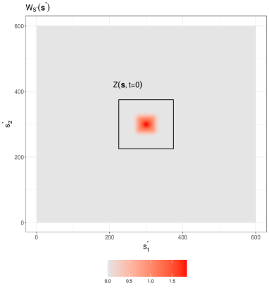
Figure 1: Large image $W_{S^{*}}(\mathbf{s}^{*})$ on grid $\mathcal{G}^{*}$ and $X_{S}(\mathbf{s})=Z(\mathbf{s},0)$, the starting point for our simulations, on grid $\mathcal{G}$, delimited by black solid segments.

Our first example is the classical frozen field with constant velocity, shown in Figure 2. Here the every spatial location $\mathbf{s}$ is transported exactly by deterministic velocity $\mathbf{v}=(10,0)^{T}$ at every time point.

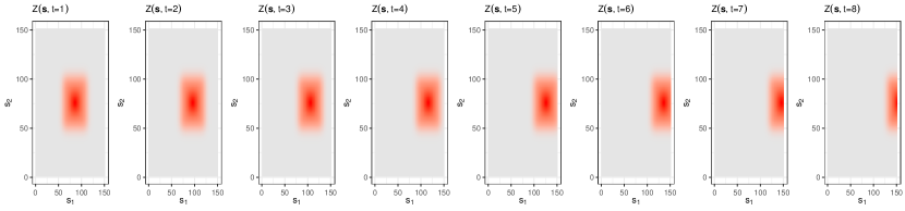
Figure 2: Classic frozen field simulation with $\mathbf{v}=(10,0)^{T}$.

We now simulate traveling fields starting from the same spatial spectrum $S_{XX}^{(S)}(\mathbf{k})=\lVert\mathbf{k}\rVert^{-\alpha}$, namely a powerlaw spectrum such as in [40], and show how different specifications of $S_{ZZ}(\mathbf{k},\omega)$ behave. Some care needs to be applied when generating such fields as fBm is not stationary, and with a powerlaw, a decay that is integrable near zero frequency is not integrable at high frequencies. The first idea might be to use a powerlaw for a range of frequencies, but it should be noted that does not strictly correspond to the spectrum of a sampled stochastic process with a powerlaw spectrum, see also discussion in [2] and [34]. We have chosen here to ignore the discrepancy between the sampled fBm and the idealized powerlaw.

We choose $\alpha=5$ for all simulations of the traveling random fields along $t=0,\dots,4$. Moreover, we pick persistence parameter $\delta=2$ and velocity $\mathbf{v}=(10,0)^{T}$. We compare the orientationally persistent frozen field realization with those from damped and frequency-dependent damped frozen fields, (10) and (11) respectively. We choose damping parameters $h=1$ for the former, and $a=1$ for the latter. The choice of these parameters is arbitrary, and we selected values that are large enough to bring a damping effect without disrupting the overall geometry of the realization. Figure 3 shows our reference orientationally persistent frozen field in the first row, and the damped and frequency-dependent damped counterparts in the second and third rows, respectively.

We notice that, compared to the orientationally persistent frozen field realization, the frequency-dependent damped frozen field looks much smoother, while preserving the same range of values. On the contrary, the damped frozen field realization takes values that are re-scaled of almost an order $10^{2}$. This is not surprising, as the damping in the damped frozen field model acts in the same way across all frequencies. In the supplementary materials we further compare the process in the first row of Figure 3, framed in red as it is taken as “reference” realization, with other orientationally persistent frozen field realizations obtained by changing either $\delta$ or $\mathbf{v}$ at a time.

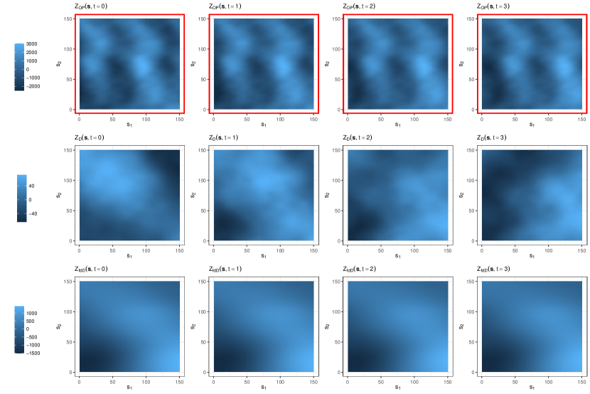
Figure 3: Orientationally persistent frozen field (first row), damped frozen field with $h=1$ (second row) and frequency-dependent damped frozen field with $a=1$ (third row). The magnitude of the values of each one of the traveling fields are indicated in the legends on the left.

Heterogeneous frozen fields

First of all, we show two examples of distributed frozen fields. In the first one we select a deterministic “preferential” velocity $\mathbf{v}$ and then draw phases and amplitudes that are similar, but not the same, as those of $\mathbf{v}$. More specifically, phases are drawn from

$$\theta_{1},\dots,\theta_{n_{\text{v}}}\stackrel{{\scriptstyle iid}}{{\sim}}f_{P}(\theta;\bm{\alpha}_{P}),$$ (19)

where $\theta=\mathrm{angle}(\mathbf{v})$ and $\theta_{i}=\mathrm{angle}(\mathbf{v}_{i})$, and amplitudes from

$$||\mathbf{v}_{1}||,\dots,||\mathbf{v}_{n_{\text{v}}}||\stackrel{{\scriptstyle iid}}{{\sim}}f_{A}(||\mathbf{v}||;\bm{\alpha}_{A}),$$ (20)

In (19) and (20) we indicate with $f_{P}$ and $f_{A}$ the distributions of the phase (P) and amplitude (A) components, with corresponding parameters $\bm{\alpha}_{P}$ and $\bm{\alpha}_{A}$, respectively. Hence, the resulting velocities are

$$\mathbf{v}_{i}=(||\mathbf{v}_{i}||\mathrm{cos}(\theta_{i}),||\mathbf{v}_{i}||\mathrm{sin}(\theta_{i}))^{T},\hskip 14.22636pti=1,\dots,{n_{\text{v}}}.$$ (21)

As for the weights in the linear combination (14), we can choose the products of probabilities

$$p_{i}=F_{P}(\theta_{i})F_{A}(||\mathbf{v}_{i}||),\hskip 14.22636pti=1,\dots,{n_{\text{v}}},$$ (22)

where $F_{P}$ and $F_{A}$ indicate the CDFs corresponding to $f_{P}$ and $f_{A}$, respectively, and make the mutatis mutandis changes in three dimensions. The above procedure only implies a pure translation of space random field according to the discrete set of velocities described in (21). The traveling random field shown in Figure 4 was generated by choosing $\mathbf{v}=(10,0)^{T}$, and we draw $n_{\text{v}}=10$ phase and amplitude components as in (19) and (20). We set $\theta_{1},\dots,\theta_{n_{\text{v}}}\stackrel{{\scriptstyle iid}}{{\sim}}\mathcal{WN}(\theta,(0.5)^{2})$, where $\mathcal{WN}$ indicates a wrapped Gaussian distribution [16], and $||\mathbf{v}_{1}||,\dots,||\mathbf{v}_{n_{\text{v}}}||\stackrel{{\scriptstyle iid}}{{\sim}}\mathcal{N}(||\mathbf{v}||,2^{2})$.

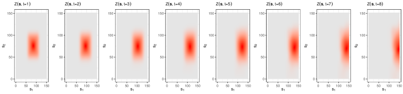
Figure 4: Distributed frozen field simulation obtained by linear combination of preferential velocity $\mathbf{v}=(10,0)^{T}$ and velocities whose phase and amplitude components are drawn randomly.

We now turn to an example where random components are drawn at every time point. In particular, given a fixed $t=1,\dots,T$, we are interested in combining rotation and translation of the random field by means of

$$\theta_{1}^{t},\dots,\theta_{n_{\theta}}^{t}\stackrel{{\scriptstyle iid}}{{\sim}}f_{R}(\theta;\bm{\alpha}_{R}),$$ (23)

and

$$\mathbf{v}^{t}\sim f_{T}(\mathbf{v};\bm{\alpha}_{T}).$$ (24)

Equation (23) denotes the $n_{\theta}$ angles drawn at every $t$ which define all the directions in which grid $\mathcal{G}$ is rotated. We denote with $X^{\theta^{t}_{i}}_{S}$ the (anticlockwise) rotated $X_{S}$ by $\theta^{t}_{i}$ around a center of rotation $C^{t}$. On the other hand, equation (24) describes velocity $\mathbf{v}^{t}$ with which all the field travels at time $t$. Then, for fixed $t$, we obtain the distributed frozen field as

$$Z(\mathbf{s},t) =\sum_{i=1}^{n_{\theta}}p(\theta^{t}_{i})X^{\theta^{t}_{i}}_{S}(\mathbf{s}-\mathbf{v}^{t}t),$$ (25)

where $p(\theta^{t}_{i})=F_{R}(\theta^{t}_{i})$, for $i=1,\dots,n_{\theta}$. In the upper panels of Figure 5 we show an example of such distributed frozen field with $n_{\theta}=20$, and for every $t=1,\dots,T$ we take $\theta^{t}_{1},\dots,\theta^{t}_{n_{\theta}}\stackrel{{\scriptstyle iid}}{{\sim}}\mathcal{WN}(0,5^{2})$ and $\mathbf{v}^{t}\sim\mathcal{N}(\bm{\mu},\mathbb{I})$, with $\bm{\mu}=(5,0)^{T}$. The centres of rotation $C^{t}$ are such that

$$C^{t}=C^{0}-\mathbf{v}^{t}t,$$

where $C^{0}=(75,105)^{T}$, and they are shown with a black dot.

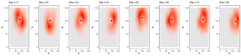
Figure 5: Distributed frozen field simulation with respective centres of rotation $C^{t}$ represented as a black dot.

We now wish to simulate evolving frozen fields. We show an example in which velocity field $\mathbf{v}(\mathbf{s},t)$ is such that

$$\mathbf{v}(\mathbf{s},t)=\left(\frac{R(\mathbf{s})\cdot\text{cos}(t)}{t+1},\frac{R(\mathbf{s})\cdot\text{sin}(t)}{t+1}\right)^{T},$$ (26)

with

$$R(\mathbf{s})=\frac{||\mathbf{s}||}{2}.$$

Such velocity field describes a spiral whose radius $R(\mathbf{s})$ changes at each spatial location. Hence, the magnitude of the point-wise elements of the velocity field depends on both the location and the time, while their direction only on the latter. In the top and bottom rows of Figure 6 we show the traveling field and the corresponding velocity fields changing over time, respectively. Notice that the velocity fields have been re-scaled for representation purposes.

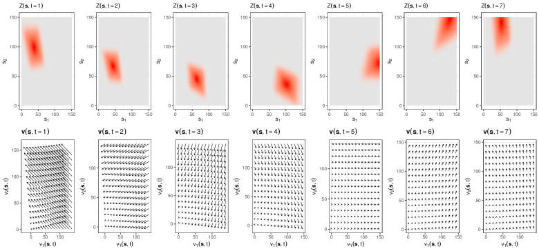
Figure 6: Evolving frozen field simulation with (top row) and the corresponding velocity filed $\mathbf{v}(\mathbf{s},t)$ at every time point (bottom row).

3.2 Computational speed

Simulation of space-time phenomena can come at an extreme computational expense. First of all, one encounters the taxing chore of enumerating the sample covariance function in a sensible way. This is not an easy task, especially for models requiring non-separable covariance.

Then, say we wish to simulate a space random field defined on square grid $\mathcal{G}=[0,n]\times[0,n]$ traveling in time at epochs $t=0,\dots,T$ as in the examples shown. An exact simulation would involve the decomposition, for instance Cholesky, of the sample covariance function, requiring a cost of order $\mathcal{O}(n^{6}T^{3})$; for Toeplitz matrices faster inversions are possible [29], but in space-time the structure is not as simple as in 1-dimensional domain such as time. Circulant embedding (see for instance [5] [13], [18]) is a less expensive and by far one of the most popular algorithms to generate realizations of space and space-time phenomena. Using such method for the traveling random fields would require a computational cost of $\mathcal{O}\left(n^{4}T^{2}\left[\log(n)+\log(T)\right]\right)$ due to performing 3-dimensional Fast Fourier Transform (FFT) twice.

In the examples shown above, we simulated orientationally preserving, damped and frequency-dependent damped frozen fields via Davis-Harte algorithm, see [33]. Such method requires computational complexity comparable to that of circulant embedding, since it involves carrying out a 3-dimensional FFT once, and is approximate, not exact.

However, all the other realizations were created relying on our proposed method. In particular, to simulate a Gaussian space random field traveling in time, we would first simulate the larger space random field on grid $\mathcal{G}^{*}=[0,N]\times[0,N]$ with circulant embedding at cost $\mathcal{O}\left(N^{4}\log(N)\right)$, and then shift the smaller $n\times n$ traveling space random fields according to the chosen velocity for a total of $T$ times, at cost $\mathcal{O}\left(T\right)$. An upper bound for $N$ is

$$n+T\text{v}_{\text{max}},$$

where $\text{v}_{\text{max}}=\max\{\text{v}_{1},\text{v}_{2}\}$ for deterministic $\mathbf{v}=(\text{v}_{1},\text{v}_{2})^{T}$, and $\text{v}_{\text{max}}=\max\{\lVert\text{v}_{1}\rVert_{\infty},\lVert\text{v}_{2}\rVert_{\infty}\}$ for varying velocity $\mathbf{v}(\mathbf{s},t)=(\text{v}_{1}(\mathbf{s},t),\text{v}_{2}(\mathbf{s},t))^{T}$, where we determine $\lVert\text{v}_{i}\rVert_{\infty}=\inf\{V\geq 0:|\text{v}_{i}|\leq V\text{ for a.e. }(\mathbf{s},t)\}$, $i=1,2$. Moreover, for distributed velocity $\mathbf{v}\sim f(\bm{\mu},\Sigma)$ we use a high percentile of such as $95\%$, namely $\mathbf{v}^{95}=(\text{v}^{95}_{1},\text{v}^{95}_{2})$, to get $\text{v}_{\text{max}}=\max\{\text{v}^{95}_{1},\text{v}^{95}_{2}\}$. Hence, in the worst case scenario, our method has a computational complexity of $\mathcal{O}\left((n^{4}+T^{4})\log(n+T)\right)$. It is then straightforward that our proposed method is much more computationally efficient than circulant embedding for simulation of space-time phenomena.

4 Conclusions

The curse of dimensionality [1] is especially problematic for stochastic processes in higher dimensions. The rationale is that even for Gaussian processes unless the covariance function is assumed to be compact or separable across dimensions, enumerating the cross-covariances between points in different dimensions scales badly once we consider space-time. Simulation is especially problematic, as even if we assume that we study Gaussian processes, enumerating the covariance matrix is not an efficient operation. Even based on spectral representations, we quickly ground to a halt in increasing dimensions.

Studying recent spatio-temporal papers, see for example [7, 35] for a review as well as the references in [36], separability is still a key feature of interest, as is isotropy in space. Mechanisms that build on how phenomena travel across space in time, have lead to the plane-wave and frozen field models. Our aim in this manuscript is to model advection in space-time more flexibly and to simulate non-separable spatio-temporal phenomena. We build on the frozen field representation and proposed new models that can be generated efficiently.

In particular, we have proposed a plethora of flexible models for both homogeneous and heterogeneous traveling fields, merging tools from statistics, spectral analysis and continuum mechanics. We showed examples of realizations of such traveling phenomena as well, and discussed how the proposed simulation methods are more or as computationally efficient as other algorithms [4, 28] from the literature of space-time random fields generation. Our computational gains follow from us proposing a method that is attuned to the nature of the observations, exploiting any inherent geometry in the stochastic process.

5 Acknowledgements

Sofia Olhede would like to thank the European Research Council under Grant CoG 2015-682172NETS, within the Seventh European Union Framework Program.

References

- [1] Richard E Bellman and Stuart E Dreyfus. Applied dynamic programming, volume 2050. Princeton university press, 2015.
- [2] Johannes Bruining, Diederik van Batenburg, Larry W Lake, and An Ping Yang. Flexible spectral methods for the generation of random fields with power-law semivariograms. Mathematical Geology, 29:823–848, 1997.
- [3] G. H. Bryan, R. P. Worsnop, J. K. Lundquist, and J. A. Zhang. A simple method for simulating wind profiles in the boundary layer of tropical cyclones. Boundary-layer meteorology, 162:475–502, 2017.
- [4] G. Chan and A. T. A. Wood. Simulation of stationary Gaussian vector fields. Statistics and computing, 9(4):265–268, 1999.
- [5] Grace Chan and Andrew T.A. Wood. Algorithm as 312: An algorithm for simulating stationary gaussian random fields. Journal of the Royal Statistical Society: Series C (Applied Statistics), 46(1):171–181, 1997.
- [6] S. Chen and R. H. Kraichnan. Simulations of a randomly advected passive scalar field. Physics of Fluids, 10(11):2867–2884, 1998.
- [7] W. Chen, M. G. Genton, and Y. Sun. Space-time covariance structures and models. Annual Review of Statistics and Its Application, 8:191–215, 2021.
- [8] G. Christakos. Spatiotemporal random fields: theory and applications. Elsevier, 2017.
- [9] George Christakos, Chutian Zhang, and Junyu He. A traveling epidemic model of space–time disease spread. Stochastic Environmental Research and Risk Assessment, 31(2):305–314, 2017.
- [10] J. H. Conway, R. T. Curtis, S. P. Norton, R. A. Parker, and R. A. Wilson. Finite groups, 1985.
- [11] D. R. Cox and Valerie Isham. A simple spatial-temporal model of rainfall. Proceedings of the Royal Society of London. Series A, Mathematical and Physical Sciences, 415(1849):317–328, 1988.
- [12] J. J. Derksen and H. E. A. Van den Akker. Simulation of vortex core precession in a reverse-flow cyclone. AIChE Journal, 46(7):1317–1331, 2000.
- [13] C. R. Dietrich and G. N. Newsam. Fast and exact simulation of stationary gaussian processes through circulant embedding of the covariance matrix. SIAM Journal on Scientific Computing, 18(4):1088–1107, 1997.
- [14] Kie B Eom. Long-correlation image models for textures with circular and elliptical correlation structures. IEEE transactions on image processing, 10(7):1047–1055, 2001.
- [15] Lawrence C. Evans. Partial differential equations. American Mathematical Society, Providence, R.I., 2010.
- [16] N. I. Fisher. Statistical analysis of circular data. cambridge university press, 1995.
- [17] J. A. Goff and T. H. Jordan. Stochastic modeling of seafloor morphology: Inversion of sea beam data for second-order statistics. Journal of Geophysical Research: Solid Earth, 93(B11):13589–13608, 1988.
- [18] I. G. Graham, F. Y. Kuo, D. Nuyens, R. Scheichl, and I. H. Sloan. Analysis of circulant embedding methods for sampling stationary random fields. SIAM Journal on Numerical Analysis, 56(3):1871–1895, 2018.
- [19] A. P. Guillaumin, A. M. Sykulski, S. C. Olhede, and Frederik J Simons. The debiased spatial Whittle likelihood. J. Roy. Stat Soc b, 84(4), 2019.
- [20] J. Guinness. Permutation and grouping methods for sharpening gaussian process approximations. Technometrics, 60(4):415–429, 2018.
- [21] J. Guinness. Nonparametric spectral methods for multivariate spatial and spatial–temporal data. Journal of Multivariate Analysis, 187:104823, 2022.
- [22] Joseph Guinness and Montserrat Fuentes. Circulant embedding of approximate covariances for inference from gaussian data on large lattices. Journal of computational and Graphical Statistics, 26(1):88–97, 2017.
- [23] D. Horntrop and A. Majda. An overview of monte carlo simulation techniques for the generation of random fields. Monte Carlo Simulations in Oceanography, pages 67–79, 1997.
- [24] Lance M Kaplan and C-CJ Kuo. An improved method for 2-d self-similar image synthesis. IEEE transactions on image processing, 5(5):754–761, 1996.
- [25] P.K. Kundu, I.M. Cohen, and D.R. Dowling. Fluid Mechanics. Academic Press. Academic Press, 2015.
- [26] F. Lavancier. Long memory random fields. Dependence in probability and statistics, pages 195–220, 2006.
- [27] J. M. Lilly, A. M. Sykulski, J. J. Early, and S. C. Olhede. Fractional brownian motion, the matérn process, and stochastic modeling of turbulent dispersion. Nonlinear Processes in Geophysics, 24(3):481–514, 2017.
- [28] A. Mantoglou and J. L. Wilson. The turning bands method for simulation of random fields using line generation by a spectral method. Water Resources Research, 18(5):1379–1394, 1982.
- [29] P.-G. Martinsson, V. Rokhlin, and M. Tygert. A fast algorithm for the inversion of general toeplitz matrices. Computers & Mathematics with Applications, 50(5-6):741–752, 2005.
- [30] S. Most, D. Bolster, B. Bijeljic, and Wolfgang Nowak. Trajectories as training images to simulate advective-diffusive, non-fickian transport. Water Resources Research, 55(4):3465–3480, 2019.
- [31] S. C. Olhede, E. J. McCoy, and D. A. Stephens. Large-sample properties of the periodogram estimator of seasonally persistent processes. Biometrika, 91(3):613–628, 2004.
- [32] S. M. Papalexiou, F. Serinaldi, and E. Porcu. Advancing space-time simulation of random fields: From storms to cyclones and beyond. Water Resources Research, 57(8):e2020WR029466, 2021.
- [33] D. B. Percival. Simulating Gaussian random processes with specified spectra. Comp. Sc. Stat., 24:534– 538, 1992.
- [34] Donald B Percival and Andrew T Walden. Wavelet methods for time series analysis, volume 4. Cambridge university press, 2000.
- [35] Emilio Porcu, Reinhard Furrer, and Douglas Nychka. 30 years of space–time covariance functions. Wiley Interdisciplinary Reviews: Computational Statistics, 13(2):e1512, 2021.
- [36] M. L. O. Salvaña, A. Lenzi, and M. G. Genton. Spatio-temporal cross-covariance functions under the Lagrangian framework with multiple advections. Journal of the American Statistical Association, TBA(Accepted):1–30, 2022.
- [37] M. Schlather. Some covariance models based on normal scale mixtures. Bernoulli, 16(3):780–797, 2010.
- [38] M. Schlather. Construction of covariance functions and unconditional simulation of random fields. In Advances and challenges in space-time modelling of natural events, pages 25–54. Springer, 2012.
- [39] M. L. Stein. Interpolation of spatial data: some theory for kriging. Springer Science & Business Media, 1999.
- [40] Michael L Stein. Fast and exact simulation of fractional brownian surfaces. Journal of Computational and Graphical Statistics, 11(3):587–599, 2002.