A systematic perturbative expansion of the solution of the time-independent Gross-Pitaevskii equation

Abstract

In this article a perturbative solution of the Gross-Pitaevskii(GP) equation in the $D$-dimensional space $R^{D}$ with a general external potential is studied. The solution describes the condensate wave-function of a gas containing $N$ Bose particles. A criteria for the validity of the perturbative solution is developed. Furthermore expressions for the particle density, the chemical potential, the internal energy and the mean-square radius of the condensate are derived corrected to first order in the coupling constant. The scheme is then applied to obtain the solution of the GP equation in $D=1,2,3$ for external harmonic potentials. It is shown, in each case, that if $N$ exceeds a certain value the solution breaks down.

1 Introduction

The long awaited experimental realization of Bose-Einstein condensation(BEC) in 1995 [1, 2, 3] has sparked a huge interest in studying the properties of the newly formed phase and its dynamics. The order parameter of this phase transition and the dynamics of BEC are most accurately described near zero temperature for weak inter-particle interactions by a cubic nonlinear Schrödinger equation with an external potential, namely the Gross-Pitaevskii(GP) equation [4, 5, 6, 7, 8, 9, 10, 11, 12]. The external potential represents the trapping potential and the nonlinear term describes, within the mean field approximation, the inter-particle interactions which maybe repulsive or attractive. The GP equation has applications in nonlinear phenomena as in nonlinear optics [13, 14, 15, 16], gravitational physics [17, 18, 19, 20], the Josephson effect [21, 22] and in condensed matter physics [23].

Due to its diverse applications in various branches of physics, immense theoretical efforts have been dedicated towards solving the GP equation which seems to be non-integrable even in one dimension. This is due to the presence of the external potential. To overcome this difficulty several approaches were developed which may be divided into numerical and analytical methods. The analytical methods can further be divided into exact solutions for particular forms of the external potential and approximate solutions in analytical forms.

The first approach is to develop numerical techniques to solve both of the time-dependent and time-independent GP equation. We shall briefly mention some widely used numerical methods, for a detailed review see [24] and references therein. Several methods were adapted to solve numerically the time-independent GP equation. The variational scheme was used by Bao and Tang [25] to solve the GP equation for different forms of the external potential. The boundary-eigenvalue method was applied by Edwards and Burnett [26] to obtain solutions of the three-dimensional GP equation with spherically symmetric potentials. Adhikari [27, 28] used the same technique to obtain the ground state solution of the GP equation in two dimensions with a radially symmetric potential. Another efficient technique, based on simulation of the evolution equation in imaginary time through a Wick rotation, was applied by Chiofalo et al [29] to compute the ground state solution of BEC in a one-dimensional optical lattice with a superimposed harmonic trap.

For the time-dependent GP equation several schemes were also developed. Cerimele [30] et al used a synchronized scheme to solve the two-dimensional GP equation with cylindrical symmetry. Time-dependent extensions of the boundary-eigenvalue method were also developed by Adhikari [31] to solve the axially-symmetric two-dimensional GP equation. Muruganandam and Adhikari [32] used a pseudo-spectral method combined with a Runge-Kutta marching scheme to solve the GP equation in three dimensions. Another widely used technique is the time-splitting spectral method used by Bao et al [33] to solve the GP equation in one, two and three dimensions for weak as well as strong external potentials. A review of other popular methods is also listed in [34].

The second approach is to develop methods for constructing particular solutions for the GP equation in an analytical form. A family of stationary periodic solutions to the one-dimensional GP equation with a specifically devised periodic potential was obtained for repulsive interactions by Carr et al [35] and Bronski et al [36] and also for attractive potentials [37, 38]. Hua-Mei [39] used the mapping method to find exact solutions of the one-dimensional time-dependent GP equation with a magnetic trap. He obtained bright and dark soliton solutions and soliton-like solutions. Similarity transformations were used by Belmonte-Beitia et al [40] to map a one-dimensional time-dependent GP equation with specific time-dependent potentials to a one-dimensional stationary nonlinear Schrödinger equation (NLS). Various solutions were constructed including breathers, resonant solitons and quasi-periodic solitons. They also applied the same technique to construct periodic solutions for the time-independent GP equation with periodic potentials and space-dependent coupling constant [41]. The same approach was applied by Yu [42] to obtain families of exact solutions for the time-dependent GP equation in three dimensions with space- and time-dependent coupling constant. Malomed and Stepanyants [43] used the known solutions of the Gardner equation to generate a family of stationary solutions to the GP equation. They also applied the inverse problem to construct potential functions which support solutions relevant to a particular physical system. The modified Kudryashev method was also used by Neirameh [44] to obtain solutions of the time-dependent GP equation. Liu et al [45] constructed classes of exactly solvable stationary GP equations with variable coefficients, using transformations to a GP equation with a known exact solution.

A subclass of the analytical methods is to develop approximate solutions for the GP equation in analytical forms. Belonging to this class is the Thomas-Fermi approximation introduced by Baym and Pethick [46]. Another approach is to apply the variational method with trial functions which are usually Gaussian or solitonic to reduce the problem to a system of ordinary differential evolution equations for some free parameters [47, 48].

Another approach belonging to this subclass is to apply perturbation theory in the limit of a weak nonlinear interaction. The solution strategy starts with the general solution of an effective one-dimensional GP equation with a harmonic oscillator potential which is then expressed as a series expansion in terms of the solutions of its linear counterpart. The coefficients of the expansion could then be sought for using various methods. Kivshar et al [49] obtained a system of algebraic equations for the coefficients which they solved, within the weak nonlinearity limit, for the ground state mode as well as for the higher order modes. Trallero-Giner et al [50] obtained for the coefficients a system of nonlinear algebraic equations by transforming the GP equation into an integral equation using the Green’s function of the linear operator, whose spectral representation is given in terms of the one-dimensional harmonic oscillator wave-functions. The algebraic system was solved using the iterative method and also using the perturbative method in the weak nonlinearity limit. Shi et al [51] approached the same problem using the homotopy analysis method where a homotopy is constructed with an embedding parameter that goes from zero, corresponding to the linear case, to one, corresponding to the nonlinear GP equation. Assuming that in between those extremes the solution varies smoothly as a function of the embedding parameter, a Maclaurin series is constructed with respect to the embedding parameter for the solution. A set of recursive linearized equations is obtained, which is solved using the Galerkin method. Jia-Ren et al [52] studied the perturbative solutions of the GP equation in three dimensions with a spherically symmetric harmonic trap. They expressed the results in terms of the Hermite polynomials and compared their results with the numerical solutions of the GP equation.

In this paper we will generalize the approach used in reference [50] for an arbitrary external potential and in an arbitrary dimension. The method is then applied to obtain solutions of the GP equation in one dimension, two dimensions with a rotationally-symmetric and three dimensions with a spherically-symmetric potential. The organization of the paper is as follows. In Section 2 the GP equation in the D-dimensional space $R^{D}$ with an arbitrary external potential is transformed into a system of coupled nonlinear integral equations. In Sections 3 and 4 the integral equations are solved successively and the expansion coefficients are determined as well as the corresponding chemical potentials, furthermore the physical interpretation of the normalization condition is discussed. In Section 5 the particle density, the internal energy and the mean-square radius of the condensate are calculated. The method is then applied in Sections 6, 7 and 8 to study the GP equation in one dimension, two dimensions with rotational symmetry and three dimensions with spherical symmetry. In Section 9 we summarize the obtained results and discuss future prospects.

2 Formulation of the problem

We consider a gas of $N$ identical Bose particles, each of mass ${m}_{b}$, in an external potential $V_{ext}(\vec{r})$, where $\vec{r}$ is the position vector in the $D$-dimensional space ${R}^{D}$. The gas is assumed to be in a state of thermodynamic equilibrium at zero temperature. The energy of the stationary condensate $\psi(\vec{r})$ is given by the energy functional [11] page 148:

$$E[{\psi^{*}},\psi]=\int{{d^{D}}r}\,\{\frac{{{\hbar^{2}}}}{{2{m_{b}}}}|{\vec{\nabla}_{D}}\psi(\vec{r}){|^{2}}+{V_{ext}}(\vec{r})|\psi(\vec{r}){|^{2}}+\frac{g_{D}}{2}{[|\psi(\vec{r}){|^{2}}]^{2}}\},$$ (1)

where ${\vec{\nabla}_{D}}$ is the gradient operator in ${R}^{D}$ and ${g_{D}}$ is the coupling constant which is given for $D=3$ by [11] page 114:

$${g_{3}}\equiv g=\frac{{4\pi a{\hbar^{2}}}}{{{m_{b}}}}$$ (2)

Here a is the s-wave scattering length. The appropriate expressions for $g_{1}$ and $g_{2}$ are given in Section 6 and Section 7 respectively.

If the external potential $V_{ext}(\vec{r})$ is continuous and approaches infinity as $|\vec{r}|\to\infty$ and if $g_{D}>0$ then the energy functional is convex and its minimum gives the ground state of the Bose condensate $\psi(\vec{r})$. In addition $\psi(\vec{r})$ is unique up to a global phase which can always be chosen such that it is real valued and positive [53]. On the other hand if $g_{D}<0$ the ground state exists only at low coupling constants and for a limited number of Bosons in $V_{ext}(\vec{r})$ as long as the minimum-energy balances the effective attraction and prevents collapse [24].

To obtain the equation of motion for the condensate wave-function $\psi(\vec{r})$, we have to minimize the energy functional Eq.(1) subject to the constraint that the total number of particles in the system is equal to $N$:

$$\int{{d^{D}}r}\,|\psi(\vec{r}){|^{2}}=N.$$ (3)

To carry out the minimization we use the method of the Lagrange multipliers. We construct the auxiliary functional:

$$\begin{gathered}K[{\psi^{*}},\psi,\mu\,]\,=\,E[{\psi^{*}},\psi]\,-\,\mu\,\int{{d^{D}}r}\,|\psi(\vec{r}){|^{2}}\hfill\\ =\int{{d^{D}}r}\,\{\frac{{{\hbar^{2}}}}{{2{m_{b}}}}|{{\vec{\nabla}}_{D}}\psi(\vec{r}){|^{2}}+[{V_{ext}}(\vec{r})-\mu]|\psi(\vec{r}){|^{2}}+\frac{g_{D}}{2}{[|\psi(\vec{r}){|^{2}}]^{2}}\},\hfill\\ \end{gathered}$$ (4)

where the chemical potential $\mu$ is the Lagrange multiplier which ensures the constancy of the number of particles. The equation of motion of the condensate wave-function is then

$$\frac{{\delta K[{\psi^{*}},\psi,\,\mu]}}{{\delta{\psi^{*}}(\vec{r})}}=0$$ (5)

Inserting Eq.(4) into Eq.(5) we obtain the Gross-Pitaevskii(GP) equation:

$$[-\frac{{{\hbar^{2}}}}{{2{m_{b}}}}{{\vec{\nabla}}^{2}}_{D}+{V_{ext}}(\vec{r})-\mu+g_{D}|\psi(\vec{r}){|^{2}}]\,\psi(\vec{r})=0.$$ (6)

We shall consider perturbative solutions of the GP equation for the special case $g_{D}>0$, and assume that the chemical potential $\mu$ depends on the coupling constant:

$$\mu=\mu(g_{D})$$ (7)

Furthermore we assume that the problem recommends a characteristic length ${l_{c}}$ from which we can define a characteristic angular frequency ${\omega_{c}}$ by:

$${\omega_{c}}=\frac{\hbar}{{{m_{b}}\,{l_{c}}^{2}}}$$ (8)

Using $l_{c}$ and ${\omega_{c}}$ we can define the dimensionless quantities:

$$\vec{\xi}=\frac{{\vec{r}}}{{{l_{c}}}};\,\,\,\,\,\,\,\tilde{\mu}=\frac{\mu}{{\hbar\,{\omega_{c}}\,}}\,\,\,\,\,\,\,and\,\,\,\,\,\,\,\tilde{g}_{D}=l_{c}^{-D}\frac{g_{D}}{{\hbar\,{\omega_{c}}}}$$ (9)

and the dimensionless condensate wave-function:

$$\tilde{\psi}=l_{c}^{\frac{D}{2}}\,\psi.$$ (10)

In terms of the dimensionless quantities the GP equation takes the form:

$$[-\frac{1}{2}{{\vec{\nabla}}^{2}}_{\xi}+{{\tilde{V}}_{ext}}(\vec{\xi})-\tilde{\mu}+\tilde{g}_{D}|\tilde{\psi}(\vec{\xi}){|^{2}}]\,\tilde{\psi}(\vec{\xi})=0$$ (11)

We introduce the linear differential operator:

$${L_{\xi}}=-\frac{1}{2}\,{{\vec{\nabla}}^{2}}_{\xi}\,\,+\,\,{{\tilde{V}}_{ext}}(\vec{\xi}),$$ (12)

and rearrange Eq.(10) in the form:

$${L_{\xi}}\,\tilde{\psi}(\vec{\xi})=[\,\tilde{\mu}-\tilde{g}|\tilde{\psi}(\vec{\xi}){|^{2}}]\,\,\tilde{\psi}(\vec{\xi})$$ (13)

Let G be the Green’s function of the differential operator ${L_{\xi}}$:

$${L_{\xi}}\,G\,(\,\vec{\xi},\,\vec{\eta}\,)\,=\,{\delta^{D}}(\,\vec{\xi}-\vec{\eta}\,),$$ (14)

where ${\delta^{D}}(\,\vec{\xi}-\vec{\eta}\,)$ is the D-dimensional Dirac-delta function. The condensate wave-function $\tilde{\psi}(\vec{\xi})$ satisfies the nonlinear integral equation:

$$\tilde{\psi}(\vec{\xi})=\int{{d^{D}}\eta\,\,G\,(\,\vec{\xi},\,\vec{\eta}\,)\,[\,\tilde{\mu}-\tilde{g}_{D}|\tilde{\psi}(\vec{\eta}){|^{2}}]\,\,\tilde{\psi}(\vec{\eta})}.$$ (15)

We solve the integral equation (15) using the small parameter method [54]. We assume that the condensate wave-function is non-degenerate and expand $\tilde{\mu}\,(\tilde{g})$ and $\tilde{\psi}(\vec{\xi},\tilde{g})$ in a power series in ${\tilde{g}}$:

$$\tilde{\mu}\,(\tilde{g}_{D})\,=\sum\limits_{n\,=\,0}{\,{{\tilde{g}_{D}}^{n}}}\,{{\tilde{\mu}}_{n}},\,\,\,\,\,\,and\,\,\,\,\,\,\tilde{\psi}(\vec{\xi},\tilde{g}_{D})\,=\sum\limits_{n\,=\,0}{\,{{\tilde{g}_{D}}^{n}}}\,{{\tilde{\psi}}^{(n)}}(\vec{\xi})$$ (16)

We substitute Eq.(16) into Eq.(15) and use the fact that the condensate wave-function is real, we arrive at:

$$\begin{gathered}{{\tilde{\psi}}^{(0)}}(\vec{\xi})\,+\,\tilde{g}_{D}\,{{\tilde{\psi}}^{(1)}}(\vec{\xi})+{{\tilde{g}_{D}}^{2}}\,{{\tilde{\psi}}^{(2)}}(\vec{\xi})+...=\,{{\tilde{\mu}}_{0}}\int{{d^{D}}\eta\,\,G\,(\,\vec{\xi},\,\vec{\eta}\,)\,\,{{\tilde{\psi}}^{(0)}}(\vec{\eta})}\hfill\\ +\,\tilde{g}_{D}\,\int{{d^{D}}\eta\,\,G\,(\,\vec{\xi},\,\vec{\eta}\,)\,[{{\tilde{\mu}}_{1}}\,\,{{\tilde{\psi}}^{(0)}}(\vec{\eta})\,+}\,{{\tilde{\mu}}_{0}}\,\,{{\tilde{\psi}}^{(1)}}(\vec{\eta})\,-\,{{\tilde{\psi}}^{(0)\,3}}(\vec{\eta})\,]\hfill\\ +{{\tilde{g}_{D}}^{2}}\int{{d^{D}}\eta\,\,G\,(\,\vec{\xi},\,\vec{\eta}\,)\,[{{\tilde{\mu}}_{2}}\,\,{{\tilde{\psi}}^{(0)}}(\vec{\eta})\,+}\,{{\tilde{\mu}}_{1}}\,\,{{\tilde{\psi}}^{(1)}}(\vec{\eta})+{{\tilde{\mu}}_{0}}\,\,{{\tilde{\psi}}^{(2)}}(\vec{\eta})\,\,-\,3\,{{\tilde{\psi}}^{(0)\,2}}(\vec{\eta})\,{{\tilde{\psi}}^{(1)}}(\vec{\eta})\,]\hfill\\ +...\hfill\\ \end{gathered}$$ (17)

Equating the coefficients of similar powers of $\tilde{g}_{D}$ on both sides of Eq.(17) we obtain the equations:

$${{\tilde{\psi}}^{(0)}}(\vec{\xi})\,=\,{{\tilde{\mu}}_{0}}\int{{d^{D}}\eta\,\,G\,(\,\vec{\xi},\,\vec{\eta}\,)\,\,{{\tilde{\psi}}^{(0)}}(\vec{\eta})}$$ (18)

$${{\tilde{\psi}}^{(1)}}(\vec{\xi})=\,\int{{d^{D}}\eta\,\,G\,(\,\vec{\xi},\,\vec{\eta}\,)\,[{{\tilde{\mu}}_{1}}\,\,{{\tilde{\psi}}^{(0)}}(\vec{\eta})\,+}\,{{\tilde{\mu}}_{0}}\,\,{{\tilde{\psi}}^{(1)}}(\vec{\eta})\,-\,{{\tilde{\psi}}^{(0)\,3}}(\vec{\eta})\,]$$ (19)

$$\,{{\tilde{\psi}}^{(2)}}(\vec{\xi})=\,\int{{d^{D}}\eta\,\,G\,(\,\vec{\xi},\,\vec{\eta}\,)\,[{{\tilde{\mu}}_{2}}\,\,{{\tilde{\psi}}^{(0)}}(\vec{\eta})\,+}\,{{\tilde{\mu}}_{1}}\,\,{{\tilde{\psi}}^{(1)}}(\vec{\eta})+{{\tilde{\mu}}_{0}}\,\,{{\tilde{\psi}}^{(2)}}(\vec{\eta})\,\,-\,3\,{{\tilde{\psi}}^{(0)\,2}}(\vec{\eta})\,{{\tilde{\psi}}^{(1)}}(\vec{\eta})\,]$$ (20)

$$etc...$$

We have replaced the GP equation by a system of coupled integral equations in ${{\tilde{\psi}}^{(0)}}(\vec{\xi}),\,\,{{\tilde{\psi}}^{(1)}}(\vec{\xi}),\,\,{{\tilde{\psi}}^{(2)}}(\vec{\xi}),\,...$ and ${{\tilde{\mu}}_{0}},\,\,{{\tilde{\mu}}_{1}},\,\,{{\tilde{\mu}}_{2}},\,...$. The first integral equation is linear in ${{\tilde{\psi}}^{(0)}}$ and shows that ${{\tilde{\psi}}^{(0)}}$ is an eigenfunction of the linear operator ${L_{\xi}}$ corresponding to the eigenvalue ${{\tilde{\mu}}_{0}}$. Solving this equation we obtain ${{\tilde{\psi}}^{(0)}}$ and ${{\tilde{\mu}}_{0}}$. Substituting these quantities back into Eq.(18) we obtain an inhomogeneous linear integral equation in ${{\tilde{\psi}}^{(1)}}$ and ${{\tilde{\mu}}_{1}}$ which can easily be solved. Continuing this process we can, in principle, obtain ${{\tilde{\psi}}^{(2)}}(\vec{\xi}),\,\,{{\tilde{\psi}}^{(3)}}(\vec{\xi}),...$ and ${{\tilde{\mu}}_{2}},\,\,{{\tilde{\mu}}_{3}},...$. This gives a perturbative solution of the GP equation to any desired order of ${\tilde{g}_{D}}$.

3 Solution of the system of integral equations

To obtain the Green’s function associated with the differential operator ${L_{\xi}}$ we have to solve the eigenvalue problem:

$${L_{\xi}}\,\chi\,(\,\vec{\xi}\,)\,=\,\lambda\chi\,(\,\vec{\xi}\,).$$ (21)

For a large class of potentials, ${V_{ext}}$, [55, 56], the eigenvalue problem 21 has a complete set of orthonormal eigenfunctions:

$$\{{\chi_{\alpha(n)}}\,(\,\vec{\xi}\,)\},$$ (22)

where $\alpha(n)$ is a complete set of indices characterizing the eigenvalues and the eigenfunctions.

$$\int{{d^{D}}\xi\,\,}{\chi^{*}}_{\alpha(n)}\,(\,\vec{\xi}\,)\,{\chi_{\alpha(k)}}\,(\,\vec{\xi}\,)\,=\,{\delta_{\alpha(n),\,\alpha(k)}}$$ (23)

$$\sum\limits_{n}{{\chi^{*}}_{\alpha(n)}\,(\,\vec{\eta}\,)\,{\chi_{\alpha(k)}}\,(\,\vec{\xi}\,)\,\,=\,{\delta^{D}}\,(}\vec{\xi}\,-\vec{\eta})$$ (24)

We will label the eigenvalues according to their magnitudes

$$0<{\lambda_{\,\alpha\,(0)}}\,<{\lambda_{\,\alpha\,(1)}}\,\leq{\lambda_{\,\alpha\,(2)}}\leq...\leq\,{\lambda_{\,\alpha\,(n)}}\leq...$$ (25)

The Green’s function associated with the differential operator can be expressed as:

$$G\,(\,\vec{\xi},\,\vec{\eta}\,)\,=\,\sum\limits_{n}{\frac{1}{{{\lambda_{\,\alpha\,(n)}}}}{\chi^{*}}_{\alpha(n)}\,(\,\vec{\eta}\,)\,{\chi_{\alpha(n)}}\,(\,\vec{\xi}\,).\,}$$ (26)

The integral equation (15) has the form:

$$\tilde{\psi}(\vec{\xi})=\int{{d^{D}}\eta\,\,G\,(\,\vec{\xi},\,\vec{\eta}\,)\,\varphi\,(\vec{\eta}\,),}$$

where

$$\varphi\,(\vec{\xi}\,)=[\,\tilde{\mu}-\tilde{g}|\tilde{\psi}(\vec{\xi}){|^{2}}]\,\,\tilde{\psi}(\vec{\xi}).$$

Since the condensate wave-function $\tilde{\psi}(\vec{\xi})$ is assumed to be square integrable and vanishes as $|\vec{\xi}|\,\to\,0$ the function $\varphi\,(\vec{\xi}\,)$ is also square integrable and vanishes as $|\vec{\xi}|\,\to\,0$. Furthermore the kernel, $G\,(\,\vec{\xi},\,\vec{\eta}\,)$, of the integral equation is Hermitian and square integrable. Therefore, according to the Hilbert-Schmidt theorem [57], the function $\tilde{\psi}(\vec{\xi})$ can be expanded in terms of the eigenfunctions (22). In particular, we can expand the functions ${{\tilde{\psi}}^{(n)}}(\vec{\xi})\,$ in terms of this set:

$${{\tilde{\psi}}^{(0)}}(\vec{\xi})\,=\,\sum\limits_{k=0}{C_{\alpha\,(k)}^{(0)}}\,{\chi_{\alpha(k)}}\,(\,\vec{\xi}\,)$$ (27)

$${{\tilde{\psi}}^{(n)}}(\vec{\xi})\,=\,C_{\alpha\,(0)}^{(0)}\,\sum\limits_{k=0}{C_{\alpha\,(k)}^{(n)}}\,{\chi_{\alpha(k)}}\,(\,\vec{\xi}\,),\,\,\,\,\,n=1,2,...$$ (28)

Substituting Eq.(27) into Eq.(18) and using the orthogonality relation (23) we obtain

$$(\,{\lambda_{\,\alpha\,(k)}}\,-\,{{\tilde{\mu}}_{0}})\,C_{\alpha\,(k)}^{(0)}\,=\,0$$

This equation shows that $\tilde{\mu}_{0}$ is equal to one of the eigenvalues of the linear operator $L_{\xi}$, say $k=m$. Then

$$\begin{gathered}{{\tilde{\mu}}_{0}}\,=\,{\lambda_{\,\alpha\,(m)}},\,\,and\,\,\,C_{\alpha\,(m)}^{(0)}\,\neq\,0\hfill\\ C_{\alpha\,(k)}^{(0)}\,=\,0,\,\,for\,\,k\neq m\hfill\\ \end{gathered}$$ (29)

This solution is of particular importance since it represents the case in which most of the particles condense in the state ${\chi_{\alpha(m)}}$ of the trapping potential. At $T=0$ all Bose particles condense in the ground state so that $m=0$. Thus

$$C_{\alpha\,(k)}^{(0)}=\,C_{\alpha\,(0)}^{(0)}\,{\delta_{k,0}}.$$ (30)

Inserting this back into Eqs.(27) and (29), we obtain

$${{\tilde{\psi}}^{(0)}}(\vec{\xi})\,=\,C_{\alpha\,(0)}^{(0)}\,{\chi_{\alpha(0)}}\,(\,\vec{\xi}\,)$$ (31)

$${{\tilde{\mu}}_{0}}\,=\,{\lambda_{\,\alpha\,(0)}}$$ (32)

We next consider the integral equation (19). substituting Eq.(28) with $n=1$ into Eq.(19) we obtain:

$$\begin{gathered}C_{\alpha\,(0)}^{(1)}\,{\chi_{\alpha(0)}}\,(\,\vec{\xi}\,)\,+\,\sum\limits_{k\neq 0}{C_{\alpha\,(k)}^{(1)}}\,{\chi_{\alpha(k)}}\,(\,\vec{\xi}\,)\,=\,\frac{1}{{{\lambda_{\,\alpha\,(0)}}}}\,[\,{{\tilde{\mu}}_{1}}-\,C_{\alpha\,(0)}^{(0)\,2}\,{b_{\alpha\,(0)}}\,+\,{\lambda_{\,\alpha\,(0)}}\,C_{\alpha\,(0)}^{(1)\,}]\,{\chi_{\alpha(0)}}\,(\,\vec{\xi}\,)\,\hfill\\ +\,\sum\limits_{k\neq 0}{\frac{1}{{{\lambda_{\,\alpha\,(k)}}}}\,[\,-\,C_{\alpha\,(0)}^{(0)\,2}\,{b_{\alpha\,(k)}}\,+\,{\lambda_{\,\alpha\,(0)}}\,C_{\alpha\,(k)}^{(1)\,}]\,{\chi_{\alpha(k)}}\,(\,\vec{\xi}\,)\,,}\hfill\\ \end{gathered}$$ (33)

where

$${b_{\alpha\,(k)}}=\int{{d^{D}}\eta\,\,}{\chi^{*}}_{\alpha(k)}\,(\,\vec{\xi}\,)\,\chi_{\alpha(0)}^{3}\,(\,\vec{\xi}\,).$$ (34)

Equating the coefficients of the corresponding eigenfunctions on both sides gives:

$${{\tilde{\mu}}_{1}}\,=\,C_{\alpha\,(0)}^{(0)\,2}\,\,{b_{\alpha\,(0)}},\,$$ (35)

and

$$C_{\alpha\,(k)}^{(1)\,}\,=\,-\,C_{\alpha\,(0)}^{(0)\,2}\,{T_{\alpha\,(k)}};\,\,\,\,\,\,\,k\neq 0,$$ (36)

with

$${T_{\alpha\,(k)}}\,=\,\,\frac{{{b_{\alpha\,(k)}}}}{{{\lambda_{\,\alpha\,(k)}}-{\lambda_{\,\alpha\,(0)}}}};\,\,\,\,\,\,\,k\neq 0$$ (37)

To obtain ${{\tilde{\psi}}^{(2)}}$ we have to solve the integral equation(20). In this case we should take into account the change in the coupling constant $g$, due to higher order inter-particles scattering processes. This means that we have to go beyond the s-wave expression in Eq.(2). Although we will mainly be concerned with the condensate wave-function corrected to first order in g, we will go one step further and calculate the second order term to get a deeper look at the expansion and to explain how the normalization condition (3) is satisfied to all orders of the coupling constant. Substituting Eqs(28), with $n=1$ and $n=2$ into Eq.(20) we obtain

$$\begin{gathered}C_{\alpha\,(0)}^{(2)}\,{\chi_{\alpha(0)}}\,(\,\vec{\xi}\,)\,+\,\sum\limits_{k\neq 0}{C_{\alpha\,(k)}^{(2)}}\,{\chi_{\alpha(k)}}\,(\,\vec{\xi}\,)\,=\hfill\\ \,\frac{1}{{{\lambda_{\,\alpha\,(0)}}}}\,[\,{{\tilde{\mu}}_{2}}-\,3\,C_{\alpha\,(0)}^{(0)\,2}\,\,\sum\limits_{l=0}{{D_{\alpha\,(0),\alpha\,(l)}}\,C_{\alpha\,(l)}^{(1)\,}}\,+\,{{\tilde{\mu}}_{1}}\,C_{\alpha\,(0)}^{(1)\,}+{{\tilde{\mu}}_{0}}\,C_{\alpha\,(0)}^{(2)\,}]\,{\chi_{\alpha(0)}}\,(\,\vec{\xi}\,)\,\hfill\\ +\,\sum\limits_{k\neq 0}{\frac{1}{{{\lambda_{\,\alpha\,(k)}}}}\,[\,-3\,C_{\alpha\,(0)}^{(0)\,2}\,\,\sum\limits_{l=0}{{D_{\alpha\,(k),\alpha\,(l)}}\,C_{\alpha\,(l)}^{(1)\,}}\,+\,{{\tilde{\mu}}_{1}}\,C_{\alpha\,(k)}^{(1)\,}+{{\tilde{\mu}}_{0}}\,C_{\alpha\,(k)}^{(2)\,}]\,{\chi_{\alpha(k)}}\,(\,\vec{\xi}\,)\,,}\hfill\\ \end{gathered}$$ (38)

where

$${D_{\alpha\,(k),\,\alpha\,(l)}}=\int{{d^{D}}\eta\,\,}{\chi^{*}}_{\alpha(k)}\,(\,\vec{\xi}\,)\,\chi_{\alpha(0)}^{2}\,(\,\vec{\xi}\,){\chi_{\alpha\,(l)}}\,(\,\vec{\xi}\,).$$ (39)

Equating the coefficients of the corresponding eigenfunctions on both sides of Eq.(37) we obtain:

$${{\tilde{\mu}}_{2}}=3\,C_{\alpha\,(0)}^{(0)\,2}\,\,\sum\limits_{l=0}{{D_{\alpha\,(0),\alpha\,(l)}}\,C_{\alpha\,(l)}^{(1)\,}}\,-\,{{\tilde{\mu}}_{1}}\,C_{\alpha\,(0)}^{(1)\,},$$ (40)

and

$$C_{\alpha\,(k)}^{(2)}\,=\,\,\frac{1}{{{\lambda_{\,\alpha\,(k)}}}}\,[\,-3\,C_{\alpha\,(0)}^{(0)\,2}\,\,\sum\limits_{l=0}{{D_{\alpha\,(k),\alpha\,(l)}}\,C_{\alpha\,(l)}^{(1)\,}}\,+\,{{\tilde{\mu}}_{1}}\,C_{\alpha\,(k)}^{(1)\,}+{{\tilde{\mu}}_{0}}\,C_{\alpha\,(k)}^{(2)\,}],\,\,\,\,\,\,\,k\neq 0.$$ (41)

Using the results

$${D_{\alpha\,(0),\alpha\,(l)}}\,=\,\,b_{\alpha\,(k)}^{*};\,\,\,\,\,\,b_{\alpha\,(0)}^{*}={b_{\alpha\,(0)}},$$

we can express the chemical potential as:

$${{\tilde{\mu}}_{2}}=2\,C_{\alpha\,(0)}^{(0)\,2}\,C_{\alpha\,(0)}^{(1)\,}\,{b_{\alpha\,(0)}}-3\,\,C_{\alpha\,(0)}^{(0)\,4}\,\,\sum\limits_{l\neq 0}{b_{\alpha\,(l)}^{*}{T_{\alpha\,(l)}}\,}\,$$ (42)

Substituting the expressions for $C_{\alpha\,(k)}^{(1)\,}$, ${{\tilde{\mu}}_{1}}$ and ${{\tilde{\mu}}_{0}}\,$ we obtain:

$$\begin{gathered}C_{\alpha\,(k)}^{(2)}\,=\,\,-3\frac{{C_{\alpha\,(0)}^{(0)\,2}}}{{{\lambda_{\,\alpha\,(k)}}-\,\,{\lambda_{\,\alpha\,(0)}}}}\,[\,\,C_{\alpha\,(0)}^{(1)\,}\,{b_{\alpha\,(k)}}-\,\,\frac{1}{3}C_{\alpha\,(0)}^{(0)\,2}\,{b_{\alpha\,(0)}}\,{T_{\alpha\,(k)}}\hfill\\ -\,C_{\alpha\,(0)}^{(0)\,2}\,\,\sum\limits_{l\neq 0}{{D_{\alpha\,(k),\alpha\,(l)}}\,{T_{\alpha\,(l)}}}\,],\,\,\,\,\,\,\,k\neq 0\hfill\\ \end{gathered}$$ (43)

Eqs(30),(36) and (43) give the expansion coefficients in terms of the, in principle, known quantities ${b_{\alpha\,(k)}}$ and ${{D_{\alpha\,(k),\alpha\,(l)}}}$. We still have to determine $C_{\alpha\,(0)}^{(0)\,}$, $C_{\alpha\,(0)}^{(1)\,}$ and $C_{\alpha\,(0)}^{(2)\,}$. Substituting Eqs(27) and (28) with $n=1,2$ into Eq.(16) we obtain:

$$\begin{gathered}\tilde{\psi}(\vec{\xi})\,=\,C_{\alpha(0)}^{(0)}\,\{\,[1+\,\tilde{g}_{D}\,C_{\alpha(0)}^{(1)}+\,{{\tilde{g}_{D}}^{2}}\,C_{\alpha(0)}^{(2)}\,]\,{\chi_{\alpha(0)}}(\vec{\xi})+\,\hfill\\ \sum\limits_{k\neq 0}{\,[\,\tilde{g}_{D}\,C_{\alpha(k)}^{(1)}+\,{{\tilde{g}_{D}}^{2}}\,C_{\alpha(k)}^{(2)}\,]\,{\chi_{\alpha(k)}}(\vec{\xi})}\,\}+\,O({{\tilde{g}_{D}}^{3}}).\hfill\\ \end{gathered}$$ (44)

4 Determination of the constants $C_{\alpha(0)}^{(0)}$, $C_{\alpha(0)}^{(1)}$, $C_{\alpha(0)}^{(2)}$

The constants $C_{\alpha(0)}^{(0)}$, $C_{\alpha(0)}^{(1)}$, $C_{\alpha(0)}^{(2)}$ describe the effect of the inter-particle interactions on the ground state and therefore may depend on the coupling constant ${\tilde{g}_{D}}$. On the other hand, $C_{\alpha(k)}^{(1)}$ and $C_{\alpha(k)}^{(2)}$ for $k\neq 0$, are completely determined by Eq.(34) and Eq.(39), and are independent of ${\tilde{g}_{D}}$. We determine the unknown constants using the normalization condition:

$$\int{{d^{D}}\xi}\,\,{{\tilde{\psi}}^{*}}(\vec{\xi})\,\tilde{\psi}(\vec{\xi})=N$$ (45)

Inserting Eq.(44) into Eq.(45) we obtain:

$$C_{\alpha(0)}^{(0)\,2}\,\{\,[1+\,\tilde{g}_{D}\,C_{\alpha(0)}^{(1)}+\,{{\tilde{g}_{D}}^{2}}\,C_{\alpha(0)}^{(2)}\,]{\,{}^{2}}+\,\sum\limits_{k\neq 0}{\,|\,\tilde{g}_{D}\,C_{\alpha(k)}^{(1)}+\,{{\tilde{g}_{D}}^{2}}\,C_{\alpha(k)}^{(2)}\,{|^{2}}}\,\}=\,N$$ (46)

We introduce the quantities:

$$\begin{gathered}C_{\alpha(0)}^{(0)\,4}\,{S^{(n)}}=\,\sum\limits_{k\neq 0}{\,|\,C_{\alpha(k)}^{(n)}\,{|^{2}},\,\,n=1,2}\,\hfill\\ C_{\alpha(0)}^{(0)\,4}\,{S^{(1,2)}}=\,\sum\limits_{k\neq 0}{\,[\,C_{\alpha(k)}^{(1)\,*}\,C_{\alpha(k)}^{(2)}\,+\,C_{\alpha(k)}^{(1)}\,C_{\alpha(k)}^{(2)\,*}]}\,\hfill\\ \end{gathered}$$ (47)

and rewrite Eq.(46) in the form:

$$\begin{gathered}C_{\alpha(0)}^{(0)\,2}\,\{\,1+\,2\,\tilde{g}_{D}\,C_{\alpha(0)}^{(1)}+\,2\,{{\tilde{g}_{D}}^{2}}\,C_{\alpha(0)}^{(2)}\,+2\,{{\tilde{g}_{D}}^{3}}\,C_{\alpha(0)}^{(1)}\,C_{\alpha(0)}^{(2)}\,+\,{{\tilde{g}_{D}}^{2}}\,C_{\alpha(0)}^{(1)\,2}\,+\,{{\tilde{g}_{D}}^{4}}\,C_{\alpha(0)}^{(2)\,2}\,\hfill\\ +\,C_{\alpha(0)}^{(0)\,4}\,[\,{{\tilde{g}_{D}}^{2}}\,{S^{(1)}}+\,{{\tilde{g}_{D}}^{3}}\,{S^{(1,2)}}\,+\,{{\tilde{g}_{D}}^{4}}\,{S^{(2)}}]\,\}=\,N\hfill\\ \end{gathered}$$ (48)

Taking the limit $\tilde{g}_{D}\to 0$, we obtain:

$$C_{\alpha(0)}^{(0)}=\,\sqrt{N}$$ (49)

Inserting this back into Eq.(48) leads to

$$\begin{gathered}2\,C_{\alpha(0)}^{(1)}+\,2\,\tilde{g}_{D}\,C_{\alpha(0)}^{(2)}\,+2\,{{\tilde{g}_{D}}^{2}}\,C_{\alpha(0)}^{(1)}\,C_{\alpha(0)}^{(2)}\,+\,\tilde{g}_{D}\,C_{\alpha(0)}^{(1)\,2}\,+\,{{\tilde{g}_{D}}^{3}}\,C_{\alpha(0)}^{(2)\,2}\,\hfill\\ +\,{N^{2}}\,[\,\tilde{g}_{D}\,{S^{(1)}}+\,{{\tilde{g}_{D}}^{2}}\,{S^{(1,2)}}\,+\,{{\tilde{g}_{D}}^{3}}\,{S^{(2)}}]\,=\,0\hfill\\ \end{gathered}$$ (50)

We choose

$$C_{\alpha(0)}^{(1)}=-\frac{1}{2}{N^{2}}\,\tilde{g}_{D}\,{S^{(1)}}.$$ (51)

Substituting this back into Eq.(50) we obtain

$$\begin{gathered}2\,C_{\alpha(0)}^{(2)}\,-\,{{\tilde{g}_{D}}^{2}}\,{N^{2}}{S^{(1)}}C_{\alpha(0)}^{(2)}\,+\frac{1}{4}\,{{\tilde{g}_{D}}^{2}}\,{N^{4}}\,{S^{(1)\,2}}\,+\,{{\tilde{g}_{D}}^{2}}\,C_{\alpha(0)}^{(2)\,2}\,\hfill\\ +\,{N^{2}}\,[\,\tilde{g}_{D}\,{S^{(1,2)}}\,+\,{{\tilde{g}_{D}}^{2}}\,{S^{(2)}}]\,=\,0\hfill\\ \end{gathered}$$ (52)

We choose

$$C_{\alpha(0)}^{(2)}=-\frac{1}{2}{N^{2}}\,\tilde{g}_{D}\,{S^{(1,2)}}$$ (53)

The remaining terms in Eq.(52)are of higher order and can be safely neglected since they determine the constants $C_{\alpha(0)}^{(3)}$ and $C_{\alpha(0)}^{(4)}$ which we have ignored. Thus

$$\tilde{\psi}(\vec{\xi})\,=\,\sqrt{N}\{\,[1-\frac{1}{2}\,{(\tilde{g}_{D}\,N)^{2}}{S^{(1)}}]\,{\chi_{\alpha(0)}}(\vec{\xi})+\,\sum\limits_{k\neq 0}{\,[\,\tilde{g}_{D}\,C_{\alpha(k)}^{(1)}+\,{{\tilde{g}_{D}}^{2}}\,C_{\alpha(k)}^{(2)}\,]\,{\chi_{\alpha(k)}}(\vec{\xi})}\,\}+\,O({{\tilde{g}_{D}}^{3}})$$ (54)

The normalization condition, corrected to second order in ${\tilde{g}}$, now reads

$$\{\,[1-{(\tilde{g}_{D}\,N)^{2}}{S^{(1)}}]\,+{(\tilde{g}_{D}\,N)^{2}}{S^{(1)}}\}+\,O({{\tilde{g}_{D}}^{3}})=1$$ (55)

Eq.(55) suggests that we interpret

$$1-{(\tilde{g}_{D}\,N)^{2}}{S^{(1)}},$$

as the fraction, $\frac{{{N_{0}}}}{N}$, of Bose particles in the ground state and

$${(\tilde{g}_{D}\,N)^{2}}{S^{(1)}},$$

as the fraction, $\frac{{{N_{\varepsilon}}}}{N}$, of particles tunneled to the excited states due to the inter-particle interactions. To accept this interpretation we should have:

$${(\tilde{g}_{D}\,N)^{2}}{S^{(1)}}\ll\,1.$$ (56)

The breakdown of this condition indicates the breakdown of the perturbative solution.

5 Some physical parameters of the system

The chemical potential to first order in ${\tilde{g}_{D}}$ is given by:

$$\tilde{\mu}\,=\,{\lambda_{\alpha(0)}}+\tilde{g}_{D}\,N\,{b_{\alpha(0)}}+O({{\tilde{g}_{D}}^{2}})$$ (57)

If you are interested in the second-order correction, ${{\tilde{\mu}}_{2}}$, then we obtain from Eq.(40)

$${{\tilde{\mu}}_{2}}\,=\,-3{N^{2}}\,\sum\limits_{k\neq 0}{b_{\alpha(k)}^{*}\,{T_{\alpha(k)}}}$$ (58)

Here we have neglected the second term in Eq.(40) since it contains a ${\tilde{g}}$ in the factor $C_{\alpha(0)}^{(1)}$.

Another interesting quantity is the particle density

$$n(\vec{\xi})\,=\,|\tilde{\psi}(\vec{\xi}){|^{2}}$$ (59)

Using Eq.(54) we obtain, after neglecting terms of order ${{\tilde{g}}^{2}}$:

$$n(\vec{\xi})\,=\,N\{\,\chi_{\alpha(0)}^{2}(\vec{\xi})+\,\tilde{g}_{D}\,\sum\limits_{k\neq 0}{\,[\,C_{\alpha(k)}^{(1)\,*}\,\chi_{\alpha(k)}^{*}(\vec{\xi})\,+\,C_{\alpha(k)}^{(1)\,}\,{\chi_{\alpha(k)}}(\vec{\xi})\,]\,{\chi_{\alpha(0)}}(\vec{\xi})}\,\}+\,O({{\tilde{g}_{D}}^{2}})$$ (60)

The internal energy of the condensate $U(N,\,{\omega_{c}})$ is identified with the energy functional Eq.(1) evaluated at the actual configuration of the system, given by the condensate wave-function satisfying the GP equation. We first integrate the first term of Eq.(1) by parts and apply Gauss’ theorem to obtain:

$$\,E[{\psi^{*}},\psi]=\,\int{{d^{D}}r}\,{\psi^{*}}(\vec{r})\,[\,-\frac{{{\hbar^{2}}}}{{2{m_{b}}}}\vec{\nabla}_{D}^{2}\,\psi(\vec{r})+{V_{ext}}(\vec{r})+\frac{g_{D}}{2}|\psi(\vec{r}){|^{2}}]\,\psi(\vec{r}).$$

We next use the GP equation to simplify this expression and then express the result in the dimensionless variables. This gives:

$$\tilde{U}(N,\,{\omega_{c}})=\,\int{{d^{D}}\xi\,}[\,\tilde{\mu}-\frac{{\tilde{g}_{D}}}{2}|\tilde{\psi}(\vec{\xi}){|^{2}}]\,\,|\tilde{\psi}(\vec{\xi}){|^{2}}$$ (61)

Substituting Eqs.(54) and (61) we obtain:

$$\tilde{U}(N,\,{\omega_{c}})=\,N\,[{\lambda_{\alpha(0)}}+\frac{1}{2}\tilde{g}_{D}\,N\,{b_{\alpha(0)}}]+O({{\tilde{g}_{D}}^{2}}).$$ (62)

As a check, we calculate the chemical potential using the thermodynamic relation:

$$\tilde{\mu}={(\frac{{\partial\tilde{U}}}{{\partial N}})_{{\omega_{c}}}}.$$

This reproduces Eq.(57).
The shape of the atomic cloud can be characterized by the mean-square radius of the condensate

$${r_{0}}\,=\,\sqrt{<{r^{2}}>}$$ (63)

The dimensionless mean-square radius is then given by:

$${\xi_{0}}=\,\sqrt{\int{{d^{D}}\xi\,}{\xi^{2}}n(\vec{\xi})}$$ (64)

Using Eq.(60) and keeping only terms linear in ${\tilde{g}}$ we obtain:

$$\xi_{0}^{2}\,=\,N\,\{{M_{\alpha(0),\alpha(0)}}-\tilde{g}_{D}\,N\sum\limits_{k\neq 0}{[T_{\alpha(k)}^{*}{M_{\alpha(k),\alpha(0)}}+\,{T_{\alpha(k)}}M_{\alpha(k),\alpha(0)}^{*}]}\}+O({{\tilde{g}_{D}}^{2}}),$$ (65)

where

$${M_{\alpha(k),\alpha(l)}}=\,\int{{d^{D}}\xi\,{\xi^{2}}\,\chi_{\alpha(k)}^{*}(\vec{\xi})}\,{\chi_{\alpha(l)}}(\vec{\xi}).\,$$ (66)

Taking the square root of Eq.(65) we arrive at:

$${\xi_{0}}=\,\sqrt{N{M_{\alpha(0),\alpha(0)}}}\,\{1\,-\,\frac{{\tilde{g}_{D}\,N}}{{2{M_{\alpha(0),\alpha(0)}}}}\,\sum\limits_{k\neq 0}{[T_{\alpha(k)}^{*}{M_{\alpha(k),\alpha(0)}}+\,{T_{\alpha(k)}}M_{\alpha(k),\alpha(0)}^{*}]}\,\}$$ (67)

6 The one-dimensional harmonic potential

We now consider particular forms of the external potential and begin with the one-dimensional harmonic potential

$${V_{ext}}(x)=\frac{1}{2}{m_{b}}\,{\omega^{2}}{x^{2}}$$ (68)

The experimental realization of the $D=1$ condensate is carried out by trapping the Bose gas in the potential

$${V_{ext}}=\frac{1}{2}{m_{b}}\,(\omega_{x}^{2}{x^{2}}+\omega_{y}^{2}{y^{2}}+\omega_{z}^{2}{z^{2}}).$$

By increasing the frequencies $\omega_{y}$ and $\omega_{z}$ the confinement of the condensate along these axes is increased and the dynamics of the system in these directions are restricted to the zero-point oscillation. The $x$-component of the wave-function can then be factored, so that the system can approximately be described by the one-dimensional GP-equation. In this case the one-dimensional coupling constant is given by [53]

$${g_{1}}=\,g\,\sqrt{\frac{{{m_{b}}\,{\omega_{y}}}}{{2\,\pi\,\hbar}}}\,\sqrt{\frac{{{m_{b}}\,{\omega_{z}}}}{{2\,\pi\,\hbar}}}.$$

Using Eq.(2) we obtain:

$${{\tilde{g}}_{1}}=\,\frac{{2\,a}}{{{l_{c}}}}\sqrt{{\gamma_{y}}\,{\gamma_{z}}},$$ (69)

where,

$${l_{c}}=\,\,\sqrt{\frac{\hbar}{{{m_{b}}\,\omega}}};\,\,\,\,\,\,\,{\gamma_{y}}=\frac{{{\omega_{y}}}}{{{\omega_{x}}}};\,\,\,\,\,\,\,{\gamma_{z}}=\frac{{{\omega_{z}}}}{{{\omega_{x}}}}.$$

With the choice of the potential in Eq.(68), Eq.(21) reduces to the eigenvalue problem for the one-dimensional harmonic oscillator. The eigenfunctions and eigenvalues are given, respectively, by:

$${\chi_{n}}(\xi)\,=\,\frac{1}{{\sqrt{{2^{n}}\,n!\,\sqrt{\pi}}}}\,\,\exp(-\frac{1}{2}{\xi^{2}})\,{H_{n}}(\xi),\,\,\,\,\,\,\,\,\,-\infty<\xi<\infty,$$ (70)

and

$${\lambda_{n}}\,=\,n+\frac{1}{2}.$$ (71)

The Hermite polynomials of degree n, ${H_{n}}$, [58, 59] has the series representation

$${H_{n}}(x)\,=\,\sum\limits_{r\,=\,0}^{[n/2]}{{{(-1)}^{r}}}\,\frac{{n!}}{{r!\,(n-2r)!}}\,{(2x)^{n-2r}},$$ (72)

where $[n/2]$ is the integral part of $n/2$. The ground state wave-function

$${\chi_{0}}(\xi)\,={(\frac{1}{\pi})^{1/4}}\,\exp(-\frac{1}{2}{\xi^{2}})$$ (73)

is non-degenerate. We insert Eq.(73) into Eq.(34), evaluate the integral and then sum the resulting binomial series. We arrive at:

$$\begin{gathered}{b_{2n+1}}\,=\,0,\,\,\,\,\,\,\,\,\,n=0,1,2,...\hfill\\ {b_{2n}}\,=\,\frac{1}{{\sqrt{2\pi}}}\frac{{{{(-1)}^{n}}}}{{{2^{2n}}}}\,\,\frac{{\sqrt{(2n)!}}}{{n!}},\,\,\,\,\,\,\,\,\,n=0,1,2,...\,\hfill\\ \end{gathered}$$ (74)

From this equation we obtain:

$$\begin{gathered}{T_{2n+1}}\,=\,0,\,\,\,\,\,\,\,\,\,n=0,1,2,...\hfill\\ {T_{2n}}\,=\,\frac{1}{{\sqrt{8\pi}}}\frac{{{{(-1)}^{n}}}}{{{2^{2n}}}}\,\,\frac{{\sqrt{(2n)!}}}{{n(n!)}},\,\,\,\,\,\,\,\,\,n=1,2,...\,\hfill\\ \end{gathered}$$ (75)

The condensate wave-function is now given by:

$$\tilde{\psi}(\xi)\,=\,\sqrt{N}\{\,\,{\chi_{\alpha(0)}}(\xi)-\,\frac{1}{{\sqrt{8\pi}}}\tilde{g}_{1}\,N\sum\limits_{n=1}^{\infty}{\frac{{{{(-1)}^{n}}}}{{{2^{2n}}}}\,\,\frac{{\sqrt{(2n)!}}}{{n(n!)}}{\chi_{2n}}(\xi)}\,\}+\,O({(N\tilde{g}_{1})^{2}})$$ (76)

This reproduces the results in references [50, 49, 51].

We determine ${S^{(1)}}$ from Eq.(47):

$${S^{(1)}}=\,\sum\limits_{n=1}^{\infty}{|{T_{2n}}{|^{2}}=\,\frac{1}{{8\,\pi}}\,\,\sum\limits_{n=1}^{\infty}{\frac{1}{{{2^{4n}}}}\,\,\frac{{(2n)!}}{{{n^{2}}{{(n!)}^{2}}}}}}.$$

Using the inequality:

$$(2n)!\leq\,{2^{2n}}\,{(n!)^{2}},$$

we obtain an upper bound on $S^{(1)}$,

$${S^{(1)}}\leq\,\frac{1}{{8\,\pi}}\,\sum\limits_{n=1}^{\infty}{\,\,\frac{{{{(\frac{1}{4})}^{n}}}}{{n^{2}\,}}\,=\,}\frac{1}{{8\,\pi}}\,g_{2}(\frac{1}{4}),$$

where ${g_{2}}\,(\frac{1}{4})$ is the Boson function of order 2 evaluated at, $z=\frac{1}{4}$. since

$${g_{2}}\,(\frac{1}{4})\,<\,\frac{1}{3},$$

we obtain

$${S^{(1)}}\,\sim\,\frac{1}{{24\,\pi}}.$$

For the experimental results in [60] with ${}^{23}Na$, we have

$${m_{b}}\simeq 3.8194\times{10^{-26}}Kg,\,\,\,\,a=\,2.8\times{10^{-9}}m\,,\,\,\,\,N=\,3\times{10^{6}}\,particles,$$

$${\omega_{z}}=\sqrt{2}\,{\omega_{y}}=\,2\,{\omega_{x}}\equiv 2\omega=2\pi\times 27\,Hz.$$

Then ${l_{c}}\simeq 5.7\times{10^{-6}}m$ and $\tilde{g}_{1}\ \simeq\,1.65\,\times\,{10^{-3}}.$ and ${({{\tilde{g}}_{1}}N)^{2}}{S^{(1)}}=3.6\,{({10^{-4}}\,N)^{2}}$. Thus for $N\geq{10^{4}}$ our interpretation is no longer valid because the perturbation theory breaks down for large numbers of particles. The chemical potential now reads

$$\tilde{\mu}\,=\,\frac{1}{2}+\,\frac{1}{{\sqrt{2\pi}}}\tilde{g}_{1}\,N\,+O({(N\tilde{g}_{1})^{2}})$$ (77)

and in the dimension-full units

$$\mu\,=\,\frac{D}{2}\hbar\omega+\,{(\frac{{{m_{b}}\omega}}{{2\pi\hbar}})^{D/2}}\,g_{1}\,N\,+O({(N\,g_{1})^{2}}))$$ (78)

with $D=1$. To obtain the second order correction, we use Eq.(58). This gives:

$${{\tilde{\mu}}_{2}}=\,-\,\frac{3}{{4\,\pi}}\,{N^{2}}\,\sum\limits_{n=1}^{\infty}{\frac{1}{{{2^{4n}}}}\,\,\frac{{(2n)!}}{{n{{(n!)}^{2}}}}}$$

This reproduces the second order correction given in [50]. We obtain the particle density by substituting Eq.(74) into Eq.(60), this leads to:

$$n(\xi)\,=\,N\,[\chi_{0}^{2}(\xi)-\,\frac{1}{{\sqrt{2\pi}}}\tilde{g}_{1}\,N\sum\limits_{n=1}^{\infty}{\frac{{{{(-1)}^{n}}}}{{{2^{2n}}}}\,\,\frac{{\sqrt{(2n)!}}}{{n(n!)}}{\chi_{2n}}(\xi)}\,{\chi_{0}}(\xi)]+\,O({(N\tilde{g}_{1})^{2}})$$ (79)

Figures 1(a) and 1(b) show respectively, $\tilde{\psi}(\xi)\,/\sqrt{N}$ and $n(\xi)/N$ for $N=1000$ and $N=1300$ particles and for $\tilde{g_{1}}$ calculated using the experimental data in [60]. The repulsive inter-particle interactions push the Bose particles from the center of the trapping potential, where they are concentrated to the edges of the trap. As a result the condensate wave-function is extended further and its maximum is lowered and broadened. If we further increase the number of particles we will observe a dip in both curves indicating the breakdown of perturbation theory.

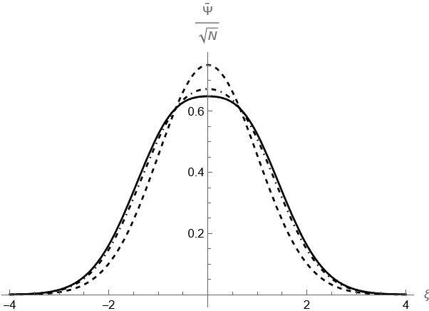
(a)

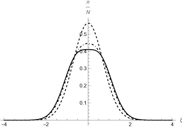
(b)

Figure 1: *

Fig.1.(a) Condensate wave-function vs $\xi$, (b) particle number density vs $\xi$ for an ideal Bose gas (dashed line), a dilute Bose gas with $N=1000$ particles (dot-dashed line) and $N=1300$ particles (full line).

The internal energy of the condensate is given by Eq.(62) which now reads:

$$\tilde{U}(N,\,\omega)=\,N\,[\frac{1}{2}+\,\frac{1}{{\sqrt{8\pi}}}\tilde{g}_{1}\,N\,]+O({(N\tilde{g}_{1})^{2}})$$ (80)

or in the dimension-full units

$$U(N,\,\omega)=\,N\,[\frac{D}{2}\hbar\omega+\,\frac{1}{2}\,{(\frac{{{m_{b}}\omega}}{{2\pi\hbar}})^{D/2}}\,g_{D}\,N\,\,]+O({(N\,g_{D})^{2}})),$$ (81)

with $D=1.$
We next calculate the mean-square radius of the condensate using Eq.(67)

$${\xi_{0}}=\,\sqrt{N{M_{0,0}}}\,\,[\,1\,-\,\frac{1}{{{M_{0,0}}}}\tilde{g}_{1}\,N\,\,\sum\limits_{n=1}^{\infty}{\,{T_{n}}}\,{M_{n,0}}+O({(N\tilde{g}_{1})^{2}})\,],$$ (82)

where

$${M_{n,0}}=\,\int{d\xi\,{\xi^{2}}\,}\frac{1}{{\sqrt{{2^{n}}\,n!\,\sqrt{\pi}}}}\,\,\exp(-\frac{1}{2}{\xi^{2}})\,{H_{n}}(\xi)\,{\chi_{0}}(\xi).\,$$

Using the recursion formulas for the Hermite polynomials [59, 58] we obtain

$${M_{n,0}}=\,(n+\frac{1}{2})\,{\delta_{n,0}}+\,\frac{1}{2}\,\sqrt{n(n-1)}\,{\delta_{n,2}}.$$ (83)

Inserting this back into Eq.(82) we get:

$${\xi_{0}}=\,\sqrt{\frac{N}{2}}\,(\,1\,+\,\frac{1}{{4\sqrt{2\pi}}}\tilde{g}_{1}\,N\,)+O({(N\tilde{g}_{1})^{2}}).$$ (84)

The inter-particle interactions increase the radius of the condensate.

7 The two-dimensional isotropic harmonic potential

We next consider the GP equation in two dimensions with the confining potential

$${V_{ext}}(x,y)=\frac{1}{2}{m_{b}}\,{\omega^{2}}\,({x^{2}}+{y^{2}}).$$ (85)

In this case the two-dimensional coupling constant is given by [53]

$${g_{2}}=g\,\sqrt{\frac{{{m_{b}}\,{\omega_{z}}}}{{2\,\pi\,\hbar}}},$$

and

$${{\tilde{g}}_{2}}=\frac{{4\,\pi\,a}}{{{l_{c}}}}\sqrt{\frac{{{\gamma_{z}}}}{{2\pi}}},$$ (86)

where,

$${l_{c}}=\,\,\sqrt{\frac{\hbar}{{{m_{b}}\,\omega}}};\,\,\,\,\,\,\,{\gamma_{z}}=\frac{{{\omega_{z}}}}{{{\omega}}}.$$

Because of the rotational symmetry of the problem we use plane polar coordinates $\vec{\xi}=\,(\xi,\varphi),$ where

$$\xi=\,\sqrt{\xi_{x}^{2}\,+\,\xi_{y}^{2}\,}\,\,\,\,\,\,\,\,\,\,\,\,0\leq\,\,\xi\,<\,\infty;\,\,\,\,\,\varphi={\tan^{-1}}(\frac{{{\xi_{y}}}}{{{\xi_{x}}}})\,\,\,\,\,\,\,\,\,\,\,\,0\,\,\leq\varphi<2\,\pi$$

Substituting Eq.(85) into Eq.(21), we obtain the eigenvalue problem for the two-dimensional isotropic harmonic oscillator with eigenvalues:

$${\lambda_{n,\,m}}\,=\,2n+|m|+1;\,\,\,\,\,\,\,\,\,\,n=0,\,1,\,2,\,...;\,\,\,\,\,\,\,\,\,\,m=0,\,\,\pm 1,\,\pm 2,\,...,$$ (87)

and eigenfunctions

$${\chi_{n,m}}(\xi,\,\varphi)\,=\,{A_{n,\,m}}\,{\xi^{|m|}}\,\,\exp(-\frac{1}{2}{\xi^{2}})\,L_{n}^{m}({\xi^{2}})\,\exp(i\,m\,\varphi),\,\,\,\,\,\,\,\,\,$$ (88)

where

$${A_{n,\,m}}\,=\,\sqrt{\frac{{n!}}{{\pi\,\Gamma(n+m+1)}}},\,\,\,\,$$ (89)

and $L_{n}^{m}(x)$ is the associated Laguerre polynomials of order $(n,m)$. The associated Laguerre polynomials $L_{n}^{k}(x)$, where $k$ can be a non-integer, is defined by [59, 58]:

$$L_{n}^{k}(x)\,=\,\frac{{{e^{x}}\,{x^{-k}}\,}}{{n!\,}}\,\frac{{{d^{n}}}}{{d{x^{n}}}}({e^{-x}}\,{x^{n+k}}),$$ (90)

and has the series representation:

$$L_{n}^{k}(x)\,=\,\sum\limits_{r\,=\,0}^{n}{{{(-1)}^{r}}}\,\frac{{\Gamma(n+k+1)}}{{r!\,(n-r)!\,\Gamma(k+r+1)}}\,{x^{r}},$$ (91)

and the generating function:

$$\frac{1}{{{{(1-t)}^{k+1}}}}\,\,\exp(-\,\,\frac{{x\,t}}{{1-t}})=\,\sum\limits_{n\,=\,0}^{\infty}{L_{n}^{k}(x)}\,{x^{n}}.$$ (92)

The ground-state eigenfunction,

$${\chi_{0,0}}(\xi,\varphi)\,=\frac{1}{{\sqrt{\pi}}}\,\,\exp(-\frac{1}{2}{\xi^{2}}),$$ (93)

is non-degenerate. We determine the coefficients ${b_{n,m}}\,$ by inserting Eq.(88) and Eq.(93) into Eq.(34) and evaluating the integral using the series representation Eq.(91). This gives

$${b_{n,m}}\,=\,\frac{1}{{\pi\,{2^{n+1}}}}\,{\delta_{m,0}};\,\,\,\,\,\,\,\,\,\,n=0,\,1,\,2,\,...;\,\,\,\,\,\,\,\,\,\,m=0,\,\,\pm 1,\,\pm 2,\,...\,.$$ (94)

From this expression we obtain:

$${T_{n,m}}\,=\,\frac{1}{{4\,\pi\,}}\frac{1}{{{2^{n}}\,n}}\,{\delta_{m,0}};\,\,\,\,\,\,\,\,\,\,n=\,1,\,2,\,...;\,\,\,\,\,\,\,\,\,\,m=0\,\pm 1,\,\pm 2,\,...,\,.$$ (95)

The condensate wave-function is then

$$\tilde{\psi}(\xi)\,=\,\sqrt{N}\{\,\,{\chi_{0,0}}(\xi)-\,\frac{1}{{4\,\pi}}\,\tilde{g}_{2}\,N\sum\limits_{n=1}^{\infty}{\frac{1}{{{2^{n}}\,n}}\,\,{\chi_{n,0}}(\xi)}\,\}+\,O({(N\tilde{g}_{2})^{2}})$$ (96)

We determine ${S^{(1)}}$ from Eq.(47):

$${S^{(1)}}=\,\sum\limits_{n=1}^{\infty}{\,\sum\limits_{m}{|{T_{n,m}}{|^{2}}}=\,\frac{1}{{16\,{\pi^{2}}}}\,\,\sum\limits_{n=1}^{\infty}{\,\frac{{{{(\frac{1}{4})}^{n}}\,}}{{{n^{2}}}}}}=\,\frac{1}{{16\,{\pi^{2}}}}\,{g_{2}}\,(\frac{1}{4}).$$

This gives

$${S^{(1)}}\,\simeq\,\frac{1}{{48\,{\pi^{2}}}}\,$$

For the experimental results in [61] with ${}^{87}Rb$, we have

$${m_{b}}\simeq 1.45\times{10^{-25}}Kg,\,\,\,\omega=2\pi\,\times\,20.6Hz,\,\,\,\,\omega_{z}=2\pi\,\times\,2KHz,\,\,\,\,a=\,5.3\times{10^{-9}}m\,,\,\,\,\,N=\,6.1\times{10^{4}}\,particles.$$

This gives:

$$\tilde{g}_{2}\,N\simeq\,0.11\,N\,\,\,\,\,\,and\,\,\,\,\,\,{({{\tilde{g}}_{2}}N)^{2}}\,{S^{(1)}}\,\simeq\,0.25\times{({10^{-2}}\,N)^{2}}$$

Thus for $N\geq{10^{2}}$ our interpretation is no longer valid because the perturbation theory breaks down for large numbers of particles. The chemical potential is now given by:

$$\tilde{\mu}\,=\,1+\,\frac{1}{{2\pi}}\tilde{g}_{2}\,N\,+O({(N\tilde{g}_{2})^{2}})$$ (97)

and in the dimension-full units is given by Eq.(78) with $D=2$. Again if we are interested in the second-order correction to the chemical potential we have

$${{\tilde{\mu}}_{2}}=\,-\,\frac{3}{{8\,{\pi^{2}}}}\,\ln(\frac{4}{3})\,\,{N^{2}}\,$$ (98)

The particle density is now given by:

$$n(\xi)\,=\,N\,[\chi_{0,0}^{2}(\xi)-\,\frac{1}{{2\pi}}\tilde{g}_{2}\,N\sum\limits_{n=1}^{\infty}{\frac{1}{{{2^{n}}n}}\,\,{\chi_{n,0}}(\xi)}\,{\chi_{0,0}}(\xi)]+\,O({(N\tilde{g}_{2})^{2}})$$ (99)

Figures 2.(a) and 2.(b) show respectively, $\tilde{\psi}(\xi)\,/\sqrt{N}$ and $n(\xi)/N$ for $N=30$ and $N=40$ particles and for $\tilde{g_{2}}$ calculated using the experimental data in [61]. Again the repulsive inter-particle interaction broadens the peak and shifts it down.

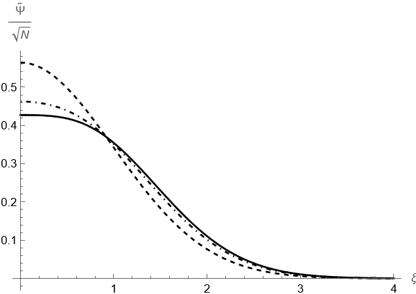
(a)

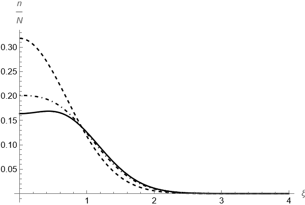
(b)

Figure 2: *

Fig.2.(a) Condensate wave-function vs $\xi$, (b) particle number density vs $\xi$ for an ideal Bose gas (dashed line), a dilute Bose gas with $N=30$ particles (dot-dashed line) and $N=40$ particles (full line).

The internal energy of the gas is obtained from Eq.(62)

$$\tilde{U}(N,\,\omega)=\,N\,[1+\,\frac{1}{{4\,\pi}}\tilde{g}_{2}\,N\,]+O({(N\tilde{g}_{2})^{2}})$$ (100)

and in the dimension-full units is given by Eq.(81) with $D=2$. To calculate the mean square radius of the condensate, we first calculate ${M_{m,n}}$ by substituting Eq.(88) into Eq.(66). We obtain

$${M_{(n,m),(0,0)}}=\,{\delta_{m,0}}\,I(n),$$

where

$$I(n)\,=\,2\,\int\limits_{0}^{\infty}{d\xi\,{\xi^{3}}}\,\exp(-{\xi^{2}})\,{L_{n}}({\xi^{2}}).$$

This integral can be easily evaluated using the generating function for the associated Laguerre polynomials (92) with $k=0.$ This gives:

$$I(0)=\,1,\,\,\,\,\,\,\,\,\,I(1)=\,-1,\,\,\,\,\,\,\,\,I(n)=0;\,\,\,\,\,\,n\geq 2$$

Hence the mean square radius of the condensate is:

$${\xi_{0}}=\,\sqrt{N}\,(\,1\,+\,\frac{1}{{8\,\pi}}\tilde{g}_{2}\,N\,)+O({(N\tilde{g}_{2})^{2}}).$$

8 The three-dimensional isotropic harmonic potential

We finally consider the GP equation in $D=3$ with the isotropic harmonic potential

$${V_{ext}}(x,y,\,z)=\frac{1}{2}{m_{b}}\,{\omega^{2}}\,({x^{2}}+{y^{2}}+{z^{2}}).$$ (101)

Since the potential ${V_{ext}}(x,y,\,z)$ has a spherical symmetry we use spherical coordinates $\vec{\xi}=\,(\xi,\,\theta,\,\varphi),$ where

$$\begin{gathered}\xi=\,\sqrt{\xi_{x}^{2}\,+\,\xi_{y}^{2}+\,\xi_{z}^{2}\,}\,\,\,\,\,\,\,\,\,\,\,\,0\leq\,\,\xi\,<\,\infty;\hfill\\ \theta={\cos^{-1}}(\frac{{{\xi_{x}}}}{\xi})\,\,\,\,\,\,\,\,\,\,\,\,0\,\,\leq\theta<\pi;\,\,\,\,\,\,\,\varphi={\tan^{-1}}(\frac{{{\xi_{y}}}}{{{\xi_{x}}}})\,\,\,\,\,\,\,\,\,\,\,\,0\,\,\leq\varphi<2\,\pi\hfill\\ \end{gathered}$$

Substituting Eq.(101) into Eq.(21) we obtain the eigenvalue problem for the isotropic three-dimensional oscillator with eigenfunctions

$$\begin{gathered}{\chi_{n,\,l,m}}(\xi,\,\theta,\,\,\varphi)\,=\,{A_{n,\,l}}\,{\xi^{l}}\,\,\exp(-\frac{1}{2}{\xi^{2}})\,L_{n}^{l+\frac{1}{2}}({\xi^{2}})\,Y_{l}^{m}\,(\theta,\,\,\varphi);\,\,\,\hfill\\ n=0,\,1,\,2,\,...;\,\,\,\,\,\,\,\,l=0,\,1,\,2,\,...;\,\,\,\,\,\,\,\,m=\,-l,\,-l+1,\,...,\,\,l,\,\hfill\\ \end{gathered}$$ (102)

where,

$${A_{n,\,l}}\,=\,\sqrt{\frac{{2(n!)}}{{\Gamma(n+l+\frac{3}{2})}}},\,\,\,\,$$ (103)

and $Y_{l}^{m}\,(\theta,\,\,\varphi)$ is the spherical harmonic function of order $(l,m)$. The eigenvalues depend only on $n$ and $l$ and are given by:

$${\lambda_{n,\,l}}\,=\,2n+l+\frac{3}{2};\,\,\,\,\,\,\,\,\,\,n=0,\,1,\,2,\,...;\,\,\,\,\,\,\,\,\,l=0,\,1,\,2,\,...\,.$$ (104)

The ground state eigenfunction,

$${\chi_{0,\,0,\,0}}(\xi,\,\theta,\,\varphi)\,={(\frac{1}{\pi})^{\frac{3}{4}}}\,\,\exp(-\frac{1}{2}{\xi^{2}}),$$ (105)

is non-degenerate. To determine ${b_{n,\,l,\,m}}$ we insert Eq.(102) and (105) into Eq.(34), this gives

$${b_{n,\,l,\,m}}\,=\,2\,{(\frac{1}{\pi})^{\frac{7}{4}}}\,{A_{n,\,l}}\,{\delta_{l,0}}\,{\delta_{m,0}}\,I(n),$$ (106)

where,

$$I(n)\,=\,\int\limits_{0}^{\infty}{d\xi\,{\xi^{2}}}\,\exp(-2\,{\xi^{2}})\,L_{n}^{\frac{1}{2}}({\xi^{2}}).$$

We may use the series expansion Eq.(91) with $k=1/2$ to evaluate the integral with the result,

$$I(n)\,\,=\,\frac{1}{{{2^{n+\frac{5}{2}}}\,n!}}\Gamma(n+\frac{3}{2}).$$

Substituting this back into Eq.(106), we obtain after some algebra

$${b_{n,\,l,\,m}}\,=\,\frac{1}{{{2^{2n+2}}\,n!}}\,{[\,\frac{{(\,2n+2\,)!}}{{{\pi^{3}}\,(\,n+1\,)}}\,]^{\frac{1}{2}}}\,\,{\delta_{l,0}}\,{\delta_{m,0}};\,\,\,\,\,\,\,\,\,\,\,\,\,\,\,n=0,\,1,\,2,\,...\,.\,$$ (107)

Then,

$${T_{n,\,l,\,m}}\,=\,\frac{1}{{{2^{2n+3}}\,n\,(n!)}}\,{[\,\frac{{(\,2n+2\,)!}}{{{\pi^{3}}\,(\,n+1\,)}}\,]^{\frac{1}{2}}}\,\,{\delta_{l,0}}\,{\delta_{m,0}};\,\,\,\,\,\,\,\,\,\,\,\,\,\,\,n=1,\,2,\,...\,.\,$$ (108)

The condensate wave-function now reads:

$$\tilde{\psi}(\xi)\,=\,\sqrt{N}\{\,\,{\chi_{0,\,0,\,0}}(\xi)-\,{(\frac{1}{{4\,\pi}})^{\frac{3}{2}}}\,\tilde{g}\,N\sum\limits_{n=1}^{\infty}{\,\frac{1}{{{2^{2n}}\,n\,(n!)}}\,{{[\,\frac{{(\,2n+2\,)!}}{{\,(\,n+1\,)}}\,]}^{\frac{1}{2}}}\,\,{\chi_{n,\,0,0}}(\xi)}\,\}+\,O({(N\tilde{g})^{2}})$$ (109)

We calculate ${S^{(1)}}$ using the inequality:

$$(2n+1)(2n)!\leq\,{2^{2n+1}}\,n\,{(n!)^{2}},$$ (110)

leading to

$${S^{(1)}}=\,\sum\limits_{n=1}^{\infty}{\,\sum\limits_{l,\,m}{|{T_{n,\,l,\,m}}{|^{2}}}}\leq\,\frac{1}{{16\,{\pi^{3}}}}\,\sum\limits_{n=1}^{\infty}{\,\frac{{{{(\frac{1}{4})}^{n}}\,}}{n}}=\,\frac{1}{{16\,{\pi^{3}}}}\,\ln(\frac{4}{3}).$$

For the experimental results in [62] using ${}^{87}Rb$ atoms, we have

$${m_{b}}\sim\,1.45\times{10^{-25}}Kg,\,\,\,{\omega}\sim\,2\pi\times 77.5\,\,Hz,\,\,\,\,a\approx\,5.8\times{10^{-9}}m\,,\,\,\,\,N\sim\,1.2\times{10^{5}}\,particles$$

This gives:

$$\tilde{g}\,N\simeq\,0.61\times{10^{-1}}\,N\,\,\,\,\,\,$$

The fraction of the Bose particles tunneling to the excited states is now

$${(\tilde{g}\,N)^{2}}\,{S^{(1)}}\sim\,0.32\,\times(10^{-2}N)^{2}.$$

For $N\geq{10^{2}}$ our interpretation is no longer valid, this is because the actual expansion coefficient $\tilde{g}\,N$ is very large and the perturbation theory breaks down. The chemical potential is given by

$$\tilde{\mu}\,=\,\frac{3}{2}+\,{(\frac{1}{{2\pi}})^{\frac{3}{2}}}\tilde{g}\,N\,+O({(N\tilde{g})^{2}}),$$ (111)

and in the dimension-full units by Eq.(78) with $D=3$. The second order correction is given by Eq.(58), which now reads:

$${{\tilde{\mu}}_{2}}\simeq\,-\,\frac{{3\,{N^{2}}}}{{16\,{\pi^{3}}}}\,\sum\limits_{n=1}^{\infty}{\,\frac{{(2n+1)\,(\,2n\,)!}}{{{2^{4n}}\,n\,{{(n!)}^{2}}}}\,.\,}\,$$ (112)

Instead of summing this series we will obtain an upper bound on its sum using the inequality Eq.(110). This gives

$${{\tilde{\mu}}_{2}}\simeq\,-\,\frac{{3\,{N^{2}}}}{{8\,{\pi^{3}}}}\,\sum\limits_{n=1}^{\infty}{\,{{(\frac{1}{4})}^{n}}\,=\,}\,-\,\frac{{{N^{2}}}}{{8\,{\pi^{3}}}}.$$ (113)

The particle density now reads

$$n(\xi)\,=\,N\{\,\,\chi_{0,\,0,\,0}^{2}(\xi)-\,{(\frac{1}{{2\,\pi}})^{\frac{3}{2}}}\,\tilde{g}\,N\sum\limits_{n=1}^{\infty}{\,\frac{{\sqrt{(\,2n+1\,)!}}}{{{2^{2n}}\,n\,\,(n!)}}\,\,{\chi_{n,\,0,0}}(\xi)}\,{\chi_{0,\,0,\,0}}(\xi)\}+\,O({(N\tilde{g})^{2}}).$$ (114)

Figures 3.(a) and 3.(b) show respectively, $\tilde{\psi}(\xi)\,/\sqrt{N}$ and $n(\xi)/N$ for $N=30$ and $N=40$ particles and for $\tilde{g}$ calculated using the experimental data in [62]. Again the repulsive inter-particle interaction broadens the peak and shifts it down.

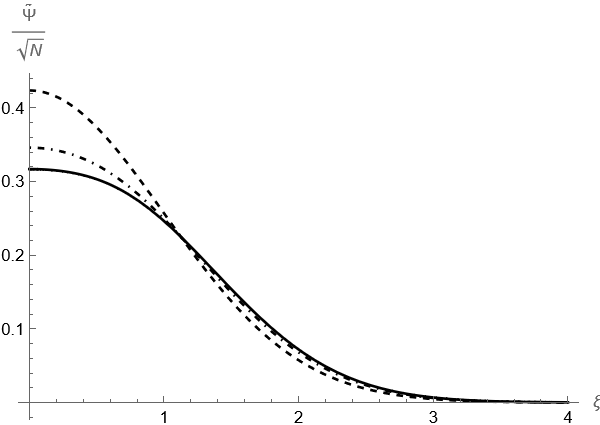
(a)

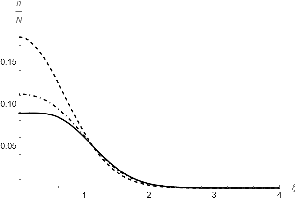
(b)

Figure 3: *

Fig.3.(a) Condensate wave-function vs $\xi$, (b) particle number density vs $\xi$ for an ideal Bose gas (dashed line), a dilute Bose gas with $N=30$ particles (dot-dashed line) and $N=40$ particles (full line).

We calculate the internal energy of the gas using Eq.(62)

$$\tilde{U}(N,\,\omega)=\,N\,[\frac{3}{2}+\,\frac{1}{2}\,{(\frac{1}{{2\,\pi}})^{\frac{3}{2}}}\tilde{g}\,N\,]+O({(N\tilde{g})^{2}}),$$ (115)

And in the dimension-full units is given by Eq.(81) with $D=3$. Finally we calculate the mean-square radius of the condensate by inserting Eqs.(102) and (105) into Eq.(66)

$${M_{(n,\,l,\,m),\,(0,\,0,\,0)}}=\,2\,{(\frac{1}{\pi})^{\frac{1}{4}}}\,{[\,\frac{{2(\,n\,!)}}{{\,\Gamma(\,n+\frac{3}{2}\,)}}\,]^{\frac{1}{2}}}I(n)\,{\delta_{l,0}}\,{\delta_{m,0}}\,,$$ (116)

where,

$$I(n)\,=\,\frac{1}{2}\,\,\int\limits_{0}^{\infty}{dx\,{x^{\frac{3}{2}}}}\,{\operatorname{e}^{-x}}\,L_{n}^{\frac{1}{2}}(x).$$

Using the generating function Eq.(92) with $k=\frac{1}{2}$ we obtain:

$$I(0)=\,\frac{1}{2}\,\Gamma(\frac{5}{2}),\,\,\,\,\,\,\,\,\,I(1)=\,-\frac{1}{2}\,\Gamma(\frac{5}{2}),\,\,\,\,\,\,\,\,I(n)=0;\,\,\,\,\,\,n\geq 2.$$

This gives

$${\xi_{0}}=\,\frac{3}{2}\sqrt{\frac{N}{\pi}}\,(\,1\,+\,\frac{{\sqrt{2}}}{{16\,\pi}}\tilde{g}\,N\,)+O({(N\tilde{g})^{2}}).$$ (117)

9 Conclusion

We have studied the perturbative solution of the Gross-Pitaevskii(GP) equation in the $D$-dimensional space $R^{D}$ with a general confining potential, $V_{ext}(\vec{r})$. The solution describes the condensate wave-function of a gas of $N$ Bose particles under the influence of the external potential and the two-body inter-particle interactions ${g_{D}}\,{\delta^{D}}(\vec{r}-\vec{r}^{\prime})$.
We obtained the condensate wave-function corrected to first order in, $g_{D}\,N$, which is the actual expansion parameter. We showed that if the number $N$ of the Bose particles exceeds a certain number, which depends on $g_{D}$ and the dimension $D$, of the condensate then the perturbation theory breaks down. We calculated the physical parameters; the particle density, the chemical potential, the internal energy and the mean-square radius of the condensate to first order in, $g_{D}\,N$.
We applied the method to the GP equation in $D=1$ with a harmonic potential. The solution represents a cigar-shaped Bose condensate using the experimental data [60]. We showed that the perturbative solution breaks down if $N$ exceeds $1300$ particles. We also studied the $D=2$ and $D=3$ with a rotationally symmetric and spherically symmetric harmonic potentials respectively. In both cases the maximum number of particles that can be described by the perturbative solution does not exceed $40$ particles for the data in references [61, 62].
This is a major disadvantage of the perturbative approach since it cannot be used to compare with the experimental results which use a number of particles in the range $10^{6}\sim 10^{7}$. However, it sheds light on the nature of the solution and allows us to compute important physical parameters of the system as we have seen.
It is very interesting to apply the perturbative method to obtain solutions of the GP equation with more realistic two-body interactions. Also to extend the method to the investigation of the time-dependent GP equation as well as to the study of the excited states of the Bose condensate.

References

• Bradley et al. [1995] Bradley CC, Sackett CA, Tollett JJ, Hulet RG. Evidence of bose-einstein condensation in an atomic gas with attractive interactions. Physical Review Letters 1995;75:1687–90. doi:10.1103/PhysRevLett.75.1687.
• Anderson et al. [1995] Anderson MH, Ensher JR, Matthews MR, Wieman CE, Cornell EA. Observation of bose-einstein condensation in a dilute atomic vapor. Science 1995;269:198–201. doi:10.1126/science.269.5221.198.
• Davis et al. [1995] Davis KB, Mewes MO, Andrews MR, van Druten NJ, Durfee DS, Kurn DM, et al. Bose-einstein condensation in a gas of sodium atoms. Physical Review Letters 1995;75:3969–73. doi:10.1103/PhysRevLett.75.3969.
• Gross [1961] Gross EP. Structure of a quantized vortex in boson systems. Il Nuovo Cimento 1961;20:454–77. doi:10.1007/BF02731494.
• Pitaevskii [1961] Pitaevskii LP. Vortex lines in an imperfect bose gas. Sov Phys JETP 1961;13(2):451–4.
• Parkins and Walls [1998] Parkins A, Walls D. The physics of trapped dilute-gas bose–einstein condensates. Physics Reports 1998;303:1–80. doi:10.1016/S0370-1573(98)00014-3.
• Dalfovo et al. [1999] Dalfovo F, Giorgini S, Pitaevskii LP, Stringari S. Theory of bose-einstein condensation in trapped gases. Reviews of Modern Physics 1999;71:463–512. doi:10.1103/RevModPhys.71.463.
• Leggett [2001] Leggett AJ. Bose-einstein condensation in the alkali gases: Some fundamental concepts. Reviews of Modern Physics 2001;73:307–56. doi:10.1103/RevModPhys.73.307.
• Morsch and Oberthaler [2006] Morsch O, Oberthaler M. Dynamics of bose-einstein condensates in optical lattices. Reviews of Modern Physics 2006;78:179–215. doi:10.1103/RevModPhys.78.179.
• Yukalov [2011] Yukalov VI. Basics of bose-einstein condensation. Physics of Particles and Nuclei 2011;42:460–513. doi:10.1134/S1063779611030063.
• Pethick and Smith [2002] Pethick CJ, Smith H. Bose-Einstein Condensation in Dilute Gases. 2002.
• Pitaevskii and Stringari [2003] Pitaevskii LP, Stringari S. Bose-Einstein Condensation. Clarendon; 2003.
• Liu and Kengne [2019] Liu WM, Kengne EK. Schrödinger Equations in Nonlinear Systems. First ed.; Springer; 2019.
• Efremidis et al. [2009] Efremidis NK, Siviloglou GA, Christodoulides DN. Exact x-wave solutions of the hyperbolic nonlinear schrödinger equation with a supporting potential. Physics Letters A 2009;373:4073–6. doi:10.1016/j.physleta.2009.09.008.
• Barashenkov et al. [2015] Barashenkov IV, Zezyulin DA, Konotop VV. Exactly solvable wadati potentials in the pt-symmetric gross-pitaevskii equation 2015;doi:10.1007/978-3-319-31356-6_9.
• Kivshar and Agrawal [2003] Kivshar YS, Agrawal GP. Optical Solitons From Fibers to Photonic Crystals. Academic Press; 2003.
• Moffat [2006] Moffat JW. Spectrum of cosmic microwave fluctuations and the formation of galaxies in a modified gravity theory 2006;doi:https://doi.org/10.48550/arXiv.astro-ph/0602607.
• Cunillera and Germani [2018] Cunillera F, Germani C. The gross–pitaevskii equations of a static and spherically symmetric condensate of gravitons. Classical and Quantum Gravity 2018;35:105006. doi:10.1088/1361-6382/aab97b.
• Yang et al. [2019] Yang Y, Wang Y, Zhao L, Song D, Zhou Q, Wang W. Sonic black hole horizon formation for bose-einstein condensates with higher-order nonlinear effects. AIP Advances 2019;9:115203. doi:10.1063/1.5124934.
• Jacquet et al. [2020] Jacquet MJ, Boulier T, Claude F, Maître A, Cancellieri E, Adrados C, et al. Polariton fluids for analogue gravity physics. Philosophical Transactions of the Royal Society A: Mathematical, Physical and Engineering Sciences 2020;378:20190225. doi:10.1098/rsta.2019.0225.
• Anglin and Ketterle [2002] Anglin JR, Ketterle W. Bose–einstein condensation of atomic gases. Nature 2002;416:211–8. doi:10.1038/416211a.
• Burchianti et al. [2017] Burchianti A, Fort C, Modugno M. Josephson plasma oscillations and the gross-pitaevskii equation: Bogoliubov approach versus two-mode model. Physical Review A 2017;95:023627. doi:10.1103/PhysRevA.95.023627.
• Han [2017] Han JH. Skyrmions in Condensed Matter. Springer International Publishing AG; 2017.
• Minguzzi [2004] Minguzzi A. Numerical methods for atomic quantum gases with applications to bose–einstein condensates and to ultracold fermions. Physics Reports 2004;395:223–355. doi:10.1016/j.physrep.2004.02.001.
• Bao and Tang [2003] Bao W, Tang W. Ground-state solution of bose–einstein condensate by directly minimizing the energy functional. Journal of Computational Physics 2003;187:230–54. doi:10.1016/S0021-9991(03)00097-4.
• Edwards and Burnett [1995] Edwards M, Burnett K. Numerical solution of the nonlinear schrödinger equation for small samples of trapped neutral atoms. Physical Review A 1995;51:1382–6. doi:10.1103/PhysRevA.51.1382.
• Adhikari [2000a] Adhikari SK. Numerical study of the spherically symmetric gross-pitaevskii equation in two space dimensions. Physical Review E 2000a;62:2937–44. doi:10.1103/PhysRevE.62.2937.
• Adhikari [2000b] Adhikari SK. Numerical solution of the two-dimensional gross–pitaevskii equation for trapped interacting atoms. Physics Letters A 2000b;265:91–6. doi:10.1016/S0375-9601(99)00878-6.
• Chiofalo et al. [2000] Chiofalo ML, Succi S, Tosi MP. Ground state of trapped interacting bose-einstein condensates by an explicit imaginary-time algorithm. Physical Review E 2000;62:7438–44. doi:10.1103/PhysRevE.62.7438.
• Cerimele et al. [2000] Cerimele MM, Chiofalo ML, Pistella F, Succi S, Tosi MP. Numerical solution of the gross-pitaevskii equation using an explicit finite-difference scheme: An application to trapped bose-einstein condensates. Physical Review E 2000;62:1382–9. doi:10.1103/PhysRevE.62.1382.
• Adhikari [2001] Adhikari SK. Numerical study of the coupled time-dependent gross-pitaevskii equation: Application to bose-einstein condensation. Physical Review E 2001;63:056704. doi:10.1103/PhysRevE.63.056704.
• Muruganandam and Adhikari [2003] Muruganandam P, Adhikari SK. Bose–einstein condensation dynamics in three dimensions by the pseudospectral and finite-difference methods. Journal of Physics B: Atomic, Molecular and Optical Physics 2003;36:2501–13. doi:10.1088/0953-4075/36/12/310.
• Bao et al. [2003] Bao W, Jaksch D, Markowich PA. Numerical solution of the gross–pitaevskii equation for bose–einstein condensation. Journal of Computational Physics 2003;187:318–42. doi:10.1016/S0021-9991(03)00102-5.
• Antoine et al. [2013] Antoine X, Bao W, Besse C. Computational methods for the dynamics of the nonlinear schrödinger/gross–pitaevskii equations. Computer Physics Communications 2013;184:2621–33. doi:10.1016/j.cpc.2013.07.012.
• Carr et al. [2000a] Carr LD, Clark CW, Reinhardt WP. Stationary solutions of the one-dimensional nonlinear schrödinger equation. i. case of repulsive nonlinearity. Physical Review A 2000a;62:063610. doi:10.1103/PhysRevA.62.063610.
• Bronski et al. [2001a] Bronski JC, Carr LD, Deconinck B, Kutz JN, Promislow K. Stability of repulsive bose-einstein condensates in a periodic potential. Physical Review E 2001a;63:036612. doi:10.1103/PhysRevE.63.036612.
• Carr et al. [2000b] Carr LD, Clark CW, Reinhardt WP. Stationary solutions of the one-dimensional nonlinear schrödinger equation. ii. case of attractive nonlinearity. Physical Review A 2000b;62:063611. doi:10.1103/PhysRevA.62.063611.
• Bronski et al. [2001b] Bronski JC, Carr LD, Carretero-González R, Deconinck B, Kutz JN, Promislow K. Stability of attractive bose-einstein condensates in a periodic potential. Physical Review E 2001b;64:056615. doi:10.1103/PhysRevE.64.056615.
• Hua-Mei [2005] Hua-Mei L. New exact solutions of nonlinear gross–pitaevskii equation with weak bias magnetic and time-dependent laser fields. Chinese Physics 2005;14:251–6. doi:10.1088/1009-1963/14/2/006.
• Belmonte-Beitia et al. [2008] Belmonte-Beitia J, Pérez-García VM, Vekslerchik V, Konotop VV. Localized nonlinear waves in systems with time- and space-modulated nonlinearities. Physical Review Letters 2008;100:164102. doi:10.1103/PhysRevLett.100.164102.
• Belmonte-Beitia et al. [2009] Belmonte-Beitia J, Konotop VV, Pérez-García VM, Vekslerchik VE. Localized and periodic exact solutions to the nonlinear schrödinger equation with spatially modulated parameters: Linear and nonlinear lattices. Chaos, Solitons and Fractals 2009;41:1158–66. doi:10.1016/j.chaos.2008.04.057.
• Yu [2013] Yu F. Three-dimensional exact solutions of gross–pitaevskii equation with variable coefficients. Applied Mathematics and Computation 2013;219:5779–86. doi:10.1016/j.amc.2012.11.089.
• Malomed and Stepanyants [2010] Malomed BA, Stepanyants YA. The inverse problem for the gross–pitaevskii equation. Chaos: An Interdisciplinary Journal of Nonlinear Science 2010;20:013130. doi:10.1063/1.3367776.
• Neirameh [2016] Neirameh A. Exact analytical solutions for 3d- gross–pitaevskii equation with periodic potential by using the kudryashov method. Journal of the Egyptian Mathematical Society 2016;24:49–53. doi:10.1016/j.joems.2014.11.004.
• Liu et al. [2021] Liu YY, Li WD, Dai WS. Exactly solvable gross–pitaevskii type equations. Journal of Physics Communications 2021;5:1–11. doi:10.1088/2399-6528/abda12.
• Baym and Pethick [1996] Baym G, Pethick CJ. Ground-state properties of magnetically trapped bose-condensed rubidium gas. Physical Review Letters 1996;76:6–9. doi:10.1103/PhysRevLett.76.6.
• Fetter [1997] Fetter AL. Variational study of dilute bose condensate in a harmonic trap. Journal of Low Temperature Physics 1997;106:643–52. doi:10.1007/BF02395929.
• Pérez-García et al. [1997] Pérez-García VM, Michinel H, Cirac JI, Lewenstein M, Zoller P. Dynamics of bose-einstein condensates: Variational solutions of the gross-pitaevskii equations. Physical Review A 1997;56:1424–32. doi:10.1103/PhysRevA.56.1424.
• Kivshar et al. [2001] Kivshar YS, Alexander TJ, Turitsyn SK. Nonlinear modes of a macroscopic quantum oscillator. Physics Letters A 2001;278:225–30. doi:10.1016/S0375-9601(00)00774-X.
• Trallero-Giner et al. [2008] Trallero-Giner C, Drake-Perez JC, López-Richard V, Birman JL. Formal analytical solutions for the gross–pitaevskii equation. Physica D: Nonlinear Phenomena 2008;237:2342–52. doi:10.1016/j.physd.2008.02.017.
• Shi et al. [2012] Shi YR, Wang GH, Liu CB, Zhou ZG, Yang HJ. Analytical solutions to the time-independent gross-pitaevskii equation with a harmonic trap. Chinese Physics Letters 2012;29:110302. doi:10.1088/0256-307X/29/11/110302.
• Jia-Ren et al. [2002] Jia-Ren Y, Jing L, Sheng-Mei A, Dong-Bo C. Bose-einstein condensation in a spherical symmetric harmonic trap. Chinese Physics Letters 2002;19:1245–7. doi:10.1088/0256-307X/19/9/308.
• Dion and Cancès [2007] Dion CM, Cancès E. Ground state of the time-independent gross–pitaevskii equation. Computer Physics Communications 2007;177:787–98. doi:10.1016/j.cpc.2007.04.007.
• Myškis [1979] Myškis AD. ADVANCED MATHEMATICS for ENGINEERS: Special Courses. Mir publishers; 1979.
• Titchmarsh [1962] Titchmarsh EC. Eigenfunction Expansions associated with Second-order Differential Equations; vol. I. Second edition ed.; Oxford University Press; 1962.
• Titchmarsh [1958] Titchmarsh EC. Eigenfunction Expansions associated with Second-order Differential Equations; vol. II. Oxford University Press; 1958.
• Moiseiwitsch [1977] Moiseiwitsch BL. Integral Equations. 1977.
• Bell [2004] Bell WW. Special Functions for Scientists and Engineers. Dover Publications; 2004.
• Lebedev [1972] Lebedev NN. Special Functions and Their Applications. Dover Publications; 1972.
• Denschlag et al. [2002] Denschlag JH, Simsarian JE, Häffner H, McKenzie C, Browaeys A, Cho D, et al. A bose-einstein condensate in an optical lattice. Journal of Physics B: Atomic, Molecular and Optical Physics 2002;35:307. doi:10.1088/0953-4075/35/14/307.
• Yefsah et al. [2011] Yefsah T, Desbuquois R, Chomaz L, Günter KJ, Dalibard J. Exploring the thermodynamics of a two-dimensional bose gas. Physical Review Letters 2011;107:130401. doi:10.1103/PhysRevLett.107.130401.
• Li et al. [2019] Li RZ, Gao TY, Zhang DF, Peng SG, Kong LR, Shen X, et al. Expansion dynamics of a spherical bose–einstein condensate*. Chinese Physics B 2019;28:106701. doi:10.1088/1674-1056/ab4177.