Geometric Batch Optimization for the Packing Equal Circles in a Circle Problem on Large Scale

Abstract

The problem of packing equal circles in a circle is a classic and famous packing problem, which is well-studied in academia and has a variety of applications in industry. This problem is computationally challenging, and researchers mainly focus on small-scale instances with the number of circular items $n$ less than 320 in the literature. In this work, we aim to solve this problem on large scale. Specifically, we propose a novel geometric batch optimization method that not only can significantly speed up the convergence process of continuous optimization but also reduce the memory requirement during the program’s runtime. Then we propose a heuristic search method, called solution-space exploring and descent, that can discover a feasible solution efficiently on large scale. Besides, we propose an adaptive neighbor object maintenance method to maintain the neighbor structure applied in the continuous optimization process. In this way, we can find high-quality solutions on large scale instances within reasonable computational times. Extensive experiments on the benchmark instances sampled from $n=$ 300 to 1,000 show that our proposed algorithm outperforms the state-of-the-art algorithms and performs excellently on large scale instances. In particular, our algorithm found 10 improved solutions out of the 21 well-studied moderate scale instances and 95 improved solutions out of the 101 sampled large scale instances. Furthermore, our geometric batch optimization, heuristic search, and adaptive maintenance methods are general and can be adapted to other packing and continuous optimization problems.

1 Introduction

The packing problems are a typical class of optimization problems that aim to pack a set of geometric objects into one or multiple containers, and the goal is to either find a configuration that is as dense as possible or find a solution with as few containers (bins) as possible. The packing problems have a rich research history, with numerous variants being proposed, and a number of studies and methods being published for solving these problems, such as circle packing (Huang and Ye, 2011; He et al., 2018; Lai et al., 2022), sphere packing (Hartman et al., 2019; Hifi and Yousef, 2019), square packing (Leung et al., 1990; Fekete and Hoffmann, 2017), cube packing (Miyazawa and Wakabayashi, 2003; Epstein and van Stee, 2005), irregular packing (Leao et al., 2020; Zhao et al., 2020; Rao et al., 2021) and bin packing (Baldi et al., 2019; Zhao et al., 2021; He et al., 2021), etc.

As one of the most popular packing problems, the Circle Packing Problem (CPP) has been widely studied in mathematics and computer science fields. Given $n$ circular items with fixed radii, the CPP aims to pack all the $n$ items into a container so that all the items are totally contained in the container without overlapping with each other, and the container size is minimized. Specifically, if the container is square, then the goal is to minimize the side length of the square container; and if the container is circular, then the goal is to minimize the radius of the circular container. There are also other CPP variants (López and Beasley, 2011) based on different geometric containers.

CPP has a lot of industrial applications, such as facility layout, cylinder packing, circular cutting, container loading, dashboard layout (Castillo et al., 2008), structure design (Yanchevskyi et al., 2020) and satellite packaging (Wang et al., 2019). Furthermore, the solution of CPP can be applied to data visualization and data analysis (Wang et al., 2006; Murakami et al., 2015; Görtler et al., 2017). On the other hand, CPP is proved to be NP-hard (Demaine et al., 2010), therefore solving this problem is computationally challenging. In particular, there is a special variant of CPP, called Packing Equal Circles in a Circle (PECC), which aims to pack $n$ unit circles into a circular container with the smallest possible radius. Since PECC is representative and simple in form, it has become the most famous and well-studied problem in the CPP family, to which numerous efforts have been devoted.

Since the CPP is NP-hard, the computational resource and difficulty for obtaining a high-quality configuration grow exponentially with the number of circular items to be packed, and solving the large scale instances of CPP is extremely difficult. Therefore, most works for CPP focus on solving instances on small or moderate scale, and only a few efforts are devoted to solving large scale instances. In this work, we address the PECC variant of CPP. Based on the classic elastic model (Huang and Xu, 1999; He et al., 2018) (also known as Quasi-Physical Quasi-Human model, QPQH), we propose a Geometric Batch Optimization (GBO) method that can construct a feasible solution or an infeasible solution with the overlaps being as few as possible on large scale instances. Different from existing methods, GBO divides the packing circles into several geometric batches. Then, in the non-convex continuous optimization process, GBO alternately updates each batch of packing circles instead of updating all the circles. In this way, GBO reduce the time and space complexity, which can not only significantly speed up the convergence process of the non-convex continuous optimization but also reduce the resident memory requirement during the program’s runtime.

In addition, we propose an Adaptive Neighbor object Maintenance (ANM) method to maintain the neighbor structure (He et al., 2018) for the continuous optimization process. ANM uses two variables “$counter$” and “$deferring\leavevmode\nobreak\ length$” to accomplish the adaptive feature. When the layout is changing significantly, ANM maintains the neighbors in each iteration, otherwise, ANM defers the maintaining process. Our ANM method can handle some issues and disadvantages of the existing methods (He et al., 2018; Lai et al., 2022) and it can adopt to solve dynamic packing problems or online packing problems.

Finally, we propose an advanced local search heuristic, called Solution-space Exploring and Descent (SED), based on the GBO module to solve the PECC problem. SED perturbs the current solution to obtain several perturbed candidate solutions. Then, SED employs the GBO module to minimize the overlap of each candidate solution and takes a solution with minimal overlap among the candidate solutions to replace the current solution. The algorithm could efficiently find a high-quality solution by iteratively executing the SED heuristic procedure.

The experimental results show that our GBO method dramatically accelerates the convergence speed of the non-convex continuous process and reduces memory consumption. Specifically, GBO reduces the convergence time by 32.74% to 54.11% and the runtime resident memory by 36.00% to 39.04% compared with the typical non-batch method on large scale instances for $n=$ 500 to 1,000. By combining the GBO module into SED to solve 101 large scale instances, including 51 regular numbers and 50 irregular numbers selected from 500 $\leq n\leq$ 1,000, our method improves the best-known solution for 95 instances reported in Packomania website (Specht, 2022). Besides, our method is also efficient on moderate scale instances, because it improves the best-known solution for 10 instances among the 21 well-studied moderate scale instances, 300 $\leq n\leq$ 320, which were solved by the state-of-the-art algorithm called IDTS (Lai et al., 2022). Through these experiments, GBO shows clear advantages over existing methods for solving large scale packing instances and SED is an efficient heuristic.

The main contributions of this work are summarized as follows:

• We propose a novel method called Geometric Batch Optimization (GBO), which divides the circles into several geometric batches and speeds up the computation significantly.

• We propose an Adaptive Neighbor object Maintenance (ANM) method of the neighbor structure for solving the PECC problem.

• We propose an efficient Solution-space Exploring and Descent (SED) heuristic with the GBO as a sub-module for solving the PECC problem.

• Extensive experiments on large scale instances sampled from $n=500$ to 1,000, as well as moderate instances for $n=300$ to 320, demonstrate the excellent performance and efficiency of our proposed algorithm, gaining new best solutions on many instances.

The rest of this paper is organized as follows. Section 2 presents the related works of the CPP and PECC problem, including the landmark models, the landmark heuristics, and the recent works for solving the CPP and PECC problems. Section 3 introduces the mathematical formula of the PECC problem and the famous and powerful elastic model (QPQH) that is adopted in this work. Section 4 presents the continuous optimization methods, including our proposed GBO method, the container adjusting method, and our ANM method, which are the essential modules adopted in our final heuristic. Section 5 presents the discrete optimization method (i.e., SED heuristic), which is our final algorithm for solving the PECC problem. Section 6 presents the experimental results of our proposed algorithm compared with the best-known results and the state-of-the-art algorithm and parameter study. The conclusion is drawn in the end.

2 Related Work

In this section, We briefly review the works on CPP, including some typical works, landmark models, and landmark heuristics, then we review the recent works on the PECC problem.

Early works for solving CPP focus on solving the PECC variant using mathematical analysis with the goal of finding and proving an optimal solution for small scale instances. Starting from 1967, Kravitz (1967) first provided the solutions for $2\leq n\leq 19$. Subsequently, Graham and Peck (1968) proved the optimality for $2\leq n\leq 7$. In 1969, Pirl (1969) further proved the optimality of the solutions for $2\leq n\leq 10$ and also provided solutions for $11\leq n\leq 19$. In 1971, Goldberg (1971) improved the solutions for $n=14,16,17$ and further provided the solution for $n=20$. In 1975, Reis (1975) provided the solutions for $21\leq n\leq 25$. Melissen (1994) proved the optimality for $n=11$ and Fodor (1999, 2000, 2003) proved the optimality for $n=12,13,19$. To summarize, the optimality for $2\leq n\leq 13$ and $n=19$ has been proven. For larger instances, it is hard to find and prove the optimality of a solution by exploiting mathematical analysis. Thereafter, most efforts are devoted to designing efficient heuristic algorithms.

The discrete optimization model is one of the popular techniques for solving CPP, of which the idea is to pack each circle one by one into the container. If there exists a placement order by which all the circles can be packed into the container, then the solution is found. A circle placement heuristic is essential to this model, because it directly impacts the placement strategies and the performance. Huang et al. (2003) and Huang et al. (2006) propose a classic circle placement heuristic, called Corner-Occupying Placement (COP), and a metric function for placement action, named Maximal Hole Degree (MHD), on the unequal circle packing problem. COP requests each current packing circle contact with two packed circles or the boundary of the container and does not overlap with other circles, and the MHD function can measure the quality of the candidate action of the circle placement. There are several follow-up works based on COP heuristic and MHD function to either solve other variants or improve the algorithm efficiency: Huang et al. (2005) adopt this heuristic for packing circles in a rectangular container; Lü and Huang (2008) apply a Pruned–Enriched-Rosenbluth Method (PERM) to improve the performance on the unequal circle packing problem; Akeb et al. (2009, 2010) further employ the beam search and adaptive beam search algorithms to improve the performance on unequal circle packing problems, and Chen et al. (2018) present a greedy heuristic algorithm for solving the PECC problem. There also exist other circle placement heuristics for solving the packing problems, such as Bottom-Left-Fill (Martello et al., 2003; Burke et al., 2006) and Best Local Position (Hifi and M’Hallah, 2004, 2007).

However, due to the characteristic of the discrete optimization model, it takes massive computational time to obtain a dense solution on moderate or large scale instances. Therefore, most researchers prefer to adopt the non-convex continuous optimization model to solve moderate scale CPP. Inspired by the physical model, some quasi-physical models have been proposed for solving CPP. Graham et al. (1998) design a molecular repulsion model and a Billiards model for solving the PECC problem, and these models are also applied to solve other packing variants (Nurmela and Östergård, 1997). Some efforts are devoted to designing an efficient local search heuristic based on the elastic model, termed Quasi-Physical Quasi-Human (QPQH), proposed by Huang and Xu (1999) for solving CPP and its variants: Huang and Ye (2011) propose a basin hopping heuristic of attractive force model to solve the PECC problem; He et al. (2018) propose a shrinking basin-hopping heuristic to solve the PECC problem; Lai et al. (2022) adopt the iterated dynamic thresholding search to solve the PECC problem; He et al. (2013) employ the elastic model to solve circle packing problem with equilibrium constraints and Liu et al. (2016) employ the elastic model to solve the weighted circle packing problem.

There also exist other methods and heuristics for solving CPP, such as monotonic basin hopping and population basin hopping heuristics (Addis et al., 2008; Grosso et al., 2010), simulated annealing approach (Hifi et al., 2004), genetic algorithm-based approach (Hifi and M’Hallah, 2004), tabu search approach (Carrabs et al., 2014), non-linear programming based approach (Mladenović et al., 2005; Birgin and Sobral, 2008; Stoyan and Yaskov, 2014), mixed-strategy (Stoyan et al., 2020), etc.

The well-known Packomania website (Specht, 2022) maintained by Specht presents many circle packing problems and records their best-known solutions. According to the number of solutions, the scale of solutions, and the recently updated history, we observe that the PECC problem and the problem of circle packing in a rectangle are popular and well-studied, and the recent algorithms for solving the two problems are similar to the methods mentioned above, suggesting that these methods and algorithms have good universality and generality on different circle packing problems and their variants.

From the recently updated history on PECC with $n\geq 100$ at Packomania, we observe the current best-known records as follows: Huang and Ye (2011) hold several best-known solutions for $100\leq n\leq 200$; Cantrell holds several best-known solutions for $110\leq n\leq 1039$ with unpublished methods; Donovan holds three best-known solutions for $n=85,109$ and $121$ with unpublished methods; Lai et al. (2022) hold a number of best-known solutions for $126\leq n\leq 319$, Stoyan et al. (2020) hold 16 best-known solutions for $1077\leq n\leq 5000$, and the remaining best-known solutions are held by Specht with unpublished methods. In summary, the elastic model (QPQH) based methods (Huang and Ye, 2011; Lai et al., 2022) and mixed-strategy method (Stoyan et al., 2020) can be regarded as the state-of-the-art algorithms for solving the PECC problem.

3 Preliminaries

3.1 Problem Formulation

The PECC problem aims to pack $n$ unit circles $\{c_{1},c_{2},...,c_{n}\}$ into a circular container with the smallest possible radius while subjected to two constraints: (I) Any two circles do not overlap; (II) Any circle does not exceed the container. The problem can be formulated in the Cartesian coordinate system as a non-linear constrained optimization problem:

$$\mathrm{Minimize}\quad R$$

s.t. $$\sqrt{(x_{i}-x_{j})^{2}+(y_{i}-y_{j})^{2}}\geq 2,\quad 1\leq i,j\leq n,\ i\neq j,$$ (1)

$$\sqrt{x_{i}^{2}+y_{i}^{2}}+1\leq R,\quad 1\leq i\leq n,$$ (2)

where $R$ is the radius of the circular container centered at the origin $(0,0)$, and the center of unit circle $c_{i}$ is located at $(x_{i},y_{i})$. Eqs. (1) and (2) correspond to the two constraints (I) and (II).

3.2 The Elastic Model (QPQH) for PECC

The elastic model (Huang and Xu, 1999; He et al., 2018; Lai et al., 2022) could be regarded as a relaxation of the PECC problem, considering that each circle is elastic. An algorithm following this model first forces all circles to be packed into the container with possible circle-circle and circle-container overlapping, and quantifies the overlapping degree using a metric function. The main work of the algorithm is then to minimize the value of the metric function (i.e., minimize the overlapping area). In this way, the elastic model converts the PECC problem to an unconstrained non-convex continuous optimization problem.

Figure 1: Illustration of a conflicting example with two types of overlaps, where $d_{ij}$ indicates the circle-circle overlapping distance and $d_{i0}$ indicates the circle-container overlapping distance.

Definition 3.1 (Overlapping distance).

The overlapping distance of two unit circles $c_{i}$ and $c_{j}$, denoted as $d_{ij}$, is defined as follows:

$$d_{ij}=\max\left(0,2-\sqrt{(x_{i}-x_{j})^{2}+(y_{i}-y_{j})^{2}}\right),$$ (3)

And the overlapping distance of circle $c_{i}$ to the container, denoted as $d_{i0}$, is defined as follows:

$$d_{i0}=\max\left(0,\sqrt{x_{i}^{2}+y_{i}^{2}}+1-R\right).$$

Figure 1 shows a conflicting example with the two types of overlaps. According to the theory of elasticity, the elastic potential energy between two elastic objects is proportional to the square of the embedded distance, giving the following elastic energy definition.

Definition 3.2 (Elastic energy).

The total elastic energy $E$ of the PECC system is defined as follows:

$$E_{R}(\boldsymbol{x})=\sum_{i=1}^{n}\sum_{j=i+1}^{n}d_{ij}^{2}+\sum_{i=1}^{n}d_{i0}^{2},$$ (4)

where $\boldsymbol{x}=[x_{1},y_{1},x_{2},y_{2},...,x_{n},y_{n}]^{\rm T}$ is a vector, $\boldsymbol{x}\in\mathbb{R}^{2n}$, representing a candidate solution, and $R$ is the container radius.

Note that, in the elastic model of the PECC problem, the energy quantifies the overlapping degree. When the energy $E$, i.e., Eq. (4), is equal to zero, Eqs. (1) and (2) are satisfied and the solution is feasible for the PECC problem. Since the radius $R$ of the container is fixed in the rest of the paper, we omit the subscript $R$ in $E_{R}(\boldsymbol{x})$ and denote it simply as $E(\boldsymbol{x})$ in the rest of the paper for readability reason.

4 Continuous Optimization

Since we employ the elastic model for solving the PECC problem, our target switches to minimizing the energy $E$ so as to discover a feasible solution that can be solved using continuous optimization algorithms. In this section, we present 1) our proposed Geometric Batch Optimization (GBO) method for minimizing the energy of a conflicting solution with a fixed container radius, which can be regarded as a batch non-convex continuous optimization algorithm, 2) the optimization method for adjusting container radius to obtain a feasible solution with a minimal radius $R$, 3) our proposed Adaptive Neighbor object Maintenance (ANM) method that can adaptively and efficiently maintain the neighbor structure in the continuous optimization process, and finally, 4) we give a complexity analysis of our proposed GBO method.

1 Input: A candidate solution $\boldsymbol{x}$; and the fixed container radius $R$

Output: A local minimum solution $\boldsymbol{x}^{*}$

1:  $(\boldsymbol{x}_{1},\boldsymbol{x}_{2},\ldots,\boldsymbol{x}_{k})$ $\leftarrow$ $\mathrm{partition}(\boldsymbol{x})$

2:  $(\boldsymbol{H}_{1},\boldsymbol{H}_{2},\ldots,\boldsymbol{H}_{k})$ $\leftarrow$ $(\boldsymbol{I},\boldsymbol{I},\ldots,\boldsymbol{I})$

3:  $cnt\leftarrow 0,\ len\leftarrow 1$

4:  construct the current neighbor $\Gamma$

5:  for $t$ for $1$ to $MaxIter$ do

6:     for $p$ from $1$ to $k$ do

7:        calculate $g(\boldsymbol{x}_{p})$

8:        calculate $\alpha_{p}$ by using Eq. (7)

9:        $\boldsymbol{x}_{p}$ $\leftarrow$ $\boldsymbol{x}_{p}-\alpha_{p}\boldsymbol{H}_{p}g(\boldsymbol{x}_{p})$

10:        update $\boldsymbol{H}_{p}$ by using Eqs. (8) and (9)

11:     end for

12:     ($cnt,len,\Gamma$) $\leftarrow$ ANM($cnt,len,\Gamma$)

13:     if $\sum_{p=1}^{k}{\|g(\boldsymbol{x}_{p})\|_{2}}\leq 10^{-12}$ then

14:        break

15:     end if

16:  end for

17:  $\boldsymbol{x}^{*}$ $\leftarrow$ $\mathrm{merge}(\boldsymbol{x}_{1},\boldsymbol{x}_{2},\ldots,\boldsymbol{x}_{k})$

18:  return $\boldsymbol{x}^{*}$

Algorithm 1 GBO ($\boldsymbol{x}$, $R$)

4.1 The GBO Method for Solving PECC

Let $k$ be a hyperparameter. Given an infeasible solution in which $n$ elastic unit circles are already forced to be packed in the container, GBO first evenly partitions these circles into $k$ disjoint sets: $B_{1},B_{2},...,B_{k}$, with the following properties:

$$B_{p}\cap B_{q}=\emptyset,\quad 1\leq p,\ q\leq k,\ p\neq q$$

$$\bigcup_{p=1}^{k}B_{p}=\{c_{1},c_{2},\ldots,c_{n}\}.$$

Each subset of circles is regarded as a batch. The circles in batch $B_{p}$ can be represented as a vector $\boldsymbol{x}_{p}$, and the energy $E(\boldsymbol{x}_{p})$ of the circles in batch $B_{p}$ can be reformulated as follows:

$$E(\boldsymbol{x}_{p})=\sum_{i\in B_{p}}\sum_{j=1}^{n}d_{ij}^{2}[j\notin B_{p}\vee j<i]+\sum_{i\in B_{p}}d_{i0}^{2},$$ (5)

where $[]$ is the Iverson bracket that $[P]=1$ if statement $P$ is true, and otherwise $[P]=0$. The statement “$j\notin B_{p}\vee j<I$” guarantees the circle-circle overlaps in batch $B_{p}$ only be calculated once. We employ the Broyden–Fletcher–Goldfarb–Shanno (BFGS) algorithm (Ren-Pu and Powell, 1983) as our basic optimization method to minimize the batch energy, by iteratively reducing the energy $E(\boldsymbol{x}_{p})$ as follows:

$$\boldsymbol{x}_{p}^{(t+1)}\leftarrow\boldsymbol{x}_{p}^{(t)}-\alpha_{p}^{(t)}\boldsymbol{H}_{p}^{(t)}g(\boldsymbol{x}_{p}^{(t)}),$$ (6)

where superscript $t$ indicates the algorithm at the $t$-th iteration, $\boldsymbol{H}_{p}^{(t)}$ is an approximation Hessian matrix $\left[\nabla^{2}E(\boldsymbol{x}_{p}^{(t)})\right]^{-1}$, $\alpha$ is the step length obtained by the line search method, and the function $g(\boldsymbol{x})$ is the gradient of the energy, i.e., $\nabla E(\boldsymbol{x})$. The update of $\boldsymbol{H}_{p}^{(t+1)}$ and the calculation of $\alpha_{p}^{(t)}$ are performed as follows:

$$\alpha_{p}^{(t)}=\underset{\alpha\in\mathbb{R}^{+}}{\arg\min}\ E\left(\boldsymbol{x}_{p}^{(t)}-\alpha\boldsymbol{H}_{p}^{(t)}g(\boldsymbol{x}_{p}^{(t)})\right),$$ (7)

$$\boldsymbol{u}_{p}^{(t)}=\boldsymbol{x}_{p}^{(t+1)}-\boldsymbol{x}_{p}^{(t)},\quad\boldsymbol{v}_{p}^{(t)}=g(\boldsymbol{x}_{p}^{(t+1)})-g(\boldsymbol{x}_{p}^{(t)}),\quad\beta=(\boldsymbol{v}_{p}^{(t)})^{\mathrm{T}}\boldsymbol{u}_{p}^{(t)},$$ (8)

$$\boldsymbol{H}_{p}^{(t+1)}=\left(\boldsymbol{I}-\frac{\boldsymbol{u}_{p}^{(t)}(\boldsymbol{v}_{p}^{(t)})^{\mathrm{T}}}{\beta}\right)\boldsymbol{H}_{p}^{(t)}\left(\boldsymbol{I}-\frac{\boldsymbol{v}_{p}^{(t)}(\boldsymbol{u}_{p}^{(t)})^{\mathrm{T}}}{\beta}\right)+\frac{\boldsymbol{u}_{p}^{(t)}(\boldsymbol{u}_{p}^{(t)})^{\mathrm{T}}}{\beta}.$$ (9)

(a)

(b)

(c)

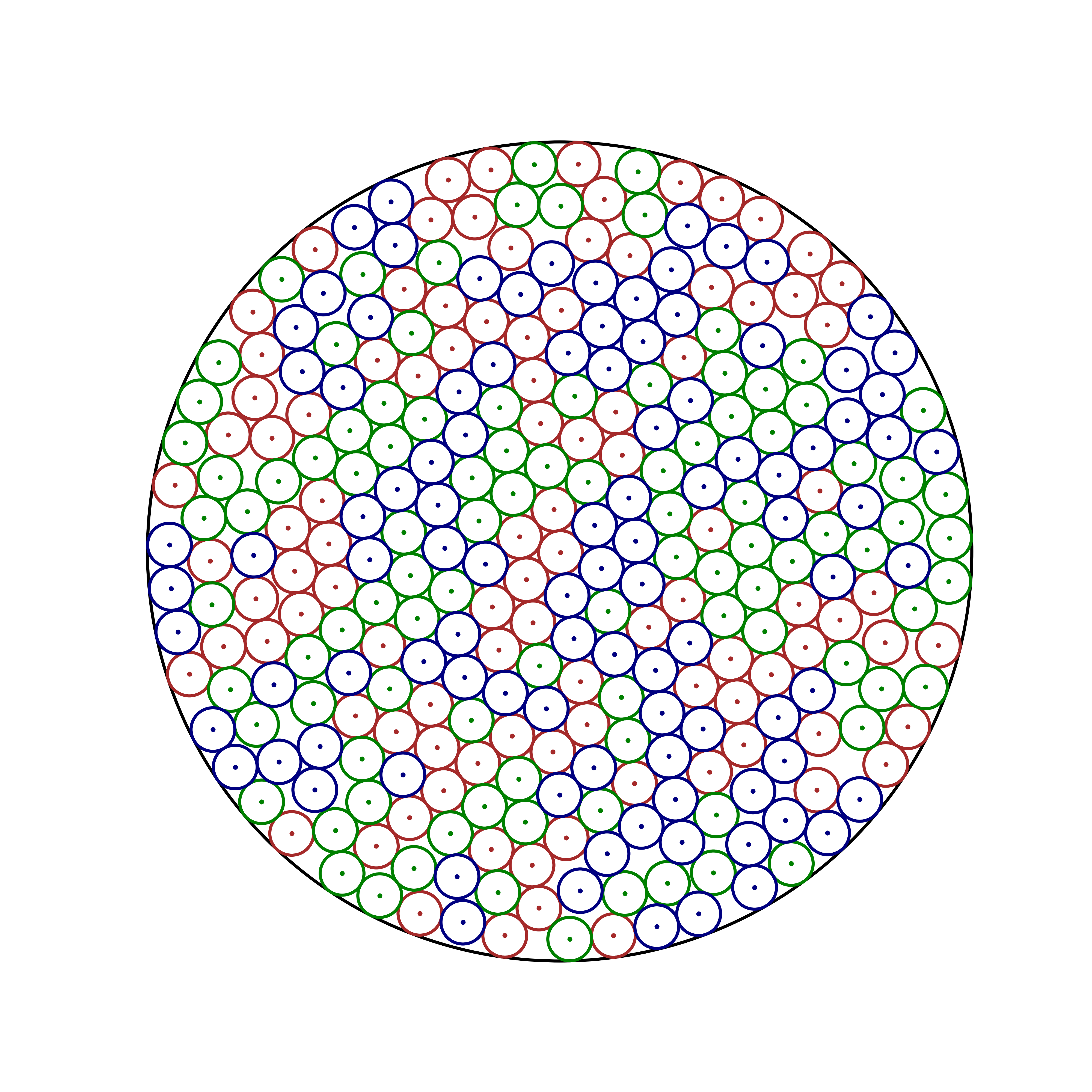
(d)

Figure 2: Illustration of the four partitions of the GBO method. The illustrative example has 300 circles ($n=300$), which is evenly partitioned into three batches ($k=3$) colored by three different colors where each batch having 100 circles.

In this way, the PECC problem is converted to an unconstrained non-convex continuous optimization problem with a fixed container radius. The pseudocode of our proposed GBO algorithm is presented in Algorithm 1. Given a candidate solution $\boldsymbol{x}$, a fixed container radius $R$, algorithm ${\rm GBO}(\boldsymbol{x},R)$ returns a solution $\boldsymbol{x}^{*}$ such that energy $E(\boldsymbol{x}^{*})$ reaches a local minimum. For this purpose, GBO first partitions the $n$ unit circles into $k$ batches (line 1), then GBO applies the BFGS method to minimize the energy on each batch iteratively (lines 6-11), the iteration process terminates when the maximum iteration step is reached (line 5) or the sum of the $L_{2}$-norm of $k$-batch gradients is tiny enough (lines 13-15). Finally, GBO returns a local minimum solution $\boldsymbol{x}^{*}$ obtained by merging the $k$-batch circles (line 17). Though it is hard to provide a mathematical analysis on the convergence of the proposed GBO algorithm, we observe that it always meets the convergence condition (line 13) when the maximum iteration step is set large enough.

To minimize the total computational complexity of the GBO method, each batch groups nearly the same number of circles. Concretely, the size of each batch is either $\lfloor\frac{n}{k}\rfloor$ or $\lceil\frac{n}{k}\rceil$. We provide several geometric $k$-batch partition strategies for solving the PECC problem, described as follows:

• 1) Sector (default): Sort all circles in the container in ascending order of the angle ${\theta}_{i}=\arctan{\frac{y_{i}}{x_{i}}}$, then partition them into $k$ subsets successively.

• 2) Annulus: Sort all circles in ascending order of the distance ${dis}_{i}=\sqrt{{x_{i}}^{2}+{y_{i}}^{2}}$, then partition them into $k$ subsets successively.

• 3) Fence: Sort all circles in ascending order of the coordinate $x_{i}$ , then partition them into $k$ subsets successively.

• 4) Random: Partition all circles into $k$ sets randomly.

Our experiments show that the sector partition outperforms other partitions, so the default partition is set as sector in this work. Figure 2 illustrates the above four partitions of the GBO method.

4.2 Optimization Method for Adjusting the Container

Starting from a random layout (all the circles are randomly placed in the container and overlapping is allowed), a local minimum solution is obtained by applying the GBO method, possibly containing overlaps and thus being infeasible. One strategy for obtaining a feasible solution is to expand the container radius and adjust the layout until the overlaps are eliminated. The most intuitive and common way to achieve this goal is to adopt the binary search (Huang and Ye, 2011; He et al., 2018). Recently, a smart and significantly faster method is proposed in (Lai et al., 2022) to find a feasible solution with a local minimum container radius $R$, which we present as follows.

Let vector $\boldsymbol{z}=[x_{1},y_{1},x_{2},y_{2},...,x_{n},y_{n},R]^{\mathrm{T}}$, $\boldsymbol{z}\in\mathbb{R}^{2n+1}$, be a candidate solution with the container radius $R$ as a variable. A new elastic energy $U$ can be reformulated as follows:

$$U(\boldsymbol{z},\lambda)=\sum_{i=1}^{n}\sum_{j=i+1}^{n}d_{ij}^{2}+\sum_{i=1}^{n}d_{i0}^{2}+\lambda R^{2},$$ (10)

where $\lambda R^{2}$ is a penalty term, and $\lambda$ is a penalty coefficient. By employing the optimization method to minimize the energy $U$, the container radius prefers to shrink when $\lambda$ increases, and it prefers to expand when $\lambda$ is decreasing. Therefore, the model converts the current goal to an unconstrained continuous optimization problem. By adjusting $\lambda$, it could allow to obtain a feasible solution when minimizing the energy $U$ with a local minimum container radius.

We adopt the main idea of adjusting container radius of (Lai et al., 2022) and control $\lambda R^{2}$ to minimize the container size. The pseudocode of our container radius adjusting method is depicted in Algorithm 2. Given a candidate solution $(\boldsymbol{x},R)$, Algorithm 2 initializes the coefficient $\lambda$ to an empirically fixed value $10^{-4}$ and combines $(\boldsymbol{x},R)$ to obtain a new candidate solution $\boldsymbol{z}$; then the algorithm performs several iterations to obtain a feasible solution. At each iteration, the algorithm employs the BFGS method to minimize the energy $U(\boldsymbol{z},\lambda)$ and updates the candidate solution $\boldsymbol{z}$. Then, the algorithm halves $\lambda$ and continually adjusts the candidate solution $\boldsymbol{z}$ at the next iteration. After several iterations, the energy $U(\boldsymbol{z},\lambda)$ converges to $0$, so that the overlaps are tiny enough and the candidate solution $\boldsymbol{z}$ can be regarded as a feasible solution with a local minimum container radius. Finally, the method returns the solution $(\boldsymbol{x}^{*},R^{*})$ as the result.

1 Input: A candidate solution $\boldsymbol{x}$ and the container radius $R$

Output: A feasible solution with local minimum container radius $(\boldsymbol{x}^{*},R^{*})$

1:  $\boldsymbol{z}^{*}\leftarrow\mathrm{combine}(\boldsymbol{x},R),\ \lambda\leftarrow 10^{-4}$

2:  for $t$ from $1$ to $35$ do

3:     employ BFGS to minimize the energy $U(\boldsymbol{z}^{*},\lambda)$

4:     $\lambda\leftarrow 0.5\times\lambda$

5:  end for

6:  $(\boldsymbol{x}^{*},R^{*})$ $\leftarrow$ $\mathrm{divide}(\boldsymbol{z}^{*})$

7:  return $(\boldsymbol{x}^{*},R^{*})$

Algorithm 2 adjust_container($\boldsymbol{x},R$)

Note that the term $\lambda R^{2}$ is tiny enough with sufficient iteration steps. The algorithm forces to converge the energy $E(\boldsymbol{x})=0$ ($U$ degenerates to $E$ without penalty term $\lambda R^{2}$) with non-fixed container radius.

4.3 The Neighbor Structure of Circles for Optimization

He et al. (2018) first propose an efficient neighbor structure, which can efficiently calculate the energies $E$ and $U$ and its gradient functions of a candidate solution, and the state-of-the-art algorithm IDTS (Lai et al., 2022) also adopts this method. In this subsection, we first introduce the neighbor structure. Then, we present our proposed ANM method and discuss the advantage of our method over the existing methods.

Let $l_{ij}$ denote the distance between the centers of two unit circles $c_{i}$ and $c_{j}$:

$$l_{ij}=\sqrt{(x_{i}-x_{j})^{2}+(y_{i}-y_{j})^{2}},$$

Recall that $d_{ij}$ denotes the energy between two unit circles $c_{i}$ and $c_{j}$ and is defined by Eq. (3). It is clear that $d_{ij}>0$ when $l_{ij}<2$, and $d_{ij}=0$ otherwise. We define the neighbor $\Gamma(i)$ of circle $c_{i}$ to be a subset of $n$ unit circles as follows, using a distance controlling hyperparameter $l_{cut}$:

$$\Gamma(i)=\left\{c_{j}\mid\forall j:1\leq j\leq n,\ i\neq j,\ l_{ij}<l_{cut}\right\},$$

When $l_{cut}=2$, all the circles $\{c_{j}\}$ overlapping with circle $c_{i}$ are contained in $\Gamma(i)$. Therefore the energies concerning circle $c_{i}$ can be calculated by enumerating the circles $c_{j}$ in $\Gamma(i)$ instead of enumerating all the packing circles. So, the batch energy $E$ (Eq. (5)) and the energy $U$ (Eq. (10)) can be reformulated as follows:

$$E(\boldsymbol{x}_{p})=\sum_{i\in B_{p}}\sum_{j\in\Gamma(i)}d_{ij}^{2}[j\notin B_{p}\vee j<i]+\sum_{i=1}d_{i0}^{2},$$

$$U(\boldsymbol{z},\lambda)=\sum_{i=1}^{n}\sum_{j\in\Gamma(i)}d_{ij}^{2}[j<i]+\sum_{i=1}^{n}d_{i0}^{2}+\lambda R^{2},$$

Note that the statements “$j\notin B_{p}\vee j<i$” and “$j<i$” guarantee the circle-circle overlaps be calculated only once.

However, when $l_{cut}=2$, the neighbor structure needs to be maintained even if the circles have minor shifts in the layout, otherwise, the correctness of the energy and gradient computation can not be guaranteed. Therefore, if we properly increase the value of $l_{cut}$, more adjacent circles are contained in the neighbor, so that the correctness is guaranteed without maintaining the neighbor structure when the circles have minor shifts in the layout. But if $l_{cut}$ is set too large, the neighbor contains many unnecessary circles, increasing the time cost of the energy and gradient computation. Therefore, we empirically set $l_{cut}=4$ as a trade-off setting. Figure 3 gives an example to show the neighbors of a circle and the different settings of $l_{cut}$. Note that calculating the energies $E$ and $U$ and their gradients by enumerating the pairwise circles is of $O(n^{2})$ complexity. By adopting the neighbor structure, the complexity can be reduced to $O(n)$ (He et al., 2018).

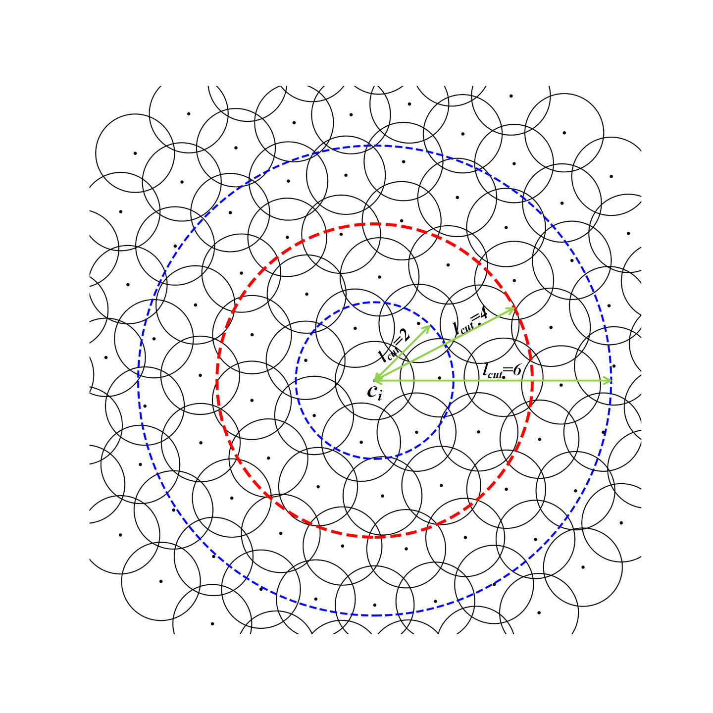
Figure 3: Illustration of the neighbors of a circle with different $l_{cut}$ settings. This illustrative example gives three settings for $l_{cut}=$ 2, 4 or 6 on a conflicting layout. We empirically set $l_{cut}=4$ as a trade-off setting in this work.

1 Input: A deferring counter $cnt$; A deferring length $len$; A neighbor $\Gamma$

Output: An updated counter $cnt$; A updated length $len$; A updated neighbor $\Gamma$

1:  $cnt\leftarrow cnt+1$

2:  if $cnt\geq len$ then

3:     construct the current neighbor $\Gamma^{\prime}$

4:     if $\Gamma\neq\Gamma^{\prime}$ then

5:        $cnt\leftarrow 0,\ len\leftarrow 1,\ \Gamma\leftarrow\Gamma^{\prime}$

6:     else

7:        $cnt\leftarrow 0,\ len\leftarrow 2\times len$

8:     end if

9:  end if

10:  return $(cnt,len,\Gamma)$

Algorithm 3 ANM ($cnt,len,\Gamma$)

Our proposed ANM method is depicted in Algorithm 3. ANM maintains three parameters, i.e., the counter $cnt$, deferring length $len$, and historical neighbor $\Gamma$. Initially, the counter is set to $0$, the length is set to $1$, and the algorithm calculates an initial neighbor $\Gamma$ (refer to Algorithm 1 lines 3-4). In the continuous optimization process, the ANM is called after each iteration (see in Algorithm 1 line 12), and the counter will increase by $1$ when ANM is called. If the counter $cnt$ equals the deferring length $len$, ANM reconstructs a new neighbor $\Gamma^{\prime}$ and compares it with the historical neighbor $\Gamma$. If two neighbors $\Gamma^{\prime}$ and $\Gamma$ are the same, the counter is set to $0$ and the deferring length $len$ is multiplied by $2$, otherwise, the counter is set to $0$, the deferring length is set to $1$ and the neighbor $\Gamma$ is updated by $\Gamma^{\prime}$.

The basic idea of ANM to defer maintaining the neighbor structure is based on the operation of the counter $cnt$ and the deferring length $len$. If the layout is unstable and the neighbor is changed, ANM reconstructs the neighbor in every iteration. If the layout is stable, the deferring length $len$ grows exponentially, which makes ANM defers maintaining the neighbor. It is worth noting that the Voronoi diagram approach can also be used to construct the neighbor, which can gain an excellent time complexity $O(n\log n)$. In this work, we adopt the scan line approach ($O(n\sqrt{n})$) to construct the neighbor, which is efficient enough and easy to implement.

He et al. (2018) use a simple strategy to maintain the neighbor, consisting in reconstructing the neighbor every 10 iterations. However, reconstructing the neighbor is unnecessary when the layout is stable, and it will waste computational resources in this case. Lai et al. (2022) propose a two-phase strategy. In the first phase, they calculate the energy and gradient by enumerating all the pairwise circles without using the neighbor structure. When the condition $\|g(\boldsymbol{x})\|_{\infty}<10^{-2}$ is met, they change to the second phase. In the second phase, they construct the neighbor structure only at the beginning of the phase; then they use the neighbor structure to obtain the energy and gradient until the algorithm finds a local minimum solution. This two-phase strategy has three disadvantages: 1) The enumeration method in the first phase is computationally expensive, especially on large scale instances. 2) The threshold of the condition needs to be fine-tuned on the different scales of instances. 3) The neighbor structure is not updated in the second phase, so that if the solution falls into a saddle point, the correctness of this strategy can not be guaranteed. Our ANM method can well handle these issues.

It is worth mentioning that our ANM is an adaptive method, ANM can handle dynamic problems where the number and the radius of the packing items can be changed, such as the online packing problems (Hokama et al., 2016; Fekete and Hoffmann, 2017; Fekete et al., 2019; Lintzmayer et al., 2019).

4.4 The Complexity Analysis of GBO

We now provide the time and space complexity analysis of our GBO based on the BFGS optimization method.

Time complexity. We analyze the time complexity of each iteration. From Algorithm 1 lines 6 to 15, it is obvious that each iteration has 6 components, including the batch gradient $g(\boldsymbol{x}_{p})$ calculation, the batch step length $\alpha_{p}$ calculation, the batch vector $\boldsymbol{x}_{p}$ update, the batch Hessian matrix $\boldsymbol{H}_{p}$ update, the maintenance module ANM, and the sum of the $k$-batch gradient norm. Since we adopt the efficient neighbor structure (He et al., 2018) (discussed in Section 4.3), the energy and gradient functions can be executed in time complexity $O(n)$. So, the time complexity of the batch gradient calculation, the step length calculation and the sum of $k$-batch gradient norm is $O(\frac{n}{k})$, $O(\beta\frac{n}{k})$ and $O(n)$, respectively, where the constant $\beta$ approximates the recursion depth of line search approach. Each batch has $\frac{n}{k}$ packing items, so the size of the batch Hessian matrix is $O((\frac{n}{k})^{2})$. The batch vector update (Eq. (6)) and the batch Hessian matrix update (Eqs. (8) and (9)) involve matrix and vector multiplication, so both of their time complexity are $O((\frac{n}{k})^{2})$. We employ the scan line approach to construct the neighbor structure in the ANM module (discussed in Section 4.3), its time complexity is $O(n\sqrt{n})$ (using Voronoi diagram approach can gain a better time complexity of $O(n\log{n})$). Finally, the time complexity of each iteration is $O(k(\frac{n}{k}+\beta\frac{n}{k}+(\frac{n}{k})^{2})+n+n\sqrt{n})$, which can be simplified as $O(\beta{n}+n\sqrt{n}+\frac{n^{2}}{k})$, and it becomes $O(\beta{n}+\frac{n^{2}}{k})$ if the ANM module defers the maintaining process.

Space complexity. The memory requirement of the GBO method is mainly used to store the $k$ batch Hessian matrices. Therefore, the space complexity of the GBO method is $O(k(\frac{n}{k})^{2})$, which can be simplified as $O(\frac{n^{2}}{k})$.

As discussed above, our GBO method has lower time and space complexity ($O(\beta{n}+\frac{n^{2}}{k})$ and $O(\frac{n^{2}}{k})$) than the classic BFGS method ($O(n^{2})$ and $O(n^{2})$). It degenerates to the BFGS method when $k=1$.

5 Search Heuristic

1 Input: A number of unit circles $n$; A best-known container radius $R_{b}$; The cut-off time $T_{cut}$

Output: A feasible solution with the minimal container radius $(\boldsymbol{x}^{*},R^{*})$

1:  $\boldsymbol{x}^{*}\leftarrow\mathrm{random\_solution}(n,R_{b})$

2:  $\boldsymbol{x}^{*}\leftarrow\mathrm{GBO}(\boldsymbol{x}^{*},R_{b})$

3:  $(\boldsymbol{x}^{*},R^{*})\leftarrow\mathrm{adjust\_container}(\boldsymbol{x}^{*},R_{b})$

4:  while $\mathrm{time}()\leq T_{cut}$ do

5:     $R\leftarrow\min(R_{b},R^{*})$

6:     $\boldsymbol{x}\leftarrow\mathrm{SED}(n,R)$

7:     $(\boldsymbol{x},R)\leftarrow\mathrm{adjust\_container}(\boldsymbol{x},R)$

8:     if $R<R^{*}$ then

9:        $\boldsymbol{x}^{*}\leftarrow\boldsymbol{x},\ R^{*}\leftarrow R$

10:     end if

11:  end while

12:  return $(\boldsymbol{x}^{*},R^{*})$

Algorithm 4 The framework for solving PECC

The algorithms for solving the PECC problem based on the elastic model can be divided into two phases. In the first phase, the container radius is fixed, and the goal is to find a feasible solution or an infeasible solution with as few overlaps as possible (i.e., the energy $E$ being as minimal as possible). In the second phase, the algorithms expand or shrink the container radius to obtain a feasible solution with the container radius being as minimum as possible. Starting from a random candidate solution, although we can obtain a feasible solution by employing the GBO method (Section 4.1) to accomplish the first phase and employing the container adjustment method (Section 4.2) to accomplish the second phase. However, the quality of the solution obtained in this way is still unsatisfactory.

Through sufficient experiments, we observe that the quality of the final solution is directly impacted by the solution obtained in the first phase. If the energy $E(\boldsymbol{x})$, corresponding to the overlapping area, of the obtained solution in the first phase is large, the expanded difference of the radius adjustment in the second phase is also large. On the other hand, if a feasible solution is found in the first phase, the radius can be shrunk in the second phase. Therefore, a minimum energy solution discovered in the first phase is important to obtain a final high-quality feasible solution. However, the elastic model converts the PECC problem to a non-convex optimization problem as discussed in Section 3.2, and it is extremely difficult to find a global minimum solution. Therefore, we propose an efficient Solution-space Exploring and Descent (SED) heuristic for the first phase to discover a solution with as minimum energy as possible.

5.1 The Framework for Solving PECC

We first introduce our algorithm framework, of which the pseudocode is depicted in Algorithm 4.

Initially, the algorithm adopts the best-known radius (Specht, 2022) $R_{b}$ as the initial fixed container radius and generates a random layout as the initial solution (line 1). The center $(x_{i},y_{i})$ of each circle satisfies $x_{i},y_{i}\in\mathcal{U}(-R_{b},R_{b})$ ($\mathcal{U}$ is denoted as the continuous uniform distribution). Then, the algorithm employs our GBO method (Section 4.1) to minimize the energy $E(\boldsymbol{x}^{*})$ (line 2) to obtain an initial feasible solution $\boldsymbol{x}^{*}$ (line 3) by employing the container adjusting method (Section 4.2). Next, the algorithm performs an iterative process to improve the best recorded solution until the cutoff time $T_{cut}$ is reached (lines 4-11).

At each iteration, the algorithm sets the target radius $R$ as min($R_{b}$, $R^{*}$) (line 5), where $R_{b}$ is the best-known radius $R_{b}$ and $R^{*}$ is the best feasible radius $R^{*}$ found so far. Then, it adopts our proposed SED heuristic (Section 5.2) to discover a candidate solution $\boldsymbol{x}$ with as low energy as possible (line 6). Subsequently, the algorithm computes a new feasible solution by applying the container radius adjusting method to the candidate solution (line 7). If the new feasible radius is smaller than the best recorded radius, indicating a better feasible solution is found, then the best record solution is updated (lines 8-10). Finally, the algorithm returns the best recorded solution as the result.

Note that our goal is to solve large scale instances, which is an incredibly big computational challenge. Using the best-known radius instead of an approximate radius or a radius obtained by an initial method as the baseline can reduce the computational difficulty, quickly discover a high-quality solution and improve the algorithm performance. Therefore, it is an efficient quick-start method.

5.2 The Solution-Space Exploring and Descent Heuristic

Our proposed SED heuristic aims to solve a problem described as follows. Given a fixed container radius, the problem determines whether there is a feasible solution, and it is essentially a decision PECC problem. If SED discovers a feasible solution, it returns the solution immediately; otherwise, it returns an infeasible solution with the smallest energy during the search process. First, we define a new metric function $J$, formulated as follows:

$$J(\boldsymbol{x})=\lceil-\log_{10}E(\boldsymbol{x})\rceil,$$

where function $J$ is the ceiling of the negative logarithm of the function $E$. It maps the energy $E$ to an integer. And the value of function $J$ is applied to control the exploring number in the heuristic process.

1 Input: A number of unit circles $n$; A container radius $R$

Output: A smallest energy solution found so far $\boldsymbol{x}^{*}$

1:  $\boldsymbol{x}\leftarrow\mathrm{random\_solution}(n,R)$

2:  $\boldsymbol{x}\leftarrow\mathrm{GBO}(\boldsymbol{x},R)$

3:  $\boldsymbol{x}^{*}\leftarrow\boldsymbol{x}$

4:  for $i$ from $1$ to $S_{iter}$ do

5:     if $E(\boldsymbol{x}^{*})\leq 10^{-25}$ then

6:        break

7:     end if

8:     $m\leftarrow\max(1,J(\boldsymbol{x})),\ U\leftarrow\emptyset$

9:     for $j$ from $1$ to $m$ do

10:        $\boldsymbol{x}^{\prime}\leftarrow\mathrm{perturbing}(\boldsymbol{x})$

11:        $\boldsymbol{x}^{\prime}\leftarrow\mathrm{GBO}(\boldsymbol{x}^{\prime})$

12:        $U\leftarrow U\cup\{\boldsymbol{x}^{\prime}\}$

13:     end for

14:     $\boldsymbol{x}\leftarrow\mathrm{select}(U)$

15:     if $E(\boldsymbol{x})<E(\boldsymbol{x}^{*})$ then

16:        $\boldsymbol{x}^{*}\leftarrow\boldsymbol{x}$

17:     end if

18:  end for

19:  return $\boldsymbol{x}^{*}$

Algorithm 5 SED($n$, $R$)

Now, we introduce our proposed SED heuristic depicted in Algorithm 5. Starting from a fixed container radius $R$, SED first generates a random configuration as the initial solution and minimizes the energy of the initial solution $\boldsymbol{x}$ by adopting our GBO method (lines 1-2). Then, SED performs an iterative process to discover a feasible solution (lines 4-18). At each iteration, SED obtains a value $m$ by function $J$ as the perturbing number (line 8), a candidate solution set $U$, $|U|=m$, is created where the candidate solution $\boldsymbol{x}^{\prime}$ in $U$ is obtained by perturbing the current operated solution $\boldsymbol{x}$ and minimizing energy $E(\boldsymbol{x}^{\prime})$ by adopting GBO (lines 9-13). Then SED adopts a $select$ operator to choose a candidate solution from set $U$ to replace the solution $\boldsymbol{x}$. If the energy of new solution $\boldsymbol{x}$ is smaller than the energy of the best record solution $\boldsymbol{x}^{*}$, then $\boldsymbol{x}^{*}$ is updated (lines 15-17). If the energy of $\boldsymbol{x}^{*}$ is tiny enough, indicating a feasible solution is discovered, SED returns the feasible solution $\boldsymbol{x}^{*}$ immediately (lines 5-7), otherwise, SED returns an infeasible solution with the smallest energy during the iteration process when reaching the maximum number of iteration steps $S_{iter}$.

To obtain a perturbed solution $\boldsymbol{x}^{\prime}$, we randomly shift the coordinate of the circles in the operated solution $\boldsymbol{x}$ which can be described as follows, $x^{\prime}_{i}\leftarrow x_{i}+r$ and $y^{\prime}_{i}\leftarrow y_{i}+r\ \ (1\leq i\leq n)$, where $r$ is a random number, $r\in\mathcal{U}(-0.8,0.8)$.

The strategy of the $select$ operator is described as follows:

$$\mathrm{select}(U)=\begin{cases}\underset{\boldsymbol{y}\in U}{\arg\min}\ E(\boldsymbol{y}),&\mathrm{if}\ \ \underset{\boldsymbol{y}\in U}{\min}\ E(\boldsymbol{y})<E(\boldsymbol{x})\\ P\left(X=\boldsymbol{y}\mid p_{\boldsymbol{y}}=softmax(J(\boldsymbol{y}))\right),&\mathrm{otherwise}\end{cases}$$

$$softmax(J(\boldsymbol{y}))=\frac{\exp(J(\boldsymbol{y}))}{\sum_{\boldsymbol{y}^{\prime}\in U}\exp(J(\boldsymbol{y}^{\prime}))}.$$

This operator first compares the candidate solution with the smallest energy in set $U$ to the current operated solution $\boldsymbol{x}$. If the energy of the candidate solution is smaller than the operated solution, the operator replaces the operated solution as the candidate solution; otherwise, the operator selects a candidate solution from set $U$ according to the probability of the softmax function.

6 Experiments

For experiments, we first evaluate the performance of our proposed GBO method on the different number of batches and different geometric partition methods, then we present the comparisons between the results and also give the parameter studies.

6.1 Experimental Setup

Our algorithm was implemented in C++ and compiled using g++ 5.4.0. Experiments were performed on a server with Intel® Xeon® E5-2650 v3 CPU and 256 GBytes RAM, running the Linux OS. Due to the randomness, we run our algorithm multiple times independently with different random seeds (CPU timestamps). To evaluate the performance of our algorithm thoroughly, we select three instance scales as our benchmarks, described as follows:

• Moderate scale: $300\leq n\leq 320$, for comparing with the state-of-the-art algorithm IDTS (Lai et al., 2022). We set $k=3$ for the batch number of GBO, 12 hours for cut-off time $T_{cut}$ of our overall search. The algorithm performs 20 times independently, where the settings of cut-off time and performing time are the same as in the IDTS work.

• Large scale I: $500\leq n<800$, for comparing with the best-known results (Specht, 2022). We set $k=5$ for the batch number, 24 hours for cut-off time $T_{cut}$. The algorithm performs 10 times independently.

• Large scale II: $800\leq n\leq 1000$, for comparing with the best-known results (Specht, 2022). We set $k=5$ for the batch number, 48 hours for cut-off time $T_{cut}$. The algorithm performs 10 times independently.

The rest of the parameters are consistently set as follows. The geometrical partition method is sector (Section 4.1), the maximum iteration steps of GBO $MaxIter=5000$ (Section 4.1), and the maximum iteration steps of SED $S_{iter}=500$ (Section 5.2). The parameters tuning and analysis are presented in Section 6.5.

6.2 Comparison on the Well-Studied Moderate Scale Instances

Table 1: Comparison between the best-known results, IDTS and our proposed algorithms SED (1-batch GBO) and (5-batch GBO) on the 21 well-studied moderate scale instances. The improved best results $R_{best}$ found by our proposed algorithms appear in bold.

$n$	$R^{*}$		IDST		SED (1-batch GBO)												SED (3-batch GBO)
					$R_{best}$		$R_{avg}$		$R_{best}-R^{*}$		$RR$		$HR$		$time\leavevmode\nobreak\ (s)$		$R_{best}$		$R_{avg}$		$R_{best}-R^{*}$		$RR$		$HR$		$time\leavevmode\nobreak\ (s)$
300	18.813153706		18.813153706		18.813157576		18.813191071		3.87E-06		0/20		1/20		26216		18.813189941		18.813198345		3.62E-05		0/20		12/20		33237
301	18.843463507		18.843463507		18.843463507		18.844498079		0.00E+00		2/20		2/20		26222		18.843463507		18.843551084		0.00E+00		1/20		1/20		38618
302	18.891782255		18.891782255		18.891781604		18.892064228		-6.51E-07		2/20		1/20		20792		18.891782255		18.892033313		0.00E+00		2/20		2/20		23987
303	18.929749153		18.929749153		18.929749153		18.930326363		0.00E+00		1/20		1/20		23549		18.929750618		18.930328723		1.47E-06		0/20		1/20		23652
304	18.964441751		18.964441751		18.964297557		18.964819754		-1.44E-04		3/20		1/20		24562		18.963620323		18.964664008		-8.21E-04		5/20		1/20		18852
305	19.001754565		19.001754565		19.001744832		19.002856526		-9.73E-06		1/20		1/20		24542		19.001726813		19.002734687		-2.78E-05		2/20		1/20		21922
306	19.030389407		19.030389407		19.031079983		19.031763629		6.91E-04		0/20		1/20		21131		19.030651242		19.031391719		2.62E-04		0/20		2/20		25226
307	19.060160922		19.060160922		19.061100857		19.062150163		9.40E-04		0/20		1/20		23579		19.060841920		19.061955433		6.81E-04		0/20		1/20		26981
308	19.104991437		19.104991437		19.109083748		19.110722905		4.09E-03		0/20		1/20		26804		19.107239953		19.109820607		2.25E-03		0/20		1/20		23291
309	19.142573165		19.142573165		19.141335827		19.143371324		-1.24E-03		5/20		1/20		25662		19.142625039		19.143620434		5.19E-05		0/20		1/20		24278
310	19.178928265		19.178928265		19.178560517		19.179857308		-3.68E-04		2/20		1/20		18906		19.178419320		19.179442843		-5.09E-04		6/20		1/20		24718
311	19.212365036		19.212365036		19.210669807		19.213148503		-7.17E-04		5/20		1/20		22109		19.210564074		19.212561780		-8.22E-04		4/20		2/20		21153
312	19.233585653		19.233585653		19.233585653		19.234863780		0.00E+00		1/20		1/20		23934		19.233585653		19.234529499		0.00E+00		4/20		4/20		30386
313	19.257103014		19.257103014		19.256994660		19.258015876		-1.08E-04		1/20		1/20		21251		19.257103014		19.258284406		0.00E+00		1/20		1/20		25457
314	19.286195141		19.286195141		19.286190236		19.286514591		-4.91E-06		4/20		4/20		25125		19.286190236		19.286476954		-4.91E-06		1/20		1/20		26386
315	19.302288067		19.302288067		19.302273991		19.302586043		-1.41E-05		17/20		11/20		25517		19.302273991		19.302286175		-1.41E-05		18/20		3/20		24488
316	19.334041754		19.334041754		19.334041754		19.334805176		0.00E+00		9/20		9/20		25370		19.334041754		19.334584281		0.00E+00		7/20		7/20		22840
317	19.367595672		19.367595672		19.367595672		19.367930543		0.00E+00		10/20		10/20		23713		19.367595672		19.367871121		0.00E+00		9/20		9/20		23129
318	19.391566091		19.391566091		19.391566091		19.391909306		0.00E+00		15/20		15/20		22836		19.391566091		19.391631572		0.00E+00		17/20		17/20		27084
319	19.424277830		19.424277830		19.424277830		19.424920970		0.00E+00		15/20		15/20		18382		19.424277830		19.425310867		0.00E+00		12/20		12/20		24782
320	19.456230764		19.451649630		19.451583741		19.453206681		-4.65E-03		20/20		1/20		27713		19.451734176		19.454455527		-4.50E-03		19/20		3/20		30039
#Improve					10												6
#Equal					7												8
#Worse					4												7

We perform our proposed SED (3-batch GBO) algorithm and its variant SED (1-batch GBO) on the moderate scale instances ($300\leq n\leq 320$). The comparisonal results of two algorithms with best-known results (Specht, 2022) and IDTS (Lai et al., 2022) are shown in Table 1. Note that SED (1-batch GBO) only changes the number of batches from $k=3$ to $k=1$ for SED (3-batch GBO), and the 1-batch GBO degenerates to the classic BFGS method.

In Table 1, $n$ corresponds to the number of items in the instance, $R^{*}$ is for the best-known results from the Packomania website (Specht, 2022) (download data 2022/10/1), followed by the best results of IDTS (Lai et al., 2022). SED (1-batch GBO) and SED (3-batch GBO) correspond to the results of our methods: $R_{best}$ shows the best result of 20 independent runs, $R_{avg}$ shows the average result of 20 independent runs, $R_{best}-R^{*}$ is the difference between $R_{best}$ and $R^{*}$ (a negative value indicates an improved best result), $RR$ is the ratio of better than or equal to the best-known result $R^{*}$, $HR$ is the ratio of hitting the best value $R_{best}$, and $time\leavevmode\nobreak\ (s)$ shows the average time of obtaining a best solution in seconds. At the bottom of the table, “#Improve”, “#Equal” and “#Worse” indicates that for our two algorithms SED (1-batch GBO) and SED (3-batch GBO), the number of instances that our algorithm obtained better, equal, or worse result than the best of $R^{*}$ and IDTS.

From Table 1, we can draw several conclusions as follows:

• Our proposed heuristic SED with 1-batch GBO (i.e., classic BFGS) has 10 improved best results, 7 equal best results and 4 worse best results to IDTS on the 21 moderate scale instances. It demonstrates that SED outperforms IDTS. Note that the best-known results are same as IDTS, excluding $n=320$, and IDTS adopts L-BFGS as the optimization method, which is also a Quasi-Newton method.

• SED (3-batch GBO) has 6 improved best results, 8 equal best results and 7 worse best results on the 21 moderate scale instances. The results show that the 3-batch GBO does not outperform the 1-batch GBO (classic BFGS method). It implies the multi-batch GBO does not work well on moderate scale instances.

• From the ratio of hitting the best result $R_{best}$ ($HR$), there are few ratios of $HR$ high than 10/20, the most of the ratios of HR are equal to 1/20. From the IDTS work, we also observe that all the ratios of $HR$ in the IDTS work for $300\leq n\leq 320$ are less than 6/20, and there are 14 ratios of $HR$ equal to 1/20. These results demonstrate the moderate scale instances are well-studied and obtaining an improved best result is very difficult.

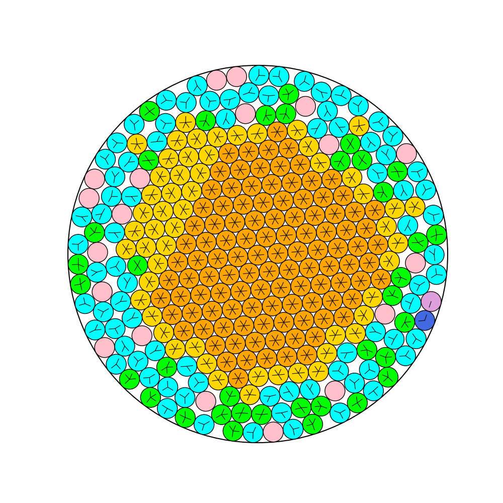
(a)

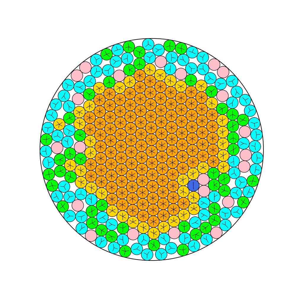
(b)

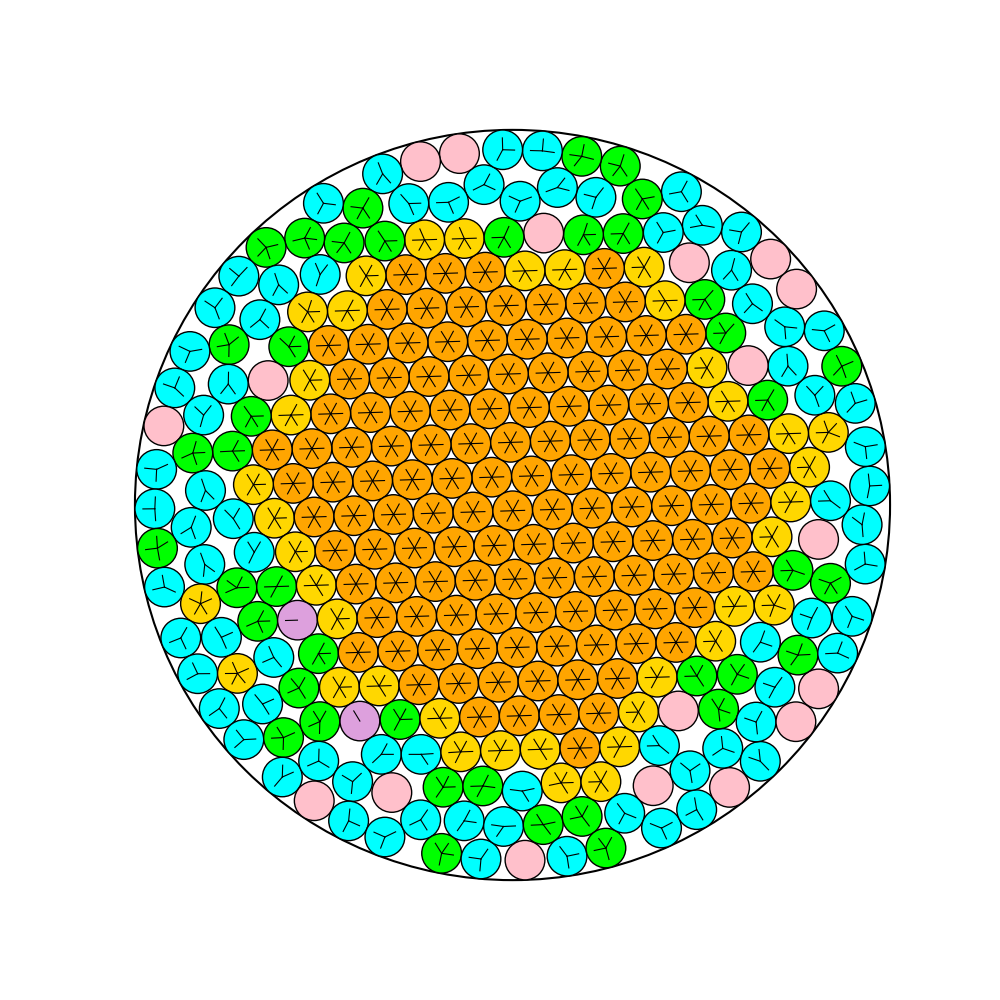
(c)

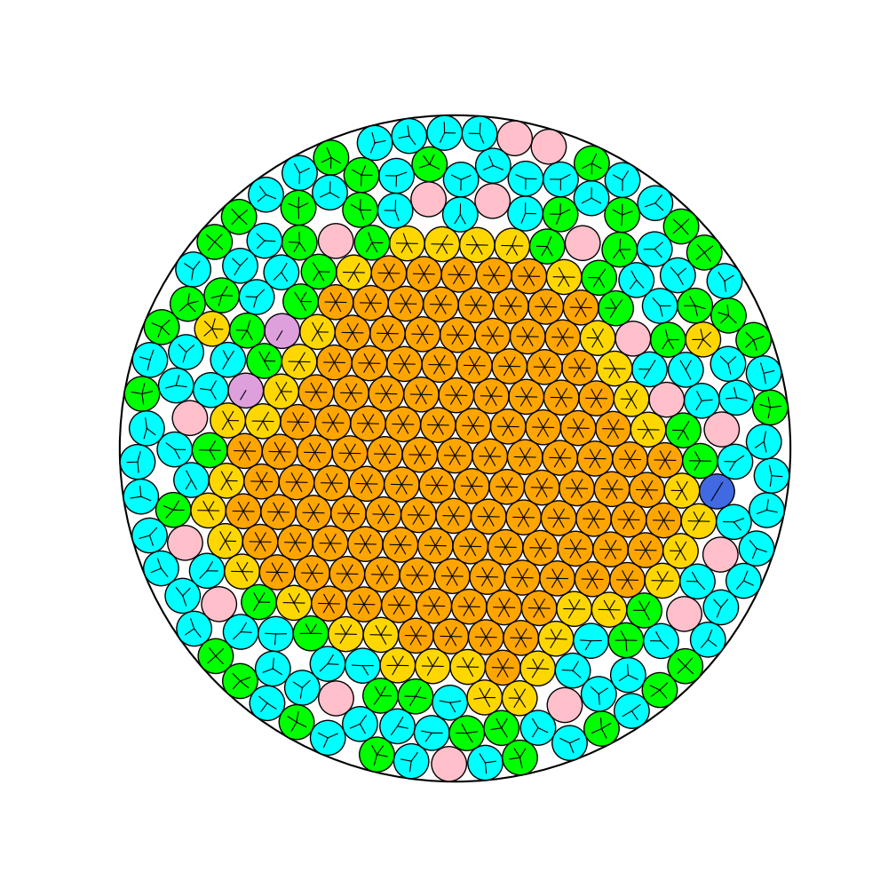
(d)

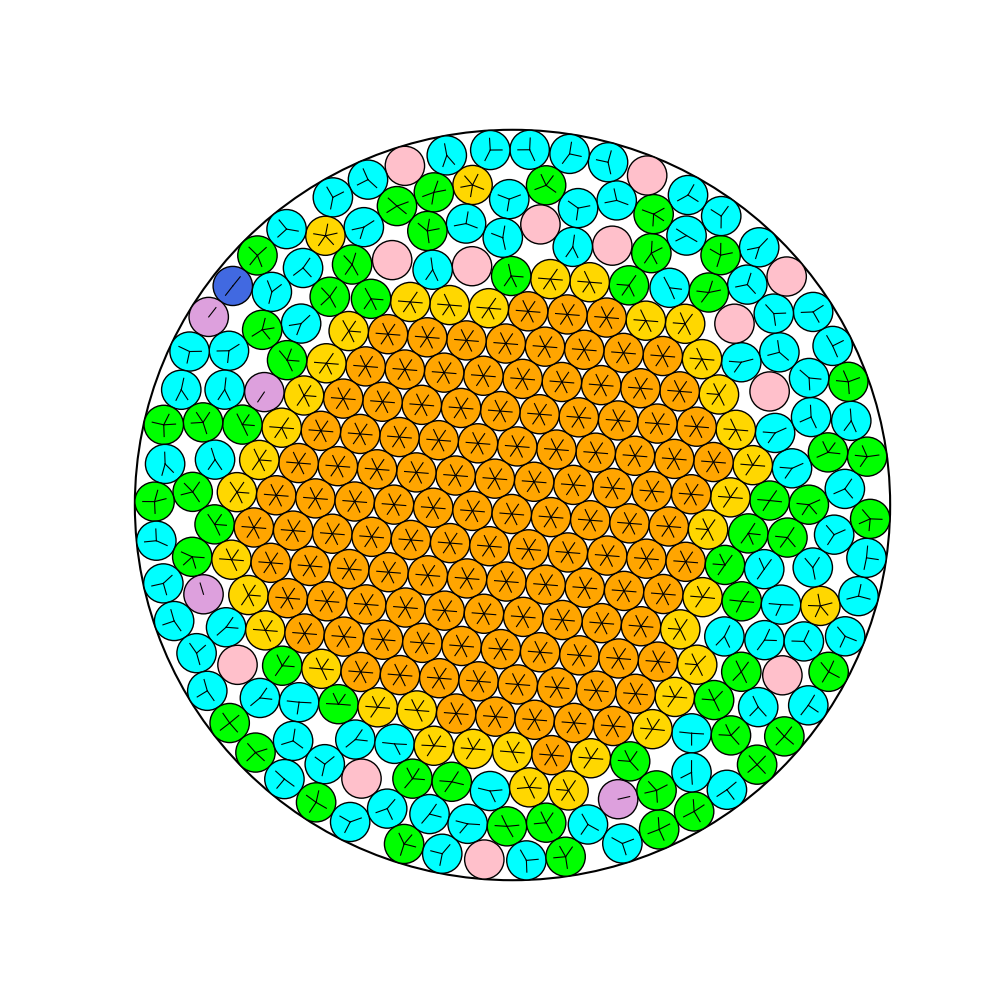
(e)

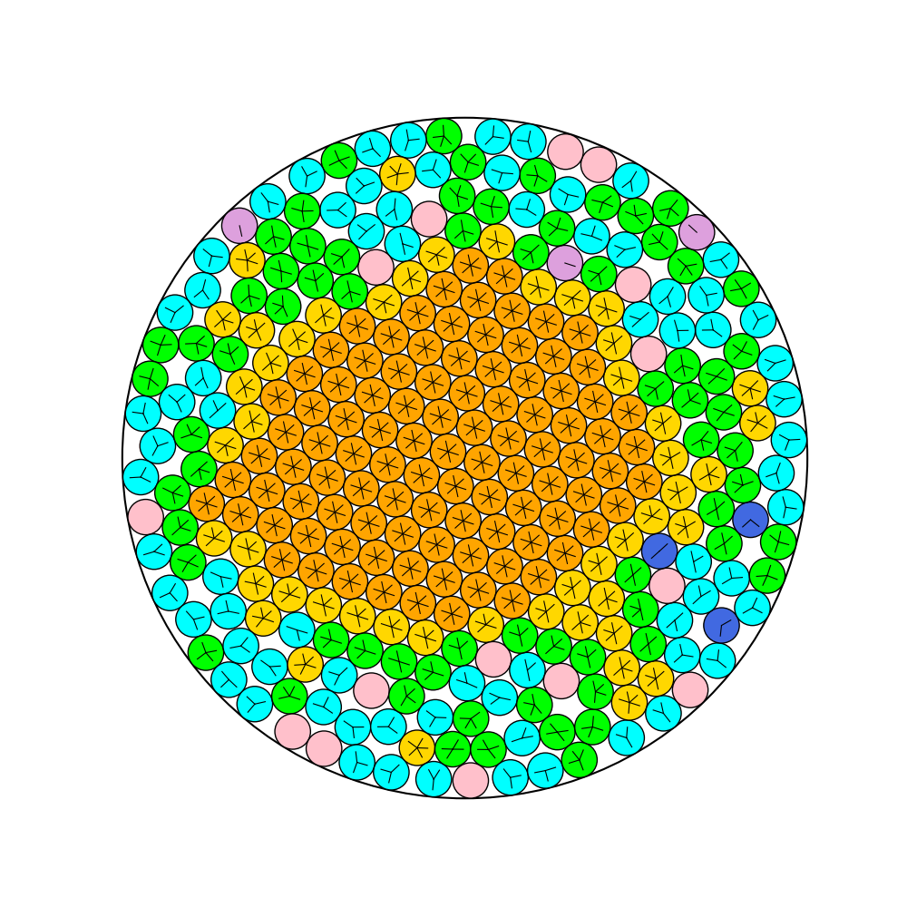
(f)

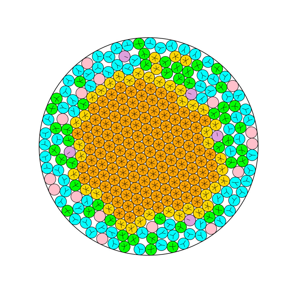
(g)

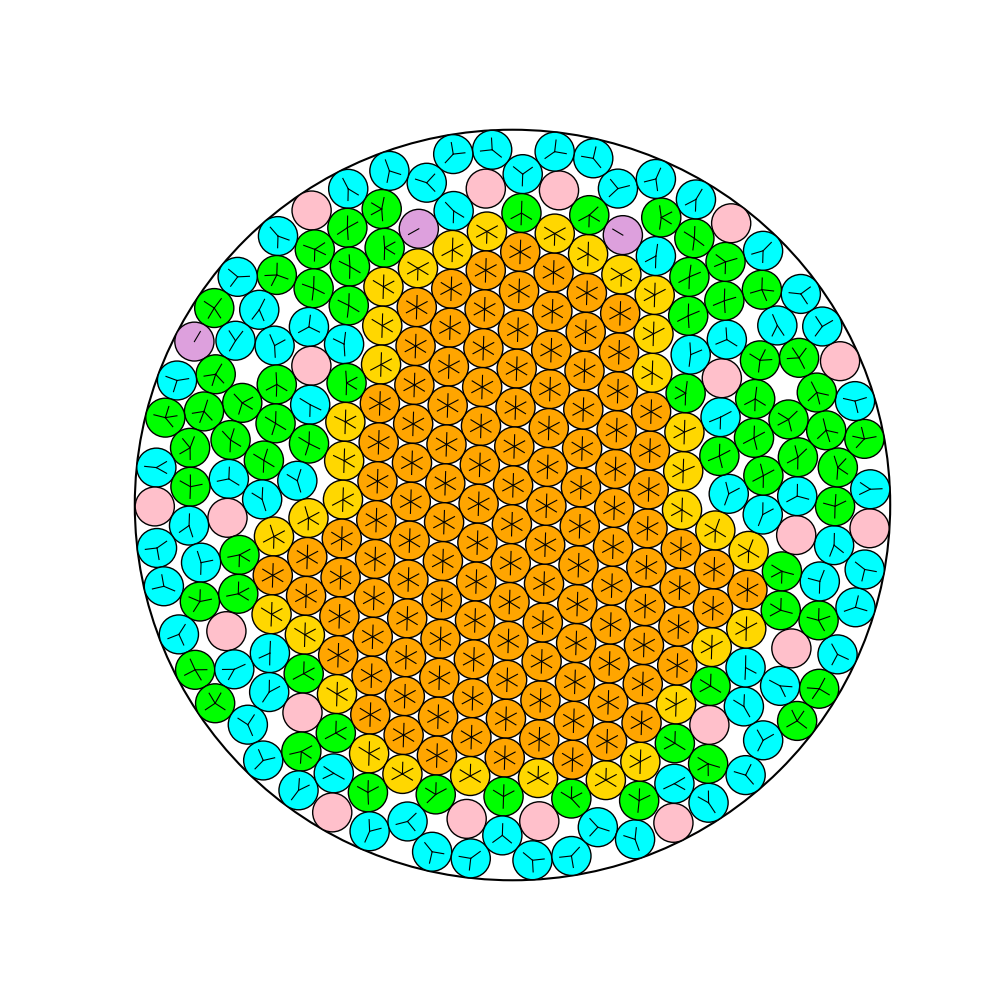
(h)

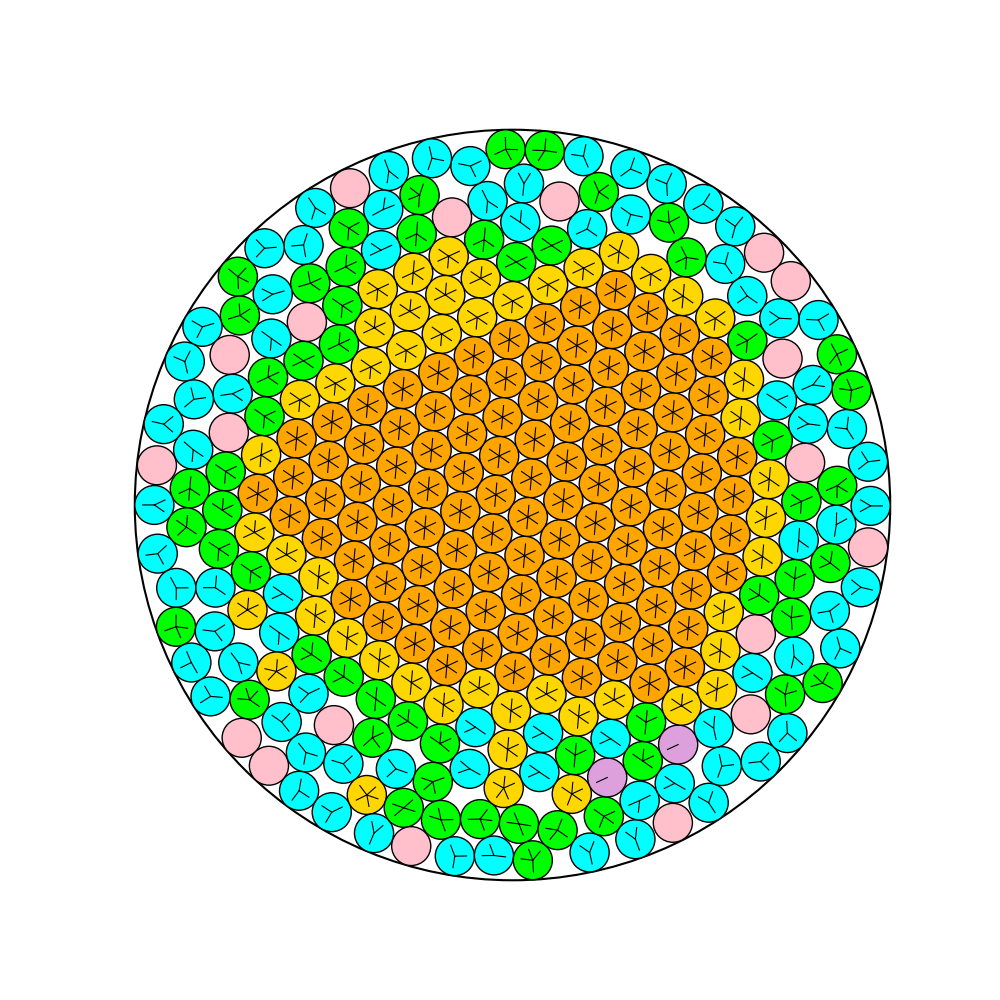
(i)

Figure 4: New improved solutions found by our proposed algorithm on the moderate scale instances $(300\leq n\leq 320)$. The circles are colored by various colors according to the number of contact circles, where two circles $c_{i}$ and $c_{j}$ are considered to contact each other if the distance $d(c_{i},c_{j})$ between two circle centers satisfies $d(c_{i},c_{j})\leq 2+10^{-10}$.

6.3 Comparison on Large Scale Instances

Table 2: Comparison between the best-known results and SED (5-batch GBO) on the 51 large scale instances of the regular number. The improved best results of $R_{best}$ and $R_{avg}$ appear in bold.

$n$	$R^{*}$		SED (5-batch GBO)														$n$	$R^{*}$		SED (5-batch GBO)
			$R_{best}$		$R_{avg}$		$R_{best}-R^{*}$		$RR$		$HR$		$time\leavevmode\nobreak\ (s)$							$R_{best}$		$R_{avg}$		$R_{best}-R^{*}$		$RR$		$HR$		$time\leavevmode\nobreak\ (s)$
500	24.1329376240		24.1312529426		24.1313788210		-1.68E-03		10/10		1/10		39561				800	30.4212133790		30.4198645288		30.4250741893		-1.35E-03		2/10		1/10		132389
510	24.4365629292		24.4210537570		24.4249135890		-1.55E-02		10/10		1/10		60259				810	30.6017659657		30.5956736421		30.6002028281		-6.09E-03		6/10		1/10		92738
520	24.6609522831		24.6258073657		24.6314124118		-3.51E-02		10/10		1/10		69426				820	30.7666908826		30.7489836784		30.7533477503		-1.77E-02		10/10		1/10		125921
530	24.8482376878		24.8455280225		24.8472603022		-2.71E-03		7/10		1/10		44648				830	30.9418117602		30.9297617239		30.9337956547		-1.21E-02		10/10		1/10		116582
540	25.0884399378		25.0855911217		25.0877127273		-2.85E-03		8/10		1/10		45255				840	31.1208576445		31.1194578886		31.1224527712		-1.40E-03		2/10		1/10		88791
550	25.3384484709		25.3342535707		25.3357628704		-4.19E-03		10/10		1/10		43783				850	31.3552353388		31.3432578820		31.3503256930		-1.20E-02		9/10		1/10		117055
560	25.5167889934		25.5122424885		25.5146796829		-4.55E-03		9/10		1/10		59827				860	31.5114350783		31.5070879233		31.5135835953		-4.35E-03		5/10		1/10		114252
570	25.7224085766		25.7134847249		25.7138542411		-8.92E-03		10/10		1/10		63852				870	31.6807723726		31.6747965238		31.6790476977		-5.98E-03		8/10		1/10		125813
580	25.9623218516		25.9511074848		25.9527379554		-1.12E-02		10/10		1/10		69140				880	31.8536138755		31.8463147084		31.8512855368		-7.30E-03		8/10		1/10		107682
590	26.2105443770		26.2025041590		26.2069156613		-8.04E-03		9/10		1/10		62246				890	32.0482429714		32.0438440391		32.0485774225		-4.40E-03		6/10		1/10		88801
600	26.4274162694		26.4176880113		26.4216830234		-9.73E-03		10/10		1/10		58273				900	32.2330843545		32.2199533426		32.2301042219		-1.31E-02		8/10		1/10		92746
610	26.6310600018		26.6227736610		26.6256150993		-8.29E-03		10/10		1/10		55976				910	32.3661258161		32.3658580937		32.3778653220		-2.68E-04		1/10		1/10		79106
620	26.8618811252		26.8431235737		26.8457652476		-1.88E-02		10/10		1/10		65063				920	32.5489524357		32.5347534619		32.5391088907		-1.42E-02		10/10		1/10		121667
630	27.0340036487		27.0525778864		27.0618588183		1.86E-02		0/10		1/10		44900				930	32.7013004786		32.6957714244		32.7024754370		-5.53E-03		7/10		1/10		119341
640	27.2419589706		27.2387282736		27.2421894917		-3.23E-03		6/10		1/10		59358				940	32.9143189848		32.9009771761		32.9052353405		-1.33E-02		10/10		1/10		109627
650	27.4458279070		27.4382286041		27.4422058882		-7.60E-03		10/10		1/10		71570				950	33.1232153862		33.1032839823		33.1093226461		-1.99E-02		10/10		1/10		136179
660	27.6680891671		27.6589093888		27.6622225342		-9.18E-03		10/10		1/10		69611				960	33.2729042511		33.2554924317		33.2639325269		-1.74E-02		10/10		1/10		111880
670	27.9068676439		27.9008215002		27.9030904780		-6.05E-03		10/10		1/10		65422				970	33.4357278371		33.4225668260		33.4271703375		-1.32E-02		10/10		1/10		114131
680	28.0951980575		28.0877536042		28.0903964995		-7.44E-03		10/10		1/10		63392				980	33.6049866471		33.5827959909		33.5885379042		-2.22E-02		10/10		1/10		154687
690	28.2458655422		28.2447186303		28.2638787279		-1.15E-03		5/10		1/10		55853				990	33.7831428326		33.7627857460		33.7698434841		-2.04E-02		10/10		1/10		132277
700	28.4958443164		28.4839888638		28.4877680865		-1.19E-02		10/10		1/10		59161				1000	33.9571409147		33.9457725483		33.9500559701		-1.14E-02		10/10		1/10		115406
710	28.7110433153		28.6956216568		28.7030160501		-1.54E-02		10/10		1/10		51258
720	28.8599089374		28.8547583326		28.8594487318		-5.15E-03		6/10		1/10		49792
730	29.0380889370		29.0368792578		29.0438783072		-1.21E-03		1/10		1/10		39872
740	29.2501613747		29.2418887324		29.2440743866		-8.27E-03		10/10		1/10		61698
750	29.4806882503		29.4704602348		29.4725052490		-1.02E-02		10/10		1/10		51594
760	29.6611069657		29.6529205123		29.6626249312		-8.19E-03		5/10		1/10		45894
770	29.8480812041		29.8415580215		29.8451997650		-6.52E-03		9/10		1/10		47679
780	30.0188056551		30.0138757407		30.0164282850		-4.93E-03		9/10		1/10		59540
790	30.2195970061		30.2169949810		30.2208074501		-2.60E-03		4/10		1/10		44975
#Improve			29		24															21		15
#Equal			0		0															0		0
#Worse			1		6															0		6

Table 3: Comparison between the best-known results and SED (5-batch GBO) on the 50 large scale instances of the irregular number. The improved best results of $R_{best}$ and $R_{avg}$ appear in bold.

$n$	$R^{*}$		SED (5-batch GBO)														$n$		$R^{*}$		SED (5-batch GBO)
			$R_{best}$		$R_{avg}$		$R_{best}-R^{*}$		$RR$		$HR$		$time\leavevmode\nobreak\ (s)$								$R_{best}$		$R_{avg}$		$R_{best}-R^{*}$		$RR$		$HR$		$time\leavevmode\nobreak\ (s)$
505	24.2933415273		24.2888919603		24.2901907584		-4.45E-03		10/10		1/10		41754				818		30.7297559207		30.7181308589		30.7214168182		-1.16E-02		10/10		1/10		96312
507	24.3570322874		24.3483441023		24.3499568679		-8.69E-03		10/10		1/10		56666				823		30.7951925938		30.7907479760		30.7953689952		-4.44E-03		7/10		1/10		102853
511	24.4539029279		24.4418315424		24.4443899780		-1.21E-02		10/10		1/10		65166				828		30.9026164659		30.8916045494		30.8945942840		-1.10E-02		10/10		1/10		129179
513	24.4944643498		24.4803487672		24.4836476996		-1.41E-02		10/10		1/10		53628				846		31.2210952935		31.2169756294		31.2320033828		-4.12E-03		7/10		1/10		77582
515	24.5352933431		24.5160216754		24.5234661213		-1.93E-02		10/10		1/10		64179				856		31.4404613224		31.4415597563		31.4451742962		1.10E-03		0/10		1/10		93393
517	24.5806822590		24.5688597754		24.5708937360		-1.18E-02		10/10		1/10		64080				861		31.5340220772		31.5286770943		31.5304575449		-5.34E-03		10/10		1/10		121885
539	25.0666591245		25.0644157476		25.0649834706		-2.24E-03		10/10		1/10		61702				872		31.7129332496		31.7028455621		31.7105946951		-1.01E-02		9/10		1/10		93714
547	25.2486649453		25.2630537774		25.2647995297		1.44E-02		0/10		1/10		39954				873		31.7297370844		31.7220224328		31.7251146977		-7.71E-03		9/10		1/10		95472
568	25.6768452576		25.6742746832		25.6747142118		-2.57E-03		9/10		2/10		63844				877		31.8055541388		31.7939196678		31.7991773790		-1.16E-02		10/10		1/10		123868
578	25.9195920293		25.9105502154		25.9141526168		-9.04E-03		10/10		1/10		57305				879		31.8366948955		31.8265208472		31.8312690574		-1.02E-02		10/10		1/10		110296
591	26.2324777614		26.2247762629		26.2300329942		-7.70E-03		8/10		1/10		63852				888		32.0091101899		31.9999805643		32.0056588693		-9.13E-03		10/10		1/10		93530
597	26.3542748538		26.3529416759		26.3549863877		-1.33E-03		5/10		1/10		48364				892		32.0884743996		32.0850195925		32.0888263967		-3.45E-03		5/10		1/10		118031
605	26.5365274699		26.5233023305		26.5261325786		-1.32E-02		10/10		1/10		72521				899		32.2281486010		32.2157001450		32.2200915147		-1.24E-02		10/10		1/10		130749
608	26.6012529572		26.5828030363		26.5852665616		-1.84E-02		10/10		1/10		73642				906		32.3065651824		32.3093777750		32.3220781255		2.81E-03		0/10		1/10		131780
613	26.6970192350		26.6806757801		26.6857073661		-1.63E-02		10/10		1/10		77051				911		32.3720611668		32.3751529633		32.3910623981		3.09E-03		0/10		1/10		90007
666	27.8222921562		27.8095070987		27.8149840911		-1.28E-02		10/10		1/10		62523				923		32.6092522621		32.5891329001		32.5927036033		-2.01E-02		10/10		1/10		117298
669	27.8866609962		27.8807032094		27.8832913945		-5.96E-03		10/10		1/10		50575				924		32.6279909132		32.6035557397		32.6110620319		-2.44E-02		10/10		1/10		131299
677	28.0279735048		28.0223920966		28.0294202784		-5.58E-03		3/10		1/10		50970				945		33.0363462137		33.0028997187		33.0183695018		-3.34E-02		10/10		1/10		138869
678	28.0545929509		28.0452214253		28.0486293696		-9.37E-03		10/10		1/10		70367				964		33.3393817195		33.3204312890		33.3287459497		-1.90E-02		10/10		1/10		115451
737	29.1885579873		29.1805602263		29.1837249288		-8.00E-03		10/10		1/10		59552				977		33.5337256998		33.5256191705		33.5286656634		-8.11E-03		10/10		1/10		117418
741	29.2673369351		29.2630224724		29.2656945026		-4.31E-03		8/10		1/10		52375
743	29.2989651471		29.2950962890		29.3006429415		-3.87E-03		7/10		1/10		51812
755	29.5864164492		29.5781420320		29.5813137994		-8.27E-03		10/10		1/10		66710
763	29.7207712331		29.7156118909		29.7208072730		-5.16E-03		6/10		1/10		47539
764	29.7349505495		29.7321782541		29.7356589694		-2.77E-03		7/10		1/10		42529
774	29.9175478793		29.9123498351		29.9157783799		-5.20E-03		9/10		1/10		44943
778	29.9893439763		29.9830573225		29.9844978472		-6.29E-03		10/10		1/10		55350
781	30.0278742024		30.0301280216		30.0358959038		2.25E-03		0/10		1/10		65116
796	30.3480735601		30.3399225581		30.3447190305		-8.15E-03		10/10		1/10		49815
797	30.3755692236		30.3676919043		30.3715277628		-7.88E-03		9/10		1/10		46237
#Improve			28		23																17		14
#Equal			0		0																0		0
#Worse			2		7																3		6

For large scale instances, we select $n=500,510,520,...,990,1000$ as our 51 large scale instances of the regular number, then we randomly sample 30 irregular numbers from $500\leq n<800$ and 20 irregular numbers from $800\leq n\leq 1000$ as our 50 large scale instances of the irregular number. We perform SED (5-batch GBO) on these instances, and the experimental results of the regular and irregular numbers are shown in Table 2 and Table 3, respectively.

In Tables 2 and 3, We provide $n$ for the number of items in the instances, $R^{*}$ for the best-known results from the Packomania website (Specht, 2022) (download data 2022/10/1), $R_{best}$ for the best result of 10 independent runs, $R_{avg}$ for the average result of 10 independent runs. $R_{best}-R^{*}$ shows the difference between $R_{best}$ and $R^{*}$ (a negative value indicates an improved best result). $RR$ shows the ratio of equal or better than the best-known result $R^{*}$, and $HR$ shows the ratio of hitting the best value $R_{best}$. The last column of $time\leavevmode\nobreak\ (s)$ shows the average time of obtaining a best solution. At the bottom of the tables, “#Improve”, “#Equal” and “#Worse” show the number of instances for which SED (5-batch GBO) obtained an improved, equal and worse result compared to the best-known results.

From the results, we can draw conclusions as follows:

• SED (5-batch GBO) has 50 improved, 0 equal and 1 worse best results of the 51 large scale instances with regular number, and it has 45 improved, 0 equal and 5 worse best results of the 50 large scale instances with irregular number. The results demonstrate that our proposed SED (5-batch GBO) algorithm has excellent performance on large scale instances.

• Most ratios of $RR$ are greater than 5/10, and many of them are equal to 10/10. SED (5-batch GBO) had 39 improved, 0 equal and 12 worse average results of the 51 large scale instances of the regular number, and it has 37 improved, 0 equal and 13 worse average results of the 50 large scale instances of the irregular number. These results imply many runs of SED (5-batch GBO) are better than the best-known results. It also demonstrates that the algorithm has excellent performance on large scale instances.

• All the ratios of HR are equal to 1/10 except $n=568$. It shows that obtaining the best results is extremely difficult, and the large scale PECC problem is computationally challenging.

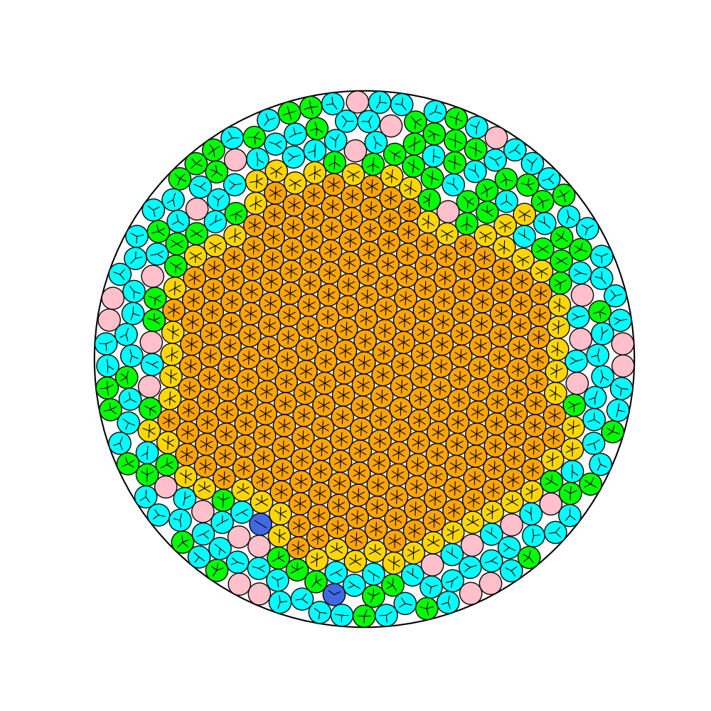
(a)

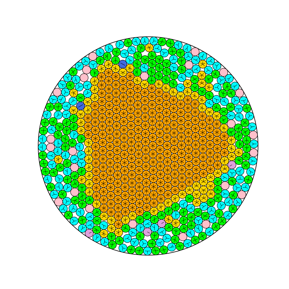
(b)

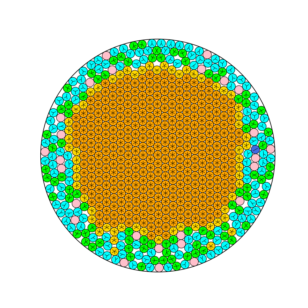
(c)

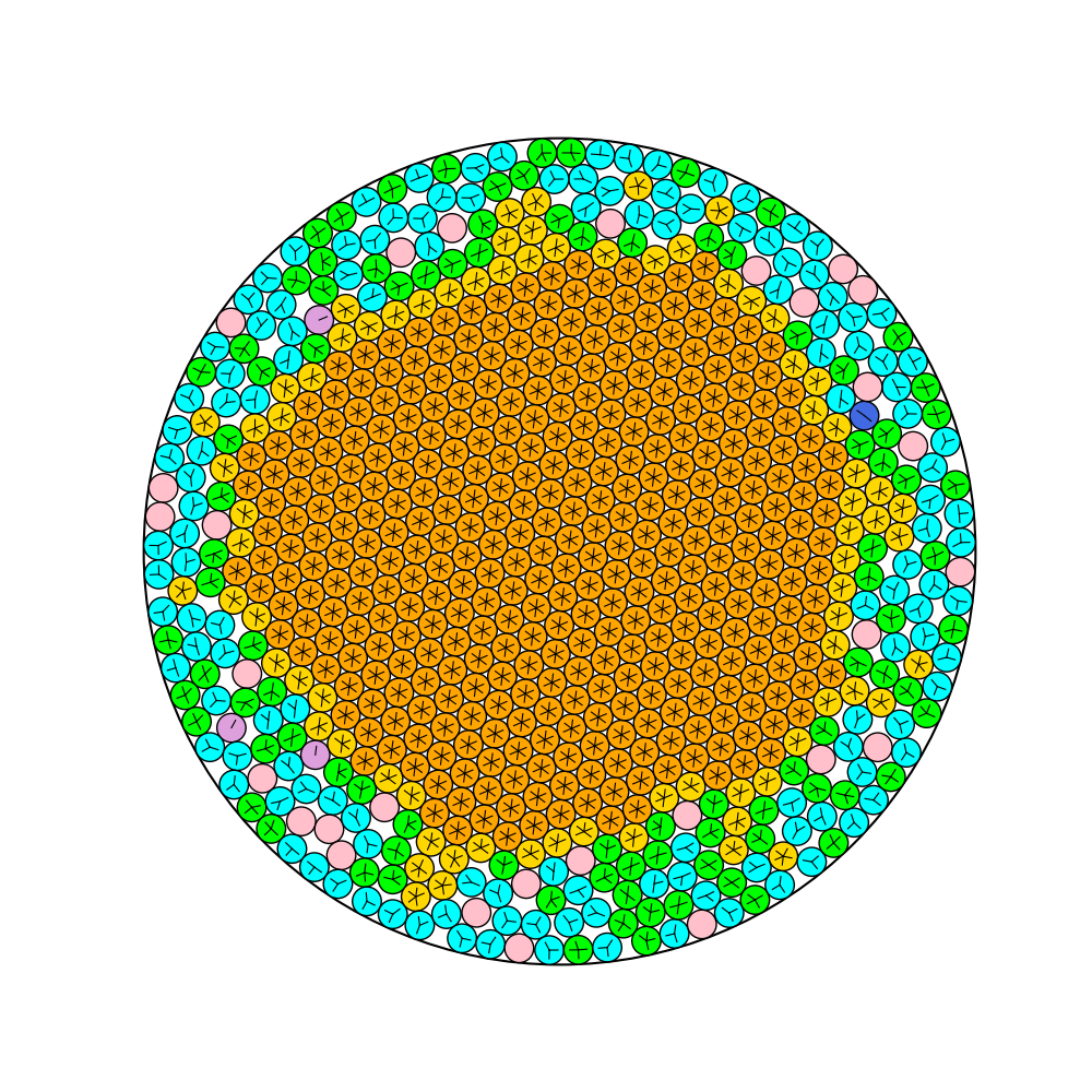
(d)

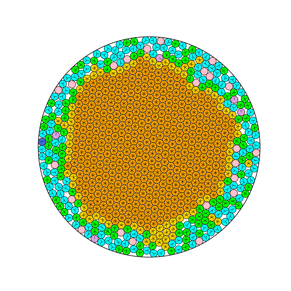
(e)

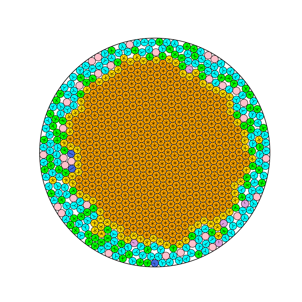
(f)

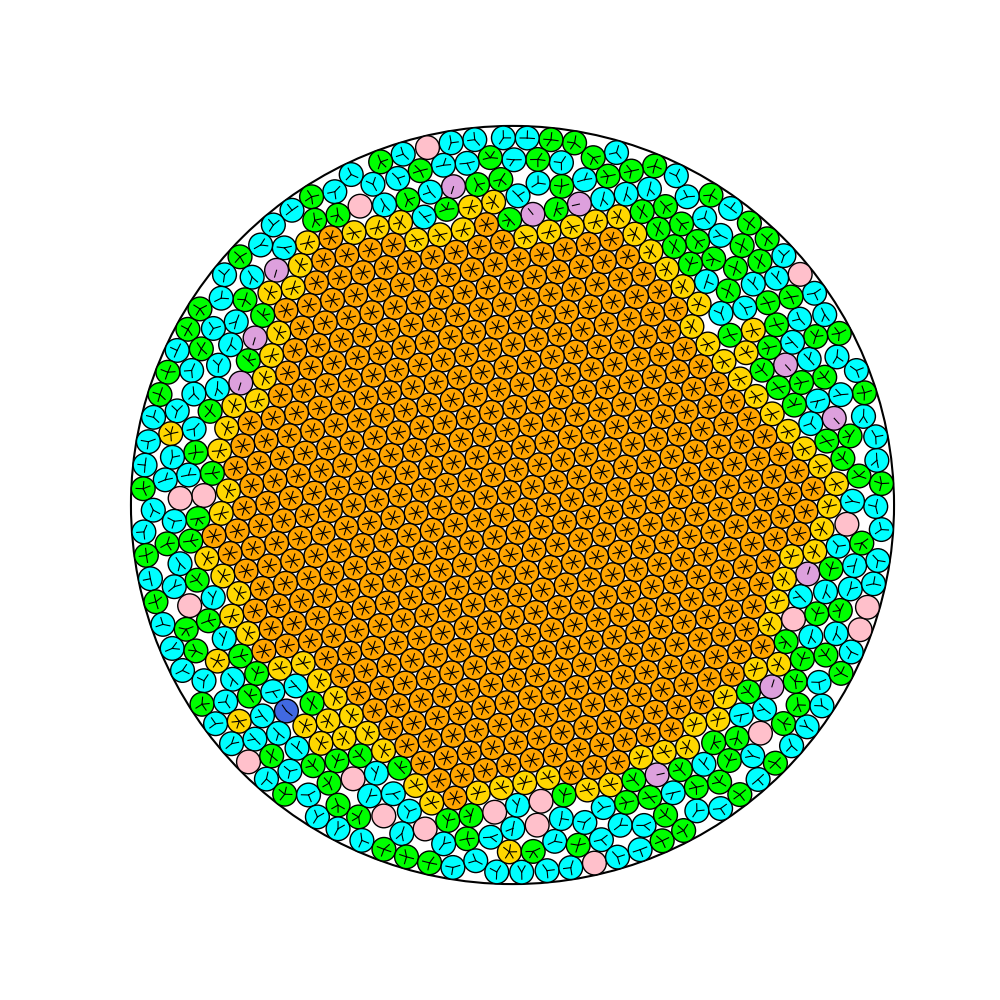
(g)

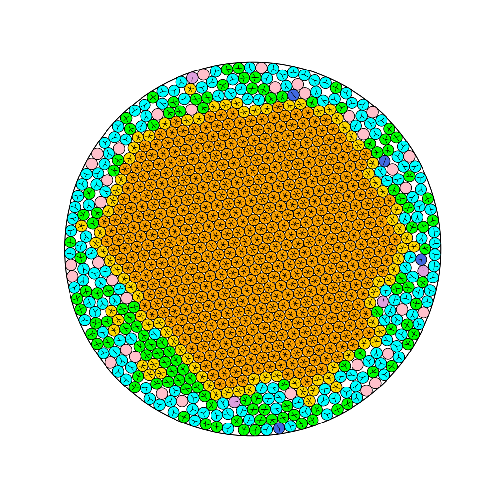
(h)

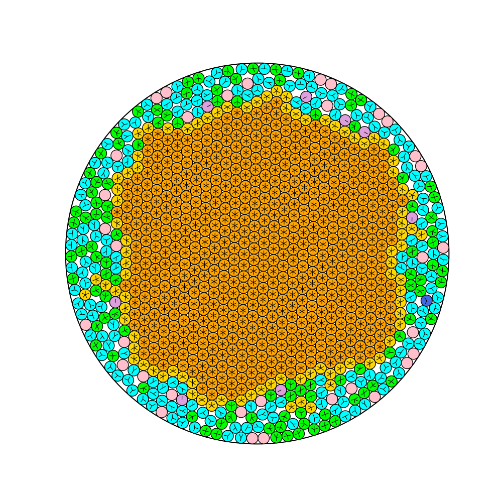
(i)

Figure 5: New improved solutions found by our algorithm for some representative instances on the large scale instances, which have the closest packing in the central zone.

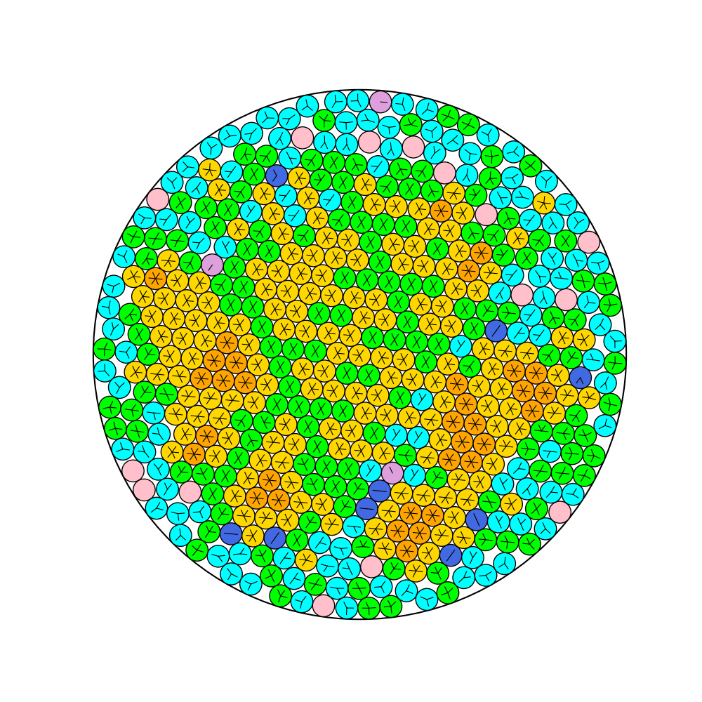
(a)

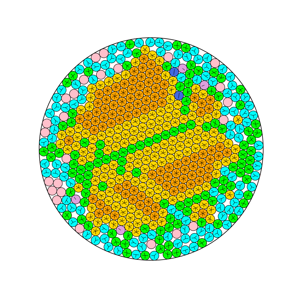
(b)

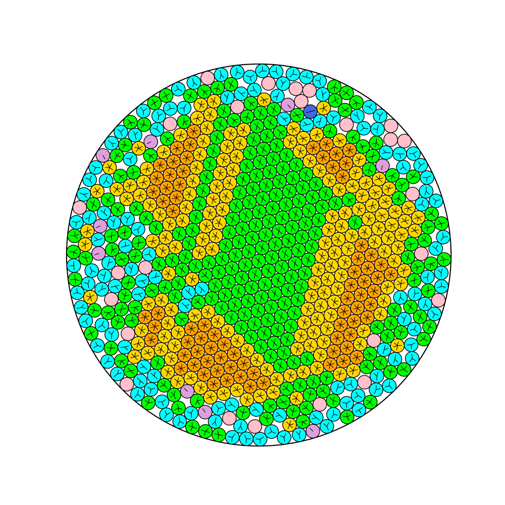
(c)

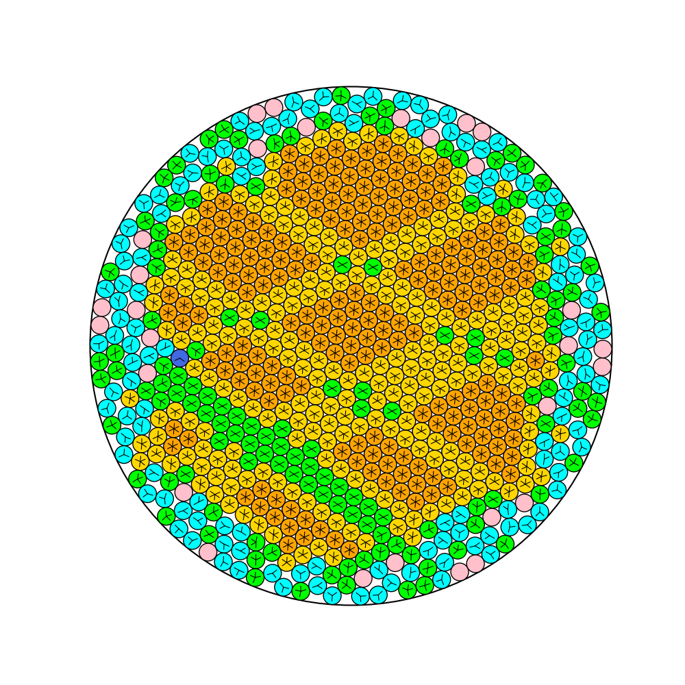
(d)

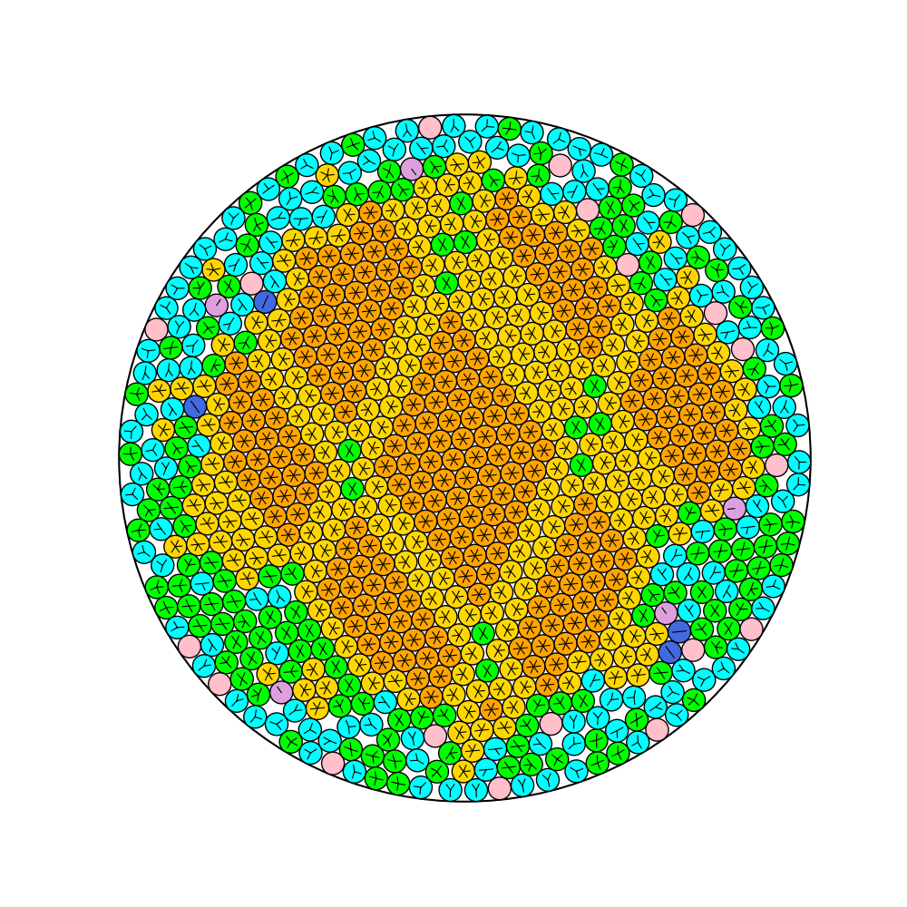
(e)

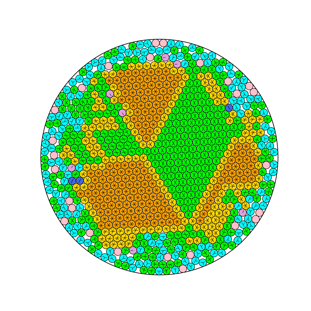
(f)

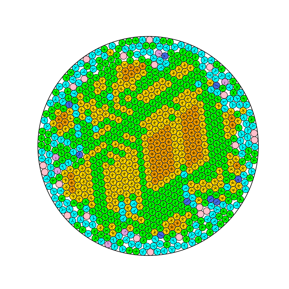
(g)

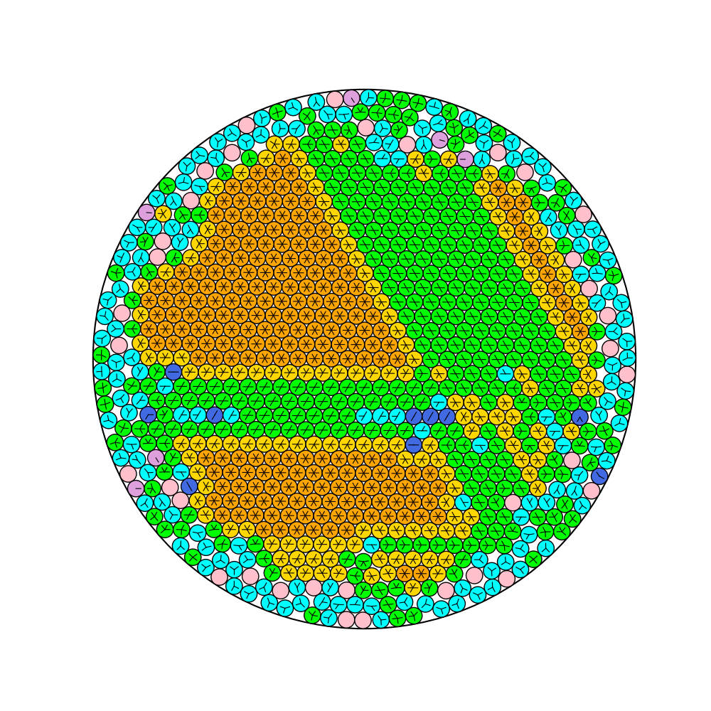
(h)

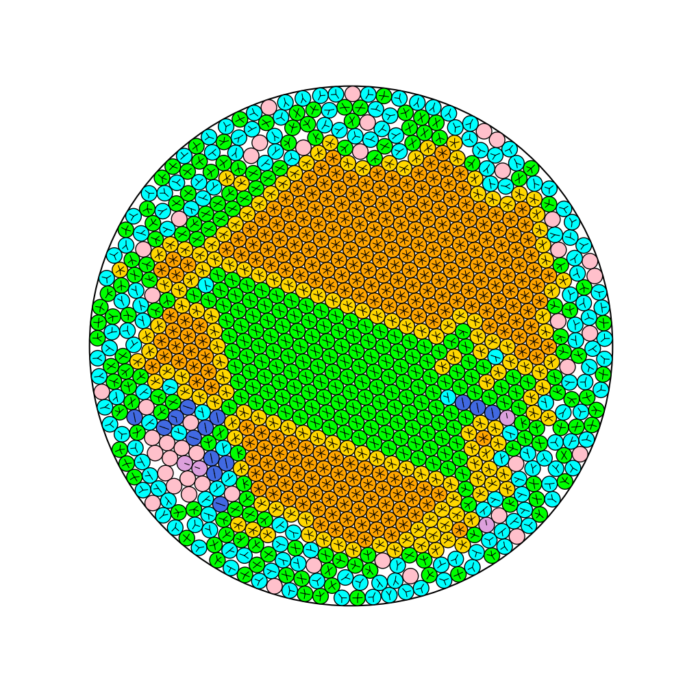
(i)

Figure 6: New improved solutions found by our algorithm for some representative instances on the large scale instances, which do not have the closest packing in the central zone.

6.4 Comparison of GBO (Multi-Batch) and Non-Batch

Table 4: Comparison between 1-batch GBO and 5-batch GBO on the 20 selected large scale instances. The best results of $R_{best}^{\prime}$ and $R_{best}$ and the best results of $R_{avg}^{\prime}$ and $R_{avg}$ appear in bold.

$n$		SED (1-batch GBO)						SED (5-batch GBO)
		$R_{best}^{\prime}$		$R_{avg}^{\prime}$		$time\leavevmode\nobreak\ (s)$		$R_{best}$		$R_{avg}$		$time\leavevmode\nobreak\ (s)$		$R_{best}-R_{best}^{\prime}$		$R_{avg}-R_{avg}^{\prime}$
510		24.4854461416		24.5081091304		48297		24.4210537570		24.4249135890		60259		-6.44E-02		-8.32E-02
610		26.6992073479		26.7150332110		58763		26.6227736610		26.6256150993		55976		-7.64E-02		-8.94E-02
700		28.5679045373		28.5899851016		52511		28.4839888638		28.4877680865		59161		-8.39E-02		-1.02E-01
740		29.2443717879		29.2477209407		56338		29.2418887324		29.2440743866		61698		-2.48E-03		-3.65E-03
760		29.7452134712		29.7964289470		37391		29.6529205123		29.6626249312		45894		-9.23E-02		-1.34E-01
780		30.1284909797		30.1454731784		36161		30.0138757407		30.0164282850		59540		-1.15E-01		-1.29E-01
820		30.8413365443		30.8831339363		87278		30.7489836784		30.7533477503		125921		-9.24E-02		-1.30E-01
890		32.1297407398		32.1758794016		80371		32.0438440391		32.0485774225		88801		-8.59E-02		-1.27E-01
930		32.8196370611		32.8494260033		104544		32.6957714244		32.7024754370		119341		-1.24E-01		-1.47E-01
960		33.3779501763		33.4204902518		100149		33.2554924317		33.2639325269		111880		-1.22E-01		-1.57E-01
513		24.4833011422		24.4880257346		69720		24.4803487672		24.4836476996		53628		-2.95E-03		-4.38E-03
568		25.6742746832		25.6750224839		58749		25.6742746832		25.6747142118		63844		0.00E+00		-3.08E-04
608		26.5872589451		26.5914219805		63320		26.5828030363		26.5852665616		73642		-4.46E-03		-6.16E-03
678		28.0507101923		28.0533386356		49399		28.0452214253		28.0486293696		70367		-5.49E-03		-4.71E-03
737		29.2746711273		29.3098829156		46403		29.1805602263		29.1837249288		59552		-9.41E-02		-1.26E-01
774		29.9122799819		29.9166270797		46759		29.9123498351		29.9157783799		44943		6.99E-05		-8.49E-04
846		31.2194588931		31.2658324893		96767		31.2169756294		31.2320033828		77582		-2.48E-03		-3.38E-02
877		31.7991261202		31.8019948228		105985		31.7939196678		31.7991773790		123868		-5.21E-03		-2.82E-03
923		32.5978399965		32.6013970912		128923		32.5891329001		32.5927036033		117298		-8.71E-03		-8.69E-03
964		33.3301336049		33.3336095372		110927		33.3204312890		33.3287459497		115451		-9.70E-03		-4.86E-03

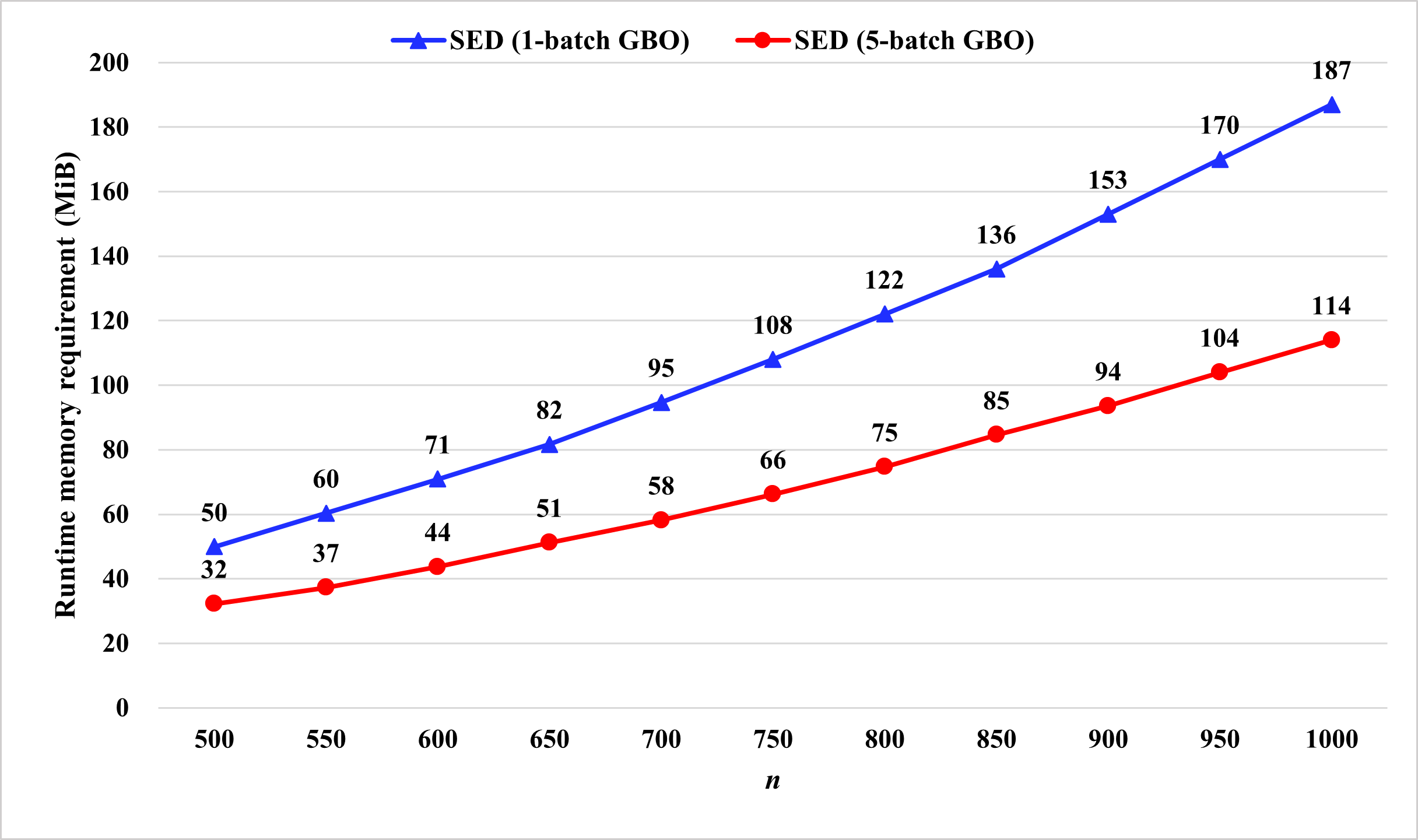
Figure 7: Comparison of the runtime resident memory requirement of SED (5-batch GBO) and SED (1-batch GBO) for the instances $n=$ 500, 550, 600, …, 1000, where the memory requirement is presented in MiB (i.e., MebiByte).

We further do a comparison to evaluate the performance of our proposed GBO module on the large scale instances. We randomly select 10 regular numbers and 10 irregular numbers for the large scale instances, then we perform SED (5-batch GBO) and its variant SED (1-batch GBO), which only changes the batch number from $k=5$ to $k=1$ for SED (5-batch GBO), on the 20 selected instances. Both algorithms run 10 times on each instance independently. The results are shown in Table 4. Note that the 1-batch (non-batch) GBO degenerates to the classic BFGS optimization method.

In the table, we show $n$ for the number of instances, $R_{best}^{\prime}$ and $R_{avg}^{\prime}$ for the best results and average results of 10 runs of SED (1-batch GBO) respectively, $R_{best}$ and $R_{avg}$ for the best results and average results of 10 runs of SED (5-batch GBO) respectively, $time\leavevmode\nobreak\ (s)$ for the average time of obtaining a best solution. $R_{best}-R_{best}^{\prime}$ and $R_{avg}-R_{avg}^{\prime}$ show the difference between two types of results represented where a negative value indicates SED (5-batch GBO) yields better results than SED (1-batch GBO).

From the results, we can observe that SED (5-batch GBO) has 18 best results better than SED (1-batch GBO), 1 best result equal to the latter and 1 best result worse. All the average results of SED (5-batch GBO) are better than SED (1-batch GBO). It clearly demonstrates that the multi-batch method outperforms the non-batch method on large scale instances, and our proposed GBO method has excellent performance on large scale instances.

We also do a comparison of the runtime memory requirement of 5-batch GBO compared and non-batch (i.e., 1-batch). We perform SED (5-batch GBO) and SED (1-batch GBO) for the instances $n=$ 500, 550, 600, …, 1000, and we record the resident memory requirement during the two programs’ runtime. The comparisonal results are presented in Figure 7.

From the Figure 7, we observe that SED (5-batch GBO) requires lower resident runtime memory than SED (1-batch GBO). In particular, 5-batch GBO only needs 60.96% to 64.00% runtime memory of 1-batch GBO (i.e., the classic BFGS) for the instances $n=$ 500, 550, 600, …, 1000. The memory ratio of 5-batch GBO to 1-batch GBO decreases as $n$ increases. It demonstrates multi-batch GBO has advantage of the runtime memory requirement on large scale instances.

6.5 Parameter Study

Three parameters need to be tuned in our proposed algorithm, i.e., the batch strategy of the GBO partition (Section 4.1), the batch number $k$ of GBO (Section 4.1) and the iteration step $S_{iter}$ of SED heuristic (Section 5.2). In this subsection, we give the experimental design and comparisonal results to determine a suitable parameter setting.

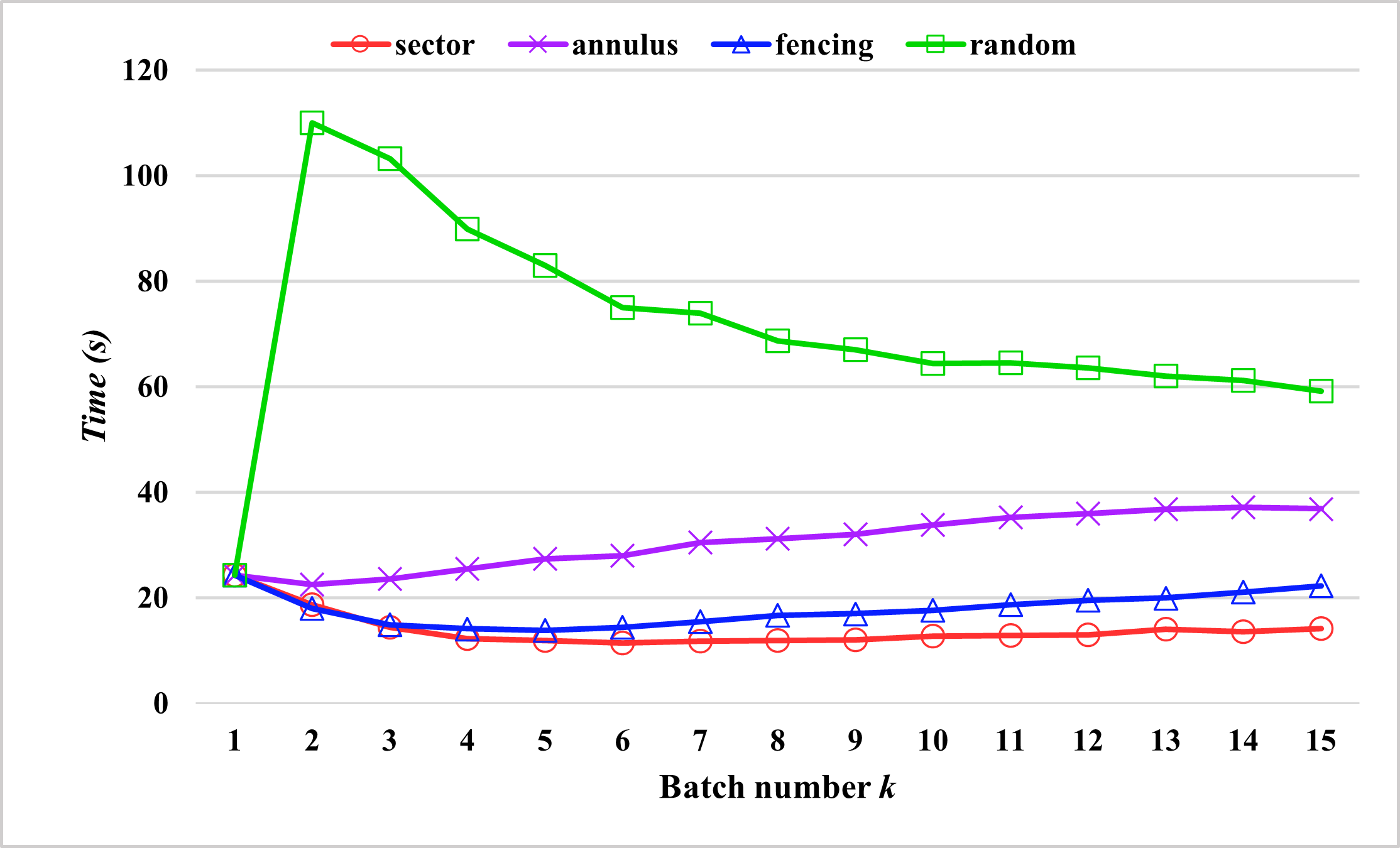
(a)

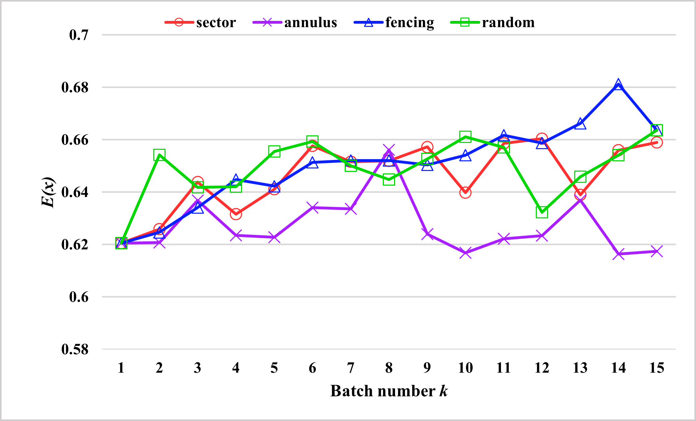
(b)

Figure 8: Comparison between the four partitions of the GBO method on large scale instances.

On batch partition strategy. Since GBO is a continuous optimization method, it is not sensitive to a specific instance, but it is sensitive to the instance scale. Therefore, we performed the four batch partition strategies (sector, annulus, fence and random) on the $n=1000$ scale for the batch number from $k=1$ to $15$, for investigating the performance of the partition strategies on large scale instances. We run each of the settings independently for 1,000 times where each of the runs starts from a random initial layout and terminates at the energy be converged or the maximal iteration step be reached (see in Algorithm 1), and the experimental results of the average time cost and the average converged energy are shown in Figure 8. Note that the GBO method degenerates to the classic BFGS method when the batch number $k=1$ (i.e., the non-batch method).

Figure 8a illustrates the comparison of the average time cost of the four partitions where the X-axis indicates the batch number $k$ and the Y-axis indicates the average time cost of 1,000 runs. From the figure we can observe that:

• The time cost of random partition is significantly higher than non-batch (i.e., $k=1$), which implies applying the random partition on GBO makes the performance worse. Still, the average time cost of the random partition can be decreased as the batch number increases.

• The three geometric batch partition strategies show a similar trend that the average time cost of the three strategies first decreases and then increases with the increasing batch number. The time cost of the annulus partition is slightly lower than non-batch when $k=2$ and $3$, and it is higher than non-batch when $k\geq 4$, the time cost of the sector and fence partitions are all lower than non-batch when $k\geq 2$, and the sector partition has the best performance on the large scale.

• By comparing the random partition with the sector, annulus and fence partitions, we see that a reasonable geometric partition strategy is necessary for solving the PECC problem instead of using the random partition, and the partition strategy directly impacts the performance of the GBO method.

Figure 8b gives the comparison of the average converged energy of the four partitions where the X-axis indicates the batch number $k$ and the Y-axis indicates the average converged energy $E(\boldsymbol{x})$ of 1,000 runs. From the figure we can observe that the four average converged energies of most of the batch partition settings are slightly higher than non-batch. However, most of these average converged energies locate between $0.62$ and $0.66$, and we consider the difference as the experimental error because the difference between these average converged energies compared with non-batch does not exceed 7%.

According to the above discussion, the sector partition of the GBO method can obviously boost the convergence speed, and there is no essential difference between sector partition and non-batch in the convergence result. Therefore, we select the sector partition as the optimal setting of the batch strategy.

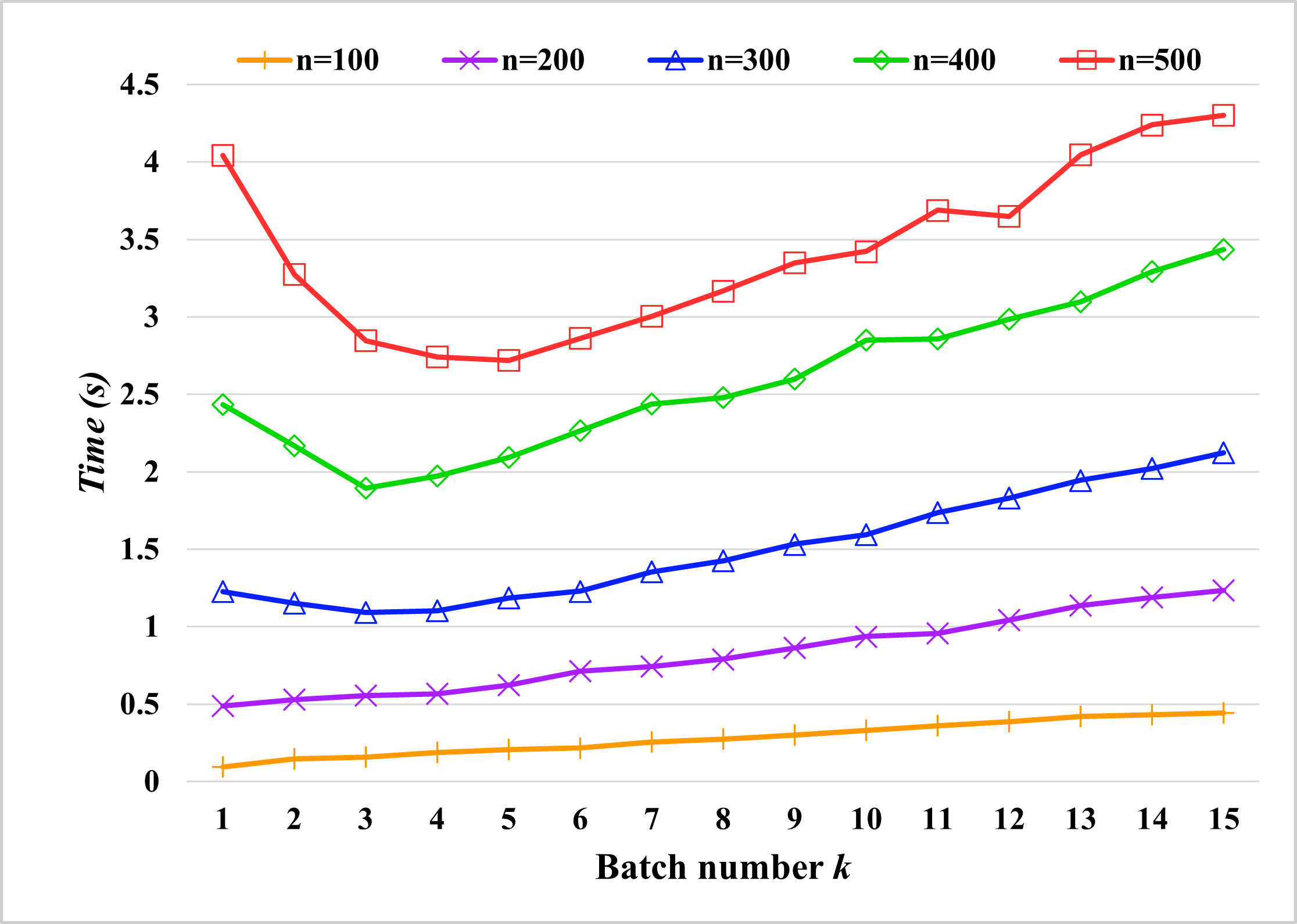
(a)

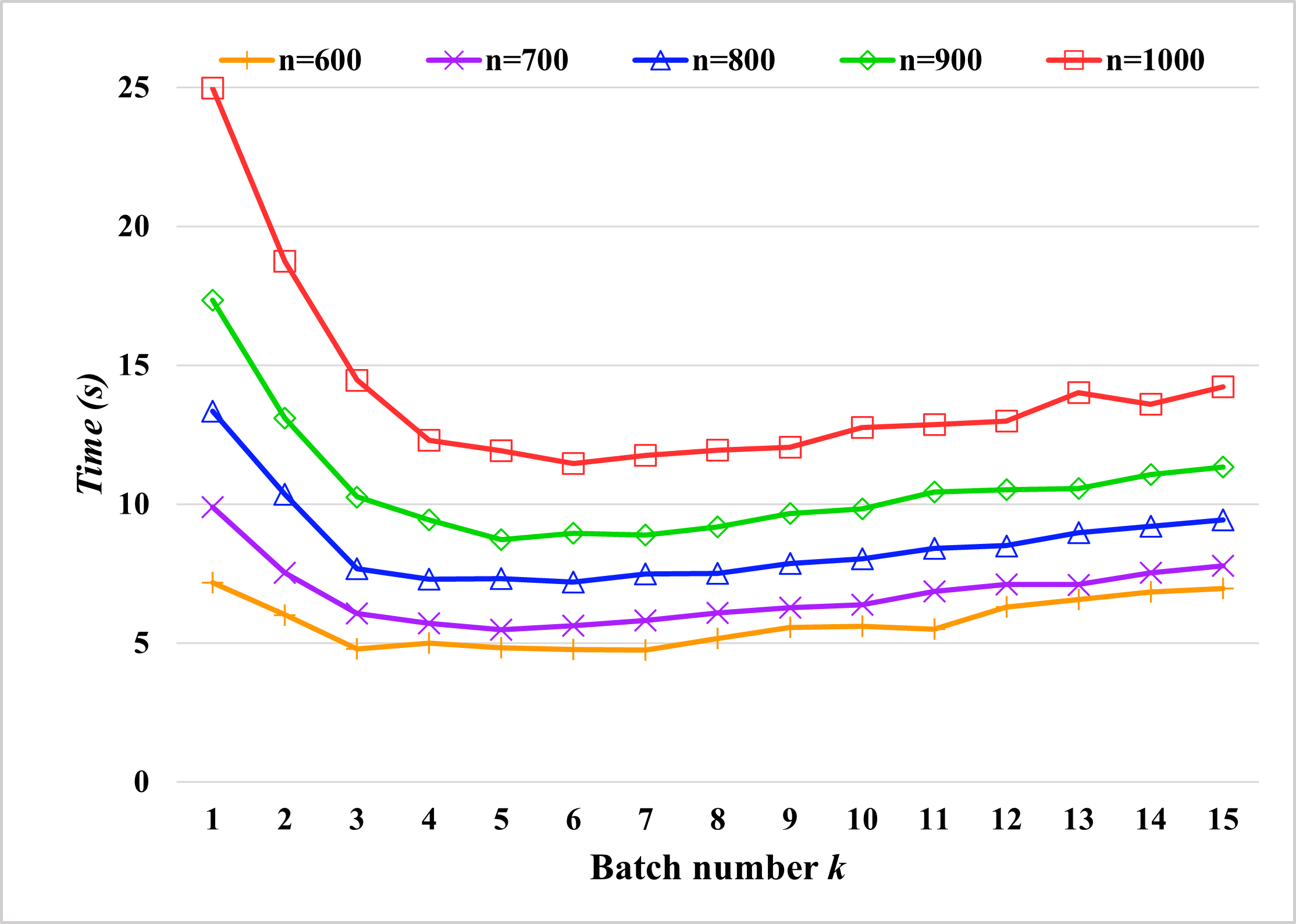
(b)

Figure 9: Comparison between the different settings on the batch number of the GBO method on different scale instances.

Table 5: The optimal batch number settings of GBO for $n=100,200,...,1000$ compared with the non-batch setting.

$n$		$T_{non.}\leavevmode\nobreak\ (s)$		$opt.$		$T_{opt.}\leavevmode\nobreak\ (s)$		Ratio(%)				$n$		$T_{non.}\leavevmode\nobreak\ (s)$		$opt.$		$T_{opt.}\leavevmode\nobreak\ (s)$		Ratio(%)
100		0.09		$k=1$		0.09		100.00%				600		7.17		$k=7$		4.74		66.16%
200		0.49		$k=1$		0.49		100.00%				700		9.90		$k=5$		5.48		55.32%
300		1.23		$k=3$		1.09		88.91%				800		13.35		$k=6$		7.19		53.81%
400		2.43		$k=3$		1.89		77.78%				900		17.35		$k=5$		8.73		50.33%
500		4.04		$k=5$		2.72		67.26%				1000		24.97		$k=6$		11.46		45.89%

On the batch number for various instance scales. To evaluate the performance of GBO on instances of different scales, we perform the GBO method with sector partition on the scale $n=100,200,...,1000$ for the batch number from $k=1$ to $k=15$. We run each of the settings independently 1,000 times where each of the runs starts from a random initial layout and terminates at the energy being converged or the maximal iteration step is reached. The experimental results of the average time cost are shown in Figure 9. Note that the GBO method degenerates to the classic BFGS method when the batch number $k$ is set to 1.

Figures 9a and  9b give the average time cost of the scale $n=100,200,...,500$ and the scale $n=600,700,...,1000$, respectively. The X-axis indicates the batch number $k$ and the Y-axis indicates the average time cost of 1,000 runs. Table 5 shows the comparison of the average time cost of the non-batch and optimal batch setting where the first column of the table gives $n$ of the instances, $T_{non.}$ and $T_{opt.}$ for the average time costs of the non-batch (i.e., $k=1$) and the optimal batch setting, $opt.$ for the optimal setting of the batch number $k$ and Ratio (%) $=\frac{T_{opt.}}{T_{non.}}$ for the average time cost ratio of the optimal batch to non-batch.

From the two Figures 9a and 9b, and Table 5, we have the following observations:

• The curves of the scale for $n=100$ and $n=200$ show that GBO does not work well on very small instances, applying the batch method will increase the convergence time, and GBO needs more time to obtain a converged solution as the batch number increases.

• The curve of the scale for $n=300$ shows that GBO has a small advantage over the non-batch method on moderate scale instances. The average time costs of $k=2,3,4$ and $5$ are slightly lower than non-batch (i.e., $k=1$). The curves of the scale $400\leq n\leq 1000$ show that GBO can reduce the convergence time and boosts the convergence process significantly with a proper batch number setting. And the column of Ratio (%) of the table shows that the ratio will be reduced with the increasing scale, which indicates that GBO has more advantage of accelerating effect as the instance scale increases. The experimental results demonstrate that GBO has excellent performance on large scale instances.

• The curves for the large scale instances, $500\leq n\leq 1000$, show that the average time cost is increasing for batch number $k\geq 8$. It indicates that the batch number is not always better for larger values. And the optimal batch number $k$ of the large scale instances is located in interval $[5,7]$.

According to the above discussion, we use the batch number $k=3$ as the optimal setting for the moderate scale instances, $300\leq n\leq 320$, and the batch number $k=5$ as the trade-off setting for the large scale instances, $500\leq n\leq 1000$.

Table 6: Computational results and comparison of the parameter $S_{iter}$ on the average result ($R_{avg}$) for 12 selected instances where the best results obtained among the tested parameter values are presented in bold.

		$R_{avg}$
$n$  /  $S_{iter}$		100		200		300		400		500		600
305		19.0029499894		19.0022928525		19.0023365854		19.0022767126		19.0027346869		19.0026950563
316		19.3350583426		19.3348928193		19.3352210818		19.3347673471		19.3345842813		19.3346305894
513		24.4871818937		24.4850574870		24.4858380045		24.4843239209		24.4836476996		24.4850158014
568		25.6753984748		25.6746996472		25.6746268914		25.6749397842		25.6747142118		25.6746092173
608		26.5878240724		26.5866285288		26.5860789992		26.5865544926		26.5852665616		26.5867207111
678		28.0509853708		28.0507532028		28.0503173118		28.0509759006		28.0486293696		28.0498132121
740		29.2459673340		29.2469306141		29.2451838453		29.2451220192		29.2440743866		29.2458209932
774		29.9177876254		29.9143968413		29.9117005742		29.9143441746		29.9157783799		29.9153122016
846		31.2425443239		31.2333675583		31.2304459481		31.2320033828		31.2275469287		31.2261977327
877		31.8025272145		31.7999463301		31.8016759748		31.7975804456		31.7991773790		31.7998976078
923		32.5975528505		32.5942894739		32.5935176512		32.5949283036		32.5927036033		32.5947280012
964		33.3335745251		33.3300879802		33.3314171856		33.3271953322		33.3287459497		33.3265773865
Average		27.6066126681		27.6044452780		27.6040300044		27.6037509847		27.6031336198		27.6035015425

On iteration step of SED. The rest of the parameters to be analyzed is the iteration step of SED. We perform SED (5-batch GBO) with the several iteration steps $S_{iter}=100,200,...,600$ on the 12 instances, including 2, 6 and 4 randomly selected instances from the moderate scale, the large scale I and II respectively. The comparison of the iteration steps is shown in Table 6. $n$ is the number of items in the instances, and columns 2 to 7 show the average results, $R_{avg}$, of 10 or 20 runs (20 for the moderate scale and 10 for the large scale) for each tested iteration step $S_{iter}$, and the row of “Average” in the bottom shows the average value of the 12 instance results for each column.

Table 6 shows that the algorithm with $S_{iter}=500$ obtains the best performance in terms of $R_{avg}$ for 6 out of the tested 12 instances, a much higher number than the other 5 tested iteration steps. It has also obtained the best average value of the 12 instance results among the 6 tested iteration steps. As a result, we set the default value of $S_{iter}$ to $500$.

7 Conclusions

In this paper, we aim to address the most representative packing problem, the packing equal circles in a circle problem, on large scale. We propose a novel geometric batch optimization method that not only can significantly speed up the continuous optimization process but also can reduce the memory requirement for finding a local minimum packing configuration. We also propose a solution-space exploring and descent search heuristic accordingly for the search to find a global minimum for the optimization of the overall packing. Besides, we propose an adaptive neighbor object maintenance method, which handles some issues of the existing methods for maintaining the neighbor structure, and it is suitable for dynamic packing problems and online packing problems. Extensive experiments on 21 moderate instances ($n=300$ to 320) and 101 sampled large-scale instances ($n=500$ to 1000) demonstrate the effectiveness and efficiency of our proposed methods. Our algorithm could often find new and better packing results than the current best records. In addition, our geometric batch optimization, heuristic search and adaptive maintenance methods are generic and can be used for other optimization problems. In future work, we will extend our methods for solving other packing problems.

References

- Addis et al. (2008) Addis, B., Locatelli, M., Schoen, F., 2008. Disk packing in a square: a new global optimization approach. INFORMS Journal on Computing 20, 516–524.
- Akeb et al. (2010) Akeb, H., Hifi, M., M’Hallah, R., 2010. Adaptive beam search lookahead algorithms for the circular packing problem. International Transactions in Operational Research 17, 553–575.
- Akeb et al. (2009) Akeb, H., Hifi, M., M’Hallah, R., 2009. A beam search algorithm for the circular packing problem. Computers & Operations Research 36, 1513–1528.
- Baldi et al. (2019) Baldi, M.M., Manerba, D., Perboli, G., Tadei, R., 2019. A generalized bin packing problem for parcel delivery in last-mile logistics. European Journal of Operational Research 274, 990–999.
- Birgin and Sobral (2008) Birgin, E.G., Sobral, F., 2008. Minimizing the object dimensions in circle and sphere packing problems. Computers & Operations Research 35, 2357–2375.
- Burke et al. (2006) Burke, E., Hellier, R., Kendall, G., Whitwell, G., 2006. A new bottom-left-fill heuristic algorithm for the two-dimensional irregular packing problem. Operations Research 54, 587–601.
- Carrabs et al. (2014) Carrabs, F., Cerrone, C., Cerulli, R., 2014. A tabu search approach for the circle packing problem, in: 17th International Conference on Network-Based Information Systems, IEEE. pp. 165–171.
- Castillo et al. (2008) Castillo, I., Kampas, F.J., Pintér, J.D., 2008. Solving circle packing problems by global optimization: numerical results and industrial applications. European Journal of Operational Research 191, 786–802.
- Chen et al. (2018) Chen, M., Tang, X., Song, T., Zeng, Z., Peng, X., Liu, S., 2018. Greedy heuristic algorithm for packing equal circles into a circular container. Computers & Industrial Engineering 119, 114–120.
- Demaine et al. (2010) Demaine, E.D., Fekete, S.P., Lang, R.J., 2010. Circle packing for origami design is hard. arXiv preprint arXiv:1008.1224 .
- Epstein and van Stee (2005) Epstein, L., van Stee, R., 2005. Online square and cube packing. Acta Informatica 41, 595–606.
- Fekete and Hoffmann (2017) Fekete, S.P., Hoffmann, H.F., 2017. Online square-into-square packing. Algorithmica 77, 867–901.
- Fekete et al. (2019) Fekete, S.P., von Höveling, S., Scheffer, C., 2019. Online circle packing, in: Algorithms and Data Structures: 16th International Symposium, WADS 2019, Edmonton, AB, Canada, August 5–7, 2019, Proceedings 16, Springer. pp. 366–379.
- Fodor (1999) Fodor, F., 1999. The densest packing of 19 congruent circles in a circle. Geometriae Dedicata 74, 139–145.
- Fodor (2000) Fodor, F., 2000. The densest packing of 12 congruent circles in a circle. Beiträge Algebra Geom 41, 401–409.
- Fodor (2003) Fodor, F., 2003. The densest packing of 13 congruent circles in a circle. Beiträge zur Algebra und Geometrie 44, 431–440.
- Goldberg (1971) Goldberg, M., 1971. Packing of 14, 16, 17 and 20 circles in a circle. Mathematics Magazine 44, 134–139.
- Görtler et al. (2017) Görtler, J., Schulz, C., Weiskopf, D., Deussen, O., 2017. Bubble treemaps for uncertainty visualization. IEEE Transactions on Visualization and Computer Graphics 24, 719–728.
- Graham and Peck (1968) Graham, R., Peck, C., 1968. Sets of points with given maximum separation (problem e1921). The American Mathematical Monthly 75, 80–81.
- Graham et al. (1998) Graham, R.L., Lubachevsky, B.D., Nurmela, K.J., Östergård, P.R., 1998. Dense packings of congruent circles in a circle. Discrete Mathematics 181, 139–154.
- Grosso et al. (2010) Grosso, A., Jamali, A., Locatelli, M., Schoen, F., 2010. Solving the problem of packing equal and unequal circles in a circular container. Journal of Global Optimization 47, 63–81.
- Hartman et al. (2019) Hartman, T., Mazáč, D., Rastelli, L., 2019. Sphere packing and quantum gravity. Journal of High Energy Physics 2019, 1–68.
- He et al. (2013) He, K., Mo, D., Ye, T., Huang, W., 2013. A coarse-to-fine quasi-physical optimization method for solving the circle packing problem with equilibrium constraints. Computers & Industrial Engineering 66, 1049–1060.
- He et al. (2021) He, K., Tole, K., Ni, F., Yuan, Y., Liao, L., 2021. Adaptive large neighborhood search for solving the circle bin packing problem. Computers & Operations Research 127, 105140.
- He et al. (2018) He, K., Ye, H., Wang, Z., Liu, J., 2018. An efficient quasi-physical quasi-human algorithm for packing equal circles in a circular container. Computers & Operations Research 92, 26–36.
- Hifi and M’Hallah (2004) Hifi, M., M’Hallah, R., 2004. Approximate algorithms for constrained circular cutting problems. Computers & Operations Research 31, 675–694.
- Hifi and M’Hallah (2007) Hifi, M., M’Hallah, R., 2007. A dynamic adaptive local search algorithm for the circular packing problem. European Journal of Operational Research 183, 1280–1294.
- Hifi et al. (2004) Hifi, M., Paschos, V.T., Zissimopoulos, V., 2004. A simulated annealing approach for the circular cutting problem. European Journal of Operational Research 159, 430–448.
- Hifi and Yousef (2019) Hifi, M., Yousef, L., 2019. A local search-based method for sphere packing problems. European Journal of Operational Research 274, 482–500.
- Hokama et al. (2016) Hokama, P., Miyazawa, F.K., Schouery, R.C., 2016. A bounded space algorithm for online circle packing. Information Processing Letters 116, 337–342.
- Huang et al. (2005) Huang, W., Li, Y., Akeb, H., Li, C., 2005. Greedy algorithms for packing unequal circles into a rectangular container. Journal of the Operational Research Society 56, 539–548.
- Huang and Xu (1999) Huang, W., Xu, R., 1999. Two personification strategies for solving circles packing problem. Science in China Series E: Technological Sciences 42, 595–602.
- Huang and Ye (2011) Huang, W., Ye, T., 2011. Global optimization method for finding dense packings of equal circles in a circle. European Journal of Operational Research 210, 474–481.
- Huang et al. (2003) Huang, W.Q., Li, Y., Jurkowiak, B., Li, C.M., Xu, R.C., 2003. A two-level search strategy for packing unequal circles into a circle container, in: International Conference on Principles and Practice of Constraint Programming, Springer. pp. 868–872.
- Huang et al. (2006) Huang, W.Q., Li, Y., Li, C.M., Xu, R.C., 2006. New heuristics for packing unequal circles into a circular container. Computers & Operations Research 33, 2125–2142.
- Kravitz (1967) Kravitz, S., 1967. Packing cylinders into cylindrical containers. Mathematics Magazine 40, 65–71.
- Lai et al. (2022) Lai, X., Hao, J.K., Yue, D., Lü, Z., Fu, Z.H., 2022. Iterated dynamic thresholding search for packing equal circles into a circular container. European Journal of Operational Research 299, 137–153.
- Leao et al. (2020) Leao, A.A., Toledo, F.M., Oliveira, J.F., Carravilla, M.A., Alvarez-Valdés, R., 2020. Irregular packing problems: A review of mathematical models. European Journal of Operational Research 282, 803–822.
- Leung et al. (1990) Leung, J.Y., Tam, T.W., Wong, C.S., Young, G.H., Chin, F.Y., 1990. Packing squares into a square. Journal of Parallel and Distributed Computing 10, 271–275.
- Lintzmayer et al. (2019) Lintzmayer, C.N., Miyazawa, F.K., Xavier, E.C., 2019. Online circle and sphere packing. Theoretical Computer Science 776, 75–94.
- Liu et al. (2016) Liu, J., Zhang, K., Yao, Y., Xue, Y., Guan, T., 2016. A heuristic quasi-physical algorithm with coarse and fine adjustment for multi-objective weighted circles packing problem. Computers & Industrial Engineering 101, 416–426.
- López and Beasley (2011) López, C.O., Beasley, J.E., 2011. A heuristic for the circle packing problem with a variety of containers. European Journal of Operational Research 214, 512–525.
- Lü and Huang (2008) Lü, Z., Huang, W., 2008. Perm for solving circle packing problem. Computers & Operations Research 35, 1742–1755.
- Martello et al. (2003) Martello, S., Monaci, M., Vigo, D., 2003. An exact approach to the strip-packing problem. INFORMS Journal on Computing 15, 310–319.
- Melissen (1994) Melissen, H., 1994. Densest packings of eleven congruent circles in a circle. Geometriae Dedicata 50, 15–25.
- Miyazawa and Wakabayashi (2003) Miyazawa, F.K., Wakabayashi, Y., 2003. Cube packing. Theoretical Computer Science 297, 355–366.
- Mladenović et al. (2005) Mladenović, N., Plastria, F., Urošević, D., 2005. Reformulation descent applied to circle packing problems. Computers & Operations Research 32, 2419–2434.
- Murakami et al. (2015) Murakami, H., Higo, Y., Kusumoto, S., 2015. Clonepacker: A tool for clone set visualization, in: IEEE 22nd International Conference on Software Analysis, Evolution, and Reengineering (SANER), IEEE. pp. 474–478.
- Nurmela and Östergård (1997) Nurmela, K.J., Östergård, P.R., 1997. Packing up to 50 equal circles in a square. Discrete & Computational Geometry 18, 111–120.
- Pirl (1969) Pirl, U., 1969. Der mindestabstand von n in der einheitskreisscheibe gelegenen punkten. Mathematische Nachrichten 40, 111–124.
- Rao et al. (2021) Rao, Y., Wang, P., Luo, Q., 2021. Hybridizing beam search with tabu search for the irregular packing problem. Mathematical Problems in Engineering 2021.
- Reis (1975) Reis, G.E., 1975. Dense packing of equal circles within a circle. Mathematics Magazine 48, 33–37.
- Ren-Pu and Powell (1983) Ren-Pu, G., Powell, M.J., 1983. The convergence of variable metric matrices in unconstrained optimization. Mathematical Programming 27, 123–143.
- Specht (2022) Specht, E., 2022. Packomania website: http://www.packomania.com .
- Stoyan and Yaskov (2014) Stoyan, Y., Yaskov, G., 2014. Packing unequal circles into a strip of minimal length with a jump algorithm. Optimization Letters 8, 949–970.
- Stoyan et al. (2020) Stoyan, Y., Yaskov, G., Romanova, T., Litvinchev, I., Yakovlev, S., Cantú, J.M.V., 2020. Optimized packing multidimensional hyperspheres: a unified approach. Mathematical Biosciences and Engineering 17, 6601–6630.
- Wang et al. (2006) Wang, W., Wang, H., Dai, G., Wang, H., 2006. Visualization of large hierarchical data by circle packing, in: Proceedings of the SIGCHI Conference on Human Factors in Computing Systems, pp. 517–520.
- Wang et al. (2019) Wang, Y., Wang, Y., Sun, J., Huang, C., Zhang, X., 2019. A stimulus–response-based allocation method for the circle packing problem with equilibrium constraints. Physica A: Statistical Mechanics and its Applications 522, 232–247.
- Yanchevskyi et al. (2020) Yanchevskyi, I., Lachmayer, R., Mozgova, I., Lippert, R.B., Yaskov, G., Romanova, T., Litvinchev, I., 2020. Circular packing for support-free structures. EAI Endorsed Transactions on Energy Web 7, e3–e3.
- Zhao et al. (2020) Zhao, C., Jiang, L., Teo, K.L., 2020. A hybrid chaos firefly algorithm for three-dimensional irregular packing problem. Journal of Industrial & Management Optimization 16, 409.
- Zhao et al. (2021) Zhao, H., She, Q., Zhu, C., Yang, Y., Xu, K., 2021. Online 3d bin packing with constrained deep reinforcement learning, in: Proceedings of the AAAI Conference on Artificial Intelligence, pp. 741–749.