Decision Support System for Chronic Diseases Based on Drug-Drug Interactions

Abstract

Many patients with chronic diseases resort to multiple medications to relieve various symptoms, which raises concerns about the safety of multiple medication use, as severe drug-drug antagonism can lead to serious adverse effects or even death. This paper presents a Decision Support System, called DSSDDI, based on drug-drug interactions to support doctors prescribing decisions. DSSDDI contains three modules, Drug-Drug Interaction (DDI) module, Medical Decision (MD) module and Medical Support (MS) module. The DDI module learns safer and more effective drug representations from the drug-drug interactions. To capture the potential causal relationship between DDI and medication use, the MD module considers the representations of patients and drugs as context, DDI and patients’ similarity as treatment, and medication use as outcome to construct counterfactual links for the representation learning. Furthermore, the MS module provides drug candidates to doctors with explanations. Experiments on the chronic data collected from the Hong Kong Chronic Disease Study Project and a public diagnostic data MIMIC-III demonstrate that DSSDDI can be a reliable reference for doctors in terms of safety and efficiency of clinical diagnosis, with significant improvements compared to baseline methods. Source code of the proposed DSSDDI is publicly available at https://github.com/TianBian95/DSSDDI.

I Introduction

Due to physiological changes, increased risk of disease and decreased drug clearance, problematic polypharmacy has become a significant factor in the increased risk of severe Adverse Drug Events (ADEs), hospital admissions, and death in chronic patients [1]. This issue is especially prominent during critical times, such as the epidemic of coronavirus disease (COVID-19). With the shortage of clinical resources, medication for chronic patients lacks guidance from professional doctors and presents unique challenges. Further, polypharmacy increases the potential for drug-drug interactions (DDI), including potentially inappropriate drug combinations present in prescription medications [2], which accelerates the imbalance between the complex needs of the chronic patients and the problems caused by the multiple medications. A systematic approach is required to efficiently support doctors in tailoring of medication regimens to extricate the chronic patients from the dilemma.

Advanced technologies nowadays have been applied to develop more effective decision support systems for better-informed decisions [3]. However, some methods [4, 5] that learn from association between patients and drugs, mainly rely on patient and drug features, but ignore the impact of DDI on medical decisions. Some other methods [6] make use of DDI to learn drug embeddings but fail to capture the causal relationship between drug embeddings and medication suggestions. Therefore, our goal in this paper is: (1) leveraging DDI to avoid severe ADEs in medication suggestions, and (2) employing the causal model [7, 8] to learn the potential causal relationships between DDI and medication suggestions to improve the accuracy.

We studied the chronic patients through the Hong Kong Chronic Disease Study Project, including their personal features, clinical history, psychological assessment and medication use. We propose a decision support system, DSSDDI, that can provide explainable medication suggestions for chronic diseases. A bipartite graph can be naturally formed on the patients and drugs, and then DSSDDI applies link prediction on the bipartite graph for medication suggestions. With the help of an external DDI knowledge graph, the decision support system inputs patient features and outputs medication suggestions and the corresponding DDI explanations to doctors as clinical diagnostic references. The design of DSSDDI is depicted in Fig. 1.

Figure 1: Our proposed decision support system uses external knowledge of DDI. Given patient features as input, a doctor can obtain the medication suggestions from the system, as well as the corresponding DDI explanations.

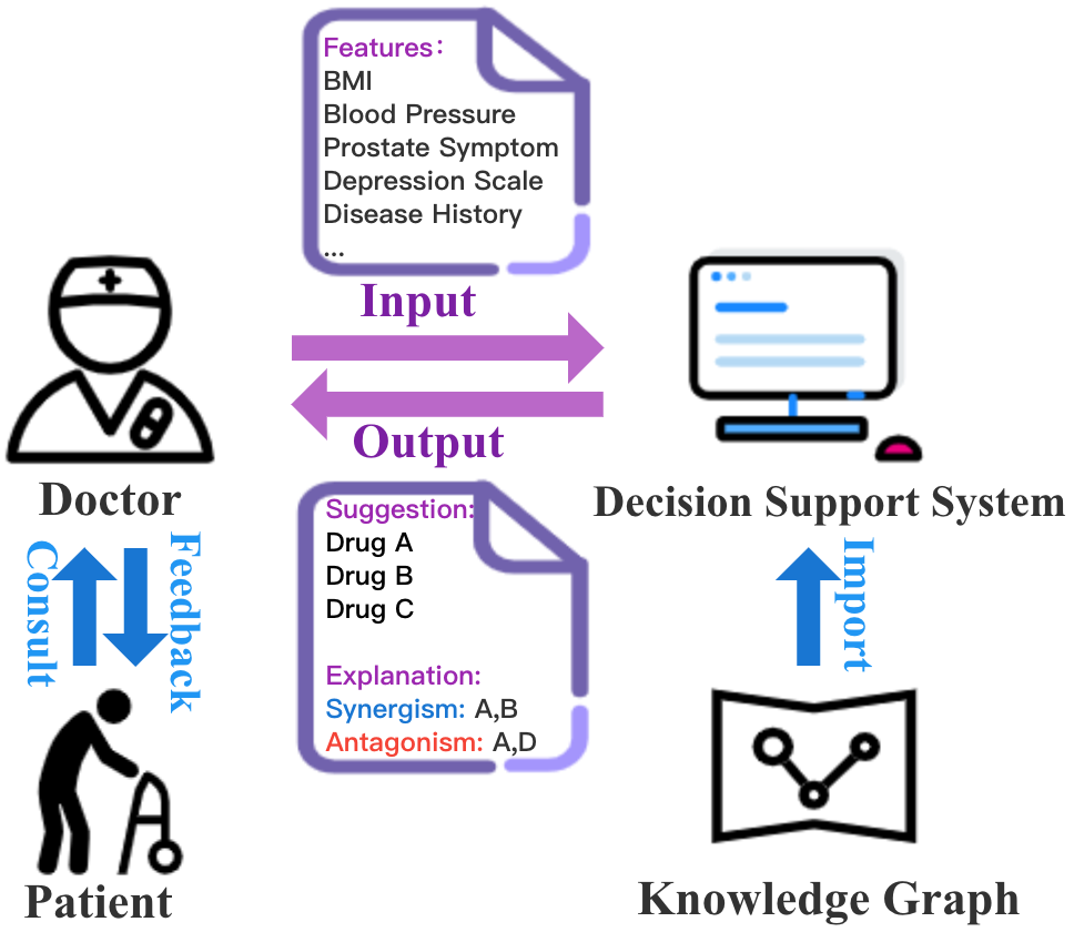
There are three modules in DSSDDI: the Drug-Drug Interaction (DDI) module, the Medical Decision (MD) module and the Medical Support (MS) module. The function and merit of each module are described as follows.

• The DDI module uses our proposed Drug-Drug Interaction Graph Convolutional Network (DDIGCN) to learn drug representations from synergistic or antagonistic effects between drugs. The DDI module can alleviate severe adverse drug events, which is crucial to ensure safe and effective medical decisions.

• The MD module uses a Medical Decision Graph Convolutional Network (MDGCN) to suggest drugs. We construct counterfactual links to augment the training data for MDGCN based on the causal model that considers the representations of patients and drugs as context, DDI and patients’ similarity as treatment, and medication use as outcome. This can learn the causal relationship between DDI and medication use.

• After obtaining the suggested drugs, the MS module extracts coherent subgraphs with DDI knowledge as explainable factors for doctors’ reference. Such subgraphs illustrate the synergistic and antagonistic effects between drugs.

Experiments on data from Hong Kong Chronic Disease Study Project and public diagnostic data MIMIC-III [9] demonstrate the superior performance of DSSDDI in medication suggestion and its explainability.

II Data Collection

Our study focuses on the patients participating in the Hong Kong Chronic Disease Study Project, who may require multiple medications because they have multi-chronic diseases. We collect data from questionnaire interviews and laboratory results to predict what medications they would need to take. Since drug-drug interactions are the primary consideration for doctors when prescribing medications, DSSDDI is designed to avoid the inclusion of drugs that contain antagonistic effects between each other and suggest drugs that have synergistic effects. In this section, we first introduce the participants enrolled in this project, then describe the drugs we use for the decision support system, followed by a further description of the drug-drug interactions used in this paper.

II-A Participants

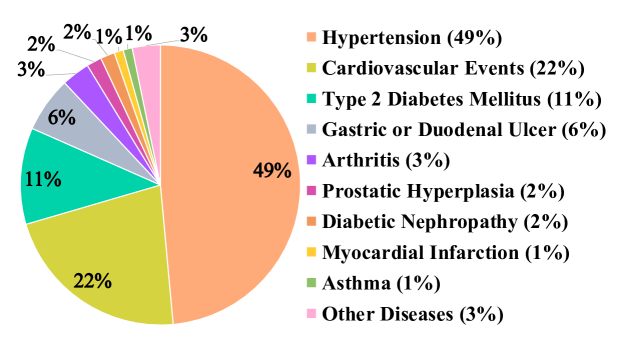
This project was initiated by Prince of Wales Hospital in 2001. Subjects aged 65 years and older were recruited under the project. The cohort was invited for a questionnaire interview and measurement of physical performance for 1 – 4 times during 2001 – 2017. We extracted 2254 male and 1903 female interview records. The distribution of the diseases suffered by these subjects is shown in Fig. 2. Hypertension, cardiovascular diseases, diabetes, digestive diseases and arthritis are the chronic diseases they commonly suffer.

The questionnaire interview contains three types of subject information. The first type is the personal information about the participants such as gender and age. The second type is the clinical history of participants. For example, participants were asked whether they had prostatitis before or had taken taken the Alpha-blocker. It is important to note that the questionnaire only mentions the clinical history of the family of drugs, but not the specific drugs. The third type is a psychological assessment of the participants, including the Geriatric Depression Scale (GDS) Score and some emotional questions, such as whether they had felt downhearted in the last four weeks. The physical examination included the participants’ blood pressure, Body Mass Index (BMI), etc. Combining the three types of information, we collected a total of 71 features.

II-B Medication Use

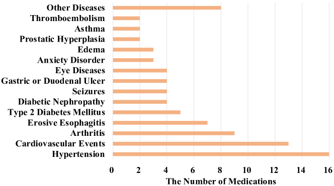
In total, the participants took 86 medications that are commonly used to treat chronic conditions. For example, Doxazosin, a medication commonly used by the participants, is an alpha-1 adrenergic receptor used to treat mild to moderate hypertension and urinary obstruction due to benign prostatic hyperplasia. Fig. 3 shows the distribution of these 86 drugs for various diseases. As there is usually more than one drug available for treating a chronic disease such as diabetes, gastrointestinal diseases, and arthritis, the choice of the most appropriate drug is a significant consideration for doctors, and our proposed DSSDDI is designed to help doctors make decisions more efficiently. We collect pre-trained embedding of each drug in the Drug Repurposing Knowledge Graph (DRKG) [10] as the original feature of the drug for the medication suggestion prediction. Each pre-trained embedding is trained using a classical knowledge representation learning method named TransE [11] with a dimension size of 400.

Figure 2: The proportion of patients with various diseases.

Figure 3: The distribution of medications for common chronic diseases.

II-C Drug-Drug Interactions

DrugCombDB [12] is a database containing drug-drug interactions obtained from various sources, including external databases, manual curations from PubMed literature and experimental results. We take the drug-drug interactions that have been classified as exhibiting synergistic or antagonistic effects from DrugCombDB. For the 86 drugs used for suggestion, we extract 97 drug pairs classified as having synergistic effects and 243 drug pairs classified as having antagonistic effects from the DrugCombDB database. Based on these drug-drug interactions, the proposed decision support system obtains better effectiveness by avoiding pairs with antagonistic effects and promoting pairs with synergistic effects in medication suggestions.

Figure 4: The proposed decision support system (DSSDDI) consists of three modules: DDI module, MD module and MS module. (a) In the DDI module, we construct the drug-drug interaction matrix where the entries of the matrix represent the synergistic effects (blue) or antagonistic effects (red) among drugs. Through a proposed DDIGCN, we obtain drug relation representations shared with the MD module. (b) In the MD module, we first construct a bipartite graph from the medication use (black lines) and counterfactual links (yellow dashed lines). Then, we obtain the suggested drugs through the proposed MDGCN. (c) In the MS module, the explanation of the suggested drugs is extracted through a subgraph querying algorithm.

III Problem Formulation

In this paper, we design three modules for the proposed decision support system: Drug-Drug Interaction (DDI) module, Medical Decision (MD) module and Medical Support (MS) module. In this section, we will first introduce the generalized decision support system, then define the DDI graph constructed in the DDI module, and give the definitions of medical decision and medical support.

Definition 1 (Decision Support System)

Given a set of drug candidates denoted as $V=\{D_{1},D_{2},\cdots,D_{|V|}\}$, the decision support system is designed to suggest a list of appropriate drugs from $V$ to a patient $S_{i}$ based on the patient features $\mathbf{x}_{i}$.

Definition 2 (Drug-Drug Interaction (DDI) Graph)

We define the drug-drug interaction (DDI) graph as $G=(V,E)$, where the node set $V=\{D_{1},D_{2},\cdots,D_{|V|}\}$ denotes the drugs and the edge set $E$ denotes the synergistic or antagonistic effects between drugs. An edge $e_{uv}=1$ in $E$ represents a synergistic effect between drugs $D_{u}$ and $D_{v}$, and an edge $e_{uv}=-1$ in $E$ represents an antagonistic effect.

Definition 3 (Medical Decision)

The target of medical decision is to identify the most effective combination of drugs for the patients from a set of drug candidates. By representing the relationship between patients and drugs as a bipartite graph, we formulate the medical decision problem based on the results of link prediction and further use the drug-drug interactions as constraints to identify the appropriate drugs. Specifically, suppose that we are given a set of observed patients’ data denoted as $\mathcal{O}=\{\mathbf{x}_{i},\mathbf{y}_{i}\}^{m}_{i=1}$, $\mathbf{y}_{i}$ is a vector with $y_{iv}=1$ if patient $S_{i}$ is taking drug $D_{v}$ and $y_{iv}=0$ otherwise, $m$ is the number of observed patients. The set of unobserved patients’ data is denoted as $\mathcal{U}=\{\mathbf{x}_{j},\mathbf{y}_{j}\}^{n}_{j=m+1}$, where $n$ is the number of all patients. Given the patient features ${\mathbf{x}_{j}}$, the target of medical decision is first to predict the score of each drug and then to suggest the most $k$ reliable drugs $Q=\{D_{q1},D_{q2},\cdots,D_{qk}\}$ to the unobserved patient $S_{j}$ based on drug-drug interactions.

Definition 4 (Medical Support)

The target of medical support is to find explainable factors through drug-drug interactions for the $k$ suggested drugs $Q=\{D_{q1},D_{q2},\cdots,D_{qk}\}$. Specifically, given $Q$ and the DDI graph $G$, we can find a subgraph $G_{sub}$ of $G$ containing all drug-drug interactions associated with the suggested drugs, and thus can act as medical support for the Medical Decision module.

IV The Proposed DSSDDI

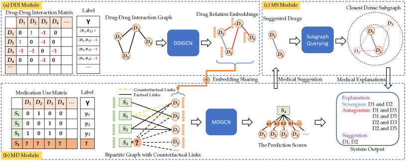
Fig. 4 depicts the overall architecture of DSSDDI which consists of three modules: Drug-Drug Interaction, Medical Decision and Medical Support. In Drug-Drug Interaction, we learn the drug relation representations. In Medical Decision, we capture the causal relationship between DDI and medication use. In Medical Support, we generate the explanation of the suggested drugs. In this section, we elaborate on each module.

IV-A Drug-Drug Interaction Module

In the Drug-Drug Interaction (DDI) module, we first develop a model, DDIGCN, to learn the drug representations. The main idea is to learn drug relation features through synergistic or antagonistic effects between drugs. In the following, we first describe how to construct the DDI graph, then illustrate how to update the drug representations by DDIGCN, and finally describe the model training process.

IV-A1 DDI Graph Construction

As described in Definition 2, we construct the DDI graph $G=(V,E)$ based on the data collected from DrugCombDB [12] with Drug ID embedding vectors $\mathbf{z}_{v}$ for $D_{v}\in V$. To better capture the relation features among drugs, we use one-hot ID embeddings instead of pre-trained embeddings as the original features in this DDI module. Besides synergistic and antagonistic effects, we add the third type of edges between drugs in the DDI graph to explicitly indicate that they have no interactions. Specifically, we randomly sample drug pairs, denoted as $D_{u}$ and $D_{v}$, from $V$ with no synergistic or antagonistic effect, and create an edge $e_{uv}=0$ to represent the lack of interactions between them. In this manner, DDIGCN can capture synergistic and antagonistic drug-drug interactions as well as no interactions in drug embeddings.

IV-A2 DDIGCN

In this step, we design a DDIGCN to update the drug representations. We use Graph Isomorphism Network (GIN) [13] as the backbone. The graph convolutional operation is defined as:

$$\mathbf{z}^{(t)}_{v}=f^{(t)}_{\mathbf{\Theta_{1}}}\left((1+\epsilon^{(t)})\cdot\mathbf{z}^{(t-1)}_{v}+\frac{\sum_{u\in\mathcal{N}_{v}}\mathbf{z}^{(t-1)}_{u}}{|\mathcal{N}_{v}|}\right),\vspace{-0.2cm}$$ (1)

where $\mathbf{z}^{(t)}_{v}$ denotes the updated hidden representation of drug $D_{v}$ after $t$ layers propagation, $f^{(t)}_{\mathbf{\Theta_{1}}}$ denotes the multi-layer perceptrons (MLP) with parameters $\mathbf{\Theta}_{1}$, $\epsilon^{(t)}$ is a learnable parameter of the $t$-th graph convolutional layer, $\mathcal{N}_{v}$ denotes the set of drugs that have interactions with drug $D_{v}$.

Besides GIN, we also consider signed graph-based models, such as SGCN [14], SiGAT [15] and SNEA [16] as alternative backbones, as there are both positive and negative edges in the DDI graph $G$. Take SGCN as an example, we denote $B_{v}(t)=\{D_{u}|e_{uv}=1\}$ and $U_{v}(t)=\{D_{u}|e_{uv}=-1\}$ for drug $D_{v}$. The synergistic and antagonistic hidden representations of drug $D_{v}$, denoted by $\mathbf{h}_{v}^{B(t)}$ and $\mathbf{h}_{v}^{U(t)}$ respectively, are updated as:

$$\mathbf{h}_{v}^{B(t)}=\sigma(\mathbf{W}^{B(t)}[\sum\limits_{e_{iv}=1}\frac{\mathbf{h}_{i}^{B(t-1)}}{|B(t)|},\sum\limits_{e_{jv}=-1}\frac{\mathbf{h}_{j}^{U(t-1)}}{|U(t)|},\mathbf{h}_{v}^{B(t-1)}])$$ (2)

$$\mathbf{h}_{v}^{U(t)}=\sigma(\mathbf{W}^{U(t)}[\sum\limits_{e_{iv}=1}\frac{\mathbf{h}_{i}^{U(t-1)}}{|U(t)|},\sum\limits_{e_{jv}=-1}\frac{\mathbf{h}_{j}^{B(t-1)}}{|B(t)|},\mathbf{h}_{v}^{U(t-1)}])$$ (3)

Finally, $\mathbf{z}^{(t)}_{v}$ is obtained by concatenating $\mathbf{h}_{v}^{B(t)}$ and $\mathbf{h}_{v}^{U(t)}$:

$$\mathbf{z}^{(t)}_{v}=[\mathbf{h}_{v}^{B(t)},\mathbf{h}_{v}^{U(t)}],$$ (4)

where $\sigma$ is a non-linear activation function, $\mathbf{W}^{B(t)}$ and $\mathbf{W}^{U(t)}$ are the linear transformation matrices responsible for the synergistic and antagonistic interactions, respectively.

IV-A3 Model Training

By treating DDIGCN as an edge regression model, we train the model through the Mean Squared Error (MSE) loss function [17]. The score of each edge is calculated by the inner product of two drug representations:

$$\hat{e}_{vu}=\mathbf{z}_{v}^{(t)\top}\mathbf{z}^{(t)}_{u}.$$ (5)

The MSE loss is defined as:

$$\mathcal{L}_{M}=\frac{1}{|E_{train}|}\sum_{v,u\in E_{train}}(\hat{e}_{vu}-{e}_{vu})^{2},$$ (6)

where $E_{train}$ denotes all edges involved in training.

IV-B Medical Decision Module

In the Medical Decision (MD) module, we construct a bipartite graph based on the observed patients’ medication use and develop a Medical Decision Graph Convolutional Network (MDGCN) to provide medical suggestion. To capture the causal relationship between DDI and patient medication use, we augment the graph data with a causal model to generate counterfactual links for training MDGCN. Correspondingly, this MD module can be described in three parts: Counterfactual Links for Medical Decision, MDGCN and Model Training.

IV-B1 Counterfactual Links for Medical Decision

The target of counterfactual causal inference methods is to capture the causal relationship between treatment and outcome by exploring the counterfactual questions like “would the outcome be different if the treatment was different?” [18]. Thus, given the context, treatments, and corresponding outcomes, we can infer the causal relationship by finding the effect of different treatments on the outcomes.

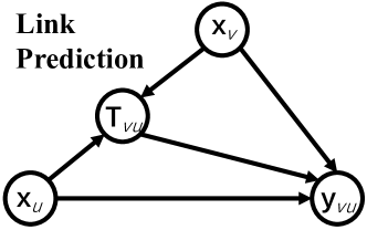
We describe the idea of link prediction with causal model which is an analogy of making medical decision with causal model. Fig. 5(a) illustrates link prediction with the causal model [19], in which the context $\textbf{x}_{v}$ and $\textbf{x}_{u}$ are representations of node $v$ and node $u$, the treatment T is defined based on the graph structure information, the outcome $y_{vu}$ is the link existence between node $v$ and node $u$. By learning from both factual outcomes Y and the counterfactual outcomes $\textbf{Y}^{CF}$ obtained from the factual treatment T and counterfactual treatment $\textbf{T}^{CF}$, the causal relationship between graph structure and link existence is captured to improve node representations.

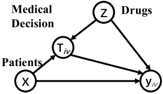
The target of the proposed medical decision problem is to explore “will patients in the same group take drugs with antagonistic effects?”. As shown in Fig. 5(b), we consider the representations of patients $\mathbf{X}$ and drugs $\mathbf{Z}$ as context and medication use $\mathbf{Y}$ as outcome, where $\mathbf{X}$ denotes the matrix formed by the combination of all patient features $\{\mathbf{x}_{1},\mathbf{x}_{2},\cdots\}^{\top}$, $\mathbf{Z}$ denotes the matrix formed by the combination of all drug features $\{\mathbf{z}_{1},\mathbf{z}_{2},\cdots\}^{\top}$ and $\mathbf{Y}$ denotes the matrix formed by the combination of patients’ medication use $\{\mathbf{y}_{1},\mathbf{y}_{2},\cdots\}^{\top}$. Since the treatment between patient $S_{i}$ and drug $D_{v}$ may be influenced by the medical decision of other similar patients as well as the DDI with other drugs, we define treatment $\mathbf{T}_{iv}$ based on the representations of all the patients $\mathbf{X}$ and drugs $\mathbf{Z}$. In summary, the treatment $\mathbf{T}$ is defined in three steps. Firstly, we define the treatment matrix $\mathbf{T}$ as $\mathbf{T}_{iv}=1$ if patient $S_{i}$ and drug $D_{v}$ have a link in the observed data, and $\mathbf{T}_{iv}=0$ otherwise. Then we cluster the patients by a clustering method such as $K$-means [20] denoted as $c:\mathbf{X}\rightarrow N$ that outputs the index of cluster that each patient belongs to, where the number of clusters is determined by the number of chronic diseases in the observed data. We set the treatment $\mathbf{T}_{jv}=1$ if $c(S_{i})=c(S_{j})$ and $\mathbf{T}_{iv}=1$ in the second step. In the final step, we assume that treatment $\mathbf{T}_{iu}=1$ if $e_{vu}=1$ and $\mathbf{T}_{iv}=1$ according to the DDI graph in Section IV-A1.

Then we find the nearest neighbor with the opposite treatment for each patient-drug pair and use the nearest neighbor’s outcome as a counterfactual link. Formally, $\forall(S_{i},D_{v})\in S\times V$, its counterfactual link $(S_{j},D_{u})$ is defined as

$$(S_{j},D_{u})=\mathop{\arg\min}\limits_{S_{j}\in S,D_{u}\in V}\{\rm{dis}(\mathbf{x}_{i},\mathbf{x}_{j})+\rm{dis}(\mathbf{z}_{v},\mathbf{z}_{u})|$$ (7)

$$\mathbf{T}_{ju}=1-\mathbf{T}_{iv},\rm{dis}(\mathbf{x}_{i},\mathbf{x}_{j})<\gamma_{p},\rm{dis}(\mathbf{z}_{v},\mathbf{z}_{u})<\gamma_{d}\},$$

where $\rm{dis}(\cdot,\cdot)$ is specified as Euclidean distance, $\mathbf{x}_{i}\in\mathbb{R}^{d_{1}}$ and $\mathbf{x}_{j}\in\mathbb{R}^{d_{1}}$ denote the original feature of patient $S_{i}$ and patient $S_{j}$, $\mathbf{z}_{v}\in\mathbb{R}^{d_{2}}$ and $\mathbf{z}_{u}\in\mathbb{R}^{d_{2}}$ denote the original feature of drug $D_{v}$ and drug $D_{u}$, $\gamma_{p}$ and $\gamma_{d}$ are hyperparameters that define the maximum distance that two patients and two drugs are considered as similar, respectively. Finally, we define the counterfactual treatment matrix $\mathbf{T}^{CF}$ and counterfactual adjacency matrix $\mathbf{Y}^{CF}$ as

$$\mathbf{T}^{CF}_{iv},y^{CF}_{iv}=\left\{\begin{array}[]{ll}1-\mathbf{T}_{iv},y_{ju}&,\ \rm{if\ }\exists(S_{j},D_{u})\in S\times V\\ &\rm{satisfies\ Eq.\ }\eqref{cflink};\\ \mathbf{T}_{iv},y_{iv}&,\ \rm{otherwise}.\\ \end{array}\right.$$ (8)

Different from traditional link prediction that only takes the observed outcomes $\mathbf{Y}$ as the training target, we take counterfactual outcomes $\mathbf{Y}^{CF}$ as the augmented training data for MDGCN training.

(a) Link prediction with causal model. The treatment $\mathbf{T}_{vu}$ is only related to the representations of node $v$ and node $u$.

(b) Medical decision with causal model. The treatment $\mathbf{T}_{iv}$ is related to the representations of all the patients $\mathbf{X}$ and drugs $\mathbf{Z}$.

Figure 5: Causal model improves patient and drug representation learning.

IV-B2 MDGCN

We divide MDGCN into an encoder and a decoder. The encoder is used to update patient and drug representations, and the decoder is used to predict patients’ medication use.

MDGCN Encoder: In the initial step, each patient and drug is associated with an original feature. Then two fully connected layers (FC) are leveraged to map the feature representations of all patients and drugs respectively to the same feature dimension as follows:

$$\mathbf{h}_{i}=\sigma(\mathbf{W}_{1}\mathbf{x}_{i}+\mathbf{b}_{1}),i=1,2,\cdots,m,$$ (9)

$$\mathbf{h}_{v}=\sigma(\mathbf{W}_{2}\mathbf{z}_{v}+\mathbf{b}_{2}),v=1,2,\cdots,|V|,$$ (10)

where $h_{i}$ and $h_{v}$ denote the hidden representations of patient $S_{i}$ and drug $D_{v}$, respectively; $\sigma(\cdot)$ denotes an element-wise activation function, $W_{1}\in\mathbb{R}^{d_{3}\times d_{1}}$, $W_{2}\in\mathbb{R}^{d_{3}\times d_{2}}$ and $b_{1}\in\mathbb{R}^{d_{3}}$, $b_{2}\in\mathbb{R}^{d_{3}}$ are learnable parameters of the fully connected layers.

After mapping the original features of patients and drugs to the same dimension, we use MDGCN to update the hidden representations of drugs. In MDGCN, the feature transformation and nonlinear activation functions are abandoned, it only adopts the simple weighted sum aggregator to update the node features. The graph convolutional operation is defined as:

$$\mathbf{h}_{i}^{(t)}=\sum_{v\in\mathcal{N}_{i}}\frac{1}{\sqrt{|\mathcal{N}_{i}|}\sqrt{|\mathcal{N}_{v}|}}\mathbf{h}_{v}^{(t-1)},$$ (11)

$$\mathbf{h}_{v}^{(t)}=\sum_{i\in\mathcal{N}_{v}}\frac{1}{\sqrt{|\mathcal{N}_{v}|}\sqrt{|\mathcal{N}_{i}|}}\mathbf{h}_{i}^{(t-1)},$$ (12)

where $\mathbf{h}_{i}^{(t)}$ and $\mathbf{h}_{v}^{(t)}$ respectively denote the updated hidden representation of patient $S_{i}$ and drug $D_{v}$ after $t$ layers propagation, $\mathbf{h}_{i}^{(0)}$ is equal to $\mathbf{h}_{i}$ calculated by Eq. (9) and $\mathbf{h}_{v}^{(0)}$ is equal to $\mathbf{h}_{v}$ calculated by Eq. (10), $\mathcal{N}_{i}$ denotes the set of drugs that are taken by patient $S_{i}$, $\mathcal{N}_{v}$ denotes the set of patients that are taking drug $D_{v}$.

After $T^{\prime}$ layers of graph convolutional operation, the hidden representations obtained at each layer are combined to form the final representation of drug $D_{v}$:

$$\mathbf{h}^{\prime}_{v}=\sum_{t=0}^{T^{\prime}}\beta_{t}\mathbf{h}_{v}^{(t)},\vspace{-0.1cm}$$ (13)

where $\beta_{t}\geq 0$ is a hyperparameter to represent the importance of the $t$-th layer representation in constituting the final representation. Note that the target node’s feature will be added at $t=0$, so we don’t need to add the target node’s feature in Eq. (11) and (12). Since representations at different layers capture different semantics, e.g., the first layer smooths patients and drugs that have interactions, the second layer smooths drugs that have overlap with interacted patients, and higher-layers capture higher-order proximity [21]. Hence, this layer combination operation will make the drugs’ representations more similar to those of patients with their corresponding diseases.

MDGCN Decoder: As shown in Fig. 3, there are many drugs to treat the same type of disease, for example, Doxazosin, Terazosin and Prazosin can all be used to treat hypertension, so how to personalize and suggest more appropriate drugs according to the features of the patient is the challenge to be solved in this paper. To obtain personalized medication suggestions, we adopt the hidden representation $\mathbf{h}_{i}$ obtained from Eq. (9) of the patient $S_{i}$ to predict his/her medication use. Compared with the patient representations obtained after MDGCN, the patient representations before MDGCN are more differentiated because there is no over-smoothing of patient representations resulting from aggregation of similar drug representations. In Section V-B, we compare the personalization of patient representations before and after MDGCN experimentally.

Next, we add DDI relation representations shared in Eq. (1) to the final drug representation $\mathbf{h}^{\prime}_{v}$, i.e., $\mathbf{h}^{\prime}_{v}=\mathbf{h}^{\prime}_{v}+\mathbf{z}_{v}$. Based on MLP, the encoder of MDGCN is defined as:

$$\hat{y}_{iv}=f^{(t)}_{\mathbf{\Theta_{2}}}([\mathbf{h}_{i}^{\top}\odot\mathbf{h}^{\prime}_{v},\mathbf{T}_{iv}]),$$ (14)

$$\hat{y}^{CF}_{iv}=f^{(t)}_{\mathbf{\Theta_{2}}}([\mathbf{h}_{i}^{\top}\odot\mathbf{h}^{\prime}_{v},\mathbf{T}^{CF}_{iv}]),$$ (15)

where $f^{(t)}_{\mathbf{\Theta_{2}}}$ denotes the MLP with parameters $\mathbf{\Theta}_{2}$, $[\cdot,\cdot]$ represents the concatenation of vectors, $\odot$ represents Hadamard Product.

System Output: At last, we combine the medical suggestion and the corresponding medical explanations obtained through the MS module, thus constructing the system output to be displayed to the doctors.

Figure 6: Given the corresponding factual and counterfactual treatments, MDGCN is trained to predict factual and counterfactual links. The different colored patients indicate that they belong to different clusters. The red (blue) lines between drugs indicate antagonistic (synergistic) effects. The black (yellow) lines between patients and drugs indicate factual (counterfactual) links.

IV-B3 Model Training

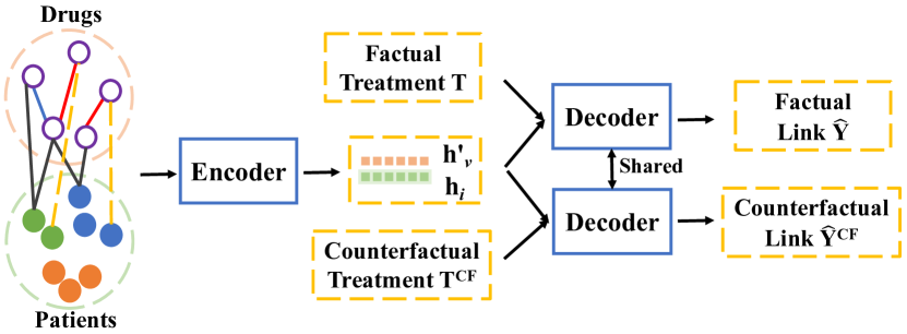
The training process of MDGCN is shown in Fig. 6. During the model training, we predict factual links and counterfactual links and optimize towards $\mathbf{Y}$ and $\mathbf{Y}^{CF}$, respectively. We adopt 1:1 negative sampling to sample negative edges for training, and then train the model by the cross-entropy loss functions defined as:

$$\mathcal{L}_{C}=-\sum_{i}^{m}\sum_{v\in\mathcal{N}_{i}}[y_{iv}\mathrm{log}(\hat{y}_{iv})+(1-y_{iv})\mathrm{log}(1-\hat{y}_{iv})],$$ (16)

$$\mathcal{L}_{CF}=-\sum_{i}^{m}\sum_{v\in\mathcal{N}_{i}}[y^{CF}_{iv}\mathrm{log}(\hat{y}^{CF}_{iv})+(1-y^{CF}_{iv})\mathrm{log}(1-\hat{y}^{CF}_{iv})].\vspace{-0.2cm}$$ (17)

The overall training loss of our model is:

$$\mathcal{L}=\mathcal{L}_{C}+\delta\mathcal{L}_{CF},\vspace{-0.1cm}$$ (18)

where $\delta$ is a hyperparameter to control the weight of counterfactual outcome estimation loss.

IV-C Medical Support Module

Given a set of suggested drugs to a patient by the decision support system, we may want to know further why the system suggests these drugs to him/her, or to what extent this suggestion makes sense. To this end, in the Medical Support (MS) module, we utilize a subgraph querying algorithm to find the closest dense subgraph containing the suggested drugs in DDI. With this subgraph, we define a Suggestion Satisfaction measurement, analyze the synergistic and antagonistic interactions between the suggested drugs and explain our suggestions. In this module, we first introduce the definition of the closest dense subgraph, then illustrate the algorithm to find the closest dense subgraph in DDI. At last, we define the Suggestion Satisfaction measurement to explain the suggestions.

IV-C1 Problem Definitions

While there are many choices of closeness on graphs, in this work, we use the closest truss community definition [22] based on triangles to find the closest dense subgraph first.

Definition 5 ($p$-truss)

A triangle in $G$ is a cycle of length 3. Let $D_{u},D_{v},D_{w}\in V$ be the three vertices on the cycle, and we denote this triangle by $\triangle_{uvw}$. Then the support of an edge $e_{uv}$ $\in E$ in $G$, denoted by $sup(e_{uv},G)$, is defined as the number of triangles in $G$ containing $e_{uv}$, i.e., $|\{\triangle_{uvw}:D_{w}\in V\}|$. A subgraph is $p$-truss if the support number of all the edges is no less than $(p-2)$. The truss number of an edge is defined as the maximum value of $p$ that this edge can contain in the $p$-truss subgraph.

Then the closest truss community is formally defined as:

Definition 6 (Closest Truss Community (CTC))

Given a graph $G$ and a set of query nodes $Q$, $G^{\prime}$ is a closest truss community (CTC), if $G^{\prime}$ satisfies the following two conditions: (1) Connected $p$-Truss: $G^{\prime}$ is a connected $p$-truss containing $Q$ with the largest $p$, i.e., $Q\subseteq G^{\prime}\subseteq G$ and $\forall e\in E(G^{\prime}),sup(e,G^{\prime})\leq(p-2)$; (2) Smallest Diameter: $G^{\prime}$ is a subgraph of smallest diameter satisfying condition (1). That is, $\nexists G^{\prime\prime}\subseteq G^{\prime}$, such that $diam(G^{\prime\prime})\leq diam(G^{\prime})$, and $G^{\prime\prime}$ satisfies condition (1), where $diam(G^{\prime})$ denotes the diameter of $G^{\prime}$.

In our task, given a set of suggested drugs $Q=\{{D_{q}}_{1},{D_{q}}_{2},\dots,{D_{q}}_{k}\}$, we find the closest truss community in the DDI graph which contains all the suggested drugs, and these drugs in the subgraph connect densely through either synergistic or antagonistic interactions. In such a discovered subgraph, we can analyze the drug interactions and explain why we suggest these drugs.

IV-C2 Subgraph Querying

To find out this closest dense subgraph, we use the community search algorithms in [22]. In particular, it first computes a Steiner tree and then extends the Steiner tree into a dense subgraph. In this subgraph, we find a closest dense subgraph. The main algorithms used in this process include Steiner Tree Computation and Truss Decomposition. We briefly describe them below.

Steiner Tree Computation

Given a graph $G$ and query nodes $Q$, it firstly constructs a complete distance graph $G^{\prime}$ of query nodes where the distance is the truss distance defined in [22]. It then finds a minimum spanning tree $T_{s}$ of $G^{\prime}$ , and then constructs another graph $H$ by replacing each edge of tree $T_{s}$ by its corresponding shortest path in $G^{\prime}$, and finally finds a minimum spanning tree of $H$ and deletes leaf edges. The detailed algorithm can be found in [23].

Truss Decomposition

To compute the truss number of each edge, we use the truss decomposition algorithm [24]. It first computes the support number for each edge and sorts all the edges in ascending order of their support. Then it deletes the edges with the smallest support and updates other edges’ support. The truss number of one edge is the updated support number when it is deleted. After all the edges are deleted, the truss number of each edge is computed.

The entire algorithm is listed in Algorithm 1. We first do truss decomposition [24] on the DDI graph $G$ (line 1), then use the truss distance function [22] to compute the Steiner Tree $T_{s}$ [23] (line 2). Based on $T_{s}$, we extend it to a dense subgraph $G_{0}^{\prime}$ that the truss number of each edge is no less than the minimum truss number of $T_{s}$ (line 3-7). On this dense subgraph $G_{0}^{\prime}$, we do truss decomposition (line 8) and find the connected $p$-truss community with maximum $p$ it can find (line 9). Then we iteratively shrink the subgraph by deleting the furthest nodes while maintaining the truss property (line 10-14). The final closest related subgraph is the subgraph with the smallest diameter during the iterations (line 15).

Algorithm 1 Subgraph Querying

Input: DDI graph: $G=(V,E)$,

suggested drugs: $Q=\{{D_{q}}_{1},{D_{q}}_{2},\dots,{D_{q}}_{k}\}$

Output: related subgraph of suggested drugs: $G_{sub}=\{{D_{1}},{D_{2}},\dots\}$.

1:  Do truss decomposition on $G$

2:  Compute the Steiner Tree $T_{s}$ containing suggested drugs

3:  $G_{0}^{\prime}\leftarrow T_{s}$

4:  $p^{\prime}\leftarrow\min_{e^{\prime}\in T_{s}}truss(e^{\prime})$:

5:  while size of $G_{0}^{\prime}<n_{0}$

6:       if ($e$ is an adjacent edge to $G_{0}^{\prime}$ and $truss(e)\geq p^{\prime}$)

7:            $G_{0}^{\prime}\leftarrow G_{0}^{\prime}\cup e$

8:  Do truss decomposition on $G_{0}^{\prime}$

9:  Find maximum connected $p$-truss subgraph containing $Q$ in $G_{0}^{\prime}$

10:  $i\leftarrow 0$

11:  while (connected($Q$))

12:       $G^{\prime}_{i+1}\leftarrow$ delete the furthest nodes of $G^{\prime}_{i}$

13:       Maintain $p$-truss property of $G^{\prime}_{i+1}$

14:       $i\leftarrow i+1$

15:  return $G_{sub}\leftarrow\arg\min_{G^{\prime}\in\{G^{\prime}_{0},G^{\prime}_{1},...\}}dist(G^{\prime},Q)$

IV-C3 Measurement

For a suggestion with $k$ drugs, we use Suggestion Satisfaction (SS) to measure its rationality.

Definition 7 (Suggestion Satisfaction (SS))

Let the closest dense subgraph of the DDI graph w.r.t. the suggested drugs be $G_{sub}$ with $n^{\prime}$ nodes. $r^{in}_{pos}$ and $r^{in}_{neg}$ denote the number of synergistic edges and antagonistic edges between the $k$ suggested drugs respectively. $r^{out}_{neg}$ is the number of antagonistic edges between the $k$ suggested drugs and $n^{\prime}-k$ non-suggested drugs. SS is defined as follows:

$$SS=\alpha\frac{2(r^{in}_{pos}+1)}{(r^{in}_{neg}+1)(k(k-1)+2)}+(1-\alpha)\frac{r^{out}_{neg}}{k(n^{\prime}-k)},$$ (19)

where the first term explains the synergistic effect between the suggested drugs, while the second explains the antagonistic effect between the suggested drugs and the non-suggested drugs. $\alpha\in(0,1)$ is a hyperparameter that balances the two terms. We expect better synergy between the suggested drugs and greater antagonism with the non-suggested drugs, so a larger SS can denote a more appropriate drug suggestion.

The MS module explains the medication suggestions from a visual perspective (subgraphs) and a numerical perspective (SS), giving the doctors a more reliable, easier to understand and more visual explanation of the suggestion.

V Experiments

In our experiments, we first evaluate the performance of DSSDDI for personalized drug suggestions and compare it with baseline methods. Then we conduct ablation study to prove the superiority of DDIGCN. Next, we demonstrate the explainablility of DSSDDI with the measurement of SS. Finally, we validate the model’s effectiveness on a public diagnostic data set MIMIC-III [9].

V-A Experimental Setup

V-A1 Baselines

We compare DSSDDI with the following baselines.

Traditional Methods:

• UserSim: Given the problem formulation of our decision support system, we evaluate the effectiveness of the system by predicting the medication use of the unobserved patients, who are not involved in the model training process. Hence, we design a naive baseline method, called User Similarity (UserSim). The suggestion scores of each drug for unobserved patients are obtained by weighting the medication use of each observed patient using the similarity between each observed patient and unobserved patients as weights, and calculated by the following equation:

  $$\mathbf{Y}_{\mathcal{U}}=\text{cosine\_similarity}(\mathbf{X}_{\mathcal{U}},\mathbf{X}_{\mathcal{O}})\cdot\mathbf{Y}_{\mathcal{O}},\vspace{-0.2cm}$$ (20)

  where $\mathbf{Y}_{\mathcal{U}}$ denotes the prediction score matrix for unobserved patients, $\mathbf{X}_{\mathcal{O}}$ and $\mathbf{X}_{\mathcal{U}}$ denote the feature matrix of observed patients and unobserved patients, and $\mathbf{Y}_{\mathcal{O}}$ denotes the medication use of observed patients.

• ECC [25]: Ensemble Classifier Chain (ECC) is a popular multi-label classification method that models the correlation between labels by feeding both input and prediction by the previous classifier into the next classifier. We employ Logistic Regression (LR) [26] as binary classifiers for each label.

• SVM [27]: Bao et al. [28] demonstrate the good performance of support vector machine (SVM) as a traditional machine learning method for medication suggestion.

Graph Learning-based Methods:

• GCMC [29]: A recommendation system organizes historical user behaviors as a holistic interaction graph and employs a GCN encoder to generate representations. GCMC focuses on explicit feedback, constructs multiple adjacency matrices according to the type of score, and uses different weight matrices to decode different types of edges.

• LightGCN [21]: This method simplifies the embedding propagation process by eliminating the nonlinear activation function and feature transformation matrix to obtain a light GCN model.

• SafeDrug [6]: A model equipped with a global Message Passing Neural Network (MPNN) module to capture drugs’ molecule structures and a local bipartite learning module to explicitly model drug-drug interactions. It employs Gated Recurrent Unit (GRU) [30] to encode patients’ features from patients’ past visits.

• Bipar-GCN [4]: This method is specifically designed for bipartite graph. The patient embeddings and drug embeddings are obtained by training two structurally identical neural networks called patient-oriented NN and drug-oriented NN with different parameters, respectively.

• CauseRec [5]: A causal recommendation model that learns patient representations by generating counterfactual patient behavior sequences from patients’ past visits.

Variants of DSSDDI:

• DSSDDI(GIN): DSSDDI with a common GCN model GIN [13] as backbone.

• DSSDDI(SGCN): DSSDDI with a signed GCN model SGCN [14] as backbone.

• DSSDDI(SiGAT): DSSDDI with an attention-based signed GCN model SiGAT [15] as backbone.

• DSSDDI(SNEA): DSSDDI with an attention-based signed GCN model SNEA [16] as backbone.

V-A2 Metrics

We split all patients into training set, validation set and test set in the ratio of 5:3:2, the hyperparameter selection is based on the prediction performance on the validation set. We adopt SS@$k$ (top-$k$ Suggestion Satisfaction) defined in Eq. (19) to assess the explainability of drug suggestions for each method. We also use Precision@$k$, Recall@$k$ and NDCG@$k$ (Normalized Discounted Cumulative Gain) [31] to measure the effectiveness of all methods:

(1) Precision@$k$ and Recall@$k$ are defined as:

$$Precision@k=\frac{\sum_{j}|P(j)\cap Q(j)|}{\sum_{j}|P(j)|},$$ (21)

$$Recall@k=\frac{\sum_{j}|P(j)\cap Q(j)|}{\sum_{j}|Q(j)|},$$ (22)

where $P(j)$ represents the set of the $k$ drugs suggested to the patient $S_{j}$, $Q(j)$ represents the set of drugs that the patient $S_{j}$ is taking.

(2) NDCG@$k$ is defined as:

$$NDCG@k=\frac{1}{|\mathcal{U}|}\sum_{j\in\mathcal{U}}\frac{DCG_{j}@k}{IDCG_{j}},$$ (23)

where $DCG_{j}@k$ is the Discounted Cumulative Gain of the $k$ drugs suggested to the patient $S_{j}$, and $IDCG_{j}$ is the ideal DCG for the patient $S_{j}$. $DCG_{j}@k$ is defined as:

$$DCG_{j}@k=\sum_{s=1}^{k}\frac{2^{rel_{s}}-1}{\mathrm{log}_{2}(s+1)},\vspace{-0.1cm}$$ (24)

where $rel_{s}$ is the graded relevance of the result at position $s$. NDCG@$k$ takes a value between 0 and 1, and the larger the value the greater the suggestion scores for those drugs the patient is taking.

TABLE I: Medication suggestion performance comparison between the proposed method and baseline methods on Chronic data set (the best results are in bold and the second results are underlined).

Method	Precision@6	Recall@6	NDCG@6	Precision@5	Recall@5	NDCG@5	Precision@4	Recall@4	NDCG@4
UserSim	0.0982	0.2227	0.1432	0.0971	0.2209	0.1426	0.0977	0.2181	0.1418
ECC	0.0214	0.0537	0.0328	0.0252	0.0519	0.0321	0.0060	0.0108	0.0127
SVM	0.0670	0.2166	0.2062	0.0635	0.1681	0.1847	0.0787	0.1653	0.1838
GCMC	0.1362	0.5310	0.3652	0.1447	0.4541	0.3181	0.1638	0.4057	0.3146
LightGCN	0.2073	0.7348	0.6012	0.2358	0.7245	0.5681	0.2581	0.6509	0.5436
SafeDrug	0.0863	0.3098	0.2267	0.1000	0.2952	0.2227	0.1250	0.2952	0.2233
Bipar-GCN	0.1741	0.6267	0.4817	0.1952	0.5911	0.4667	0.2172	0.5363	0.4418
CauseRec	0.1707	0.1025	0.5117	0.1124	0.4492	0.3030	0.3186	0.2468	0.1799
DSSDDI(SiGAT)	0.2214	0.8215	0.6482	0.2514	0.7834	0.6323	0.2876	0.7266	0.6076
DSSDDI(SNEA)	0.2192	0.7854	0.5949	0.2447	0.7364	0.5744	0.2740	0.6684	0.5442
DSSDDI(GIN)	0.2272	0.8407	0.6836	0.2534	0.8104	0.6873	0.2900	0.7704	0.6575
DSSDDI(SGCN)	0.2348	0.8521	0.6850	0.2670	0.8153	0.6717	0.3077	0.7746	0.6680
Method	Precision@3	Recall@3	NDCG@3	Precision@2	Recall@2	NDCG@2	Precision@1	Recall@1	NDCG@1
UserSim	0.0970	0.1970	0.1324	0.1370	0.1348	0.1033	0.0889	0.0088	0.0108
ECC	0.0072	0.0098	0.0123	0.0108	0.0098	0.0135	0.0192	0.0094	0.0204
SVM	0.1050	0.1649	0.1863	0.1575	0.1639	0.1970	0.3029	0.1552	0.2536
GCMC	0.1791	0.3437	0.2898	0.1971	0.2392	0.2406	0.1815	0.1428	0.2344
LightGCN	0.2925	0.5854	0.5436	0.3347	0.4021	0.4187	0.4231	0.2605	0.3786
SafeDrug	0.1206	0.2182	0.1872	0.1280	0.1536	0.1609	0.1406	0.0902	0.1406
Bipar-GCN	0.2484	0.4671	0.4118	0.2861	0.3672	0.3734	0.3377	0.2197	0.3377
CauseRec	0.2122	0.1595	0.1064	0.1665	0.1250	0.2494	0.1484	0.1484	0.1484
DSSDDI(SiGAT)	0.3361	0.6519	0.5745	0.3912	0.5261	0.5214	0.4531	0.3206	0.4531
DSSDDI(SNEA)	0.3133	0.5795	0.5059	0.3365	0.4242	0.4375	0.4038	0.2667	0.4038
DSSDDI(GIN)	0.3554	0.6918	0.6256	0.4261	0.5926	0.5842	0.4916	0.3989	0.5565
DSSDDI(SGCN)	0.3670	0.7027	0.6378	0.4297	0.5903	0.5933	0.5300	0.3743	0.5300

V-A3 Implementation Details

We use Adam [32] optimizer to minimize the overall loss $\mathcal{L}$ of MDGCN and MSE loss $\mathcal{L}_{M}$ of DDIGCN. The learning rates used to optimize MDGCN and DDIGCN are 0.01 and 0.001, respectively. The training epochs for MDGCN and DDIGCN are set to 1000 and 400. The hidden representation size is fixed to 64. For MDGCN, LeakyReLU [33] activation is used after the fully connected layers. The size of the graph convolution layer we set for MDGCN is 2. We set the hyperparameters $\beta_{t}=1/(t+2)$ and $\delta=1$. For DDIGCN, we set the layer sizes as 3 for the graph convolution. Batch normalization [34] and ReLU [33] activation are applied after each layer.

V-B Experimental Results of Medication Suggestion

The experimental results for medication suggestions are shown in Table I. We observe that DSSDDI achieves the best results for almost all $k$ values in $1,\ldots,6$. When compared with the graph learning-based methods, we find that traditional methods perform much worse. This is because traditional methods cannot capture latent patient features, making them difficult to provide effective suggestions based only on the patients’ numerical features.

(a) Cosine similarity between patient representations.

(b) Cosine similarity between drug representations.

Figure 7: Comparison of cosine similarity between patient (drug) representations obtained from DSSDDI and LightGCN. Closer to red means that the representations are more similar and closer to blue means that they are less similar. (a) We sample 100 patients in the test set of patients. (b) 86 drugs are included in the comparison of their similarity to each other.

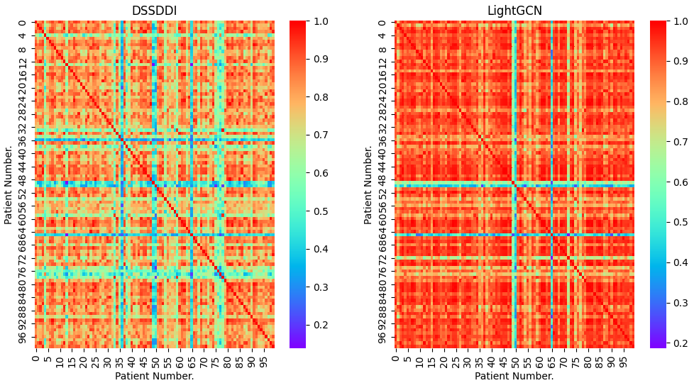
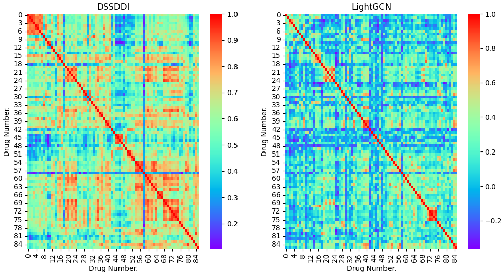
In addition, we observe that DSSDDI performs better than the graph learning-based methods. The reason is that the graph convolution process smooths the patient representations. Specifically, DSSDDI employs the patient representations before the graph convolution layer to predict the patient’s medication use, which ensures that the patient representations during model training will not be affected by similar drug representations. However, in graph learning-based methods, patient representations are updated through graph convolution, resulting in similar representations of most patients. To validate this speculation, we sample 100 patients in the test set and calculate the cosine similarity between patient representations by DSSDDI and LightGCN and plot the heat map in Fig. 7(a). As we can see, the similarity between the patient representations obtained by LightGCN is extremely high. Such similar representations make it difficult for LightGCN to identify feature differences between patients. In contrast, the patient representations obtained by DSSDDI are more distinguishable, which indicates that MDGCN avoids the over-smoothing of patient representations. Due to the high similarity between patient representations, some drugs with high similarity to patient representations will be suggested frequently, making it difficult for LightGCN to personalize the suggestions.

In addition, we calculate the cosine similarity between drug representations by DSSDDI and LightGCN and plot the heat map in Fig. 7(b). The drug representations obtained by DSSDDI are more reasonable because many drugs are related as they treat the same type of disease such as cardiovascular disease, arthritis and diabetes as shown in Fig 3. In contrast, all drug representations learned by LightGCN have low similarity.

When comparing DSSDDI with different backbones, DSSDDI(SGCN) performs best, showing that SGCN can learn better drug embeddings from synergistic and antagonistic interactions. DSSDDI(GIN) performs slightly worse than DSSDDI(SGCN). The attention-based models DSSDDI(SiGAT) and DSSDDI(SNEA) are less effective.

TABLE II: Ablation studies with different drug embeddings on Chronic data set (the best results are in bold). Here, we use SGCN, the best performing backbone model in Table I, as the backbone in DDIGCN.

Method	Precision@6	Recall@6	NDCG@6	Precision@5	Recall@5	NDCG@5	Precision@4	Recall@4	NDCG@4
w/o DDI	0.2185	0.7974	0.6427	0.2490	0.7694	0.6301	0.2891	0.7256	0.6089
One-hot	0.2095	0.7952	0.6063	0.2365	0.7537	0.5891	0.2638	0.6830	0.5574
KG	0.2135	0.8170	0.6489	0.2411	0.7761	0.6319	0.2758	0.7187	0.6067
DDIGCN	0.2348	0.8521	0.6850	0.2670	0.8153	0.6717	0.3077	0.7746	0.6680
Method	Precision@3	Recall@3	NDCG@3	Precision@2	Recall@2	NDCG@2	Precision@1	Recall@1	NDCG@1
w/o DDI	0.3413	0.6499	0.5788	0.4032	0.5277	0.5292	0.4796	0.3204	0.4796
One-hot	0.2984	0.5904	0.5150	0.3462	0.4715	0.4635	0.4147	0.2855	0.4147
KG	0.3297	0.6609	0.5810	0.3918	0.5425	0.5304	0.4591	0.3338	0.4591
DDIGCN	0.3670	0.7027	0.6378	0.4297	0.5903	0.5933	0.5300	0.3743	0.5300

V-C Superiority of DDIGCN

We conduct an ablation study to demonstrate the superiority of DDIGCN. We create the following variants by replacing the drug embedding learned by DDIGCN with three alternatives:

• Without DDI: Without adding DDI relation embeddings to the final drug embeddings $\textbf{h}^{\prime}_{v}$.

• One-hot: One-hot embeddings.

• KG: Pre-trained embeddings obtained from DRKG [10].

The results are reported in Table II. DDIGCN performs the best, which indicates that DDIGCN learns drug embeddings from the DDI relationship that is more useful for medication suggestions. DDIGCN outperforms the system without DDI module, due to its consideration of drug-drug interactions, thus avoiding numerous inappropriate suggestions. As DRKG contains many different types of entities such as genes and proteins, KG per-trained embeddings may contain much too complex information, such as the relationship between drug and genes which affect the drug suggestion performance.

TABLE III: Suggestion satisfaction comparison between the proposed method and baseline methods on $k$ medication suggestions.

k	2	3	4	5	6
UserSim	0.4987	0.2506	0.0743	0.0470	0.0220
ECC	0.5000	0.2500	0.0952	0.0455	0.0339
SVM	0.5044	0.2695	0.1050	0.0469	0.0278
GCMC	0.4979	0.2533	0.1443	0.0491	0.0634
LightGCN	0.5046	0.2544	0.1631	0.0882	0.0575
SafeDrug	0.4412	0.1812	0.0741	0.0477	0.0329
Bipar-GCN	0.5139	0.2788	0.1735	0.1183	0.0866
CauseRec	0.4957	0.2462	0.0996	0.0482	0.0299
DSSDDI(SiGAT)	0.5683	0.3237	0.2043	0.1400	0.1042
DSSDDI(SNEA)	0.5522	0.2916	0.1811	0.1253	0.0899
DSSDDI(GIN)	0.5392	0.2767	0.1743	0.1227	0.0997
DSSDDI(SGCN)	0.5427	0.3267	0.2158	0.1478	0.1083

V-D Explainability of DSSDDI

Table III compares the proposed method with baseline methods in terms of Suggestion Satisfaction (SS) with medication suggestions. DSSDDI has a significant improvement compared to other methods. In particular, compared with the best-performing baseline, DSSDDI improves $SS@6$ by 25%, $SS@5$ by 24% and $SS@4$ by 24%. Because SS takes into account not only the synergy between the $k$ suggested drugs but also the antagonism between the suggested and non-suggested drugs, we can conclude that DSSDDI is able to suggest drugs with more synergistic effects, while being able to avoid drugs with antagonistic effects from being included. By extracting these relevant drug-drug interactions as subgraphs in the DDI graph, it provides an effective explanation for the drugs suggested by the Medical Decision module.

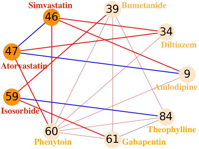
We then show a case of medication suggestion for a patient with cardiovascular disease in Fig. 8 to highlight the more reliable medication suggestions of DSSDDI compared to baseline methods from an explainable perspective. All these subgraphs were obtained according to the subgraph querying algorithm proposed in the MS module. As shown in Fig. 8(a), DSSDDI suggests Simvastatin (Drug ID (DID) 46), Atorvastatin (DID 47) and Isosorbide (DID 59). There is a synergistic effect between Simvastatin (DID 46) and Atorvastatin (DID 47) as indicated by the blue line between them. Using these two drugs is indeed beneficial in lowering lipids and improving cardiovascular disease. The suggestion by DSSDDI can also avoid antagonistic effects. For example, it does not suggest Gabapentin (DID 61) because there is an antagonistic effect between Gabapentin (DID 61) and Isosorbide (DID 59) as indicated by the red line between them. This shows that DSSDDI considers synergistic effects between the suggested drugs and avoids antagonism benefiting from the combination.

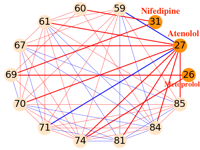
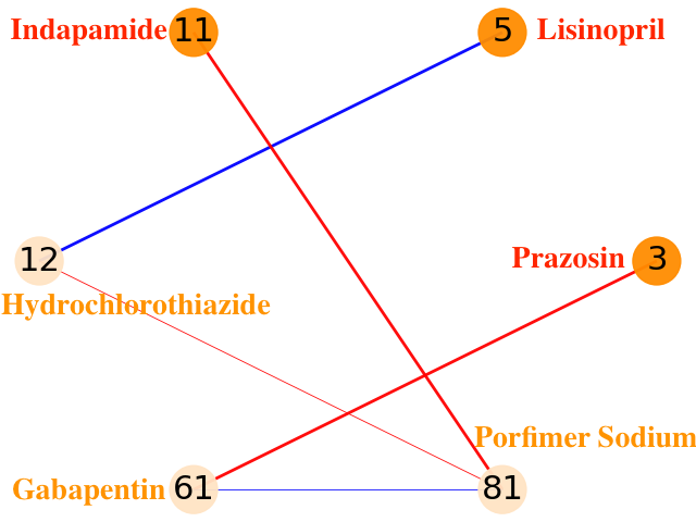
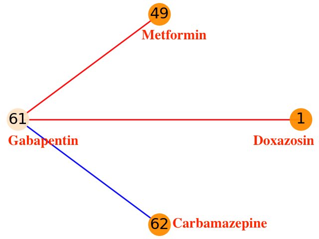
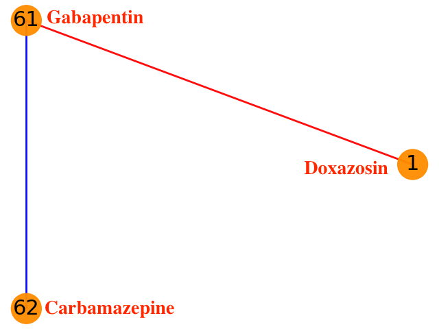
In contrast, the three drugs suggested by LightGCN, GCMC and SVM, respectively (in Figs. 8(b)-8(d)) do not have any interactions. The drugs suggested by ECC even have antagonistic interactions, i.e., Gabapentin (DID 61), a drug for epilepsy, is antagonistic to Doxazosin (DID 1) as shown in Fig. 8(e).

From this experiment, we can see that DSSDDI outputs such explainable DDI subgraphs through the Medical Support module, which can provide more convincing support for DSSDDI’s medical suggestions and make doctors’ decisions more efficient.

(a) DSSDDI

(b) LightGCN

(c) GCMC

(d) SVM

(e) ECC

Figure 8: A case of medication suggestion for a patient with cardiovascular disease. We use dark orange nodes to denote suggested drugs and light orange nodes to denote non-suggested nodes in the subgraph output by the MS module, red lines to indicate the antagonism between drugs, and blue lines to indicate the synergy between drugs. We make the edges between the non-suggested drugs transparent to highlight the interactions associated with the suggested drugs.

Figure 9: Four case studies that demonstrate the superiority of DDI. The red numbers in the Label column indicate the drugs the patient took, the blue (red) line indicates the drug-drug synergistic (antagonistic) effect, the blue (red) arrow indicates an upward or downward movement brought by the synergistic (antagonistic) effect.

TABLE IV: Medication suggestion performance comparison between the proposed method and baseline methods on MIMIC-III data set
(the best results are in bold).

Method	Precision@8	Recall@8	NDCG@8	Precision@6	Recall@6	NDCG@6	Precision@4	Recall@4	NDCG@4
UserSim	0.5396	0.2349	0.6203	0.5699	0.1869	0.6534	0.7006	0.1551	0.7557
ECC	0.6957	0.3014	0.7360	0.7786	0.2562	0.7904	0.8116	0.1795	0.8111
SVM	0.7645	0.3343	0.7829	0.8234	0.2703	0.8182	0.8313	0.1833	0.8210
GCMC	0.7924	0.3283	0.8156	0.8186	0.2656	0.8208	0.8360	0.1764	0.8392
LightGCN	0.8099	0.3548	0.8252	0.8310	0.2738	0.8378	0.8449	0.1872	0.8495
SafeDrug	0.8038	0.3549	0.8215	0.8172	0.2701	0.8308	0.8434	0.1869	0.8494
Bipar-GCN	0.7939	0.3510	0.8135	0.8172	0.2718	0.8281	0.8327	0.1856	0.8390
CauseRec	0.1218	0.1428	0.1346	0.1196	0.1130	0.1238	0.1157	0.0818	0.1162
DSSDDI(GIN)	0.8134	0.3611	0.8266	0.8352	0.2808	0.8408	0.8530	0.1932	0.8553

V-E Validation on Public Diagnostic Data

In this experiment, we evaluate medication suggestion performance using a public, real diagnostic data set, MIMIC-III [9]. It is a database comprising de-identified health-related data associated with patients who stayed in critical care units of the Beth Israel Deaconess Medical Center between 2001 and 2012. This data set includes 6350 patients, each with at least two visits. Each visit includes three types of information: medicine, diagnosis and procedure. To fit our problem setting, we use the medicine information of the last visit as the medication suggestion label to be predicted, and the diagnosis and procedure information of previous visits as the patient features. The medication suggestion performance of the proposed method and the baselines is shown in Table IV. Since only antagonistic interactions between anonymous drugs are included in the downloaded data, we cannot use signed graph-based models as the backbone, so only GIN-based results are reported in Table IV. DSSDDI outperforms all baselines, demonstrating the significant effects that the DDI brings to medical suggestions.

VI System Application

In this section, we present four cases to further illustrate the superiority of DDI in Fig. 9.

Case 1. The patient 2417 took medications DID 10, 2, 5 (in the “Label” column). LightGCN without using DDI ranks DID 10, 2 and 5 at the first, second and fifth positions, respectively. As there is a synergistic interaction between Indapamide (DID 10) and Perindopril (DID 5), our model can rank Perindopril at the fourth position (instead of the fifth) due to this synergy. Thus our model provides a more accurate suggestion by using DDI information.

Case 2. The patient 2341 took medications DID 2 and 5. LightGCN without using DDI ranks DID 2 and 5 at the first and fifth positions, respectively. It also suggests Theophylline (DID 83) and Enalapril (DID 3) at the third and fourth position. However, there is an antagonistic interaction between them, as indicated by the red line. In contrast, our model ranks DID 2 and 5 at the first and third position, and ranks DID 3 and 83 at a lower position. This suggestion is more accurate than that by w/o DDI.

Case 3. The patient 3117 took medication DID 32. LightGCN w/o DDI ranks DID 32 at the eighth position. We find Amlodipine (DID 8) and Felodipine (DID 32) are antagonistic to four common drugs, including Phenytoin, Doxazosin, Terazosin, and Prazosin. Therefore, these two are considered as similar drugs by DSSDDI. Indeed both of them are for treating hypertension. Benefiting from the message passing of DDIGCN, these two drugs can have similar representations due to interactions with many common drugs, although they do not have direct drug-drug interactions. As a result, our model ranks these two drugs at the second and fourth positions, respectively.

Case 4. In practice, we observe that some patients are taking some drugs with antagonistic effects, probably because they were facing severe medical conditions, thus had to neglect the drug-drug interactions. For instance, the patient 6 took Isosorbide (DID 58) and Metformin (DID 48) which may cause adverse drug reactions such as cholecystitis and dizziness, so DSSDDI downgrades Metformin to the sixth position. Although this suggestion is not consistent with the ground truth, it appears more reasonable from the perspective of DDI due to the antagonistic effect between the two drugs.

VII Related work

This work is related to decision support system, graph learning-based recommendation systems, causal models with graph learning and Drug-Drug Interaction models.

VII-A Decision Support System

Decision Support System is a computer software that provides a reference for medical practitioners in their clinic decision-making [35]. Recent decision support systems can be divided into knowledge-based and data-driven methods [3].

Knowledge-based methods are mainly developed based on medical guidelines and medical knowledge, for example, rule-based methods [36], semantic or associative networks [37] and Bayesian Networks [38]. These methods are generally limited in scale, due to the lack of evidence in some domains.

With the development of Machine Learning (ML), more and more decision support systems are shifting from knowledge-based methods to data-driven methods [3]. ML models such as Ensemble Classifier Chain (ECC) [25], Support Vector Machines (SVM) [39] have been widely applied to develop decision support systems. However, they rely on the quality and quantity of data provided. When there is a bias in the data used to train the ML model, this bias is captured by the model and therefore biased predictions are made which can influence human decisions. Therefore, the aim of this paper is to propose an explainable decision support system that can provide explanations for the suggested medication, which will be more beneficial for medical practitioners to make decisions.

VII-B Graph Learning-based Recommendation Systems

Since the data in most recommendation systems is essentially a graph structure, more and more graph learning methods have been applied to learn the inter-object relations in recommendation systems [40]. Random walk based recommendation system [41] has been widely adopted to capture complex, higher-order and indirect relations among a variety of nodes on the graph [42]. Graph representation learning-based recommendation system [43] encodes each node into a latent representation and then analyzes the complex relations between them. Another class of recommendation systems are built on the knowledge graph (KG) to explore latent relations among users or items connected as a heterogeneous graph[44].

Benefiting from the strength of Graph Neural Networks (GNN), a lot of GNN based recommendation systems [45, 21] are developed. GCMC [29] leverages matrix completion to obtain the latent node representations. LightGCN [21] simplifies the graph convolution by eliminating the nonlinear activation function and feature transformation matrix. Bipar-GCN [4] learns user representations and drug representations by training user-oriented and item-oriented neural networks respectively. However, these methods have the problem of over-smoothing of patient representations because many patients take similar medications. The proposed DSSDDI solves this problem by using the patient representations before the graph convolutional operation. SafeDrug [6] combines the drug molecular graph and DDI graph to predict safe medication combinations. However, this method is difficult for new patients because it relies on medication information from patient’s past visits to generate patient features.

VII-C Causal Models with Graph Learning

As causal models capture the causal relationship between outcomes and inputs, a series of studies have focused on using causal models to enhance the inference stage of ML models [7, 8, 46]. Recently, several causal models with graph learning have gained increasing attention [47, 48, 49]. Based on causal models, counterfactual causal inference [18] aims to find out the causal relationship between treatments and outcomes by exploring whether the outcomes would be different if the treatment is different. Zhao et al. [19] employ the counterfactual causal model to improve graph representation learning. CauseRec [5] generates counterfactual patient behavior sequences to learn patient representations. However, it relies mainly on medication information from patients’ past visits, making it difficult to cope with many new patients on their first visit. In this paper, we explore the application of the counterfactual causal model to medical decision.

VII-D Drug-Drug Interaction Models

Recently, a lot of methods have been proposed for learning low-dimensional drug embeddings which are then used for downstream tasks such as Drug-Drug Interaction (DDI) prediction or drug classification [50]. These approaches can be mainly classified into relational-based approaches and network structure-based approaches.

Relational-based approaches use knowledge graph to capture multi-relational information from different edge relations [51]. For example, Zitnik et al. [52] employ a multi-relational network to identify the relation between drugs by regrading each relation as a matrix. TransE [11] and TransH [53] are also commonly used knowledge representation learning models being used to learn drug embeddings and the relations [10].

Unlike the relational-based approaches, network structure-based approaches employ Graph Neural Networks to learn the drug embeddings through aggregating the information of their neighbors [54]. For instance, Feng et al. [55] apply GCN to capture the network structure information for drugs in the DDI network. Wang et al. [56] develop a dual-attention model to extract features from the molecular and the DDI graphs.

VIII Conclusion

In this paper, we design a decision support system called DSSDDI for assisting doctors in making clinical decisions for patients with chronic diseases. Based on the external knowledge of drug-drug interactions, DSSDDI is able to obtain not only reliable medication suggestions through causal relationships in the Medical Decision module, but also the explanations for the suggestions through the Medical Support module. DSSDDI achieves superior performance to the baseline approaches for medication suggestion. In addition, it also provides explanation to the suggestions. In future work, we plan to complement the decision support system with some medical image features and to enable the search for etiological and explainable factors on the images.

References

- [1] B. C. Wimmer, A. J. Cross, N. Jokanovic, M. D. Wiese, J. George, K. Johnell, B. Diug, and J. S. Bell, “Clinical outcomes associated with medication regimen complexity in older people: a systematic review,” JAGS, vol. 65, no. 4, pp. 747–753, 2017.
- [2] S. Dumbreck, A. Flynn, M. Nairn, M. Wilson, S. Treweek, S. W. Mercer, P. Alderson, A. Thompson, K. Payne, and B. Guthrie, “Drug-disease and drug-drug interactions: systematic examination of recommendations in 12 uk national clinical guidelines,” BMJ, vol. 350, 2015.
- [3] A. Awaysheh, J. Wilcke, F. Elvinger, L. Rees, W. Fan, and K. L. Zimmerman, “Review of medical decision support and machine-learning methods,” Veterinary pathology, vol. 56, no. 4, pp. 512–525, 2019.
- [4] Y. Jin, W. Zhang, X. He, X. Wang, and X. Wang, “Syndrome-aware herb recommendation with multi-graph convolution network,” in ICDE 2020. IEEE, pp. 145–156.
- [5] S. Zhang, D. Yao, Z. Zhao, T. Chua, and F. Wu, “Causerec: Counterfactual user sequence synthesis for sequential recommendation,” in SIGIR ’21. ACM, 2021, pp. 367–377.
- [6] C. Yang, C. Xiao, F. Ma, L. Glass, and J. Sun, “Safedrug: Dual molecular graph encoders for recommending effective and safe drug combinations,” in IJCAI 2021, pp. 3735–3741.
- [7] X. Hu, K. Tang, C. Miao, X.-S. Hua, and H. Zhang, “Distilling causal effect of data in class-incremental learning,” in CVPR, 2021, pp. 3957–3966.
- [8] X. Yang, F. Feng, W. Ji, M. Wang, and T.-S. Chua, “Deconfounded video moment retrieval with causal intervention,” in SIGIR, 2021, pp. 1–10.
- [9] A. E. Johnson, T. J. Pollard, L. Shen, L.-w. H. Lehman, M. Feng, M. Ghassemi, B. Moody, P. Szolovits, L. Anthony Celi, and R. G. Mark, “Mimic-iii, a freely accessible critical care database,” Scientific data, vol. 3, no. 1, pp. 1–9, 2016.
- [10] V. N. Ioannidis, X. Song, S. Manchanda, M. Li, X. Pan, D. Zheng, X. Ning, X. Zeng, and G. Karypis, “Drkg - drug repurposing knowledge graph for covid-19,” 2020.
- [11] A. Bordes, N. Usunier, A. Garcia-Duran, J. Weston, and O. Yakhnenko, “Translating embeddings for modeling multi-relational data,” NeurIPS, vol. 26, 2013.
- [12] H. Liu, W. Zhang, B. Zou, J. Wang, Y. Deng, and L. Deng, “Drugcombdb: a comprehensive database of drug combinations toward the discovery of combinatorial therapy,” Nucleic acids research, vol. 48, no. D1, pp. D871–D881, 2020.
- [13] K. Xu, W. Hu, J. Leskovec, and S. Jegelka, “How powerful are graph neural networks?” in ICLR, 2018.
- [14] T. Derr, Y. Ma, and J. Tang, “Signed graph convolutional networks,” in ICDM 2018. IEEE Computer Society, pp. 929–934.
- [15] J. Huang, H. Shen, L. Hou, and X. Cheng, “Signed graph attention networks,” in ICANN 2019, ser. Lecture Notes in Computer Science, vol. 11731. Springer, 2019, pp. 566–577.
- [16] Y. Li, Y. Tian, J. Zhang, and Y. Chang, “Learning signed network embedding via graph attention,” in AAAI 2020. AAAI Press, 2020, pp. 4772–4779.
- [17] J. O. Berger, “Certain standard loss functions,” Statistical decision theory and Bayesian Analysis, pp. 60–64, 1985.
- [18] S. L. Morgan and C. Winship, Counterfactuals and causal inference. Cambridge University Press, 2015.
- [19] T. Zhao, G. Liu, D. Wang, W. Yu, and M. Jiang, “Learning from counterfactual links for link prediction,” in ICML. PMLR, 2022, pp. 26 911–26 926.
- [20] J. A. Hartigan and M. A. Wong, “Algorithm as 136: A k-means clustering algorithm,” Journal of the royal statistical society. series c (applied statistics), vol. 28, no. 1, pp. 100–108, 1979.
- [21] X. He, K. Deng, X. Wang, Y. Li, Y. Zhang, and M. Wang, “Lightgcn: Simplifying and powering graph convolution network for recommendation,” in SIGIR, 2020, pp. 639–648.
- [22] X. Huang, L. V. S. Lakshmanan, J. X. Yu, and H. Cheng, “Approximate closest community search in networks,” VLDBJ, vol. 9, no. 4, pp. 276–287, 2015.
- [23] K. Mehlhorn, “A faster approximation algorithm for the steiner problem in graphs,” Information Processing Letters, vol. 27, no. 3, pp. 125–128, 1988.
- [24] J. Wang and J. Cheng, “Truss decomposition in massive networks,” PVLDB, vol. 5, no. 9, pp. 812–823, 2012.
- [25] J. Read, B. Pfahringer, G. Holmes, and E. Frank, “Classifier chains for multi-label classification,” in ECML-KDD. Springer, 2009, pp. 254–269.
- [26] R. E. Wright, “Logistic regression.” 1995.
- [27] J. A. Suykens and J. Vandewalle, “Least squares support vector machine classifiers,” Neural processing letters, vol. 9, no. 3, pp. 293–300, 1999.
- [28] Y. Bao and X. Jiang, “An intelligent medicine recommender system framework,” in 2016 IEEE 11Th conference on industrial electronics and applications (ICIEA). IEEE, 2016, pp. 1383–1388.
- [29] R. v. d. Berg, T. N. Kipf, and M. Welling, “Graph convolutional matrix completion,” arXiv preprint arXiv:1706.02263, 2017.
- [30] J. Chung, C. Gulcehre, K. Cho, and Y. Bengio, “Empirical evaluation of gated recurrent neural networks on sequence modeling,” arXiv preprint arXiv:1412.3555, 2014.
- [31] K. Järvelin and J. Kekäläinen, “Cumulated gain-based evaluation of ir techniques,” TOIS, vol. 20, no. 4, pp. 422–446, 2002.
- [32] D. P. Kingma and J. Ba, “Adam: A method for stochastic optimization,” arXiv preprint arXiv:1412.6980, 2014.
- [33] X. Glorot, A. Bordes, and Y. Bengio, “Deep sparse rectifier neural networks,” in Proceedings of the fourteenth international conference on artificial intelligence and statistics. JMLR Workshop and Conference Proceedings, 2011, pp. 315–323.
- [34] S. Ioffe and C. Szegedy, “Batch normalization: Accelerating deep network training by reducing internal covariate shift,” in ICML. PMLR, 2015, pp. 448–456.
- [35] J. A. Osheroff, J. M. Teich, B. Middleton, E. B. Steen, A. Wright, and D. E. Detmer, “A roadmap for national action on clinical decision support,” Journal of the American medical informatics association, vol. 14, no. 2, pp. 141–145, 2007.
- [36] U. Segundo, L. Aldámiz-Echevarría, J. López-Cuadrado, D. Buenestado, F. Andrade, T. A. Pérez, R. Barrena, E. G. Pérez-Yarza, and J. M. Pikatza, “Improvement of newborn screening using a fuzzy inference system,” Expert Systems with Applications, vol. 78, pp. 301–318, 2017.
- [37] J.-W. Seol, W. Yi, J. Choi, and K. S. Lee, “Causality patterns and machine learning for the extraction of problem-action relations in discharge summaries,” International journal of medical informatics, vol. 98, pp. 1–12, 2017.
- [38] P. L. Elkin, D. R. Schlegel, M. Anderson, J. Komm, G. Ficheur, and L. Bisson, “Artificial intelligence: bayesian versus heuristic method for diagnostic decision support,” Applied clinical informatics, vol. 9, no. 02, pp. 432–439, 2018.
- [39] S. Ma, I. R. Galatzer-Levy, X. Wang, D. Fenyö, and A. Y. Shalev, “A first step towards a clinical decision support system for post-traumatic stress disorders,” in AMIA Annual Symposium Proceedings, vol. 2016. American Medical Informatics Association, 2016, p. 837.
- [40] J. Li, T. Yu, D.-C. Juan, A. Gopalan, H. Cheng, and A. Tomkins, “Graph autoencoders with deconvolutional networks,” arXiv preprint arXiv:2012.11898, 2020.
- [41] S. Baluja, R. Seth, D. Sivakumar, Y. Jing, J. Yagnik, S. Kumar, D. Ravichandran, and M. Aly, “Video suggestion and discovery for youtube: taking random walks through the view graph,” in WWW, 2008, pp. 895–904.
- [42] C. Eksombatchai, P. Jindal, J. Z. Liu, Y. Liu, R. Sharma, C. Sugnet, M. Ulrich, and J. Leskovec, “Pixie: A system for recommending 3+ billion items to 200+ million users in real-time,” in WWW, 2018, pp. 1775–1784.
- [43] Z. Wang, H. Liu, Y. Du, Z. Wu, and X. Zhang, “Unified embedding model over heterogeneous information network for personalized recommendation,” in IJCAI, 2019, pp. 3813–3819.
- [44] H. Wang, F. Zhang, X. Xie, and M. Guo, “Dkn: Deep knowledge-aware network for news recommendation,” in WWW, 2018, pp. 1835–1844.
- [45] J. Li, J. Li, Y. Liu, J. Yu, Y. Li, and H. Cheng, “Deconvolutional networks on graph data,” in NeurIPS, vol. 34, 2021, pp. 21 019–21 030.
- [46] H. chang, J. Cai, and J. Li, “Knowledge graph completion with counterfactual augmentation,” in WWW, 2023.
- [47] F. Feng, W. Huang, X. He, X. Xin, Q. Wang, and T.-S. Chua, “Should graph convolution trust neighbors? a simple causal inference method,” in SIGIR, 2021, pp. 1208–1218.
- [48] W. Lin, H. Lan, and B. Li, “Generative causal explanations for graph neural networks,” in ICML. PMLR, 2021, pp. 6666–6679.
- [49] B. Bevilacqua, Y. Zhou, and B. Ribeiro, “Size-invariant graph representations for graph classification extrapolations,” in ICML. PMLR, 2021, pp. 837–851.
- [50] H. Yu, W. Dong, and J. Shi, “Raneddi: Relation-aware network embedding for drug-drug interaction prediction,” Information Sciences, vol. 582, pp. 167–180, 2022.
- [51] Y. Lin, Z. Liu, M. Sun, Y. Liu, and X. Zhu, “Learning entity and relation embeddings for knowledge graph completion,” in AAAI, 2015.
- [52] M. Zitnik and B. Zupan, “Collective pairwise classification for multi-way analysis of disease and drug data,” in Biocomputing 2016: Proceedings of the Pacific Symposium. World Scientific, 2016, pp. 81–92.
- [53] Z. Wang, J. Zhang, J. Feng, and Z. Chen, “Knowledge graph embedding by translating on hyperplanes,” in AAAI, vol. 28, no. 1, 2014.
- [54] Z. Wu, S. Pan, F. Chen, G. Long, C. Zhang, and S. Y. Philip, “A comprehensive survey on graph neural networks,” TNNLS, vol. 32, no. 1, pp. 4–24, 2020.
- [55] Y.-H. Feng, S.-W. Zhang, and J.-Y. Shi, “Dpddi: a deep predictor for drug-drug interactions,” BMC bioinformatics, vol. 21, no. 1, pp. 1–15, 2020.
- [56] H. Wang, D. Lian, Y. Zhang, L. Qin, and X. Lin, “Gognn: Graph of graphs neural network for predicting structured entity interactions,” arXiv preprint arXiv:2005.05537, 2020.