Data-Driven Distributionally Robust Optimal Control with State-Dependent Noise
Abstract
Distributionally Robust Optimal Control (DROC) is a technique that enables robust control in a stochastic setting when the true distribution is not known. Traditional DROC approaches require given ambiguity sets or a KL divergence bound to represent the distributional uncertainty. These may not be known a priori and may require hand-crafting. In this paper, we lift this assumption by introducing a data-driven technique for estimating the uncertainty and a bound for the KL divergence. We call this technique D3ROC. To evaluate the effectiveness of our approach, we consider a navigation problem for a car-like robot with unknown noise distributions. The results demonstrate that D3ROC provides robust and efficient control policies that outperform the iterative Linear Quadratic Gaussian (iLQG) control. The results also show the effectiveness of our proposed approach in handling different noise distributions.
I Introduction
The objective of optimal control [1] is to determine the optimal control inputs and state trajectories for a dynamical system that minimize or maximize a pre-defined objective. Most real-world systems are faced with significant uncertainties [2] coming from various sources such as measurement noise, inaccurate dynamics models, and environmental disturbances. There are two popular control techniques to address these sources of uncertainty: stochastic control [3, 4] and robust control [5, 6]. Stochastic control incorporates probabilistic models of uncertainty into the control design process. The underlying distribution of the uncertainty must be known in order for the control design to be effective. Robust control provides robustness to a wide range of uncertainties by considering worst-case scenarios. Both approaches provide practical solutions for controlling dynamical systems in the presence of uncertainty. However, both approaches have limitations. For stochastic control, the probability distribution of uncertainty may not always be available or may be difficult to determine. For robust control, considering worst-case scenarios can sometimes lead to overly conservative control designs that are not necessary and even sub-optimal.
The limitations of stochastic and robust control methods have led to the development of Distributionally Robust Optimal Control (DROC) [7, 8], a rapidly advancing area in control theory that addresses uncertainty in both the system model and the process noise. It merges the robustness properties of Distributionally Robust Optimization (DRO) [9, 10] with the predictive capabilities of Model Predictive Control (MPC) [11, 12]. It can provide control policies that are robust to uncertain and changing conditions. Unlike traditional stochastic control methods, DROC does not assume prior knowledge of the underlying distributions of the uncertainty. Instead, it assumes there is an ambiguity set of probability measures that contain the true distribution, and this should be as small as possible [9].
A common way of modeling the ambiguity set is by assuming a reference distribution such that the true distribution is within a given KL divergence bound of this reference distribution [7, 13, 14, 15]. However, in practical applications, it may not be possible to obtain these values in advance. In this paper, we aim to address the following question: Can we learn the reference distribution and KL divergence bound to enhance the effectiveness of DROC?
Building on DROC [7], we present Data-Driven Distributionally Robust Optimal Control (D3ROC) that learns the reference distirbution as well as the KL divergence bound. To achieve this, we utilize Gaussian Process (GP) regression [16] to estimate the reference noise distribution, and we employ k Nearest Neighbor (kNN) [17] to estimate the KL divergence bound. Here, we consider both stationary and state-dependent noise distributions.
The numerical results show that D3ROC achieves smaller mean final distances between the robot and the origin, along with lower corresponding standard deviations, compared to iLQG. Furthermore, under D3ROC, the robot tends to avoid regions with higher noise variance due to its risk-averse nature. Conversely, the risk-neutral control approach, iLQG, leads the robot to pass through regions with higher variance. These findings demonstrate the ability of D3ROC to provide more robust and efficient control policies compared to iLQG.
II Problem Formulation
Consider the following general nonlinear stochastic system:
| (1) |
where and denote the state and control of the system at step , respectively. is the dynamics model of the system, is a mapping function, is the process noise with unknown distribution. may be stationary or vary with states or control inputs.
Even though the true distribution of the process noise is unknown, we assume it is contained in an ambiguity set with reference distribution [13]. The ambiguity set is constructed by:
| (2) |
where is the KL divergence and is the bound.
is the cost function over a finite horizon :
| (3) |
where is the stage cost, is the terminal cost, we consider linear quadratic regulator:
| (4) |
| (5) |
In formulating the DROC problem, we are interested in finding a control policy that minimizes the worst-case expected value of the cost function :
| (6) |
According to [13, 7], the above min-max problem over true distribution can be converted to the following min-min problem by taking the expectation over the reference distribution :
| (7) |
where is called the risk-sensitivity parameter, and is a non-empty set of positive that gives finite entropic risk measure.
To solve this DROC problem, knowledge of the reference distribution of the noise, and the KL divergence bound , are required. In the next section, we show how to compute and in a data-driven fashion when they are unknown.
III The D3ROC Solution
In this section, we present D3ROC. The objective of D3ROC is to first estimate the uncertainty distribution and a bound for the KL divergence, and then solve the optimization problem of Eq. 7. D3ROC distinguishes itself from traditional DROC approaches that rely on given ambiguity sets [7, 13, 14, 15] by utilizing data-driven techniques. In Section III-A, we address the inner minimization over control inputs using Differential Dynamic Programming (DDP) [18, 19, 7]. However, for DDP to be effective, we require the reference distribution , which we estimate using observed data. Next, for the outer minimization over the risk-sensitivity parameter , we adopt the cross-entropy method as described in [7]. To apply this method successfully, we estimate the KL divergence bound . We study two scenarios for the parameters estimation: (1) stationary noise distribution in Section III-B, and (2) state-dependent noise distribution in Section III-C.
III-A Differential Dynamic Programming
We utilize DDP to handle the inner minimization of Eq. 7, which is equivalent to minimizing , defined as , also known as the entropic risk measure [20, 7]. We assume in Eq. 1 as an identity mapping for simplicity. The process noise is estimated as a Gaussian with zero mean and covariance matrix . We linearly approximate the system dynamics and quadratically approximate the cost function in terms of state and control deviations and , where and are the nominal trajectories.
The linearized model:
| (8) |
the stage cost approximation:
| (9) |
and the terminal cost approximation:
| (10) |
Then apply the principle of optimality, the Bellman equation for solving the optimal value function is:
| (11) |
where is the entropic risk measure.
Suppose the value function is of quadratic form expressed as:
| (12) |
Then,
| (13) |
Let , where and are Jacobian matrices of the system model. The true distribution of the noise is unknown. But we model it as a Gaussian distribution with zero mean and covariance , then . Put Eq. 13 into Eq. 11, we have:
| (14) |
where are the Taylor expansion coefficients of the cost function around the nominal trajectory.
The expectation on the right hand side of Eq. 14 can be calculated using characteristic function of Gaussian distribution. Then we can minimize over and get the optimal control policy:
| (15) |
where
| (16) |
The backward recursions are:
| (17) |
for goes backward to 0, with initial conditions .
After addressing the inner minimization using DDP, the outer minimization is solved using the cross-entropy method, following the approach described in [7]. However, for both DDP and cross-entropy method to be effective, it is required to estimate the noise reference distribution and the KL divergence bound.
III-B Stationary Noise Distribution
III-B1 Estimating Reference Distribution
We employ Maximum likelihood estimation (MLE) for estimating the parameters of a probability distribution based on observed data. Once we have estimated the parameters of , we can use them to construct the ambiguity set for the DROC problem.
III-B2 Estimating KL Divergence Bound
We utilize k Nearest Neighbor (kNN) [17] to estimate the KL divergence bound. This method is based on the assumption that the KL divergence between two distributions can be estimated from their samples. Euclidean distance is used to measure the distance between samples. According to [17], the estimated KL divergence between distributions and can be written as:
| (18) |
where is the dimension of the data, is the number of samples drawn i.i.d from distribution , is the number of samples drawn i.i.d from distribution . is the distance between -th element drawn from and its k-th nearest neighbor in samples drawn from except itself, is the distance between -th element drawn from and its k-th nearest neighbor in samples drawn from .
Once the reference distribution is estimated as a Gaussian, samples can be drawn from . The KL divergence bound can then be estimated using kNN estimation with these samples and true noise samples.
III-C State-Dependent Noise Distribution
III-C1 Estimating Reference Distribution
In cases where the true distribution of the noise is non-stationary and varies with the system’s state, we can learn the reference distribution of the noise from observed data, as shown in Algorithm 1. For each training state (), true noise samples are available. We assume that the noise of each dimension does not impact other dimensions for simplicity. Consequently, we can separate each dimension of the state and its corresponding noise. Then, we employ MLE to estimate the variance of the noise for each dimension. For instance, when considering the coordinate of the state, we can obtain a set of tuples , where denotes the variance for the coordinate.
We train a Gaussian Process (GP) estimator [16] for each dimension of the state to learn the reference distribution. We use the set , where denotes the th dimension of the th training state and denotes the corresponding variance of the noise. We use zero mean and squared-exponential kernel function for GP. The kernel function is defined as , where is the signal variance, is the length scale. The hyperparameters signal variance and length scale are learned by maximizing the log-likelihood of the training data.
When given a new state , we use the trained GPs to predict the variances of the noise for each dimension, denoted as , where is the number of dimensions. These predicted variances are then combined into a diagonal covariance matrix, which represents the reference distribution for the given state.
Input: State of the system
Output: State-dependent reference distribution
III-C2 Estimating KL Divergence Bound
If the true distribution of the noise is non-stationary and varies with the system’s state, we need to estimate the joint reference distribution for each horizon, resulting in a varying KL divergence bound for different horizons. The goal is to find a global maximum that can bound the ambiguity sets for all horizons. To achieve this, we first combine noise samples from the training data as a joint vector , where is the horizon steps. Subsequently we obtain the joint reference distribution using MLE. Next, we draw samples from this joint reference distribution, each sample being a joint vector of dimension , where is the dimension of one noise sample. Then we employ kNN estimation with true samples of joint noise vectors to get a KL divergence bound for one entire horizon. We then recede the horizon, and the joint noise vector becomes , allowing us to obtain another . We repeat this process for each horizon until we have KL divergence bounds, where is the number of noise samples in the observed data. Finally, we take the maximum of these bounds to obtain the estimated global maximum bound of the KL divergence, as outlined in Algorithm 2.
IV Experiments
To validate D3ROC, we consider a navigation problem with a standard car-like robot [21], which is a widely used model due to its simplicity and effectiveness. The state of the robot is represented by a vector , where and are the coordinates of the robot, is the yaw angle which represents the angle between the orientation of the car and the -axis, and is the velocity. The control inputs for the robot are the acceleration and steering angle . Our goal is to design a control policy that brings the robot to the origin as close as possible while accounting for the unknown noise. The length of the car-like robot is . We discretize the system with and use horizon step .
We begin by generating training data through uniform discretization of the state space that the robot can traverse. This process results in a set of states . For each state , we apply a known control signal, which allows us to obtain the true next state. By subtracting the noiseless next state generated by the dynamical model, we obtain the corresponding true state-dependent noise . We repeat this process times, resulting in the training data with and .
IV-A True Noise Distribution Construction
Suppose the true distribution is a mixture of Gaussians with finite components:
| (19) |
where each component is a multivariate normal distribution with zero mean and covariance matrix dependent on state :
| (20) |
In the experiments, we consider three different cases of the true noise distribution as Gaussian mixtures: (a) two-component, (b) three-component, and (c) four-component. The formulas of these true distributions are given in the appendix.111https://github.com/ruiiu/DROC_Variance_Formula.
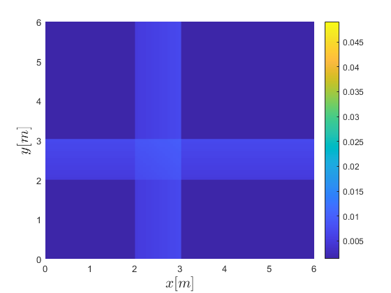
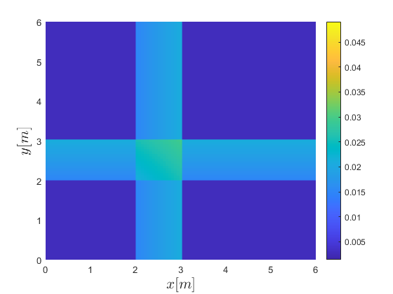
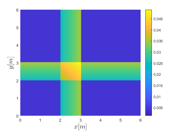
Taking the two-component Gaussian mixtures for illustration, the heatmap of variances of each component of for the and coordinates are shown in Fig. 1. As we can see, the variances in coordinates are larger in the region and . The variances do not change in and coordinates in the experiments. However, we note that the proposed approach is capable of handling cases where the variances may change in all dimensions of the states.
IV-B Reference Distribution Estimation
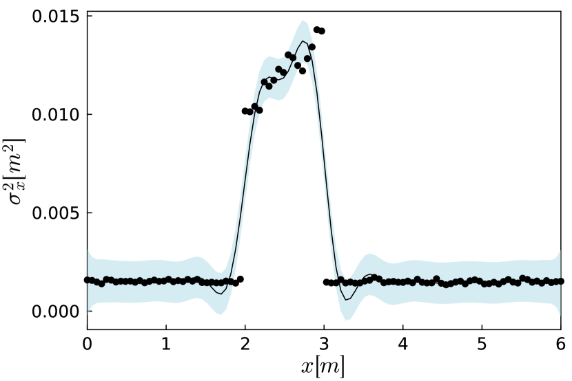
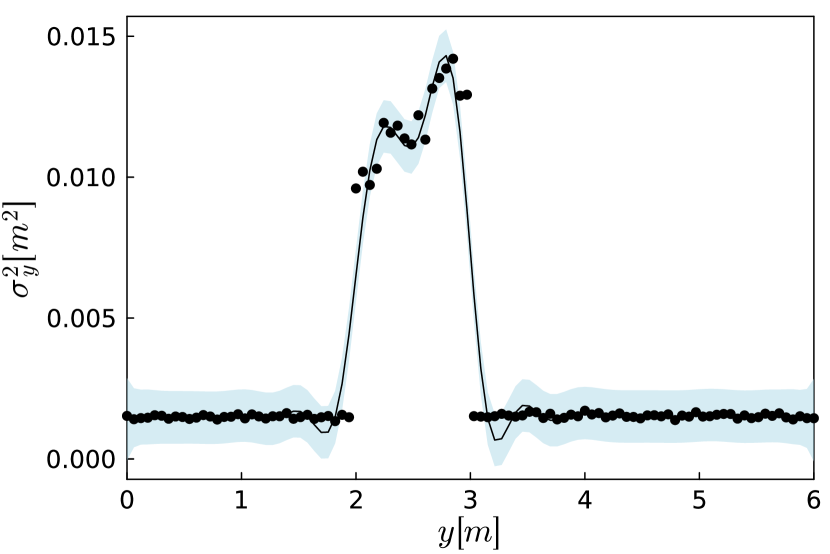
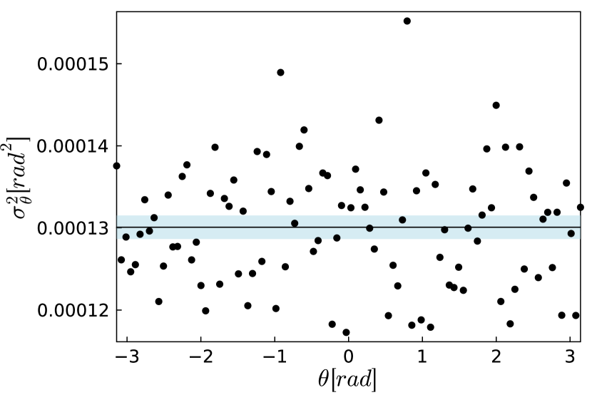
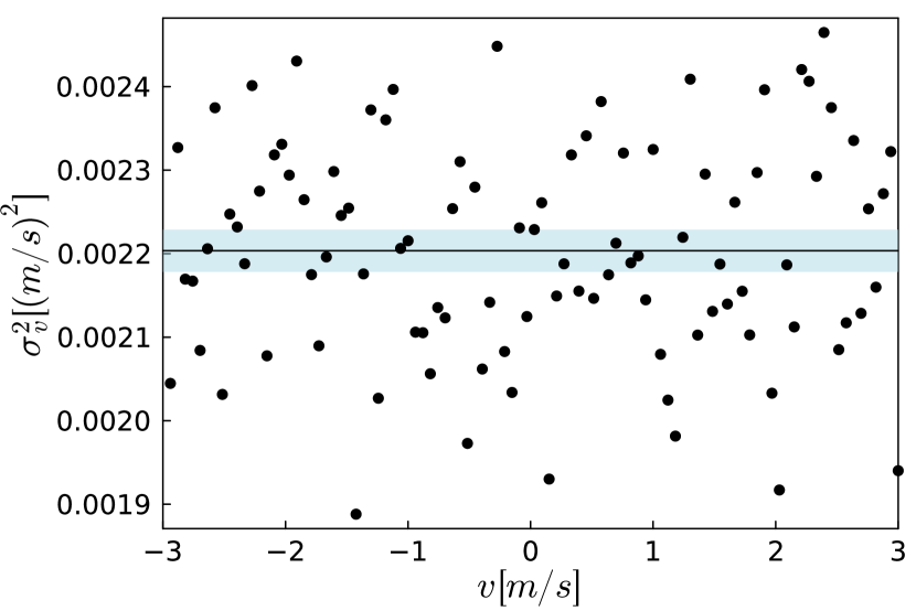
Considering the three different cases of state-dependent noise described above, we trained a Gaussian process (GP) for each dimension of the state to model the reference distribution , as described in Section III-C1. The GP training results of predicting the variances of are shown in Fig. 2 for instance. The black dots represent the variances estimated using MLE for the and coordinates. The line represents the mean, and the shaded area represents the confidence interval. As shown in Fig. 2, the estimated variances in the and coordinates are larger in the region and , which captures the distribution of the true noise . In this specific example, the variances do not change in the and coordinates. The GP-estimated variances in the and coordinates are and , respectively. Combining the variances of each dimension into a diagonal covariance matrix allows us to obtain the state-dependent reference distribution , and the results verify our proposed approach.
IV-C KL Divergence Bound Estimation
In the example of state-dependent noise, we estimated the KL divergence bound using the kNN method. For each horizon, we drew samples from the estimated joint reference distribution and used for the kNN estimation. As a result, we obtained KL divergence bound estimates for three different true noise distributions: for , for , and for .
IV-D Comparison with iLQG
We compared the performance of D3ROC with the risk-neutral control approach iLQG [22]. The robot’s initial state was , with a yaw angle of and velocity of zero. The objective was to navigate to the origin under unknown noise. Both control approaches were executed as a MPC for 22 iterations. To ensure accuracy, we performed 15 runs for each true noise distribution, and the resulting paths of the robot under noise are plotted in Fig. 3. Both control approaches enable the robot to approach the origin. However, D3ROC outperforms iLQG with smaller distances to the origin and more compact paths as the robot gets closer. The plot also reveals D3ROC’s risk-averse behavior, leading the robot to navigate around the region and to avoid areas with higher noise variance. In contrast, iLQG results in more divergent paths, passing through the region and .
Additionally, we present the mean distance between the final position of the robot and the origin for multiple runs under different true noise distributions in Table I. It is evident that the mean final distances and their corresponding standard deviations are smaller under D3ROC compared to iLQG. This finding further supports the effectiveness of our proposed data-driven approach, D3ROC, and demonstrates its ability to successfully handle various true noise distributions.

| Distance | iLQG[m] | D3ROC[m] | iLQG[m] | D3ROC[m] | iLQG[m] | D3ROC[m] |
|---|---|---|---|---|---|---|
| Mean | 0.37 | 0.25 | 0.36 | 0.17 | 0.33 | 0.28 |
| Std | 0.14 | 0.08 | 0.11 | 0.09 | 0.15 | 0.10 |
V Conclusions
In conclusion, this paper presents D3ROC, a data-driven approach that overcomes the limitation of traditional DROC methods requiring known ambiguity sets for noise distribution. We evaluate our approach through a navigation problem for a car-like robot with unknown noise distributions. The numerical results demonstrate that D3ROC achieves smaller mean final distances between the robot and the origin, along with lower corresponding standard deviations, compared to iLQG. Additionally, the risk-averse behavior of D3ROC enables the robot to tend to avoid regions with higher noise variance, whereas iLQG leads to paths passing through such regions. Furthermore, our approach proves effective in handling various noise distributions. Overall, D3ROC offers a promising solution to real-world DROC problems where noise distribution and KL divergence bound are unknown, making the DROC framework more practical and applicable.
References
- [1] OPTIMAL CONTROL OF DISCRETE-TIME SYSTEMS, ch. 2, pp. 19–109. 2012.
- [2] M. Sanjari and H. Karami, “Optimal control strategy of battery-integrated energy system considering load demand uncertainty,” Energy, vol. 210, p. 118525, 2020.
- [3] A. Mesbah, “Stochastic model predictive control with active uncertainty learning: A survey on dual control,” Annual Reviews in Control, vol. 45, pp. 107–117, 2018.
- [4] S. Tang, “Dynamic programming for general linear quadratic optimal stochastic control with random coefficients,” SIAM Journal on Control and Optimization, vol. 53, no. 2, pp. 1082–1106, 2015.
- [5] G. Lee, S. S. Srinivasa, and M. T. Mason, “Gp-ilqg: Data-driven robust optimal control for uncertain nonlinear dynamical systems,” arXiv preprint arXiv:1705.05344, 2017.
- [6] D. Wang, D. Liu, H. Li, B. Luo, and H. Ma, “An approximate optimal control approach for robust stabilization of a class of discrete-time nonlinear systems with uncertainties,” IEEE Transactions on Systems, Man, and Cybernetics: Systems, vol. 46, no. 5, pp. 713–717, 2015.
- [7] H. Nishimura, N. Mehr, A. Gaidon, and M. Schwager, “Rat ilqr: A risk auto-tuning controller to optimally account for stochastic model mismatch,” IEEE Robotics and Automation Letters, vol. 6, no. 2, pp. 763–770, 2021.
- [8] J. Coulson, J. Lygeros, and F. Dörfler, “Distributionally robust chance constrained data-enabled predictive control,” IEEE Transactions on Automatic Control, vol. 67, no. 7, pp. 3289–3304, 2021.
- [9] H. Rahimian and S. Mehrotra, “Distributionally robust optimization: A review,” arXiv preprint arXiv:1908.05659, 2019.
- [10] E. Delage and Y. Ye, “Distributionally robust optimization under moment uncertainty with application to data-driven problems,” Operations research, vol. 58, no. 3, pp. 595–612, 2010.
- [11] E. F. Camacho and C. B. Alba, Model predictive control. Springer science & business media, 2013.
- [12] B. Kouvaritakis and M. Cannon, “Model predictive control,” Switzerland: Springer International Publishing, vol. 38, 2016.
- [13] Z. Hu and L. J. Hong, “Kullback-leibler divergence constrained distributionally robust optimization,” Available at Optimization Online, vol. 1, no. 2, p. 9, 2013.
- [14] Z. Li, W. Wu, B. Zhang, and X. Tai, “Kullback–leibler divergence-based distributionally robust optimisation model for heat pump day-ahead operational schedule to improve pv integration,” IET Generation, Transmission & Distribution, vol. 12, no. 13, pp. 3136–3144, 2018.
- [15] J. Duchi and H. Namkoong, “Learning models with uniform performance via distributionally robust optimization,” arXiv preprint arXiv:1810.08750, 2018.
- [16] E. Schulz, M. Speekenbrink, and A. Krause, “A tutorial on gaussian process regression: Modelling, exploring, and exploiting functions,” Journal of Mathematical Psychology, vol. 85, pp. 1–16, 2018.
- [17] Q. Wang, S. R. Kulkarni, and S. Verdú, “Divergence estimation for multidimensional densities via -nearest-neighbor distances,” IEEE Transactions on Information Theory, vol. 55, no. 5, pp. 2392–2405, 2009.
- [18] Y. Tassa, N. Mansard, and E. Todorov, “Control-limited differential dynamic programming,” in 2014 IEEE International Conference on Robotics and Automation (ICRA), pp. 1168–1175, IEEE, 2014.
- [19] S. Bechtle, Y. Lin, A. Rai, L. Righetti, and F. Meier, “Curious ilqr: Resolving uncertainty in model-based rl,” in Conference on Robot Learning, pp. 162–171, PMLR, 2020.
- [20] D. Nass, B. Belousov, and J. Peters, “Entropic risk measure in policy search,” in 2019 IEEE/RSJ International Conference on Intelligent Robots and Systems (IROS), pp. 1101–1106, IEEE, 2019.
- [21] A. De Luca, G. Oriolo, and C. Samson, “Feedback control of a nonholonomic car-like robot,” Robot motion planning and control, pp. 171–253, 2005.
- [22] M. Athans, “The role and use of the stochastic linear-quadratic-gaussian problem in control system design,” IEEE transactions on automatic control, vol. 16, no. 6, pp. 529–552, 1971.