Federated Virtual Learning on Heterogeneous Data with Local-global Distillation

Abstract

Despite Federated Learning (FL)’s trend for learning machine learning models in a distributed manner, it is susceptible to performance drops when training on heterogeneous data. In addition, FL inevitability faces the challenges of synchronization, efficiency, and privacy. Recently, dataset distillation has been explored in order to improve the efficiency and scalability of FL by creating a smaller, synthetic dataset that retains the performance of a model trained on the local private datasets. We discover that using distilled local datasets can amplify the heterogeneity issue in FL. To address this, we propose a new method, called Federated Virtual Learning on Heterogeneous Data with Local-Global Distillation (FedLGD), which trains FL using a smaller synthetic dataset (referred as virtual data) created through a combination of local and global dataset distillation. Specifically, to handle synchronization and class imbalance, we propose iterative distribution matching to allow clients to have the same amount of balanced local virtual data; to harmonize the domain shifts, we use federated gradient matching to distill global virtual data that are shared with clients without hindering data privacy to rectify heterogeneous local training via enforcing local-global feature similarity. We experiment on both benchmark and real-world datasets that contain heterogeneous data from different sources, and further scale up to an FL scenario that contains large number of clients with heterogeneous and class imbalance data. Our method outperforms state-of-the-art heterogeneous FL algorithms under various settings with a very limited amount of distilled virtual data.

1 Introduction

Federated Learning (FL) [29] has become a popular solution for different institutions to collaboratively train machine learning models without pooling private data together. Typically, it involves a central server and multiple local clients; then the model is trained via aggregation of local network parameter updates on the server side iteratively. FL is widely accepted in many areas, such as computer vision, natural language processing, and medical image analysis [25, 12, 41].

On the one hand, clients with different amounts of data cause asynchronization and affect the efficiency of FL systems. Dataset distillation [39, 5, 46, 44, 45] addresses the issue by only summarizing smaller synthetic datasets from the private local datasets to ensure each client owns the same amount of data. We refer this underexplored strategy as federated virtual learning, as the models are trained from synthetic data [40, 10, 16]. These methods have been found to perform better than model-synchronization-based FL approaches while requiring fewer server-client interactions.

On the other hand, due to different data collection protocols, data from different clients inevitably face heterogeneity problems with domain shift, which means data may not be independent and identically distributed (iid) among clients. Heterogeneous data distribution among clients becomes a key challenge in FL, as aggregating model parameters from non-iid feature distributions suffers from client drift [18] and diverges the global model update[26].

We observe that using locally distilled datasets can amplify the heterogeneity issue. Figure 1 shows the tSNE plots of two different datasets, USPS [31] and SynthDigits [9], each considered as a client. tSNE takes the original and distilled virtual images as input and embeds them into 2D planes. One can observe that the distribution becomes diverse after distillation.

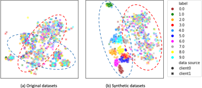
Figure 1: Distilled local datasets can worsen heterogeneity in FL. tSNE plots of (a) original datasets and (b) distilled virtual datasets of USPS (client 0) and SynthDigits (client 1). The two distributions are marked in red and blue. We observe fewer overlapped $\circ$ and $\times$ in (b) compared with (a), indicating higher heterogeneity between two clients after distillation.

To alleviate the problem of data heterogeneity in classical FL settings, two main orthogonal approaches can be taken. Approach 1 aims to minimize the difference between the local and global model parameters to improve convergence [25, 18, 38]. Approach 2 enforces consistency in local embedded features using anchors and regularization loss [37, 47, 42]. The first approach can be easily applied to distilled local datasets, while the second approach has limitations when adapting to federated virtual learning. Specifically, VHL [37] samples global anchors from untrained StyleGAN  [19] suffers performance drop when handling amplified heterogeneity after dataset distillation. Other methods, such as those that rely on external global data [47], or feature sharing from clients [42], are less practical, as they pose greater data privacy risks compared to classical FL settings. Without hindering data privacy, developing strategies following approach 2 for federated virtual learning on heterogeneous data remains open questions on 1) how to set up global anchors for locally distilled datasets and 2) how to select the proper regularization loss(es).

To this end, we propose FedLGD, a federated virtual learning method with local and global distillation. We propose iterative distribution matching in local distillation by comparing the feature distribution of real and synthetic data using an evolving feature extractor. The local distillation results in smaller sets with balanced class distributions, achieving efficiency and synchronization while avoiding class imbalance. FedLGD updates the local model on local distilled synthetic datasets (named local virtual data). We found that training FL with local virtual data can exacerbate heterogeneity in feature space if clients’ data has domain shift (Figure. 1). Therefore, unlike previously proposed federated virtual learning methods that rely solely on local distillation  [10, 40, 16], we also propose a novel and efficient method, federated gradient matching, that integrated well with FL to distill global virtual data as anchors on the server side. This approach aims to alleviate domain shifts among clients by promoting similarity between local and global features. Note that we only share local model parameters w.r.t. distilled data. Thus, the privacy of local original data is preserved. We conclude our contributions as follows:

• This paper focuses on an important but underexplored FL setting in which local models are trained on small distilled datasets, which we refer to as federated virtual learning. We design two effective and efficient dataset distillation methods for FL.

• We are the first to reveal that when datasets are distilled from clients’ data with domain shift, the heterogeneity problem can be exacerbated in the federated virtual learning setting.

• We propose to address the heterogeneity problem by mapping clients to similar features regularized by gradually updated global virtual data using averaged client gradients.

• Through comprehensive experiments on benchmark and real-world datasets, we show that FedLGD outperforms existing state-of-the-art FL algorithms.

2 Related Work

2.1 Dataset Distillation

Data distillation aims to improve data efficiency by distilling the most essential feature in a large-scale dataset (e.g., datasets comprising billions of data points) into a certain terse and high-fidelity dataset. For example, Gradient Matching [46] is proposed to make the deep neural network produce similar gradients for both the terse synthetic images and the original large-scale dataset. Besides, [5] proposes matching the model training trajectory between real and synthetic data to guide the update for distillation. Another popular way of conducting data distillation is through Distribution Matching [45]. This strategy instead, attempts to match the distribution of the smaller synthetic dataset with the original large-scale dataset. It significantly improves the distillation efficiency. Moreover, recent studies have justified that data distillation also preserves privacy [7, 4], which is critical in federated learning. In practice, dataset distillation is used in healthcare for medical data sharing for privacy protection [22]. Other modern data distillation strategies can be found here [33].

2.2 Heterogeneous Federated Learning

FL performance downgrading on non-iid data is a critical challenge. A variety of FL algorithms have been proposed ranging from global aggregation to local optimization to handle this heterogeneous issue. Global aggregation improves the global model exchange process for better unitizing the updated client models to create a powerful server model. FedNova [38] notices an imbalance among different local models caused by different levels of training stage (e.g., certain clients train more epochs than others) and tackles such imbalance by normalizing and scaling the local updates accordingly. Meanwhile, FedAvgM [15] applies the momentum to server model aggregation to stabilize the optimization. Furthermore, there are strategies to refine the server model from learning client models such as FedDF [27] and FedFTG [43]. Local training optimization aims to explore the local objective to tackle the non-iid issue in FL system. FedProx [25] straightly adds $L_{2}$ norm to regularize the client model and previous server model. Scaffold [18] adds the variance reduction term to mitigate the “clients-drift". Also, MOON [24] brings mode-level contrastive learning to maximize the similarity between model representations to stable the local training. There is another line of works [42, 37] proposed to use a global anchor to regularize local training. Global anchor can be either a set of virtual global data or global virtual representations in feature space. However, in [37], the empirical global anchor selection may not be suitable for data from every distribution as they don’t update the anchor according to the training datasets.

2.3 Datasets Distillation for FL

Dataset distillation for FL is an emerging topic that has attracted attention due to its benefit for efficient FL systems. It trains model on distilled synthetic datasets, thus we refer it as federated virtual learning. It can help with FL synchronization and improve training efficiency by condensing every client’s data into a small set. To the best of our knowledge, there are few published works on distillation in FL. Concurrently with our work, some studies [10, 40, 16] distill datasets locally and share the distilled datasets with other clients/servers. Although privacy is protected against currently existing attack models, we consider sharing local distilled data a dangerous move. Furthermore, none of the existing work has addressed the heterogeneity issue.

3 Method

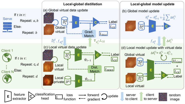
Figure 2: Overview pipeline for FedLGD. We assume $T$ FL rounds will be performed, among which we will define the selected distillation rounds as $\tau\in[T]$ for local-global iteration. For selected rounds ($t\in\tau$), clients will update local models (d) and refine the local virtual data with the latest network parameters (c), while the server uses aggregated gradients from cross-entropy loss ($\mathcal{L_{\rm CE}}$) to update global virtual data (a) and update the global model (b). We term this procedure Iterative Local-global Distillation. For the unselected rounds ($t\in T\backslash\tau$), we perform ordinary FL pipeline on local virtual data with regularization loss ($\mathcal{L_{\rm Con}}$) on global virtual data.

In this section, we will describe the problem setup, introduce the key technical contributions and rationale of the design for FedLGD, and explain the overall training pipeline.

3.1 Setup for Federated Virtual Learning

We start with describing the classical FL setting. Suppose there are $N$ parties who own local datasets ($D_{1},\dots,D_{N}$), and the goal of a classical FL system, such as FedAvg [29], is to train a global model with parameters $\theta$ on the distributed datasets ($D\equiv\bigcup_{i\in[N]}D_{i}$)). The objective function is written as:

$$\mathcal{L}(\theta)=\sum_{i=1}^{N}\frac{|D_{i}|}{|D|}\mathcal{L}_{i}(\theta),$$ (1)

where $\mathcal{L}_{i}(w)$ is the empirical loss of client $i$.

In practice, different clients in FL may have variant amounts of training samples, leading to asynchronized updates. In this work, we focus on a new type of FL training method – federated virtual learning, that trains on distilled datasets for efficiency and synchronization (discussed in Sec.2.3.) Federated virtual learning synthesizes local virtual data $\tilde{D}_{i}$ for client $i$ for $i\in[N]$ and form $\tilde{D}\equiv\bigcup_{i\in[N]}\tilde{D}_{i}$. Typically, $|\tilde{D}_{i}|\ll|{D}_{i}|$ and $|\tilde{D}_{i}|=|\tilde{D}_{j}|$. A basic setup for federated virtual learning is to replace $D_{i}$ with $\tilde{D}_{i}$ in Eq (1), namely FL model is trained on the virtual datasets. As suggested in FedDM [40], the clients should not share gradients w.r.t. the original data for privacy concern.

3.2 Overall Pipeline

The overall pipeline of our proposed method contains three stages, including 1) initialization, 2) iterative local-global distillation, and 3) federated virtual learning. We depict the overview of FedLGD pipeline in Figure 2. However, FL is inevitability affected by several challenges, including synchronization, efficiency, privacy, and heterogeneity. Specifically, we outline FedLGD as follows:

We begin with the initialization of the clients’ local virtual data $\tilde{D}^{c}$ by performing initial rounds of distribution matching (DM) [45]. Meanwhile, the server will initialize global virtual data $\tilde{D}^{g}$ and network parameters $\theta^{g}_{0}$. In this stage, we generate the same amount of class-balanced virtual data for each client and server.

Then, we will refine our local and global virtual data using our proposed local-global distillation strategies in Sec. 3.3.1 and 3.3.2. This step is performed for a few selected iterations (e.g. $\tau=\{0,5,10\}$) to update $\theta$ using $\mathcal{L}_{\rm CE}$ (Eq 3), $\tilde{D}^{g}$ using $\mathcal{L}_{\rm Dist}$ (Eq 5), and $\tilde{D}^{c}$ using $\mathcal{L}_{\rm MMD}$ (Eq 2) in early training epochs. For each selected iterations, the server and clients will update their virtual data for a few distillation steps.

Finally, after refining local and global virtual data $\tilde{D}^{g}$ and $\tilde{D}^{c}$, we continue federated virtual learning in stage 3 on local virtual data $\tilde{D}^{c}$ using $\mathcal{L}_{\rm total}$ (Eq 3), with $\tilde{D}^{g}$ as regularization anchor to calculate $\mathcal{L}_{\rm Con}$ (Eq. 4). We provide implementation details, an algorithm box, and an anonymous link to our code in the Appendix.

3.3 FL with Local-Global Dataset Distillation

3.3.1 Local Data Distillation

Our purpose is to decrease the number of local data to achieve efficient training to meet the following goals. First of all, we hope to synthesize virtual data conditional on class labels to achieve class-balanced virtual datasets. Second, we hope to distill local data that is best suited for the classification task. Last but not least, the process should be efficient due to the limited computational resource locally. To this end, we design Iterative Distribution Matching to fulfill our purpose.

Iterative distribution matching. We aim to gradually improve distillation quality during FL training. To begin with, we split a model into two parts, feature extractor $\psi$ (shown as $E$ in figure 2) and classification head $h$ (shown as $C$ in figure 2). The whole classification model is defined as $f^{\theta}=h\circ\psi$. The high-level idea of distribution matching can be described as follows. Given a feature extractor $\psi:\mathbb{R}^{d}\to\mathbb{R}^{d^{\prime}}$ , we want to generate $\tilde{D}$ so that $P_{\psi}(D)\approx P_{\psi}(\tilde{D})$ where $P$ is the distribution in feature space. To distill local data during FL efficiently that best fits our task, we intend to use the up-to-date server model’s feature extractor as our kernel function to distill better virtual data. Since we can’t obtain ground truth distribution of local data, we utilize empirical maximum mean discrepancy (MMD) [11] as our loss function for local virtual distillation:

$$\mathcal{L}_{\rm MMD}\!=\!\sum_{k}^{K}||\frac{1}{|D^{c}_{k}|}\sum_{i=1}^{|D^{c}_{k}|}\psi^{t}(x_{i})\!-\!\frac{1}{|\tilde{D}^{c,t}_{k}|}\sum_{j=1}^{|\tilde{D}^{c,t}_{k}|}\psi^{t}(\tilde{x}_{j}^{t})||^{2},$$ (2)

where $\psi^{t}$ and $\tilde{D}^{c,t}$ are the server feature extractor and local virtual data from the latest global iteration $t$. Following [46, 45], we apply the differentiable Siamese augmentation on virtual data $\tilde{D}^{c}$. $K$ is the total number of classes, and we sum over MMD loss calculated per class $k\in[K]$. In such a way, we can generate balanced local virtual data by optimizing the same number of virtual data per class.

Although such an efficient distillation strategy is inspired by DM [45], we highlight the key difference that DM uses randomly initialized deep neural networks to extract features, whereas we use trained FL models with task-specific supervised loss. We believe iterative updating on the clients’ data using the up-to-date network parameters can generate better task-specific local virtual data. Our intuition comes from the recent success of the empirical neural tangent kernel for data distribution learning and matching [30, 8]. Especially, the feature extractor of the model trained with FedLGD could obtain feature information from other clients, which further harmonize the domain shift between clients. We apply DM [45] to the baseline FL methods and demonstrate the effectiveness of our proposed iterative strategy in Sec. 4. Furthermore, note that FedLGD only requires a few hundreds of local distillations steps using the local model’s feature distribution, which is more computationally efficient than other bi-level dataset distillation methods [46, 5].

Harmonizing local heterogeneity with global anchors. Data collected in different sites may have different distributions due to different collecting protocols and populations. Such heterogeneity will degrade the performance of FL. Worse yet, we found increased data heterogeneity among clients when federatively training with distilled local virtual data (see Figure 1). We aim to alleviate the dataset shift by adding a regularization term in feature space to our total loss function for local model updating, which is inspired by [37, 20]:

$$\mathcal{L}_{\rm total}=\mathcal{L}_{\rm CE}(\tilde{D}^{g},\tilde{D}^{c};\theta)+\lambda\mathcal{L}_{\rm Con}(\tilde{D}^{g},\tilde{D}^{c}),$$ (3)

and

$$\mathcal{L}_{\rm Con}\!=\!\sum_{i\in I}\frac{-1}{|P(i)|}\!\sum_{p\in P(i)}\!{\rm log}\frac{{\rm exp}(z_{g}\cdot z_{p}/\tau_{temp})}{\sum_{a\in A(i)}{\rm exp}(z_{g}\cdot z_{a}/\tau_{temp})},$$ (4)

where $\mathcal{L}_{\rm CE}$ is the cross-entropy measured on the virtual data, and $\mathcal{L}_{\rm Con}$ is the supervised contrastive loss where $I$ is the collection of all indices, $A(i)$ indicates all the local and global virtual data indices without $i$ (i.e. $A(i)\equiv I\backslash\{i\}$), $z=\psi(x)$ is the output of feature extractor, $P(i)$ represents the set of images belonging to the same class $y_{i}$ without data $i$, and $\tau_{temp}$ is a scalar temperature parameter. In such a way, global virtual data can be served for calibration, where $z_{g}$ is from $\tilde{D}^{g}$ as an anchor, and $z_{p}$ and $z_{a}$ are from $\tilde{D}^{c}$. At this point, a critical problem arises: What global virtual data shall we use?

3.3.2 Global Data Distillation

Here, we provide an affirmative solution to the question of generating global virtual data that can be naturally incorporated into FL pipeline. Although distribution-based matching is efficient, local clients may not share their features due to privacy concerns. Therefore, we propose to leverage local clients’ averaged gradients to distill global virtual data and utilize it in Eq. (4). We term our global data distillation method as Federated Gradient Matching.

Federated gradient matching. The concept of gradient-based dataset distillation is to minimize the distance between gradients from model parameters trained by original data and distilled data. It is usually considered as a learning-to-learn problem because the procedure consists of model updates and distilled data updates. Zhao et al. [46] studies gradient matching in the centralized setting via bi-level optimization that iteratively optimizes the virtual data and model parameters. However, the implementation in [46] is not appropriate for our specific context because there are two fundamental differences in our settings: 1) for model updating, the gradient-distilled dataset is on the server and will not directly optimize the targeted task; 2) for virtual data update, the ‘optimal’ model comes from the optimized local model aggregation. These two steps can naturally be embedded in local model updating and global virtual data distillation from the aggregated local gradients. First, we utilize the distance loss $\mathcal{L}_{Dist}$ [46] for gradient matching:

$$\mathcal{L}_{Dist}=Dist(\bigtriangledown_{\theta}\mathcal{L}_{CE}^{\tilde{D}^{g}}(\theta),\bigtriangledown_{\theta}\mathcal{L}_{CE}^{\tilde{D}^{c}}(\theta))$$ (5)

where $\tilde{D}^{c}$ and $\tilde{D}^{g}$ denote local and global virtual data, $\bigtriangledown_{\theta}\mathcal{L}_{CE}^{\tilde{D}^{c}}$ is the average client gradient. Then, our proposed federated gradient matching optimize as follows:

$$\min_{D^{g}}\mathcal{L}_{Dist}(\theta)\quad\text{subject to}\quad\theta=\frac{1}{N}\theta^{{c_{i}}^{*}},$$

where $\theta^{{c_{i}}^{*}}=\operatorname*{arg\,min}_{\theta}\mathcal{L}_{i}(\tilde{D}^{c})$ is the optimal local model weights of client $i$ at a certain round $t$.

Noting that compared with FedAvg [29], there is no additional client information shared for global distillation. We also note the approach seems similar to the gradient inversion attack [49] but we consider averaged gradients w.r.t. local virtual data, and the method potentially defenses inference attack better (Appendix D.6), which is also implied by [40, 7]. Privacy preservation can be further improved by employing differential privacy [1], but this is not the main focus of our work.

4 Experiment

Table 1: Test accuracy for DIGITS under different images per class (IPC) and model architectures. R and C stand for ResNet18 and ConvNet, respectively, and we set IPC to 10 and 50. There are five clients (MNIST, SVHN, USPS, SynthDigits, and MNIST-M) containing data from different domains. ‘Average’ is the unweighted test accuracy average of all the clients. The best performance under different models is highlighted using bold. The best results on ConvNet are marked in red and in black for ResNet18.

DIGITS		MNIST		SVHN		USPS		SynthDigits		MNIST-M		Average
IPC		10	50	10	50	10	50	10	50	10	50	10	50
FedAvg	R	73.0	92.5	20.5	48.9	83.0	89.7	13.6	28.0	37.8	72.3	45.6	66.3
	C	94.0	96.1	65.9	71.7	91.0	92.9	55.5	69.1	73.2	83.3	75.9	82.6
FedProx	R	72.6	92.5	19.7	48.4	81.5	90.1	13.2	27.9	37.3	67.9	44.8	65.3
	C	93.9	96.1	66.0	71.5	90.9	92.9	55.4	69.0	73.7	83.3	76.0	82.5
FedNova	R	75.5	92.3	17.3	50.6	80.3	90.1	11.4	30.5	38.3	67.9	44.6	66.3
	C	94.2	96.2	65.5	73.1	90.6	93.0	56.2	69.1	74.6	83.7	76.2	83.0
Scaffold	R	75.8	93.4	16.4	53.8	79.3	91.3	11.2	34.2	38.3	70.8	44.2	68.7
	C	94.1	96.3	64.9	73.3	90.6	93.4	56.0	70.1	74.6	84.7	76.0	83.6
MOON	R	15.5	80.4	15.9	14.2	25.0	82.4	10.0	11.5	11.0	35.4	15.5	44.8
	C	85.0	95.5	49.2	70.5	83.4	92.0	31.5	67.2	56.9	82.3	61.2	81.5
VHL	R	87.8	95.9	29.5	67.0	88.0	93.5	18.2	60.7	52.2	85.7	55.1	80.5
	C	95.0	96.9	68.6	75.2	92.2	94.4	60.7	72.3	76.1	83.7	78.5	84.5
FedLGD	R	92.9	96.7	46.9	73.3	89.1	93.9	27.9	72.9	70.8	85.2	65.5	84.4
	C	95.8	97.1	68.2	77.3	92.4	94.6	67.4	78.5	79.4	86.1	80.6	86.7

To evaluate FedLGD, we consider the FL setting in which clients obtain data from different domains while performing the same task. Specifically, we compare with multiple baselines on benchmark datasets DIGITS (Sec. 4.2), where each client has data from completely different open-sourced datasets. The experiment is designed to show that FedLGD can effectively mitigate large domain shifts. Additionally, we evaluate the performance of FedLGD on another benchmark dataset, CIFAR10C [14], which collects data from different corrupts yielding data distribution shift and contains a large number of clients, so that we can investigate varied client sampling in FL. The experiment aims to show FedLGD’s feasibility on large-scale FL environments. We also validate the performance under medical datasets, RETINA, in Appendix. B.

4.1 Training and Evaluation Setup

Model architecture. We conduct the ablation study to explore the effect of different deep neural networks’ performance under FedLGD. Specifically, we adapt ResNet18 [13] and ConvNet [46] in our study. To achieve the optimal performance, we apply the same architecture to perform both the local distillation task and the classification task, as this combination is justified to have the best output [46, 45]. The detailed model architectures are presented in Appendix D.4.

Comparison methods. We compare the performance of downsteam classification tasks using state-of-the-art (SOTA) FL algorithms, FedAvg [29], FedProx [26], FedNova [38], Scaffold [18], MOON [24], and VHL [37]. We directly use local virtual data from our initialization stage for FL methods other than ours. We perform classification on client’s testing set and report the test accuracies.

FL training setup. We use the SGD optimizer with a learning rate of $10^{-2}$ for DIGITS and CIFAR10C. If not specified, our default setting for local model update epochs is 1, total update rounds is 100, the batch size for local training is 32, and the number of virtual data update iterations ($|\tau|$) is 10. The numbers of default virtual data distillation steps for clients and server are set to 100 and 500, respectively. Since we only have a few clients for DIGITS and RETINA experiments, we will select all the clients for each iteration, while the client selection for CIFAR10C experiments will be specified in Sec. 4.3. The experiments are run on NVIDIA GeForce RTX 3090 Graphics cards with PyTorch.

Proper Initialization for Distillation. We propose to initialize the distilled data using statistics from local data to take care of both privacy concerns and model performance. Specifically, each client calculates the statistics of its own data for each class, denoted as $\mu^{c}_{i},\sigma^{c}_{i}$, and then initializes the distillation images per class, $x\sim\mathcal{N}(\mu^{c}_{i},\sigma^{c}_{i})$, where $c$ and $i$ represent each client and categorical label. The server only needs to aggregate the statistics and initializes the virtual data as $x\sim\mathcal{N}(\mu^{g}_{i},\sigma^{g}_{i})$. In this way, no real data is shared with any participant in the FL system. The comparison results using different initialization methods proposed in previous works [46, 45] can be found in Appendix C.

4.2 DIGITS Experiment

Datasets. We use the following datasets for our benchmark experiments: DIGITS = {MNIST [21], SVHN [31], USPS [17], SynthDigits [9], MNIST-M [9]}. Each dataset in DIGITS contains handwritten, real street and synthetic digit images of $0,1,\cdots,9$. As a result, we have 5 clients in the experiments, and image size is $28\times 28$.

Comparison with baselines under various conditions. To validate the effectiveness of FedLGD, we first compare it with the alternative FL methods varying on two important factors: Image-per-class (IPC) and different deep neural network architectures (arch). We use IPC $\in\{10,50\}$ and arch $\in$ { ResNet18(R), ConvNet(C)} to examine the performance of SOTA models and FedLGD using distilled DIGITS. Note that we fix IPC = 10 for global virtual data and vary IPC for local virtual data. Table 1 shows the test accuracies of DIGITS experiments. In addition to testing with original test sets, we also show the unweighted averaged test accuracy. One can observe that for each FL algorithm, ConvNet(C) always has the best performance under all IPCs. The observation is consistent with [45] as more complex architectures may cause over-fitting in training virtual data. It is also shown that using IPC = 50 always outperforms IPC = 10 as expected since more data are available for training. Overall, FedLGD outperforms other SOTA methods, where on average accuracy, FedLGD increases the best test accuracy results among the baseline methods of 2.1% (IPC =10, arch = C), 10.4% (IPC =10, arch = R), 2.2% (IPC = 50, arch = C) and 3.9% (IPC =50, arch = R). VHL [37] is the closest strategy to FedLGD and achieves the best performance among the baseline methods, indicating that the feature alignment solutions are promising for handling heterogeneity in federated virtual learning. However, VHL is still worse than FedLGD, and the performance may result from the differences in synthesizing global virtual data. VHL [37] uses untrained StyleGAN [19] to generate global virtual data without further updating. On the contrary, we update our global virtual data during FL training.

Table 2: Averaged test accuracy for CIFAR10C with ConvNet.

CIFAR10C		FedAvg		FedProx		FedNova		Scaffold		MOON		VHL		FedLGD
IPC		10	50	10	50	10	50	10	50	10	50	10	50	10	50
Client ratio	0.2	27.0	44.9	27.0	44.9	26.7	34.1	27.0	44.9	20.5	31.3	21.8	45.0	32.9	46.8
	0.5	29.8	51.4	29.8	51.4	29.6	45.9	30.6	51.6	23.8	43.2	29.3	51.7	39.5	52.8
	1	33.0	54.9	33.0	54.9	30.0	53.2	33.8	54.5	26.4	51.6	34.4	55.2	47.6	57.4

4.3 CIFAR10C Experiment

Datasets. We conduct real-world FL experiments on CIFAR10C, where, like previous studies [24], we apply Dirichlet distribution with $\alpha=0.5$ to generate 3 partitions on each distorted Cifar10-C [14], resulting in 57 clients each with class imbalanced non-IID datasets. In addition, we apply random client selection with ratio = 0.2, 0.5, and 1 and set image size as $28\times 28$.

Comparison with baselines under different client sampling ratios. The objective of the experiment is to test FedLGD under popular FL questions: class imbalance, large number of clients, different client sample ratios, and data heterogeneity. One benefit of federated virtual learning is that we can easily handle class imbalance by distilling the same number (IPC) of virtual data. We will vary IPC and fix the model architecture to ConvNet since it is validated that ConvNet yields better performance in virtual training [46, 45]. One can observe from Table 2 that FedLGD consistently achieves the best performance under different IPC and client sampling ratios. We would like to point out that when IPC=10, the performance boosts are significant, which indicates that FedLGD is well-suited for FL conditions when there is a large group of clients and each of them has a limited number of data.

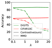
(a) Comparison of Reg. loss

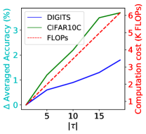
(b) Vary $|\tau|$

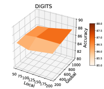
(c) Vary steps

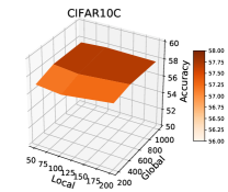
(d) Vary steps

Figure 3: (a) Comparison between different regularization losses and their weighting in total loss ($\lambda$). One can observe that supervised contrastive loss gives us better and more stable performance with different coefficient choices. (b) The trade-off between $|\tau|$ and computation cost. One can observe that the model performance improves with the increasing $|\tau|$, which is a trade-off between computation cost and model performance. Vary data updating steps for (c) DIGITS and (d) CIFAR10C. One can observe that FedLGD yields consistent performance, and the accuracy tends to improve with an increasing number of local and global steps.

4.4 Ablation studies for FedLGD

The success of FedLGD relies on the novel design of local-global data distillation, where the selection of regularization loss and the number of iterations for data distillation plays a key role. In this section, we study the choice of regularization loss and its weighting ($\lambda$) in the total loss function. Recall that among the total FL training epochs, we perform local-global distillation on the selected $\tau$ iterations, and within each selected iteration, the server and clients will perform data updating for some pre-defined steps. The effect of local-global distillation iterations and data updating steps will also be discussed. We also perform additional ablation studies such as computation cost and communication overhead in Appendix C.

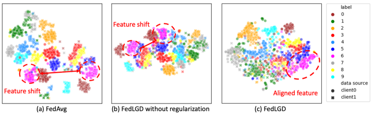
Figure 4: tSNE plots on feature space for FedAvg, FedLGD without regularization, and FedLGD. One can observe regularizing training with our global virtual data can rectify feature shift among different clients.

Effect of regularization loss. FedLGD uses supervised contrastive loss $\mathcal{L}_{\rm Con}$ as a regularization term to encourage local and global virtual data embedding into a similar feature space. To demonstrate the effectiveness of the regularization term in FedLGD, we perform ablation studies to replace $\mathcal{L}_{\rm Con}$ with an alternative distribution similarity measurement, MMD loss, with different $\lambda$’s ranging from 0.1 to 20. Figure 3a shows the average test accuracy. Using supervised contrastive loss gives us better and more stable performance with different coefficient choices.

To explain the effect of our proposed regularization loss on feature representations, we embed the latent features before fully-connected layers to a 2D space using tSNE [28] shown in Figure 4. For the model trained with FedAvg (Figure 4(a)), features from two clients ($\times$ and $\circ$) are closer to their own distribution regardless of the labels (colors). In Figure 4(b), we perform virtual FL training but without the regularization term (Eq. 4). Figure 4(c) shows FedLGD, and one can observe that data from different clients with the same label are grouped together. This indicates that our regularization with global virtual data is useful for learning homogeneous feature representations.

Analysis of distillation iterations ($|\tau|$). Figure 3b shows the improved averaged test accuracy if we increase the number of distillation iterations with FedLGD. The base accuracy for DIGITS and CIFAR10C are 85.8 and 55.2, respectively. We fix local and global update steps to 100 and 500, and the selected iterations ($\tau$) are defined as arithmetic sequences with $d=5$ (i.e., $\tau=\{0,5,...\}$). One can observe that the model performance improves with the increasing $|\tau|$. This is because we obtain better virtual data with more local-global distillation iterations, which is a trade-off between computation cost and model performance. We select $|\tau|=10$ for efficiency trade-off.

Robustness on virtual data update steps. In Figure 3c and Figure 3d, we fix $|\tau|=10$, and vary (local, global) data updating steps. One can observe that FedLGD yields stable performance, and the accuracy slightly improves with an increasing number of local and global steps. Nevertheless, the results are all the best when comparing with the baselines. It is also worth noting that there is still trade-off between steps and computation cost (See Appendix).

5 Conclusion

In this paper, we introduce a new approach for FL, called FedLGD. It utilizes virtual data on both client and server sides to train FL models. We are the first to reveal that FL on local virtual data can increase heterogeneity. Furthermore, we propose iterative distribution matching and federated gradient matching to iteratively update local and global virtual data, and apply global virtual regularization to effectively harmonize domain shift. Our experiments on benchmark and real medical datasets show that FedLGD outperforms current state-of-the-art methods in heterogeneous settings. Furthermore, FedLGD can be combined with other heterogenous FL methods such as FedProx [26] and Scaffold [18] to further improve its performance. The potential limitation lies in the additional communication and computation cost in data distillation, but we show that the trade-off is acceptable and can be mitigated by decreasing distillation iterations and steps. Our future direction will be investigating privacy-preserving data generation. We believe that this work sheds light on how to effectively mitigate data heterogeneity from a dataset distillation perspective and will inspire future work to enhance FL performance, privacy, and efficiency.

Road Map of Appendix Our appendix is organized into five sections. The notation table is in Appendix A, which contains the mathematical notation and Algorithm 1, which outlines the pipeline of FedLGD. Appendix B shows the results for RETINA, a real-world medical dataset. Appendix C provides a list of ablation studies to analyze FedLGD, including computation cost, communication overhead, convergence rate, and hyper-parameter choices. Appendix D lists the details of our experiments: D.1 visualizes the original sample images used in our experiments; D.2 visualizes the local and global distilled images; D.3 shows the pixel histogram for the DIGITS and RETINA datasets for visualizing the heterogeneity of them; D.4 shows the model architectures that we used in the experiments; D.5 contains the hyper-parameters that we used to conduct all experiments;  D.6 provides experiments and analysis for the privacy of FedLGD through membership inference attack. Finally, Appendix E provides a detailed literature review and implementation of the state-of-the-art heterogeneous FL strategies. Our code and model checkpoints are available in this anonymous link: https://drive.google.com/drive/folders/1Hpy8kgPtxC_NMqK6eALwukFZJB7yf8Vl?usp=sharing.

Appendix A Notation Table

Table 3: Important notations used in the paper.

Notations	Description
$d$	input dimension
$d^{\prime}$	feature dimension
$f^{\theta}$	global model
$\theta$	model parameters
$\psi$	feature extractor
$h$	projection head
$D^{g},D^{c}$	original global and local data
$\tilde{D}^{g},\tilde{D}^{c}$	global and local synthetic data
$\tilde{f}^{g},\tilde{f}^{c}$	features of global and local synthetic data
$\mathcal{L_{\rm total}}$	total loss function for virtual federated training
$\mathcal{L_{\rm CE}}$	cross-entropy loss
$\mathcal{L_{\rm Dist}}$	Distance loss for gradient matching
$\mathcal{L_{\rm MMD}}$	MMD loss for distribution matching
$\mathcal{L_{\rm Con}}$	Contrastive loss for local training regularization
$\lambda$	coefficient for local training regularization term
$T$	total training iterations
$T^{\rm c}_{\rm D}$	local data updating iterations for each call
$T^{\rm g}_{\rm D}$	global data updating iterations for each call
$\tau$	local global distillation iterations

Algorithm 1 Federated Virtual Learning with Local-global Distillation

$f^{\theta}$: Model, $\psi^{\theta}$: Feature extractor, $\theta$: Model parameters, $\tilde{D}$: Virtual data, $D$: Original data, $\mathcal{L}$: Losses, $G$: Gradients.

Distillation Functions:

$\tilde{D}^{\rm c}\leftarrow{\rm DistributionMatch}(D^{\rm c},f^{\theta})$

$\tilde{D}^{\rm c}_{\rm t}\leftarrow{\rm IterativeDistributionMatch}(\tilde{D}^{\rm c}_{\rm t-1},f^{\theta}_{\rm t})$

$\tilde{D}^{\rm g}_{\rm t+1}\leftarrow{\rm FederatedGradientMatch}(\tilde{D}^{\rm g}_{\rm t},G^{\rm g}_{\rm t})$

Initialization:

$\tilde{D}^{\rm c}_{\rm 0}\leftarrow{\rm DistributionMatch}(D^{\rm c}_{\rm rand},f^{\theta}_{\rm rand})$ $\triangleright$ Distilled local data for virtual FL training

FedLGD Pipeline:

for $t=1,\dots,T$ do

     Clients:

     for each selected Client do

         if $t\in\tau$ then $\triangleright$ Local-global distillation

              $\tilde{D}^{\rm c}_{\rm t}\leftarrow{\rm IterativeDistributionMatch}(\tilde{D}^{\rm c}_{\rm t-1},f^{\theta}_{\rm t})$

              $G^{\rm c}_{\rm t}\leftarrow\nabla_{\theta}\mathcal{L}_{\rm CE}(\tilde{D}^{\rm c}_{\rm t},f^{\theta}_{\rm t})$

         else

              $\tilde{D}^{\rm c}_{\rm t}\leftarrow\tilde{D}^{\rm c}_{\rm t-1}$

              $G^{\rm c}_{\rm t}\leftarrow\nabla_{\theta}\left(\mathcal{L}_{\rm CE}(\tilde{D}^{\rm c}_{\rm t},f^{\theta}_{\rm t})+\lambda\mathcal{L}_{\rm CON}(\psi^{\theta}_{\rm t}(\tilde{D}^{\rm g}_{\rm t}),\psi^{\theta}_{\rm t}(\tilde{D}^{\rm c}_{\rm t}))\right)$

         end if

         Uploads $G^{\rm c}_{t}$ to Server

     end for

     Server:

     $G^{\rm g}_{\rm t}\leftarrow{\rm Aggregate}(G^{\rm 1}_{\rm t},...,G^{\rm c}_{\rm t})$

     if $t\in\tau$ then $\triangleright$ Local-global distillation

         $\tilde{D}^{\rm g}_{\rm t+1}\leftarrow{\rm FederatedGradientMatch}(\tilde{D}^{\rm g}_{\rm t},G^{\rm g}_{\rm t})$

         Send $\tilde{D}^{\rm g}_{\rm t+1}$ to Clients

     end if

     $f^{\theta}_{\rm t+1}\leftarrow{\rm ModelUpdate}(G^{\rm g}_{\rm t},f^{\theta}_{\rm t})$

     Send $f^{\theta}_{\rm t+1}$ to Clients

end for

Appendix B Experiment Results on Real-world Dataset

Table 4: Test accuracy for RETINA experiments under different model architectures and IPC=10. R and C stand for ResNet18 and ConvNet, respectively. We have 4 clients: Drishti(D), Acrima(A), Rim(Ri), and Refuge(Re), respectively. We also show the average test accuracy (Avg). The best results on ConvNet are marked in red and in bold for ResNet18. The same accuracy for different methods is due to the limited number of testing samples.

RETINA		D	A	Ri	Re	Avg
FedAvg	R	31.6	71.0	52.0	78.5	58.3
	C	69.4	84.0	88.0	86.5	82.0
FedProx	R	31.6	70.0	52.0	78.5	58.0
	C	68.4	84.0	88.0	86.5	81.7
FedNova	R	31.6	71.0	52.0	78.5	58.3
	C	68.4	84.0	88.0	86.5	81.7
Scaffold	R	31.6	73.0	49.0	78.5	58.0
	C	68.4	84.0	88.0	86.5	81.7
MOON	R	42.1	71.0	57.0	70.0	60.0
	C	57.9	72.0	76.0	85.0	72.7
VHL	R	47.4	62.0	50.0	76.5	59.0
	C	68.4	78.0	81.0	87.0	78.6
FedLGD	R	57.9	75.0	59.0	77.0	67.2
	C	78.9	86.0	88.0	87.5	85.1

Dataset. For medical dataset, we use the retina image datasets, RETINA = {Drishti [36], Acrima[6], Rim [2], Refuge [32]}, where each dataset contains retina images from different stations with image size $96\times 96$, thus forming four clients in FL. We perform binary classification to identify Glaucomatous and Normal. Example images and distributions can be found in Appendix D.3. Each client has a held-out testing set. In the following experiments, we will use the distilled local virtual training sets for training and test the models on the original testing sets. The sample population statistics for both experiments are available in Table 12 and Table 14 in Appendix D.5.

Comparison with baselines. The results for RETINA experiments are shown in Table 4, where D, A, Ri, Re represent Drishti, Acrima, Rim, and Refuge datasets. We only set IPC=10 for this experiment as clients in RETINA contain much fewer data points. The learning rate is set to 0.001. The same as in the previous experiment, we vary arch $\in$ { ConvNet, ResNet18}. Similarly, ConvNet shows the best performance among architectures, and FedLGD has the best performance compared to the other methods w.r.t the unweighted averaged accuracy (Avg) among clients. To be precise, FedLGD increases unweighted averaged test accuracy for 3.1%(versus the best baseline) on ConvNet and 7.2%(versus the best baseline) on ResNet18, respectively. The same accuracy for different methods is due to the limited number of testing samples. We conjecture the reason why VHL [37] has lower performance improvement in RETINA experiments is that this dataset is in higher dimensional and clinical diagnosis evidence on fine-grained details, e.g., cup-to-disc ratio and disc rim integrity [34]. Therefore, it is difficult for untrained StyleGAN [19] to serve as anchor for this kind of larger images.

Appendix C Additional Results and Ablation Studies for FedLGD

C.1 Different random seeds

To show the consistent performance of FedLGD, we repeat the experiments for DIGITS, CIFAR10C, and RETINA with three random seeds, and report the validation loss and accuracy curves in Figure 5 and 6 (The standard deviations of the curves are plotted as shadows.). We use ConvNet for all the experiments. IPC is set to 50 for CIFAR10C and DIGITS; 10 for RETINA. We use the default hyperparameters for each dataset, and only report FedAvg, FedProx, Scaffold, VHL, which achieves the best performance among baseline as indicated in Table 1, 2, and 4 for clear visualization. One can observe that FedLGD has faster convergence rate and results in optimal performances compared to other baseline methods.

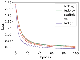
(a)

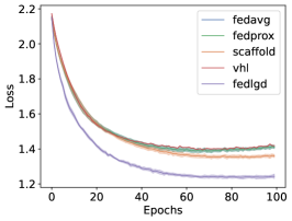
(b)

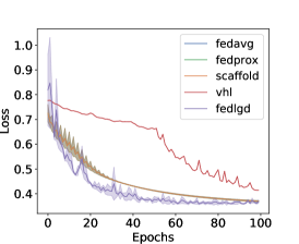
(c)

Figure 5: Averaged testing loss for (a) DIGITS with IPC = 50, (b) CIFAR10C with IPC = 50, and (c) RETINA with IPC = 10 experiments.

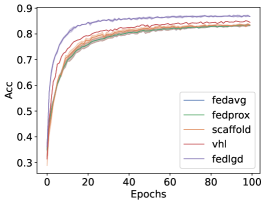
(a)

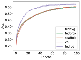
(b)

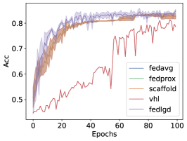
(c)

Figure 6: Averaged testing accuracy for (a) DIGITS with IPC = 50, (b) CIFAR10C with IPC = 50, and (c) RETINA with IPC = 10 experiments.

C.2 Different heterogeniety levels of label shift

In the experiment presented in Sec 4.3, we study FedLGD under both label and domain shifts, where labels are sampled from Dirichlet distribution. To ensure dataset distillation performance, we ensure that each class at least has 100 samples per client, thus setting the coefficient of Dirichlet distribution $\alpha=2$ to simulate the worst case of label heterogeneity that meets the quality dataset distillation requirement . Here, we show the performance with a less heterogeneity level ($\alpha=5$) while keeping the other settings the same as those in Sec.4.3. The results are shown in Table 5. As we expect, the performance drop when the heterogeneity level increases ($\alpha$ decreases). One can observe that when heterogeneity increases, FedLGD’s performance drop less except for VHL. We conjecture that VHL yields similar test accuracy for $\alpha=2$ and $\alpha=5$ is that it uses fixed global virtual data so that the effectiveness of regularization loss does not improve much even if the heterogeneity level is decreased. Nevertheless, FedLGD consistently outperforms all the baseline methods.

Table 5: Comparison of different $\alpha$ for Drichilet distribution on CIFAR10C.

$\alpha$	FedAvg [29]	FedProx [26]	FedNova [38]	Scaffold [18]	MOON [24]	VHL [37]	FedLGD
2	54.9	54.9	53.2	54.5	51.6	55.2	57.4
5	55.4	55.4	55.4	55.6	51.1	55.4	58.1

Table 6: Computation cost for each epoch. Nc and Ns stand for the number of updating iteration for local and global virtual data, and we defaultly set as $100$ and $500$, respectively. Note that we only set $|\tau|=10$ iterations, which is a relatively small number compare to total epochs(100).

Dataset	Vanilla FedAvg	FedLGD(iters $\in$ $\tau$)	FedLGD(iters $\notin$ $\tau$)	FedLGD(server)
DIGITS	238K	2.7K + 3.4K $\times$ Nc	4.8K	2.9K $\times$ Ns
CIFAR10C	53M	2.7K + 3.4K $\times$ Nc	4.8K	2.9K $\times$ Ns
RETINA	1.76M	0.7K + 0.9K $\times$ Nc	1K	0.9K $\times$ Ns

C.3 Computation Cost

Computation cost for DIGITS experiment on each epoch can be found in Table 7. Nc and Ns stand for the number of updating iterations for local and global virtual data, and as default, we it set as $100$ and $500$, respectively. The computation costs for FedLGD in DIGITS and CIFAR10C are identical since we used virtual data with fixed size and number for training. Plugging in the number, clients only need to operate 3.9M FLOPs for total 100 training epochs with $\tau=10$ (our default setting), which is significantly smaller than vanilla FedAvg using original data (23.8M and 5,300M for DIGITS and CIFAR10C, respectively.).

Table 7: Communication overhead for each epoch. Note that the IPC for our global virtual data is 10, and the clients only need to download it for $|\tau|=10$ times.

Image size	ConvNet	ResNet18	Global virtual data
28 $\times$ 28	311K	11M	23K $\times$ IPC
96 $\times$ 96	336K	13M	55K $\times$ IPC

C.4 Communication Overhead

The communication overhead for each epoch in DIGITS and CIFAR10C experiments are identical since we use same architectures and size of global virtual data (Table. 7 28 $\times$ 28). The analysis of RETINA is shown in row 96 $\times$ 96. Note that the IPC for our global virtual data is 10, and the clients only need to download it for $|\tau|$ times. Although FedLGD requires clients to download additional data which is almost double the original Bytes (311K + 230K), we would like to point out that this only happens $|\tau|=10$ times, which is a relatively small number compared to total FL training iterations.

C.5 Analysis of batch size

Batch size is another factor for training the FL model and our distilled data. We vary the batch size $\in\{8,16,32,64\}$ to train models for CIFAR10C with the fixed default learning rate. We show the effect of batch size in Table 8 reported on average testing accuracy. One can observe that the performance is slightly better with moderately smaller batch size which might due to two reasons: 1) more frequent model update locally; and 2) larger model update provides larger gradients, and FedLGD can benefit from the large gradients to distill higher quality virtual data. Overall, the results are generally stable with different batch size choices.

Table 8: Varying batch size in FedLGD on CIFAR10C. We report the unweighted accuracy. One can observe that the performance increases when the batch size decreases.

Batch Size	8	16	32	64
CIFAR10C	59.5	58.3	57.4	56.0

C.6 Analysis of Local Epoch

Aggregating at different frequencies is known as an important factor that affects FL behavior. Here, we vary the local epoch $\in\{1,2,5\}$ to train all baseline models on CIFAR10C. Figure 7 shows the result of test accuracy under different epochs. One can observe that as the local epoch increases, the performance of FedLGD would drop a little bit. This is because doing gradient matching requires the model to be trained to an intermediate level, and if local epochs increase, the loss of DIGITS models will drop significantly. However, FedLGD still consistently outperforms the baseline methods. As our future work, we will investigate the tuning of the learning rate in the early training stage to alleviate the effect.

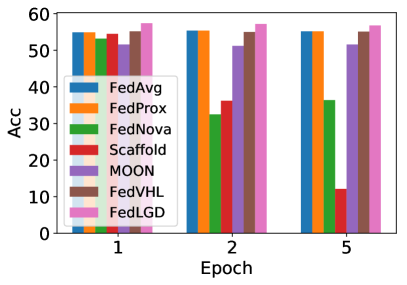
Figure 7: Comparison of model performances under different local epochs with CIFAR10C.

C.7 Different Initialization for Virtual Images

To validate our proposed initialization for virtual images has the best trade-off between privacy and efficacy, we compare our test accuracy with the models trained with synthetic images initialized by random noise and real images in Table 9. To show the effect of initialization under large domain shift, we run experiments on DIGITS dataset. One can observe that our method which utilizes the statistics ($\mu_{i},\sigma_{i}$) of local clients as initialization outperforms random noise initialization. Although our performance is slightly worse than the initialization that uses real images from clients, we do not ask the clients to share real images to the server which is more privacy-preserving.

Table 9: Comparison of different initialization for synthetic images DIGITS

CIFAR10C	MNIST	SVHN	USPS	SynthDigits	MNIST-M	Average
Noise ($\mathcal{N}(0,1)$)	96.3	75.9	93.3	72.0	83.7	84.2
Ours ($\mathcal{N}(\mu_{i},\sigma_{i})$)	97.1	77.3	94.6	78.5	86.1	86.7
Real images	97.7	78.8	94.2	82.4	89.5	88.5

Appendix D Experimental details

D.1 Visualization of the original images

D.1.1 Digits dataset

(a)

(b)

(c)

(d)

(e)

Figure 8: Visualization of the original digits dataset. (a) visualized the MNIST client; (b) visualized the SVHN client; (c) visualized the USPS client; (d) visualized the SynthDigits client; (e) visualized the MNIST-M client.

D.1.2 Retina dataset

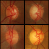
(a)

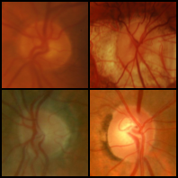
(b)

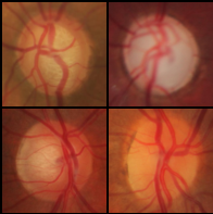
(c)

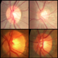
(d)

Figure 9: Visualization of the original retina dataset. (a) visualized the Drishti client; (b) visualized the Acrima client; (c) visualized the Rim client; (d) visualized the Refuge client.

D.1.3 Cifar10C dataset

(a)

(b)

(c)

(d)

(e)

(f)

Figure 10: Visualization of the original CIFAR10C. Sampled images from the first six clients.

D.2 Visualization of our distilled global and local images

D.2.1 Digits dataset

(a)

(b)

(c)

(d)

(e)

(f)

Figure 11: Visualization of the global and local distilled images from the digits dataset. (a) visualized the MNIST client; (b) visualized the SVHN client; (c) visualized the USPS client; (d) visualized the SynthDigits client; (e) visualized the MNIST-M client; (f) visualized the server distilled data.

D.2.2 Retina dataset

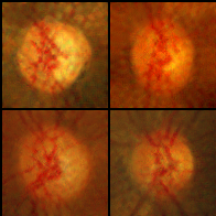
(a)

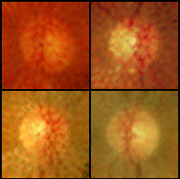
(b)

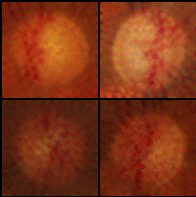
(c)

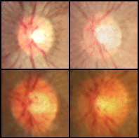
(d)

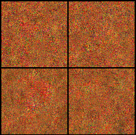
(e)

Figure 12: Visualization of the global and local distilled images from retina dataset. (a) visualized the Drishti client; (b) visualized the Acrima client; (c) visualized the Rim client; (d) visualized the Refuge client; (e) visualized the server distilled data.

D.2.3 Cifar10C dataset

(a)

(b)

(c)

(d)

(e)

(f)

(g)

Figure 13: (a)-(f) visualizes the distailled images for the first six clients of CIFAR10C. (g) visualizes the global distilled images.

D.3 Visualization of the heterogeneity of the datasets

D.3.1 Digits dataset

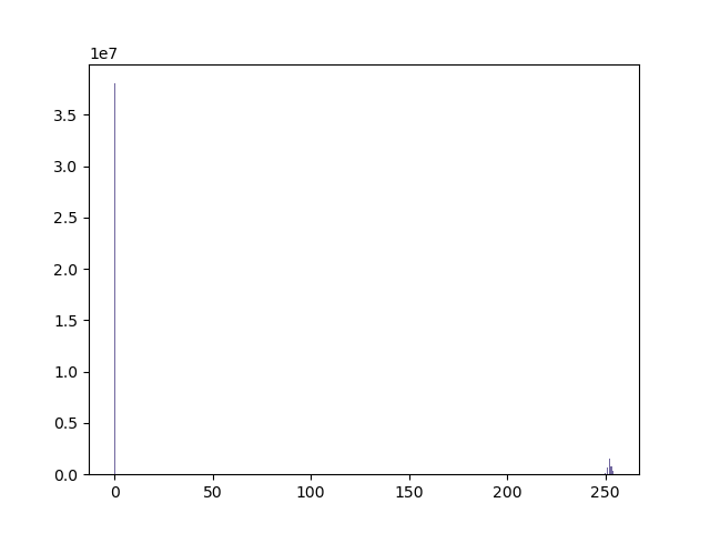
(a) MNIST

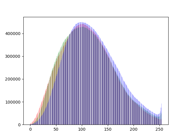
(b) SVHN

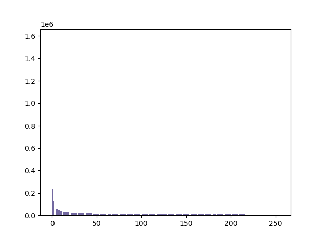
(c) USPS

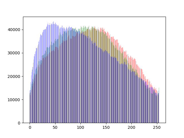
(d) SynthDigits

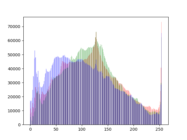
(e) MNIST-M

Figure 14: Histogram for the frequency of each RGB value in original DIGITS. The red bar represents the count for R; the green bar represents the frequency of each pixel for G; the blue bar represents the frequency of each pixel for B. One can observe the distributions are very different. Note that figure (a) and figure (c) are both greyscale images with most pixels lying in 0 and 255.

D.3.2 Retina dataset

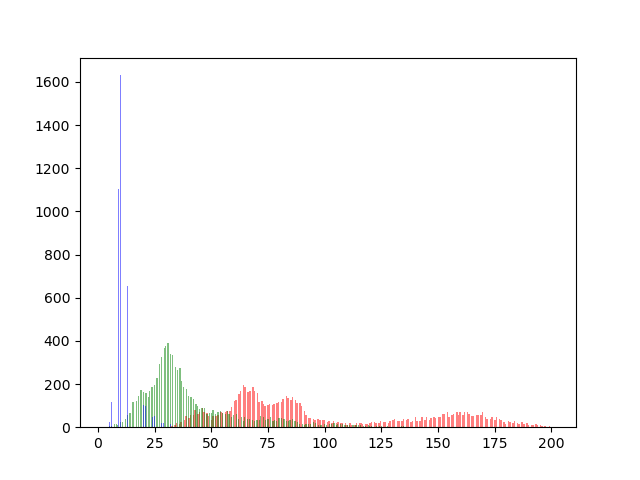
(a) Drishti

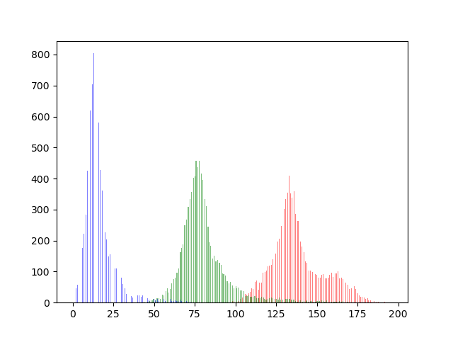
(b) Acrima

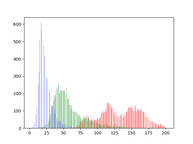
(c) RIM

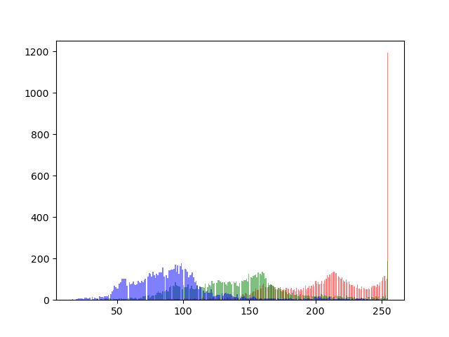
(d) REFUGE

Figure 15: Histogram for the frequency of each RGB value in original RETINA. The red bar represents the count for R; the green bar represents the frequency of each pixel for G; the blue bar represents the frequency of each pixel for B.

D.3.3 CIFAR10C dataset

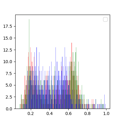
(a)

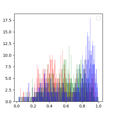
(b)

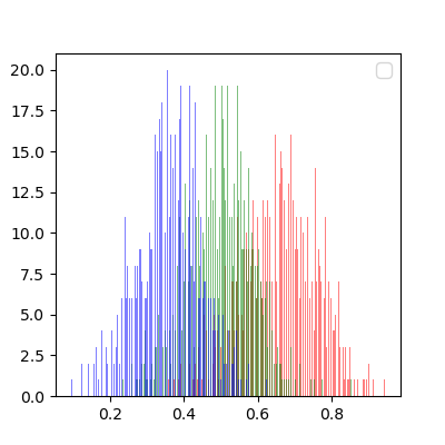
(c)

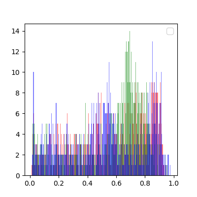
(d)

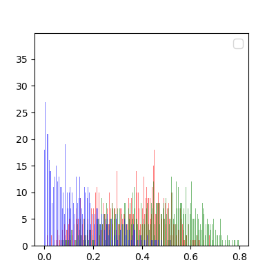
(e)

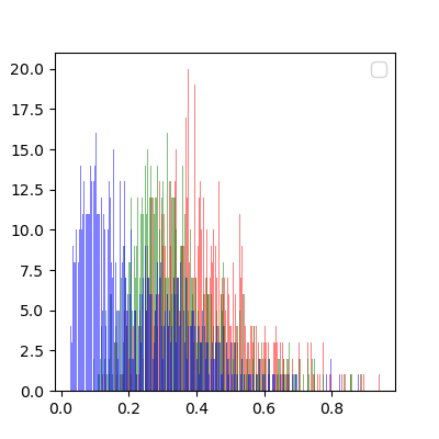
(f)

Figure 16: Histogram for the frequency of each RGB value in the first six clients of original CIFAR10C. The red bar represents the count for R; the green bar represents the frequency of each pixel for G; the blue bar represents the frequency of each pixel for B.

D.4 Model architecture

For our benchmark experiments, we use ConvNet to both distill the images and train the classifier.

Table 10: ResNet 18 architecture. For the convolutional layer (Conv2D), we list parameters with a sequence of input and output dimensions, kernel size, stride, and padding. For the max pooling layer (MaxPool2D), we list kernel and stride. For a fully connected layer (FC), we list input and output dimensions. For the BatchNormalization layer (BN), we list the channel dimension.

Layer	Details
1	Conv2D(3, 64, 7, 2, 3), BN(64), ReLU
2	Conv2D(64, 64, 3, 1, 1), BN(64), ReLU
3	Conv2D(64, 64, 3, 1, 1), BN(64)
4	Conv2D(64, 64, 3, 1, 1), BN(64), ReLU
5	Conv2D(64, 64, 3, 1, 1), BN(64)
6	Conv2D(64, 128, 3, 2, 1), BN(128), ReLU
7	Conv2D(128, 128, 3, 1, 1), BN(64)
8	Conv2D(64, 128, 1, 2, 0), BN(128)
9	Conv2D(128, 128, 3, 1, 1), BN(128), ReLU
10	Conv2D(128, 128, 3, 1, 1), BN(64)
11	Conv2D(128, 256, 3, 2, 1), BN(128), ReLU
12	Conv2D(256, 256, 3, 1, 1), BN(64)
13	Conv2D(128, 256, 1, 2, 0), BN(128)
14	Conv2D(256, 256, 3, 1, 1), BN(128), ReLU
15	Conv2D(256, 256, 3, 1, 1), BN(64)
16	Conv2D(256, 512, 3, 2, 1), BN(512), ReLU
17	Conv2D(512, 512, 3, 1, 1), BN(512)
18	Conv2D(256, 512, 1, 2, 0), BN(512)
19	Conv2D(512, 512, 3, 1, 1), BN(512), ReLU
20	Conv2D(512, 512, 3, 1, 1), BN(512)
21	AvgPool2D
22	FC(512, num_class)

Table 11: ConvNet architecture. For the convolutional layer (Conv2D), we list parameters with a sequence of input and output dimensions, kernel size, stride, and padding. For the max pooling layer (MaxPool2D), we list kernel and stride. For a fully connected layer (FC), we list the input and output dimensions. For the GroupNormalization layer (GN), we list the channel dimension.

Layer	Details
1	Conv2D(3, 128, 3, 1, 1), GN(128), ReLU, AvgPool2d(2,2,0)
2	Conv2D(128, 118, 3, 1, 1), GN(128), ReLU, AvgPool2d(2,2,0)
3	Conv2D(128, 128, 3, 1, 1), GN(128), ReLU, AvgPool2d(2,2,0)
4	FC(1152, num_class)

D.5 Training details

We provide detailed settings for experiments conducted in Table 12 for DIGITS, Table 13 for CIFAR10C, and Table 14 for RETINA.

Table 12: DIGITS settings for all federated learning, including the number of training and testing examples, and local update epochs. Image per class is the number of distilled images used for distribution matching only in FedLGD.

DataSets	MNIST	SVHN	USPS	SynthDigits	MNIST-M
Number of clients	1	1	1	1	1
Number of Training Samples	60000	73257	7291	10000	10331
Number of Testing Samples	10000	26032	2007	2000	209
Image per Class	10,50	10,50	10,50	10,50	10,50
Local Update Epochs	1,2,5	1,2,5	1,2,5	1,2,5	1,2,5
Local Distillation Update Epochs	50, 100, 200	50, 100, 200	50, 100, 200	50, 100, 200	50, 100, 200
global Distillation Update Epochs	200, 500, 1000	200, 500, 1000	200, 500, 1000	200, 500, 1000	200, 500, 1000
$\lambda$	10	10	10	10	10

Table 13: CIFAR10C settings for all federated learning, including the client ratio for training and testing examples, and local update epochs. Image per class is the number of distilled images used for distribution matching only in FedLGD.

$\alpha$	2	5
Number of clients	57	57
Averaged Number of Training Samples	21790	15000
Standard Deviation of of Training Samples	6753	1453
Averaged Number of Testing Samples	2419	1666
Standard Deviation of Number of Testing Samples	742	165
Image per Class	10,50	10,50
Local Update Epochs	1,2,5	1,2,5
Local Distillation Update Epochs	50, 100, 200	50, 100, 200
global Distillation Update Epochs	200, 500, 1000	200, 500, 1000
$\lambda$	1	1

Table 14: RETINA settings for all federated learning, including the number of training and testing examples and local update epochs. Image per class is the number of distilled images used for distribution matching only in FedLGD.

Datasets	Drishti	Acrima	RIM	Refuge
Number of clients	1	1	1	1
Number of Training Samples	82	605	385	1000
Number of Testing Samples	19	100	100	200
Image per class	10	10	10	10
Local Distillation Update Epochs	100	100	100	100
global Distillation Update Epochs	500	500	500	500
$\lambda$	0.1	0.1	0.1	0.1

D.6 Membership Inference Attack

Studies show that neural networks are prone to suffer from several privacy attacks such as Membership Inference Attacks (MIA) [35]. In MIA, the attackers have a list of query data, and the purpose is to determine whether the query data belongs to the original training set. As discussed in  [7, 40], using distilled data to train a target model can defend against multiple attacks up to a certain level. We will especially apply MIA to test whether our work can defend against privacy attacks. In detail, we perform MIA directly on models trained with FedAvg (using the original data set) and FedLGD (using the synthetic dataset). We show the attack results in Figure 17 following the evaluation in [3]. If the ROC curve intersects with the diagonal dashed line (representing a random membership classifier) or lies below it (indicating that membership inference performs worse than random chance), it signifies that the approach provides a stronger defense against membership inference compared to the method with a larger area under the ROC curve. It can be observed that models trained with synthetic data exhibit ROC curves that are more closely aligned with or positioned below the diagonal line, suggesting that attacking membership becomes more challenging.

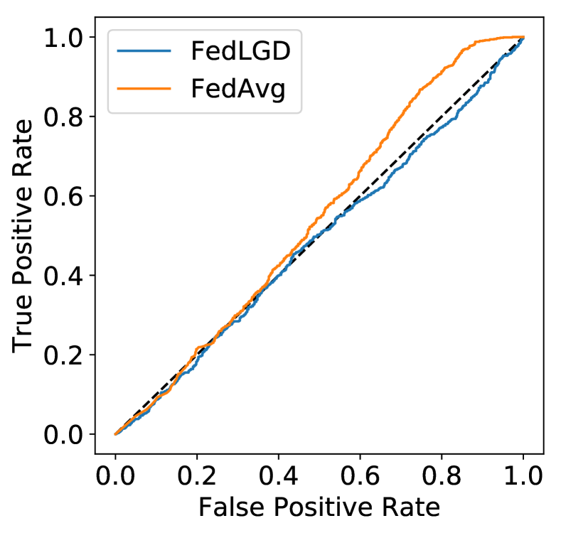
(a) MIA on Synth-Digits

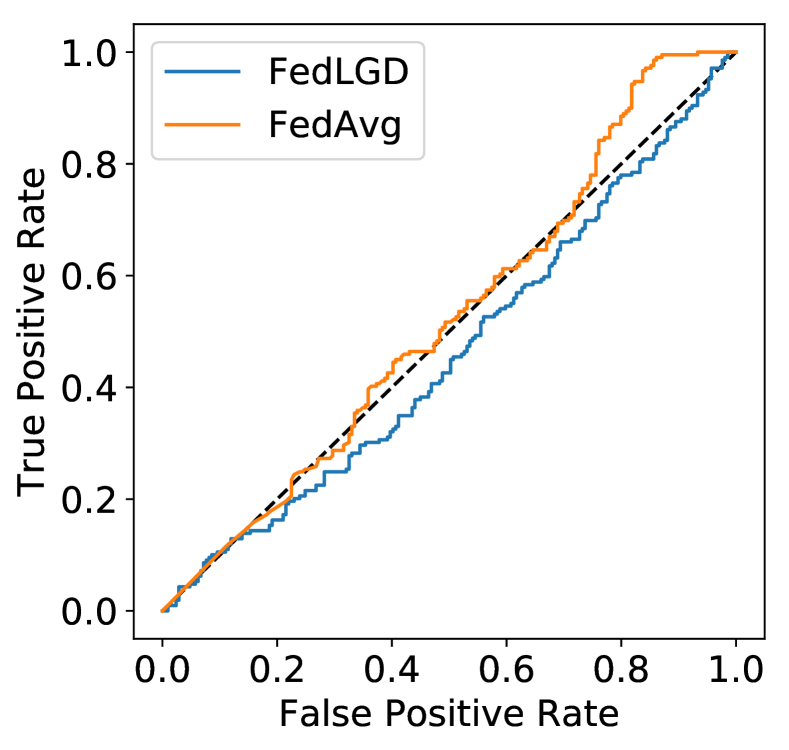
(b) MIA on MNIST-M

Figure 17: MIA attack results on models trained with FedAvg (using original dataset) and FedLGD (using distilled virtual dataset). If the ROC curve is the same as the diagonal line, it means the membership cannot be inferred. One can observe the ROC curve for the model trained with synthetic data is closer to the diagonal line, which indicates the membership information is harder to be inferred.

Appendix E Other Heterogeneous Federated Learning Methods Used in Comparison

FL trains the central model over a variety of distributed clients that contain non-iid data. We detailed each of the baseline methods we compared in Section 4 below.

FedAvg [29]

The most popular aggregation strategy in modern FL, Federated Averaging (FedAvg) [29], averages the uploaded clients’ model as the updated server model. Mathematically, the aggregation is represented as $w^{t+1}=w^{t}-\eta\sum_{i\in S_{t}}{\frac{|D_{i}|}{n}\Delta w_{k}^{t}}$ [23]. Because FedAVG is only capable of handling Non-IID data to a limited degree, current FL studies proposed improvements in either local training or global aggregation based on it.

FedProx [25]

FedProx improves local training by directly adding a $L_{2}$ regularization term, $\mu$, $\frac{\mu}{2}||w-w^{t}||^{2}$ controlled by hyperparameter $\mu$, in the local objection function to shorten the distance between the server and the client distance. Namely, this regularization enforces the updated model to be as close to the global optima as possible during aggregation. In our experiment, we carefully tuned $\mu$ to achieve the current results.

FedNova [38]

FedNova aims to tackle imbalances in the aggregation stage caused by different levels of training (e.g., a gap in local steps between different clients) before updating from different clients. The idea is to make larger local updates for clients with deep level of local training (e.g., a large local epoch). This way, FedNova scales and normalizes the clients’ model before sending them to the global model. Specifically, it improves its objective from FedAvg to $w^{t+1}=w^{t}-\eta\frac{\sum_{i\in S_{t}}{|D^{i}|\tau_{i}}}{n}\sum_{i\in S_{t}}{\frac{|D^{i}|\Delta w_{k}^{t}}{n\tau_{i}}}$ [23].

Scaffold [18]

Scaffold introduces variance reduction techniques to correct the ‘clients drift’ caused by gradient dissimilarity. Specifically, the variance on the server side is represented as $v$, and on the clients’ side is represented as $v_{i}$. The local control variant is then added as $v_{i}-v+\frac{1}{\tau_{i}\eta}(w^{t}-w_{i}^{t})$. At the same time, the Scaffold adds the drift on the client side as $w^{t}=w^{t}-\eta(\Delta(w_{t};b)-v_{i}^{t}+v)$ [23].

Virtual Homogeneous Learning (VHL) [37]

VHL proposes to calibrate local feature learning by adding a regularization term with global anchor for local training objectives $\mathbb{E}_{(x,y)\sim P_{k}}l(\rho\circ\psi(x),y)+\mathbb{E}_{(x,y)\sim P_{v}}l(\rho\circ\psi(x),y)+\lambda\mathbb{E}_{y}d(P_{k}(\psi(x)|y),P_{c}(\psi(x)|y))$. They theoretically and empirically show that adding the term can improve the FL performance. In the implementation, they use untrained StyleGAN [19] to generate global anchor data and leave it unchanged during training.

A comprehensive experimental study of FL can be found here [23]. Also, a survey of heterogeneous FL is here [48].

References

- [1] Abadi, M., Chu, A., Goodfellow, I., McMahan, H.B., Mironov, I., Talwar, K., Zhang, L.: Deep learning with differential privacy. In: Proceedings of the 2016 ACM SIGSAC conference on computer and communications security. pp. 308–318 (2016)
- [2] Batista, F.J.F., Diaz-Aleman, T., Sigut, J., Alayon, S., Arnay, R., Angel-Pereira, D.: Rim-one dl: A unified retinal image database for assessing glaucoma using deep learning. Image Analysis & Stereology 39(3), 161–167 (2020)
- [3] Carlini, N., Chien, S., Nasr, M., Song, S., Terzis, A., Tramer, F.: Membership inference attacks from first principles. In: 2022 IEEE Symposium on Security and Privacy (SP). pp. 1897–1914. IEEE (2022)
- [4] Carlini, N., Feldman, V., Nasr, M.: No free lunch in" privacy for free: How does dataset condensation help privacy". arXiv preprint arXiv:2209.14987 (2022)
- [5] Cazenavette, G., Wang, T., Torralba, A., Efros, A.A., Zhu, J.Y.: Dataset distillation by matching training trajectories. In: Proceedings of the IEEE/CVF Conference on Computer Vision and Pattern Recognition. pp. 4750–4759 (2022)
- [6] Diaz-Pinto, A., Morales, S., Naranjo, V., Köhler, T., Mossi, J.M., Navea, A.: Cnns for automatic glaucoma assessment using fundus images: an extensive validation. Biomedical engineering online 18(1), 1–19 (2019)
- [7] Dong, T., Zhao, B., Lyu, L.: Privacy for free: How does dataset condensation help privacy? arXiv preprint arXiv:2206.00240 (2022)
- [8] Franceschi, J.Y., De Bézenac, E., Ayed, I., Chen, M., Lamprier, S., Gallinari, P.: A neural tangent kernel perspective of gans. In: International Conference on Machine Learning. pp. 6660–6704. PMLR (2022)
- [9] Ganin, Y., Lempitsky, V.: Unsupervised domain adaptation by backpropagation. In: International conference on machine learning. pp. 1180–1189. PMLR (2015)
- [10] Goetz, J., Tewari, A.: Federated learning via synthetic data. arXiv preprint arXiv:2008.04489 (2020)
- [11] Gretton, A., Borgwardt, K.M., Rasch, M.J., Schölkopf, B., Smola, A.: A kernel two-sample test. The Journal of Machine Learning Research 13(1), 723–773 (2012)
- [12] Hard, A., Rao, K., Mathews, R., Ramaswamy, S., Beaufays, F., Augenstein, S., Eichner, H., Kiddon, C., Ramage, D.: Federated learning for mobile keyboard prediction. arXiv preprint arXiv:1811.03604 (2018)
- [13] He, K., Zhang, X., Ren, S., Sun, J.: Deep residual learning for image recognition. In: Proceedings of the IEEE conference on computer vision and pattern recognition. pp. 770–778 (2016)
- [14] Hendrycks, D., Dietterich, T.: Benchmarking neural network robustness to common corruptions and perturbations. arXiv preprint arXiv:1903.12261 (2019)
- [15] Hsu, T.M.H., Qi, H., Brown, M.: Measuring the effects of non-identical data distribution for federated visual classification. arXiv preprint arXiv:1909.06335 (2019)
- [16] Hu, S., Goetz, J., Malik, K., Zhan, H., Liu, Z., Liu, Y.: Fedsynth: Gradient compression via synthetic data in federated learning. arXiv preprint arXiv:2204.01273 (2022)
- [17] Hull, J.J.: A database for handwritten text recognition research. IEEE Transactions on pattern analysis and machine intelligence 16(5), 550–554 (1994)
- [18] Karimireddy, S.P., Kale, S., Mohri, M., Reddi, S., Stich, S., Suresh, A.T.: Scaffold: Stochastic controlled averaging for federated learning. In: International Conference on Machine Learning. pp. 5132–5143. PMLR (2020)
- [19] Karras, T., Laine, S., Aila, T.: A style-based generator architecture for generative adversarial networks. In: Proceedings of the IEEE/CVF conference on computer vision and pattern recognition. pp. 4401–4410 (2019)
- [20] Khosla, P., Teterwak, P., Wang, C., Sarna, A., Tian, Y., Isola, P., Maschinot, A., Liu, C., Krishnan, D.: Supervised contrastive learning. Advances in Neural Information Processing Systems 33, 18661–18673 (2020)
- [21] LeCun, Y., Bottou, L., Bengio, Y., Haffner, P.: Gradient-based learning applied to document recognition. Proceedings of the IEEE 86(11), 2278–2324 (1998)
- [22] Li, G., Togo, R., Ogawa, T., Haseyama, M.: Dataset distillation for medical dataset sharing. arXiv preprint arXiv:2209.14603 (2022)
- [23] Li, Q., Diao, Y., Chen, Q., He, B.: Federated learning on non-iid data silos: An experimental study. arXiv preprint arXiv:2102.02079 (2021)
- [24] Li, Q., He, B., Song, D.: Model-contrastive federated learning. In: Proceedings of the IEEE/CVF Conference on Computer Vision and Pattern Recognition. pp. 10713–10722 (2021)
- [25] Li, T., Sahu, A.K., Zaheer, M., Sanjabi, M., Talwalkar, A., Smith, V.: Federated optimization in heterogeneous networks. Proceedings of Machine Learning and Systems 2, 429–450 (2020)
- [26] Li, X., Huang, K., Yang, W., Wang, S., Zhang, Z.: On the convergence of fedavg on non-iid data. International Conference on Learning Representations (2020)
- [27] Lin, T., Kong, L., Stich, S.U., Jaggi, M.: Ensemble distillation for robust model fusion in federated learning. Advances in Neural Information Processing Systems 33, 2351–2363 (2020)
- [28] Van der Maaten, L., Hinton, G.: Visualizing data using t-sne. Journal of machine learning research 9(11) (2008)
- [29] McMahan, B., Moore, E., Ramage, D., Hampson, S., y Arcas, B.A.: Communication-efficient learning of deep networks from decentralized data. In: Artificial intelligence and statistics. pp. 1273–1282. PMLR (2017)
- [30] Mohamadi, M.A., Sutherland, D.J.: A fast, well-founded approximation to the empirical neural tangent kernel. arXiv preprint arXiv:2206.12543 (2022)
- [31] Netzer, Y., Wang, T., Coates, A., Bissacco, A., Wu, B., Ng, A.Y.: Reading digits in natural images with unsupervised feature learning (2011)
- [32] Orlando, J.I., Fu, H., Breda, J.B., van Keer, K., Bathula, D.R., Diaz-Pinto, A., Fang, R., Heng, P.A., Kim, J., Lee, J., et al.: Refuge challenge: A unified framework for evaluating automated methods for glaucoma assessment from fundus photographs. Medical image analysis 59, 101570 (2020)
- [33] Sachdeva, N., McAuley, J.: Data distillation: A survey. arXiv preprint arXiv:2301.04272 (2023)
- [34] Schuster, A.K., Erb, C., Hoffmann, E.M., Dietlein, T., Pfeiffer, N.: The diagnosis and treatment of glaucoma. Deutsches Ärzteblatt International 117(13), 225 (2020)
- [35] Shokri, R., Stronati, M., Song, C., Shmatikov, V.: Membership inference attacks against machine learning models. In: 2017 IEEE symposium on security and privacy (SP). pp. 3–18. IEEE (2017)
- [36] Sivaswamy, J., Krishnadas, S., Joshi, G.D., Jain, M., Tabish, A.U.S.: Drishti-gs: Retinal image dataset for optic nerve head (onh) segmentation. In: 2014 IEEE 11th international symposium on biomedical imaging (ISBI). pp. 53–56. IEEE (2014)
- [37] Tang, Z., Zhang, Y., Shi, S., He, X., Han, B., Chu, X.: Virtual homogeneity learning: Defending against data heterogeneity in federated learning. arXiv preprint arXiv:2206.02465 (2022)
- [38] Wang, J., Liu, Q., Liang, H., Joshi, G., Poor, H.V.: Tackling the objective inconsistency problem in heterogeneous federated optimization. Advances in neural information processing systems 33, 7611–7623 (2020)
- [39] Wang, T., Zhu, J.Y., Torralba, A., Efros, A.A.: Dataset distillation. arXiv preprint arXiv:1811.10959 (2018)
- [40] Xiong, Y., Wang, R., Cheng, M., Yu, F., Hsieh, C.J.: Feddm: Iterative distribution matching for communication-efficient federated learning. arXiv preprint arXiv:2207.09653 (2022)
- [41] Xu, J., Glicksberg, B.S., Su, C., Walker, P., Bian, J., Wang, F.: Federated learning for healthcare informatics. Journal of Healthcare Informatics Research 5, 1–19 (2021)
- [42] Ye, R., Ni, Z., Xu, C., Wang, J., Chen, S., Eldar, Y.C.: Fedfm: Anchor-based feature matching for data heterogeneity in federated learning. arXiv preprint arXiv:2210.07615 (2022)
- [43] Zhang, L., Shen, L., Ding, L., Tao, D., Duan, L.Y.: Fine-tuning global model via data-free knowledge distillation for non-iid federated learning. In: Proceedings of the IEEE/CVF Conference on Computer Vision and Pattern Recognition. pp. 10174–10183 (2022)
- [44] Zhao, B., Bilen, H.: Dataset condensation with differentiable siamese augmentation. In: International Conference on Machine Learning. pp. 12674–12685. PMLR (2021)
- [45] Zhao, B., Bilen, H.: Dataset condensation with distribution matching. In: Proceedings of the IEEE/CVF Winter Conference on Applications of Computer Vision. pp. 6514–6523 (2023)
- [46] Zhao, B., Mopuri, K.R., Bilen, H.: Dataset condensation with gradient matching. ICLR 1(2), 3 (2021)
- [47] Zhou, T., Zhang, J., Tsang, D.: Fedfa: Federated learning with feature anchors to align feature and classifier for heterogeneous data. arXiv preprint arXiv:2211.09299 (2022)
- [48] Zhu, H., Xu, J., Liu, S., Jin, Y.: Federated learning on non-iid data: A survey. Neurocomputing 465, 371–390 (2021)
- [49] Zhu, L., Liu, Z., Han, S.: Deep leakage from gradients. Advances in neural information processing systems 32 (2019)