Nature of spinons in the 1D spin chains

Abstract

We provide an intuitive understanding of the collective low-energy spin excitation of the one-dimensional spin-$\frac{1}{2}$ antiferromagnetic Heisenberg chain, known as the spinon. To this end, we demonstrate how a single spinon can be excited by adding one extra spin to the ground state. This procedure accurately reproduces all key features of the spinon’s dispersion. These follow from the vanishing norm of the excited state which is triggered by the ground state entanglement. Next, we show that the spinon dispersion can be approximately reproduced if we replace the true ground state with the simplest valence-bond solid. This proves that the spinon of the one-dimensional Heisenberg model can be understood as a single spin flowing through a valence-bond solid.

Introduction: Some of the most amenable states of interacting quantum matter are those with long-range order Khomskii (2010), due to their almost classical, product-like, ground states. Their low-lying excited states are also rather simple, being best described in terms of long-living and weakly interacting collective excitations Khomskii (2010); Venema et al. (2016) whose nature is extremely intuitive. For instance, a magnon in a ferromagnet (FM) Auerbach (1994) propagates just like a free particle, see Fig. 1(a).

However, even relatively small deviations from a ground state with long-range order may lead to surprisingly complex excited states. Probably the best known and most studied such example is the one-dimensional (1D) spin-$\frac{1}{2}$ antiferromagnetic (AF) Heisenberg model Bethe (1931); Auerbach (1994). Its ground state has quasi-long-range order, with correlations that decay algebraically with distance Auerbach (1994). Its low-lying excited states are interpreted in terms of spinons, which are rather exotic quasiparticles with a peculiar dispersion that is supported only in half of the Brillouin zone and with a bandwidth proportional to $\pi$ Faddeev and Takhtajan (1981), and have so far evaded an intuitive picture.

The complex nature of the spinon is confirmed by the slow historical development of its understanding: while the Bethe Ansatz solution for the Heisenberg model has been known for over 90 years Bethe (1931), it was realised only after 50 years that the spinon carries spin-$\frac{1}{2}$ Faddeev and Takhtajan (1981) instead of the previously assumed spin-$1$ des Cloizeaux and Pearson (1962) of a magnon-like excitation. One reason why understanding the spinon’s properties was so difficult is that standard experimental probes do not excite a single spinon. Instead they excite spin-$1$ flips which decay into the two-spinon (and higher-order) continua Tennant et al. (1993); Lake et al. (2005); Caux and Maillet (2005); Klauser et al. (2011); Schlappa et al. (2012); Mourigal et al. (2013); Ferrari et al. (2018). This process is usually visualised as the creation of two freely moving domain walls propagating in a Néel AF, cf. Fig. 1(b). As we show here, this simple cartoon is not a valid picture of the spinon.

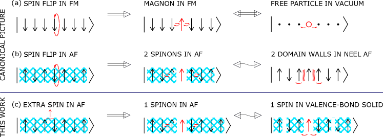
Figure 1: Cartoon views of collective excitations in spin-$\frac{1}{2}$ Heisenberg chains. Panel (a): canonical picture arising after flipping one spin in the Heisenberg FM ground state (left subpanel) and triggering a propagating magnon (middle subpanel) which is understood as a free mobile particle in the vacuum (right subpanel). Panel (b): canonical picture arising after flipping one spin in the Heisenberg AF ground state (left subpanel) and triggering two propagating spinons (middle subpanel) which are usually approximately understood as two mobile domain walls in a Néel AF (right subpanel). Panel (c): picture introduced in this paper, arising after inserting an additional spin in the Heisenberg AF ground state (left subpanel) and triggering a propagating spinon (middle subpanel) which can be understood as a mobile spin flowing in the valence-bond solid (right subpanel). Flipped or inserted spins are shown in red; entanglement between two or more sites is shown by a blue-coloured hatched area.

In this Letter, we provide a new and intuitive understanding of the spinon’s nature. To this end, we first propose a procedure to create a state with a single spinon excitation by adding one extra spin site to the ground state of a Heisenberg spin chain, cf. Fig. 1(c). Indeed, we show that this accurately reproduces all key features of the spinon’s dispersion and this excitation carries spin-$\frac{1}{2}$ by construction. While our procedure is closely related to the concepts promoted in Refs. Sorella and Parola (1992); Talstra and Strong (1997); Penc et al. (1997); Penc and Serhan (1997); Matveev et al. (2007a, b), it has an advantage of being simple and and easily amenable to numerical implementation.

We then move to the main results of this Letter. We first demonstrate that a domain wall propagating through a Néel state is qualitatively different from a spinon, invalidating the popular naive picture of Fig. 1(b). Remarkably, we find a good approximation of the spinon if we replace the true AF ground state with the simplest valence-bond solid. This result is due to entanglement, which is a characteristic feature both of the Heisenberg spin chain ground state Vidal et al. (2003a); Sato et al. (2006); Miwa and Smirnov (2019); Murciano et al. (2020); Niezgoda et al. (2020) and of the valence-bond solid Alet et al. (2007) and which is absent in the Néel state. Altogether, this enables us to draw the following intuitive explanation of the key spinon properties: (i) the limited support of the spinon dispersion stems from entangled fluctuating spins leading to destructive interference of the spinon wave for $|q|>\pi/2$; (ii) the low-energy linear dispersion arises both because of (i) and because a single spin can hop between adjacent sites in the valence-bond state, cf. Fig. 1(c).

The model: The Hamiltonian of the Heisenberg spin chain is Bethe (1931); Korepin et al. (1993)

$$H_{L}=J\sum_{j=1}^{L}\vec{\sigma}_{j}\cdot\vec{\sigma}_{j+1},$$ (1)

where $\vec{\sigma}_{j}=(\sigma_{j}^{x},\sigma_{j}^{y},\sigma_{j}^{z})$ are spin-$\frac{1}{2}$ Pauli matrices acting on the $j$-th site of the chain. We assume periodic boundary conditions, $\vec{\sigma}_{L+1}=\vec{\sigma}_{1}$. In the antiferromagnetic case $J>0$ and in the following we set $J=1$.

The 1D Heisenberg model is exactly solvable with the Bethe Ansatz Korepin et al. (1993). For the AF case and even $L$, it has a unique ground state and its magnetization $M=\sum_{j=1}^{L}\sigma_{j}^{z}$ is zero. For odd $L$, the ground state is doubly degenerate. The low-energy excitations above the ground state are obtained by exciting an even number of spinons. A single spinon has spin-$\frac{1}{2}$ and its dispersion relation

$$\varepsilon(q)=\frac{\pi}{2}\cos q,\quad q\in\bigg{[}-\frac{\pi}{2},\frac{\pi}{2}\bigg{]}$$ (2)

is supported only in half of the Brillouin zone Faddeev and Takhtajan (1981). While the Bethe Ansatz provides an exact description of the spinon, it lacks a physically intuitive picture.

How to create a single spinon: We now present a general method of constructing elementary excitations for any spin chain. As we show next, when applied to the Heisenberg chain, its result is a single spinon excitation.

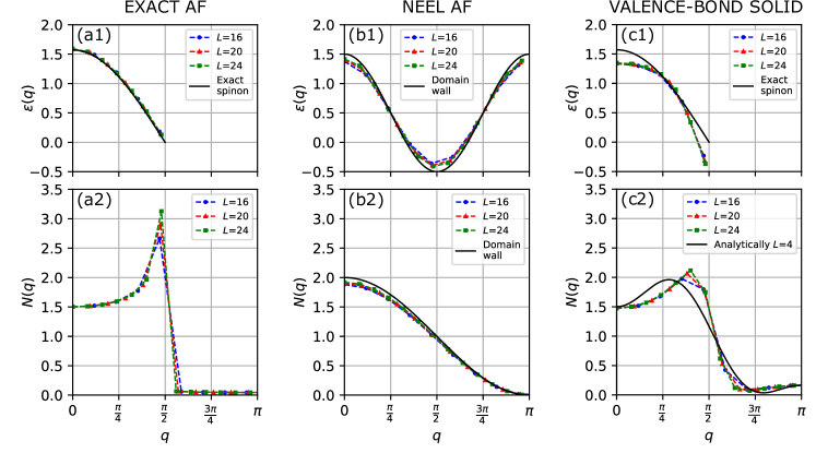
Figure 2: Top panels show the dispersion $\varepsilon(q)$ of the excitation, defined in Eq. (7), while the bottom panels show the norm $N(q)=\langle\psi(q)|\psi(q)\rangle$. The excited state $|\psi(q)\rangle$ of Eq. (6) is built: from the exact AF ground state $|\Psi_{0}\rangle$ obtained by numerically diagonalising the Heisenberg Hamiltonian on $L$ sites [panels (a1)-(a2)]; by using the Néel AF state of Eq. (9) instead of $|\Psi_{0}\rangle$ [panels (b1)-(b2)]; by using the spin valence-bond solid state of Eq. (10) instead of $|\Psi_{0}\rangle$ [panels (c1)-(c2)]. Results for chains of various length $L$ are shown by symbols (the connecting dashed lines are guides to the eye). The thick black solid lines show the relevant analytical expressions, for comparison purposes (see text for more details).

For the spin chain of length $L$, we assume that we know the expansion of its ground state in the local spin basis:

$$|\Psi_{0}\rangle=\sum_{j}A_{j}|j\rangle.$$ (3)

In principle $j$ extends over $2^{L}$ possible local states, however in practice various selection rules force many $A_{j}$ to vanish. For example, for $L$ even and if $|\Psi_{0}\rangle$ has total magnetization $M=0$, the sum includes maximally $\binom{L}{L/2}\sim\frac{2^{L}}{\sqrt{L}}$ states. The coefficients $A_{j}$ can be obtained from exact diagonalization or, for integrable spin chains, by the coordinate Bethe Ansatz Korepin et al. (1993).

Next, we insert a new site with a spin up between sites $m-1$ and $m$ of the original chain, thus extending the chain length to $L+1$ sites, cf. left panel of Fig. 1(c). Specifically, for each state $|j\rangle$ expressed in the local spin basis this creates a uniquely defined state $|j(m)\rangle$, $m=0,\dots,L$,

$$|j\rangle=|\!\underbrace{\downarrow\downarrow\cdots\uparrow}_{L}\rangle\;\rightarrow\;|j(m)\rangle=|\!\underbrace{\downarrow\downarrow\cdots}_{m-1}\uparrow\!\!\!\underbrace{\cdots\uparrow}_{L-m+1}\!\!\rangle.$$ (4)

The resulting basis $|j(m)\rangle$ is over-complete because it contains $2^{L}(L+1)$ states. We use it to define an approximate excited state

$$|\Psi(m)\rangle=\sum_{j}A_{j}|j(m)\rangle.$$ (5)

An important feature of the construction, further discussed below, is that $|\Psi(m)\rangle$ is not normalized. Denoting by $|\bar{\Psi}(m)\rangle$ its normalized counterpart, we find the first two moments of the local spin operators to be $\langle\bar{\Psi}(m)|\sigma_{j}^{z}|\bar{\Psi}(m)\rangle=\frac{\delta_{jm}}{2}$, $\langle\bar{\Psi}(m)|(\sigma_{m}^{z})^{2}|\bar{\Psi}(m)\rangle=\frac{1}{4}$, and for $j\neq m$: $\langle\bar{\Psi}(m)|(\sigma_{j}^{z})^{2}|\bar{\Psi}(m)\rangle=\langle\Psi_{0}|(\sigma_{1}^{z})^{2}|\Psi_{0}\rangle$, where in the last equality we used the translational invariance of the ground state. This result can be visualized as a spin up frozen at the $m^{th}$ site of the $L+1$-site chain, in the sea of fluctuating spins on all other sites. These fluctuations are identical to the ground state fluctuations of the $L$-site chain, by construction. This picture is in accordance with the concept of elementary excitations which are created from the ground state, and inherit rather than rebuild the correlations present in it.

To define a dispersion relation we introduce a Fourier transform with momentum $q=\frac{2\pi n}{L+1}$, $-L/2\leqslant n\leqslant L/2$, $n\in\mathbb{Z}$:

$$|\Psi(q)\rangle=\frac{1}{\sqrt{L+1}}\sum^{L}_{m=0}e^{iqm}|\Psi(m)\rangle.$$ (6)

The state $|\Psi(q)\rangle$ is not an eigenstate of the Hamiltonian, so we define its energy as the expectation value and calculate it with respect to the ground state energy $E_{0}^{L+1}$ of a system of size $L+1$:

$$\varepsilon(q)=\frac{\langle\Psi(q)|H_{L+1}|\Psi(q)\rangle}{\langle\Psi(q)|\Psi(q)\rangle}-E^{L+1}_{0},$$ (7)

where $H_{L+1}$ is the Hamiltonian for a system of size $L+1$.

Spinon in the AF Heisenberg chain: We now show that if we apply the procedure outlined above to the Heisenberg spin-$\frac{1}{2}$ chain, we recover the spinon dispersion relation (2) including the correct support of half of the Brillouin zone. The amplitudes $A_{j}$ are computed from exact diagonalization. The results are shown in Fig. 2(a1). We observe that the spinon dispersion relation $\varepsilon(q)$, shown by the black solid line, is recovered with excellent precision. To understand this result, we also plot separately the denominator of Eq. (7), namely:

$$N(q)=\langle\Psi(q)|\Psi(q)\rangle.$$ (8)

We find that $N(q)$ vanishes (similarly to Talstra and Strong (1997), its value is negligible) for $|q|>\pi/2$, cf. Fig. 2(a2). States of zero norm are not physical and therefore we exclude them from further considerations. The consequence is that the spinon only exists in half of the Brillouin zone.

In our procedure, the correlations present in the spinon state are inherited from the ground state. This leads to the natural question as to which correlations, of all those present in the exact ground state, are most relevant to the spinon. To answer this question we consider two approximations to the ground state: (i) the lowest energy classical configuration, i.e. the Néel state, and (ii) the simplest valence-bond solid.

(i) Domain wall approximation: In the first approximation, we therefore replace:

$$|\Psi_{0}\rangle\approx|\!\uparrow\downarrow\uparrow\downarrow\uparrow\downarrow\uparrow\downarrow\ldots\rangle.$$ (9)

We then apply the procedure to this wavefunction, see left subpanel of Fig. 1. The results for the corresponding $\varepsilon(q)$ and $N(q)$ are shown in Fig. 2(b1-b2).

This dispersion $\varepsilon(q)$ reproduces the domain wall dispersion found in the Ising-like AF Villain (1975), $\varepsilon_{dw}(q)=\frac{1}{2}+\cos(2q)$, shown as a solid black line in Fig. 2(b1), instead of the spinon dispersion. This difference is directly caused by the use of the Néel state instead of the true ground state in the procedure.

(ii) Additional spin in valence-bond solid: As a second approximation, we replace the ground state with a valence-bond solid:

$$|\Psi_{0}\rangle\approx\frac{|\!\uparrow\downarrow\rangle-|\!\downarrow\uparrow\rangle}{\sqrt{2}}\otimes\frac{|\!\uparrow\downarrow\rangle-|\!\downarrow\uparrow\rangle}{\sqrt{2}}\otimes\ldots,$$ (10)

leading to a spin being added (in our procedure) to a state consisting of singlets on neighbouring sites, cf. right subpanel of  Fig 1(c).

The corresponding $\varepsilon(q)$, $N(q)$ are shown in Fig. 2(c1-c2). The dispersion relation is qualitatively similar to the spinon dispersion (black solid line). Quantitatively, the value at $q=0$ is underestimated and the value at $q=\frac{\pi}{2}$ is negative, reflecting the fact that the valence-bond state is an approximation. Indeed, its average energy per site is $-0.3750$, significantly larger than the exact ground state energy per site of $-0.4438$ Auerbach (1994).

We emphasize that this approximation recovers the linear low-energy dispersion $\varepsilon(q)\propto|{\pi\over 2}-q|$ as $q\rightarrow{\pi\over 2}$ and the extended region $|q|\gtrsim\pi/2$ where the norm $N(q)$ nearly vanishes. The latter is similar to the result of exact diagonalization presented in Fig. 2(a2). Interestingly, it is qualitatively the same as an exact result for a short $L=4$ chain, see Fig. 2(c2) and Sec. I of SM , which further supports the close connection between the valence-bond approximation and the exact result.

Contrasting the two approximations reveals the crucial role played by a particular form of the ground state correlations – that is quantum entanglement – in determining the spinon properties. We further discuss the two main characteristics below.

The limited support of the spinon dispersion: By excluding from the Hilbert space states of zero norm, the question of the support of the spinon dispersion is translated into the question of a (nearly) vanishing $N(q)$. To understand the key role played by the ground state entanglement, let us consider the structure of $|\Psi(q)\rangle=\sum_{j^{\prime}}B_{j^{\prime}}(q)|j^{\prime}\rangle$ expressed in the spin basis of the longer chain. Any new spin configuration $|j^{\prime}\rangle$ is obtained from all of the original states of the shorter chain $|j\rangle$ that differ from $|j^{\prime}\rangle$ only through a missing spin up. Insertion of the missing spin up will generate $|j^{\prime}\rangle$, however because these inserted spins up are at different positions, different contributions are multiplied by different Fourier factors $e^{iqm}$ in $B_{j^{\prime}}(q)$.

Crucially, a configuration $|j^{\prime}\rangle$ may originate from multiple $|j\rangle$’s in multiple ways. This gives rise to the momentum dependence of the norm $N(q)$, even for a product ground state. For example, consider a Néel ground state, i.e. a unique $|j\rangle=|\!\!\uparrow\downarrow\uparrow\downarrow\dots\rangle$, and let $|j^{\prime}\rangle=|\!\!\uparrow\uparrow\downarrow\uparrow\downarrow\dots\rangle$. This state can be obtained from $|j\rangle$ by inserting the extra spin up either before or after the first spin up already present. The Fourier coefficients of these two contributions differ by $e^{iq}$, $B_{j^{\prime}}(q)=1+e^{iq}$, therefore for the Néel state the norm vanishes at $q=\pi$, as seen in Fig. 2(b2).

In an entangled ground state, however, a $|j^{\prime}\rangle$ can be reached by adding a spin in different places in different $|j\rangle$ configurations. To illustrate this, consider the $L=4$-site Heisenberg chain, see Sec. I of SM for details. Its ground state is entangled and includes, inter alia, the two contributions: (i) $|\uparrow\downarrow\uparrow\downarrow\rangle$, and (ii) $-\frac{1}{2}|\uparrow\uparrow\downarrow\downarrow\rangle$. If we add a spin up, before or after the first spin, in (i) and after the third spin in (ii), respectively, we reach the same $|j^{\prime}\rangle=|\!\!\uparrow\uparrow\downarrow\uparrow\downarrow\rangle$ with different phase factors, leading to $B_{j^{\prime}}(q)=1+e^{iq}-e^{3iq}/2$.

It is crucial in the above-obtained equation that the different factors have different phases. On one hand, it leads to the nearly vanishing norm $N(q)$ in an extensive region of momenta $q$, see Sec. I of [SM] for more details. On the other hand, such a non-trivial relative phase factor in front of the Fourier coefficient $e^{imq}$ can only be obtained for the ground state that is entangled. Physically this means that the ‘fluctuating’ spins stemming from the entangled ground state, lead to a (nearly) destructive interference in the spinon wave and thus to the (nearly) vanishing of its norm $N(q)$ for some momenta. Last but not least, we put this qualitative analysis on firm ground by proving that $N(0)$ is an entanglement witness: As shown in Sec. II of SM , for a translationally invariant superposition of product states of zero magnetization $N(0)\geq 2$. Therefore, $N(0)<2$ signals an entangled ground state.

However, there is more to the norm $N(q)$ than that, as it can behave as a function of $q$ in rather extreme ways: it may vanish for an extensive range of momenta $q$, or may diverge. This happens for the exact ground state of the Heisenberg model in the thermodynamic limit, though not for the finite Heisenberg chains or the valence-bond solid [cf. panels (a) and (c) of Fig. 2]. This observation is in agreement with the notion of the short-range entanglement present in the ground state of the Heisenberg model in the thermodynamic limit Vidal et al. (2003b) and the semi-local (‘minimal’) entanglement of the valence-bond ground state Alet et al. (2007). This shows that $N(q)$ contains rich information about the structure of the state and further studies are required to fully harvest its potential.

Dispersion linear in momentum: The other notable feature of the spinon dispersion is its linear dependence on $q$ in the low-energy limit. It can be understood as a result of (i) the vanishing compact support for $|q|>\pi/2$ that is due to ground state entanglement (see above), and (ii) the $\propto\cos q$ dispersion relation arising from nearest neighbor hopping of the spinon, discussed next.

To this end we note that the linear dispersion relation is (is not) reproduced when the single spin is added to the valence-bond (Néel) state, cf. Fig. 2(b-c). This is because in the valence-bond state the singlets ‘resonate’ with each other as well as with the added spin and move by one site with a single action of the Hamiltonian. On the other hand, a domain wall in the Neel state can only move between next nearest neighbour sites.

Outlook: The postulated procedure is universal and can be applied to any 1D spin model, cf. Sec. III of SM for a short overview. In particular, it can be used to study excitations of the 1D FM chain, see Fig. 2(a-b) of SM : in this case a single magnon is excited in the procedure. This further shows that the spinon is not exotic because it can be excited in quite a special manner but it is the entanglement nature of the antiferromagnetic ground state that is crucial here. We suggest that in the future, this procedure can be used to explore the nature of the elementary excitations in frustrated spin systems, such as the recently discussed problem of marginally irrelevant interactions between spinons in $J_{1}-J_{2}$ spin chains Keselman et al. (2020). We propose to generalise the procedure to higher dimensions by focusing on the Green’s function of an immobile hole added to a spin system, for this corresponds to removing a spin from a lattice.

Conclusions: Our work confirms a paradigm that is rarely explicitly formulated, according to which a collective excitation generally inherits its properties from the ground state. This paradigm is probably best exemplified by the Goldstone theorem and the close relation between the broken-symmetry long-range ordered ground state and the gapless collective excitations Beekman et al. (2019).

Here we used this paradigm to understand a system that does not have spontaneous symmetry breaking and where the Goldstone theorem is not valid, hence the connection between the ground and the excited states is less clear. Our successful explanation of the properties of the spinon excitation shows that such a connection is possible in complex correlated systems as well. The resulting features of the elementary excitations are then controlled by the entanglement in the ground state.

SUPPLEMENTAL MATERIAL

I Exact result for the $4$-site Heisenberg chain: relation between the norm $N(q)$ and entanglement

We discuss below the AF Heisenberg chain on $L=4$ sites. Here the resonating valence-bond state is an exact ground state of the Heisenberg model. Up to normalization,

$$|\Psi_{0}\rangle=\frac{|\!\uparrow\downarrow\rangle-|\!\downarrow\uparrow\rangle}{\sqrt{2}}\otimes\frac{|\!\uparrow\downarrow\rangle-|\!\downarrow\uparrow\rangle}{\sqrt{2}}+{\rm(translation)}.$$ (11)

By following our procedure, we find:

$$|\Psi(q)\rangle=\frac{1+e^{iq}-\frac{e^{3iq}}{2}}{\sqrt{3}}|A\rangle-\frac{1+e^{iq}+e^{2iq}}{2\sqrt{3}}|B\rangle$$ (12)

with $|A\rangle\!\!\!=\!\!\!|\!\!\uparrow\uparrow\downarrow\uparrow\downarrow\rangle\!\!+\!\!({\rm translations})$, $|B\rangle\!\!\!=\!|\!\!\uparrow\uparrow\uparrow\downarrow\downarrow\rangle+({\rm translations})$. All the states in $|A\rangle$ and $|B\rangle$ are orthonormal to each other. The resulting norm:

$$N(q)=1+\cos q-\frac{1}{6}\cos(2q)-\frac{1}{3}\cos(3q)$$ (13)

shows, inter alia, a considerable suppression of $N(q)$ in an extended interval from around $\frac{\pi}{2}$ to $\pi$, see black solid line in Fig. 2(c2) of the main text and discussion below. Of course, for $L=4$ this result is only meaningful at multiples of $q=\frac{2\pi}{5}$, but similar arguments hold for longer chains within the valence-bond approximation.

Having obtained an exact expression for $N(q)$, (13), we are now ready to investigate the origin of its two main striking properties: (i) a relative enhancement of the $4$-site Heisenberg chain norm, with a pronounced maximum for the small momenta $q\lesssim\pi/2$, w.r.t. the norm obtained once a spin is added to the Neel antiferromagnet, that is w.r.t. $N(q)=1+\cos(q)$ (see main text); (ii) a relative suppression of the $4$-site Heisenberg chain norm, with a pronounced minimum for the small momenta $q\gtrsim\pi/2$, w.r.t. the norm obtained once a spin is added to the Neel antiferromagnet, that is w.r.t. $N(q)=1+\cos(q)$ (see main text).

To this end, let us first note that a sum rule $\sum_{0<q<\pi}N(q)=\pi$ means that once we e.g. understand the relative enhancement for some momenta, then the relative suppression for the other momenta follows. Therefore, we concentrate on investigating the former effect.

A quick inspection of Eq. (13) shows that the term responsible for obtaining such a relative enhancement in $N(q)$ for small momenta (and, conversely, also a relative suppression for large momenta) is the term $\propto-\cos(3q)$. A closer look at the procedure of adding an extra spin shows that, in order to obtain such a contribution to the norm, there must exist two product states in the ground state which contribute to $|\Psi_{0}\rangle$ with opposite sign and that they must be identical to each other after adding an extra spin in our procedure, modulo a phase factor $e^{3iq}$. This is fulfilled for instance by such two contributions to the exact ground state $|\Psi_{0}\rangle$ that, upon adding an extra spin site at particular location, lead to the same states which differ by $e^{3iq}$ in our procedure:

$$|\uparrow\downarrow\uparrow\downarrow\rangle\quad \rightarrow\quad|\tilde{\uparrow}\uparrow\downarrow\uparrow\downarrow\rangle,$$ (14)

$$-\frac{1}{2}|\uparrow\uparrow\downarrow\downarrow\rangle\quad \rightarrow\quad-\frac{1}{2}e^{3iq}|\uparrow\uparrow\downarrow\tilde{\uparrow}\downarrow\rangle,$$ (15)

where the tilde sign denotes the added spin. Note that when the spin up is added after the first spin in $|\uparrow\downarrow\uparrow\downarrow\rangle$, then we obtain the same configuration $|\uparrow\uparrow\downarrow{\uparrow}\downarrow\rangle$—albeit with a factor of $e^{iq}$.

Identifying the type of product states in $|\Psi_{0}\rangle$ that lead to the relative enhancement of the norm $N(q)$ for small momenta, allows us to intuitively understand the origin of this phenomenon: namely, it follows from the valence bond nature of the ground state—the two ‘fluctuating singlets’ allow for the onset of ferromagnetic domains with opposite magnetisation and a (relative) negative phase contribution to the ground state, see Eq. (15). Note that the relative negative phase is just as crucial as the existence of ferromagnetic domains and that such a phase difference can only be realised once $|\Psi_{0}\rangle$ is not a product state. Altogether, this shows how specific properties of the norm $N(q)$ of the state constructed by adding one extra spin can be related to the entangled nature of the spin chain ground state $|\Psi_{0}\rangle$.

II The norm $N(0)$ as an entanglement witness

In this section we demonstrate a relation between $N(0)$ and the entanglement present in the ground state $|\Psi\rangle$. More specifically, we derive an exact lower bound $N(0)\geq 2$ for product states. This result further promotes $N(q)$ to be a quantity providing useful information about the system and not merely a normalization. To this end, we reformulate the construction of the excited states by introducing operatorial formalism.

We start by introducing operators $c_{j}$ that add a site between sites $j-1$ and $j$ and occupy it with a spin up. They act as the identity on the remaining lattice sites. Similar operators were considered before in the context of lattice supersymmetry Hagendorf and Liénardy (2017). Using the notation introduced in the main text,

$$|\Psi(m)\rangle=c_{m}|\Psi_{0}\rangle.$$ (16)

From the local operators $c_{j}$ we built operators $C_{L}$ and $\bar{C}_{L}$ which act on the whole chain

$$C_{L}=\sum_{j=0}^{L-1}c_{j},\qquad\bar{C}_{L}=\sum_{j=0}^{L}c_{j}.$$ (17)

The result of their action on a single state is a superposition of states with an extra spin-up inserted before each lattice site (for $C_{L}$) and additionally also after the last site (for $\bar{C}_{L}$). With this formalism the excited state at $q=0$ can be written as

$$|\Psi(q=0)\rangle=\frac{1}{\sqrt{L+1}}\bar{C}_{L}|\Psi_{0}\rangle.$$ (18)

and

$$N(0)=\frac{1}{L+1}\frac{\langle\Psi_{0}|\bar{C}_{L}^{\dagger}\bar{C}_{L}|\Psi_{0}\rangle}{\langle\Psi_{0}|\Psi_{0}\rangle},$$ (19)

where we explicitly included the norm.

In the main text we consider systems with periodic boundary conditions. Their ground states are translationally invariant which has important consequences for the evaluation of $N(0)$. Any translationally invariant state can be generated from a seed state by considering a superposition of all its translations. To formalize this, let us define operator $t_{n}$ translating a state by $n$ sites to the right and respecting the periodic boundary condition. Similarly, we define $T_{L}=\sum_{n=0}^{L-1}t_{n}$. For any translationally invariant state $|\Psi_{0}\rangle$ there exists a state $|\Psi\rangle$ such that $|\Psi_{0}\rangle=T_{L}|\Psi\rangle$ where $|\Psi\rangle$ plays a role of a seed state. Note that if two states $|\Psi_{1}\rangle$ and $|\Psi_{2}\rangle$ are related by a translation, i.e. there exist $m=1,\dots L-1$ such that $t_{m}|\Psi_{1}\rangle=|\Psi_{2}\rangle$ then $T_{L}|\Psi_{1}\rangle=T_{L}|\Psi_{2}\rangle$. This implies that a translationally invariant state can be generated from any of its seed states.

Being seed states of the same state $|\Psi_{0}\rangle$ is an equivalence relation and therefore any translationally invariant state can be associated with an equivalence class of its seed states that we denote $[|\Psi_{0}\rangle]$ and which is characterized by the following defining property

$$T_{L}|\Psi_{1}\rangle=T_{L}|\Psi_{2}\rangle,\qquad|\Psi_{i}\rangle\in[|\Psi_{0}\rangle].$$ (20)

We will use now this notion to reformulate the computation of $N(0)$ for a translationally invariant states. To avoid confusions we denote by $\mathcal{N}$ the value of $N(0)$ for translationally invariant state.

As discussed above, for a translationally invariant state $|\Psi_{0}\rangle$ there exist $|\Psi\rangle$ such that $|\Psi_{0}\rangle=T|\Psi\rangle$. Therefore

$$\mathcal{N}_{\Psi_{0}}=\frac{1}{L+1}\frac{\langle\Psi|T_{L}^{\dagger}\bar{C}_{L}^{\dagger}\bar{C}_{L}T_{L}|\Psi\rangle}{\langle\Psi|T_{L}^{\dagger}T_{L}|\Psi\rangle}.$$ (21)

From the property (20) it follows that $\mathcal{N}$ is the same for any $|\Psi\rangle$ in the equivalance class $[|\Psi_{0}\rangle]$ of $|\Psi_{0}\rangle$. This implies that to compute $\mathcal{N}$ for a translationally invariant state we can identify one of its seeds and then use equation (21). This equation still explicitly symmetrizes over all translations but we will now rewrite in a form more suitable for further computations. In this process the above mentioned symmetry becomes less obvious.

We start by describing some properties of operators $C_{L}$, $\bar{C_{L}}$ and $T_{L}$. First we observe that $T_{L}$ is hermitian and has a simple property $T_{L}^{2}=LT_{L}$. Furthermore the following relations $\bar{C}_{L}T_{L}=T_{L+1}C_{L}$ and $\bar{C}_{L}T_{L}=T_{L+1}c_{m}T_{L}$, with $m=0,\dots,L$, hold. Specifically, the first relation shows why in our procedure we insert the extra spin before and after the chain. This is because when this operation is applied to a translationally invariant state it produces a translationally invariant state.

Using the properties of operators $C_{L}$ and $T_{L}$ we can prove a simple property of $\langle\Psi_{0}|\bar{C}_{L}^{\dagger}\bar{C}_{L}|\Psi_{0}\rangle$ that, due to the translational invariance, position of one of the insertions can be fixed,

$$\langle\Psi_{0}|\bar{C}_{L}^{\dagger}\bar{C}_{L}|\Psi_{0}\rangle =\langle\Psi|T_{L}\bar{C}_{L}^{\dagger}\bar{C}_{L}T_{L}|\Psi\rangle$$

$$=\langle\Psi|C_{L}^{\dagger}T_{L+1}T_{L+1}c_{m}T_{L}|\Psi\rangle$$

$$=(L+1)\langle\Psi|\bar{C}_{L}^{\dagger}T_{L+1}c_{m}T_{L}|\Psi\rangle.$$ (22)

This leads to an equivalent expression for $\mathcal{N}$

$$\mathcal{N}=\frac{1}{L}\frac{\langle\Psi|T_{L}\bar{C}_{L}^{\dagger}c_{0}T_{L}|\Psi\rangle}{\langle\Psi|T_{L}|\Psi\rangle}.$$ (23)

We will now use this representation to prove a bound on $\mathcal{N}$ if $|\Psi\rangle$ is a product state and has an inner symmetry under translations. To this end we introduce a notion of states partially invariant under translations. That is for such state $|\Psi\rangle$ there exists a minimal non-zero $m$ such that

$$t_{m}|\Psi\rangle=|\Psi\rangle.$$ (24)

We observe that the property of the partial invariance is shared by all the states in the same equivalance class. The consequence of this is that if additionally $|\Psi\rangle$ is a product state then it can be written as a tensor product of its elementary cells

$$|\Psi\rangle=\bigotimes_{i=1}^{k}|\psi\rangle,$$ (25)

with $L=mk$.

Bound for partially invariant product states: We will now show that

$$\mathcal{N}_{\Psi_{0}}\geq N_{\psi_{0}}.$$ (26)

Assuming (24) we have $T_{L}|\Psi\rangle=kT_{m}|\Psi\rangle$. We then find

$$\mathcal{N}_{\Psi_{0}} =\frac{1}{L}\frac{\langle\Psi|T_{L}\bar{C}_{L}^{\dagger}c_{0}T_{L}|\Psi\rangle}{\langle\Psi|T_{L}|\Psi\rangle}=\frac{1}{m}\frac{\langle\Psi|T_{m}\bar{C}_{L}^{\dagger}c_{0}T_{m}|\Psi\rangle}{\langle\Psi|\Psi\rangle}$$

$$\geq\frac{1}{m}\frac{\langle\Psi|T_{m}\bar{C}_{m}^{\dagger}c_{0}T_{m}|\Psi\rangle}{\langle\Psi|\Psi\rangle}=\frac{1}{m}\frac{\langle\psi|T_{m}\bar{C}_{m}^{\dagger}c_{0}T_{m}|\psi\rangle}{\langle\psi|\psi\rangle}=\mathcal{N}_{\psi_{0}},$$ (27)

where the inequality is a consequence of truncating the action of $C_{L}^{\dagger}$ to the first $m$ lattice sites. This reduces $C_{L}^{\dagger}$ to $C_{m}^{\dagger}$.

This proves that $\mathcal{N}$ for a seed $|\Psi\rangle$ which is a product state can be bounded by $\mathcal{N}$ of the elementary cell $|\psi\rangle$ of the seed. This is important because if we now want to find further bounds on $\mathcal{N}$ we can focus on states which do not have any invariance under translations which simplifies the analysis. To this end, we observe that for state $|\Psi_{0}\rangle$ such that its seed $|\Psi\rangle$ does not have any translational symmetry the formula (21) can be reduced to

$$\mathcal{N}_{\Psi_{0}}=\frac{1}{L}\frac{\langle\Psi|C_{L}^{\dagger}T_{L+1}C_{L}|\Psi\rangle}{\langle\Psi|\Psi\rangle},$$ (28)

where we used $T_{L}^{2}=LT_{L}$ and due to lack of the translational symmetry $\langle\Psi|T_{L}|\Psi\rangle=\langle\Psi|\Psi\rangle$.

Bound on the product states of zero magnetization: Consider $|\Psi\rangle$ of zero magnetization (an eigenstate of the total $S_{z}$ operator with a zero eigenvalue) and a product state. We will now show that then $\mathcal{N}\geq 2$. Given the above bound it is enough to prove it for seed states without translational symmetry. Therefore, we want to show that

$$\langle\Psi|C_{L}^{\dagger}T_{L}C_{L}|\Psi\rangle\geq 2L\langle\Psi|\Psi\rangle.$$ (29)

Because $|\Psi\rangle$ is a product state of zero magnetization it always contains at least one pair of adjacent spins $\downarrow\uparrow$. Given the invariance of $\mathcal{N}$ under translations of the seed state we can always choose $|\Psi\rangle$ such that it starts with the spin up and ends with the spin down. From the zero magnetization condition we also know that there are exactly $L/2$ sites with spin ups. The term on the left hand side of the equality can be divided into two contributions

$$\langle\Psi|C_{L}^{\dagger}T_{L+1}C_{L}|\Psi\rangle=\langle\Psi|C_{L}^{\dagger}C_{L}|\Psi\rangle+\langle\Psi|C_{L}^{\dagger}(T_{L+1}-1)C_{L}|\Psi\rangle.$$ (30)

From the construction we know that the two contributions are also non-negative. We will show that already the first contribution itself saturates the bound,

$$\langle\Psi|C_{L}^{\dagger}C_{L}|\Psi\rangle=2L\langle\Psi|\Psi\rangle.$$ (31)

We need the prove it only for states with no translational invariance but it is easier to consider any product state of zero magnetization.

The idea of the proof is shown in fig. 3. A generic product state contains domains of spins up and down of different lengths. Action of $C_{L}$ leads then to a superposition of new states which occur with multiplicities directly related to the structure of the domains of spin ups. For a state $|\Psi\rangle$ which contains a set of domains of spin up of sizes $\{m_{i}\}$ we then have

$$\langle\Psi|C_{L}^{\dagger}C_{L}|\Psi\rangle=\sum_{i}(m_{i}+1)^{2},$$ (32)

because if by adding a spin up we enlarge a domain of length $m$ this can be achieved in $m+1$ ways and therefore contributes $(m+1)^{2}$ to the norm. For a state of zero magnetization we have a constraint $\sum_{i}m_{i}=L/2$. Minimizing the right hand side under this constraint leads to $\bar{m}_{i}=1$ for $i=1,\dots,L/2$ for which $\sum_{i}(\bar{m}_{i}+1)^{2}=2L$ which proves the equality (31) and in turn inequality (29).

This completes a proof that $\mathcal{N}\geq 2$ for product states of zero magnetization.

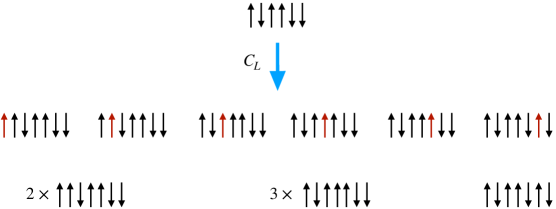
Figure 3: Illustration of contributions to $\langle\Psi|C_{L}^{\dagger}C_{L}|\Psi\rangle$. For $|\Psi\rangle$ we choose a zero magnetization state without any translational symmetry. Action of $C_{L}$ inserts spin up (in red) at $6$ different positions leading to a superposition of $3$ different states. Value of $\langle\Psi|C_{L}^{\dagger}C_{L}|\Psi\rangle$ is then directly related to the multiplicity of those states. In the example given we find $\langle\Psi|C_{L}^{\dagger}C_{L}|\Psi\rangle=2^{2}+3^{2}+1=14\geq 2L$ taking $\langle\Psi|\Psi\rangle=1$. The multiplicities are directly related to the lengths of the domains of spin ups present in the seed state. Denoting by $m$ the length of a domain to which we add a spin, the multiplicity of the resulting state is $m+1$. This is valid also for $m=0$ when we insert the spin up between the spin downs as on the right hand side of the figure.

Neel state and its generalizations:

Let us exemplify these concepts with direct computations for a simple case of a Neel state. The translationally invariant state is the combination

$$|\Psi_{0}\rangle=|\!\uparrow\downarrow\uparrow\downarrow\cdots\rangle+|\!\downarrow\uparrow\downarrow\uparrow\cdots\rangle,$$ (33)

and, up to a normalization, it can be generated by the action of $T_{L}$ on one of the two seed states, $|\!\uparrow\downarrow\uparrow\downarrow\cdots\rangle$ or $|\!\downarrow\uparrow\downarrow\uparrow\cdots\rangle$. By explicit computations we find $N_{\Psi_{0}}=2$. The Neel state has a partial translational invariance with the elementary cell given by either $|\!\uparrow\downarrow\rangle$ or $|\!\downarrow\uparrow\rangle$ for which we find $N_{\psi_{0}}=2$. In the case of the Neel state the bound (26) is actually saturated. The Neel state saturates also the bound $N_{\Psi_{0}}\geq 2$ for the product states of zero magnetization.

The Neel state can be generalized by taking alternatively domains of $m_{1}$ spin ups and $m_{2}$ spin downs. For a translationally invariant superposition of such states we find $\mathcal{N}_{m_{1},m_{2}}=(m_{1}^{2}+2m_{1}+m_{2})/(m_{1}+m_{2})$. When $m_{1}\neq m_{2}$ the state has finite magnetization and $N_{m_{1},m_{2}}$ can be smaller than $2$ — for example by taking $m_{2}$ much larger than $m_{1}$. However when $m=m_{1}=m_{2}$ (with the obvious condition $m\geq 1$) we find $\mathcal{N}_{m,m}=(m+3)/2\geq 2$ with equality only for $m=1$ which is again the Neel state.

III Adding a single spin to other 1D spin model ground states

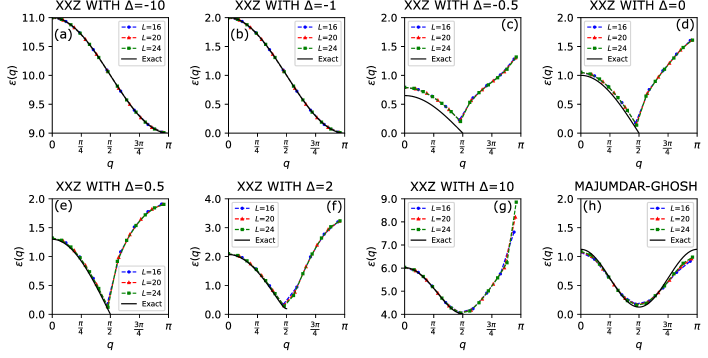
Figure 4: Dispersion relation $\varepsilon(q)$ of the excitation calculated using the same procedure as discussed in the main text of the paper for: (a-g) the XXZ model (34) with different values of the anisotropy $\Delta$, (h) the Majumdar-Ghosh model (35) that has the valence-bond solid as the ground state. Results for chains of various length $L$ are shown by symbols (the connecting dashed lines are guides to the eye). The thick black solid lines, for comparison purposes, show the exact analytical expressions: (a-g) for the XXZ model originating in the Bethe Ansatz, and (h) for the Majumdar-Ghosh model, see text for more details.

Here we show that the procedure, discussed in the main text works well also for other 1D spin models. [We note in passing a (successful) application of the procedure to the Shastry-Sutherland model discussed in Talstra and Strong (1997)]. To this end, we consider two models. The first is the XXZ model defined by

$$H^{\rm XXZ}_{L}=J\sum_{j=1}^{L}\left(\sigma^{x}_{j}\cdot\sigma^{x}_{j+1}+\sigma^{y}_{j}\cdot\sigma^{y}_{j+1}+\Delta\sigma^{z}_{j}\cdot\sigma^{z}_{j+1}\right),$$ (34)

where we set $J=1$ and widely vary the anisotropy $\Delta$ (cf. Talstra and Strong (1997) for the XY model result). The second is the Majumdar-Ghosh model with its Hamiltonian

$$H^{\rm MG}_{L}=J\sum_{j=1}^{L}\left(\vec{\sigma}_{j}\cdot\vec{\sigma}_{j+1}+\frac{1}{2}\vec{\sigma}_{j}\cdot\vec{\sigma}_{j+2}\right),$$ (35)

where again we set $J=1$.

The corresponding dispersions $\varepsilon(q)$ obtained through the procedure proposed in the main text, are shown in Fig. 4. For the XXZ model with easy axis anisotropy we observe perfect agreement with the results obtained using the Bethe Ansatz Caux et al. (2008); Franchini (2017); Bohrdt et al. (2018); Rutkevich (2022). The agreement is quantitatively worse for the XXZ model with an easy plane anisotropy: In this case more than one spinon is excited when a single spin is inserted in the ground state, cf. the XY limit discussed in Talstra and Strong (1997). For the Majumdar-Ghosh model only small deviations are observed from the exact dispersion, see Ref. Shastry and Sutherland (1981); Lavarélo and Roux (2014).

As a side note, in the Majumdar-Ghosh model the dispersion scales as $\propto q^{2}$ in the low-energy limit Shastry and Sutherland (1981); Bohrdt et al. (2018), despite having a ground state with valence bond character and thus the norm $N(q)$ nearly vanishing in an extended region of $|q|>\pi/2$, just as in Fig. 2(c2) of the main text. The conundrum is resolved by noting that in the Majumdar-Ghosh Hamiltonian Shastry and Sutherland (1981) there exist next-nearest-neighbor spin flip terms which lead to a $\propto\cos(2q)$ contribution to the dispersion relation.

References

- Khomskii (2010) D. I. Khomskii, Basic Aspects of the Quantum Theory of Solids: Order and Elementary Excitations (Cambridge University Press, Cambridge, 2010).
- Venema et al. (2016) L. Venema, B. Verberck, I. Georgescu, G. Prando, E. Couderc, S. Milana, M. Maragkou, L. Persechini, G. Pacchioni, and L. Fleet, Nat. Phys. 12, 1085 (2016).
- Auerbach (1994) A. Auerbach, Interacting Electrons and Quantum Magnetism (Springer-Verlag, New York, 1994).
- Bethe (1931) H. Bethe, Zeit. für Physik 71, 205 (1931).
- Faddeev and Takhtajan (1981) L. D. Faddeev and L. A. Takhtajan, Phys. Lett. A 85, 375 (1981).
- des Cloizeaux and Pearson (1962) J. des Cloizeaux and J. J. Pearson, Phys. Rev. 128, 2131 (1962).
- Tennant et al. (1993) D. A. Tennant, T. G. Perring, R. A. Cowley, and S. E. Nagler, Phys. Rev. Lett. 70, 4003 (1993).
- Lake et al. (2005) B. Lake, D. A. Tennant, C. D. Frost, and S. E. Nagler, Nature Materials 4, 329 (2005).
- Caux and Maillet (2005) J.-S. Caux and J. M. Maillet, Phys. Rev. Lett. 95, 077201 (2005).
- Klauser et al. (2011) A. Klauser, J. Mossel, J.-S. Caux, and J. van den Brink, Phys. Rev. Lett. 106, 157205 (2011).
- Schlappa et al. (2012) J. Schlappa, K. Wohlfeld, K. J. Zhou, M. Mourigal, M. W. Haverkort, V. N. Strocov, L. Hozoi, C. Monney, S. Nishimoto, S. Singh, A. Revcolevschi, J.-S. Caux, L. Patthey, H. M. Rønnow, J. van den Brink, and T. Schmitt, Nature 485, 82 (2012).
- Mourigal et al. (2013) M. Mourigal, M. Enderle, A. Klöpperpieper, J.-S. Caux, A. Stunault, and H. M. Rønnow, Nature Physics 9, 435 (2013).
- Ferrari et al. (2018) F. Ferrari, A. Parola, S. Sorella, and F. Becca, Phys. Rev. B 97, 235103 (2018).
- Sorella and Parola (1992) S. Sorella and A. Parola, Journal of Physics: Condensed Matter 4, 3589 (1992).
- Talstra and Strong (1997) J. C. Talstra and S. P. Strong, Phys. Rev. B 56, 6094 (1997).
- Penc et al. (1997) K. Penc, K. Hallberg, F. Mila, and H. Shiba, Phys. Rev. B 55, 15475 (1997).
- Penc and Serhan (1997) K. Penc and M. Serhan, Phys. Rev. B 56, 6555 (1997).
- Matveev et al. (2007a) K. A. Matveev, A. Furusaki, and L. I. Glazman, Phys. Rev. Lett. 98, 096403 (2007a).
- Matveev et al. (2007b) K. A. Matveev, A. Furusaki, and L. I. Glazman, Phys. Rev. B 76, 155440 (2007b).
- Vidal et al. (2003a) G. Vidal, J. I. Latorre, E. Rico, and A. Kitaev, Phys. Rev. Lett. 90, 227902 (2003a).
- Sato et al. (2006) J. Sato, M. Shiroishi, and M. Takahashi, Journal of Statistical Mechanics: Theory and Experiment 2006, P12017 (2006).
- Miwa and Smirnov (2019) T. Miwa and F. Smirnov, Letters in Mathematical Physics 109, 675 (2019).
- Murciano et al. (2020) S. Murciano, G. D. Giulio, and P. Calabrese, SciPost Phys. 8, 046 (2020).
- Niezgoda et al. (2020) A. Niezgoda, M. Panfil, and J. Chwedeńczuk, Phys. Rev. A 102, 042206 (2020).
- Alet et al. (2007) F. Alet, S. Capponi, N. Laflorencie, and M. Mambrini, Phys. Rev. Lett. 99, 117204 (2007).
- Korepin et al. (1993) V. E. Korepin, N. M. Bogoliubov, and A. G. Izergin, Quantum Inverse Scattering Method and Correlation Functions, Cambridge Monographs on Mathematical Physics (Cambridge University Press, 1993).
- Villain (1975) J. Villain, Physica B+C 79, 1 (1975).
- (28) See Supplemental Material at the end of the main text for details.
- Vidal et al. (2003b) G. Vidal, J. I. Latorre, E. Rico, and A. Kitaev, Phys. Rev. Lett. 90, 227902 (2003b).
- Keselman et al. (2020) A. Keselman, L. Balents, and O. A. Starykh, Phys. Rev. Lett. 125, 187201 (2020).
- Beekman et al. (2019) A. J. Beekman, L. Rademaker, and J. van Wezel, SciPost Phys. Lect. Notes , 11 (2019).
- Hagendorf and Liénardy (2017) C. Hagendorf and J. Liénardy, Journal of Physics A: Mathematical and Theoretical 50, 185202 (2017).
- Caux et al. (2008) J.-S. Caux, J. Mossel, and I. P. Castillo, Journal of Statistical Mechanics: Theory and Experiment 2008, P08006 (2008).
- Franchini (2017) F. Franchini, An Introduction to Integrable Techniques for One-Dimensional Quantum Systems, Vol. 940 (2017).
- Bohrdt et al. (2018) A. Bohrdt, D. Greif, E. Demler, M. Knap, and F. Grusdt, Phys. Rev. B 97, 125117 (2018).
- Rutkevich (2022) S. B. Rutkevich, Phys. Rev. B 106, 134405 (2022).
- Shastry and Sutherland (1981) B. S. Shastry and B. Sutherland, Phys. Rev. Lett. 47, 964 (1981).
- Lavarélo and Roux (2014) A. Lavarélo and G. Roux, The European Physical Journal B 87, 229 (2014).