Planck Constraints and Gravitational Wave Forecasts for
Primordial Black Hole Dark Matter Seeded by Multifield Inflation
Abstract
We perform a Markov Chain Monte Carlo (MCMC) analysis of a simple yet generic multifield inflation model characterized by two scalar fields coupled to each other and nonminimally coupled to gravity, fit to Planck 2018 cosmic microwave background (CMB) data. In particular, model parameters are constrained by data on the amplitude of the primordial power spectrum of scalar curvature perturbations on CMB scales , the spectral index , and the ratio of power in tensor to scalar modes , with a prior that the primordial power spectrum should also lead to primordial black hole (PBH) production sufficient to account for the observed dark matter (DM) abundance. We find that in particular controls the constraints on our model. Whereas previous studies of PBH formation from an ultra-slow-roll phase of inflation have highlighted the need for at least one model parameter to be highly fine-tuned, we identify a degeneracy direction in parameter space such that shifts by of one parameter can be compensated by comparable shifts in other parameters while preserving a close fit between model predictions and observations. Furthermore, we find this allowed parameter region produces observable gravitational wave (GW) signals in the frequency ranges to which upcoming experiments are projected to be sensitive, including Advanced LIGO and Virgo, the Einstein Telescope (ET), Cosmic Explorer (CE), DECIGO, and LISA.
I Introduction
Perhaps the most prominent and enduring puzzle in modern cosmology is the unknown nature of dark matter (DM), the predominant form of matter in the universe that is vital to structure formation and galactic stability. Primordial black holes (PBHs) Zel’dovich (1967); Hawking (1971); Carr and Hawking (1974); Meszaros (1974); Carr (1975); Khlopov et al. (1985); Niemeyer and Jedamzik (1999) have been posited to make up anywhere from less than a percent to the entirety of the DM abundance.
A leading candidate for a mechanism to seed PBH formation in the early universe is an amplification of the primordial spectrum of curvature perturbations. The typical mass with which PBHs form scales with the Hubble mass—the mass-energy contained within a Hubble sphere at the time of PBH formation—and hence PBHs could be a plausible explanation for a diverse range of phenomena. For example, a population of PBHs with could be relevant for various binary black hole merger events reported by LIGO-Virgo, whereas PBHs with could have served as seeds for the supermassive black holes at the centers of galaxies. On the other hand, if PBHs are to account for the entire observed DM abundance, then various theoretical and observational constraints limit the mass range for PBHs to a much lighter regime, with . See Refs. Khlopov (2010); Sasaki et al. (2018); Carr et al. (2021); Carr and Kühnel (2020); Green and Kavanagh (2021); Escrivà (2022); Villanueva-Domingo et al. (2021); Escrivà et al. (2022); Özsoy and Tasinato (2023) for recent reviews of PBHs and their current observational status.
Given the success of cosmic inflation as a model of the early universe, it is natural to turn to inflation as a mechanism to amplify the primordial power spectrum. The vast majority of work on PBHs formed after a phase of cosmic inflation has focused on single-field inflationary models. (See, e.g., the recent review article in Ref. Özsoy and Tasinato (2023) and references therein.) These constructions typically include ad hoc features in the inflationary potential , which could be better motivated in the context of additional fields, such as in the case of a step-feature model Inomata et al. (2022, 2021) or renormalization-group flow generated by interactions among several distinct fields Ezquiaga et al. (2018). Moreover, in such multifield models, it is generally not the case that a single scalar field can be isolated as the sole dynamical degree of freedom, with a mass hierarchy both above and below the scale of interest. Indeed, even the Standard Model of particle physics features four real scalars, namely the real components of the Higgs doublet, each of which remain in the spectrum at high energies in renormalizable gauges Mooij and Postma (2011); Greenwood et al. (2013); Kawai and Kim (2016). Finally, whereas single-field inflation models for PBH formation often appear finely-tuned and therefore ‘unnatural,’ there remains the possibility that such models may become natural when viewed from the perspective of a multifield model.
These considerations motivate the study of PBH formation directly in the context of multifield inflation. In a recent paper by the authors (Ref. Geller et al. (2022)), we demonstrated that PBHs relevant for DM will form from a realistic class of multifield inflationary models built from well-motivated high-energy ingredients. In particular, we considered inflationary models that incorporate multiple interacting scalar fields, each with a nonminimal gravitational coupling. Such models consist of generic mass-dimension-4 operators in an effective field theory (EFT) expansion of the action at inflationary energy scales, and (as discussed in Ref. Geller et al. (2022)) have a consistent ultraviolet completion in the context of supergravity. For various choices of model parameters, the inflationary dynamics in such models can include a phase of ultra-slow-roll evolution Garcia-Bellido and Ruiz Morales (2017); Ezquiaga et al. (2018); Germani and Prokopec (2017); Kannike et al. (2017); Motohashi and Hu (2017); Di and Gong (2018); Ballesteros and Taoso (2018); Pattison et al. (2017); Passaglia et al. (2019); Biagetti et al. (2018); Byrnes et al. (2019); Carrilho et al. (2019); Figueroa et al. (2021a); Inomata et al. (2022, 2021); Pattison et al. (2021); Balaji et al. (2022a, b); Kawai and Kim (2023); Karam et al. (2023); Pi and Sasaki (2022), which can yield PBHs with within the appropriate range to account for the entire DM abundance, while also matching high-precision measurements of the primordial perturbation spectrum on length-scales relevant for the cosmic microwave background radiation (CMB). In Ref. Geller et al. (2022), we demonstrated that eight distinct observational constraints—relating to both PBH and CMB observables—could be matched by adjusting only six free parameters in these models.
In this paper, we use a Markov Chain Monte Carlo (MCMC) analysis to systematically identify the regions of parameter space for the family of models constructed in Ref. Geller et al. (2022) that can produce relevant populations of PBHs for DM while continuing to match multiple observables related to the CMB. Our two-dimensional marginalized posterior distributions for pairs of parameters demonstrate that this general class of models can yield predictions for observables near the CMB pivot scale in close agreement with the latest observations Akrami et al. (2020a); Aghanim et al. (2020); Akrami et al. (2020b); Ade et al. (2021)—including the amplitude of the primordial power spectrum , the spectral tilt , and the ratio of power in tensor to scalar modes —while also producing PBHs with masses within the range for which they could account for the entire DM abundance. Such regions of parameter space also yield predictions for related observables that are easily compatible with the latest observational bounds, such as the running of the spectral index , the primordial isocurvature fraction , and local primordial non-Gaussianity .
In Ref. Geller et al. (2022), much as in previous studies of PBH formation from ultra-slow-roll evolution Garcia-Bellido and Ruiz Morales (2017); Ezquiaga et al. (2018); Germani and Prokopec (2017); Kannike et al. (2017); Motohashi and Hu (2017); Di and Gong (2018); Ballesteros and Taoso (2018); Pattison et al. (2017); Passaglia et al. (2019); Biagetti et al. (2018); Byrnes et al. (2019); Carrilho et al. (2019); Figueroa et al. (2021a); Inomata et al. (2022, 2021); Pattison et al. (2021), we found that one model parameter needed to be highly fine-tuned in order to match predictions for all eight relevant observables. As we will discuss here, with the aid of the MCMC we identify a degeneracy direction in parameter space such that shifts up to of any particular model parameter can be compensated by comparable shifts among the other parameters while preserving a close fit with observations. The overall tuning of each parameter required to match all the observables of interest, as measured by the posterior distributions for various ratios of parameters, is at the percent level, driven largely by the sub-percent-level accuracy to which the spectral index has been measured.
In addition to studying predictions from these models for CMB observables and PBH formation, we also analyze predictions for the amplification of primordial gravitational waves (GWs). GWs provide a tantalizing means to test the physics of the early universe. (For recent reviews, see Refs. Guzzetti et al. (2016); Caprini and Figueroa (2018); Domènech (2021).) In the context of PBH formation, the amplified spectrum of scalar curvature perturbations—necessary to induce gravitational collapse into PBHs—will source tensor modes beyond linear order in perturbation theory. Therefore PBH formation should be accompanied by a contribution to a stochastic GW background (SGWB) with a particular spectral shape Saito and Yokoyama (2009, 2010); Assadullahi and Wands (2010); Bugaev and Klimai (2010, 2011); Inomata and Nakama (2019).
Whereas the primordial GW spectrum is tightly constrained on scales near the CMB pivot scale , it is mostly unconstrained on the much shorter length-scales relevant for PBH formation. We calculate the expected contribution to the SGWB from PBH formation in our models, and find that the signal overlaps significantly with the (projected) integrated sensitivity curves for several next-generation detectors, including Advanced LIGO-Virgo (LIGO A+) Abbott et al. (2021), LISA Barausse et al. (2020), the Einstein Telescope (ET) Maggiore et al. (2020), Cosmic Explorer (CE) Reitze et al. (2019), and DECIGO Yuan and Huang (2021); Kawamura et al. (2021). These results suggest the exciting possibility that the production of DM in the form of PBHs from multifield models could soon be testable.
This paper is organized as follows. In § II, we introduce the multifield inflationary model and discuss dynamics during inflation. In § III, we discuss relevant physical observables predicted by the model. In § IV, we discuss how we constrain the allowed model parameter space. In § IV.2 we present our results and finally we conclude with further discussion in § VI. We discuss the effects of a phase of ultra-slow-roll evolution on the power spectrum of scalar curvature perturbations in Appendix A, and present additional details on the calculation of the induced GW spectrum in Appendix B.
II Multifield inflation model
Many types of single-field inflationary models yield predictions for CMB observables that are consistent with current observations. (See, e.g., Refs. Bassett et al. (2006); Martin et al. (2014); Guth et al. (2014); Akrami et al. (2020a).) Single-field models can also produce populations of PBHs relevant for DM Carr et al. (2021); Carr and Kühnel (2020); Green and Kavanagh (2021); Escrivà et al. (2022, 2022); Özsoy and Tasinato (2023); Kawai and Kim (2021); Ahmed et al. (2022). On the other hand, the Standard Model of particle physics includes multiple scalar degrees of freedom (at high energies in renormalizable gauges), and extensions beyond the Standard Model generically include many more Mooij and Postma (2011); Greenwood et al. (2013); Lyth and Riotto (1999); Mazumdar and Rocher (2011); Balaji et al. (2022c). We therefore focus on multifield models.
Likewise, nonminimal couplings in the effective action of the form , where is the spacetime Ricci scalar and is a dimensionless constant, are required for renormalization and are induced at one-loop even if the couplings vanish at tree level Callan, Jr. et al. (1970); Bunch et al. (1980); Bunch and Panangaden (1980); Birrell and Davies (1982); Parker and Toms (2009); Markkanen and Tranberg (2013); Kaiser (2016). The couplings generically increase with energy scale under renormalization-group flow with no UV fixed point Odintsov (1991); Buchbinder et al. (1992), and hence they can be large () at inflationary energy scales. Hence in this work we focus on models with multiple interacting scalar fields, each with a nonminimal coupling to gravity.
Such models are natural generalizations of the multifield models studied in Refs. Kaiser et al. (2013); Kaiser and Sfakianakis (2014); Schutz et al. (2014); Kaiser (2016), and are closely related to well-known models such as Higgs inflation Bezrukov and Shaposhnikov (2008); Greenwood et al. (2013); Kawai and Kim (2015, 2016) and -attractors Kallosh and Linde (2013a, b); Galante et al. (2015). In addition to providing an excellent fit to CMB observables, such models also feature efficient reheating Bezrukov et al. (2009); Garcia-Bellido et al. (2009); Child et al. (2013); DeCross et al. (2018a, b, c); Figueroa and Byrnes (2017); Repond and Rubio (2016); Ema et al. (2017); Sfakianakis and van de Vis (2019); Rubio and Tomberg (2019); Nguyen et al. (2019); van de Vis et al. (2020); Iarygina et al. (2020); Ema et al. (2021).
We restrict attention to spacetime dimensions and use metric signature . We also adopt natural units , within which the reduced Planck mass is .
II.1 Action and Equations of Motion
In the Jordan frame, the action for interacting scalar fields with , each with a nonminimal coupling to the spacetime Ricci scalar, is given by
| (1) |
where represents the nonminimal couplings, and tildes denote quantities in the Jordan frame. Upon performing the conformal transformation
| (2) |
we arrive at the Einstein-frame action Kaiser (2010)
| (3) |
The potential in the Einstein frame, , is related to the potential in the Jordan frame, ), by
| (4) |
In addition, the nonminimal couplings induce a nontrivial curvature of the field-space manifold in the Einstein frame, with metric given by
| (5) |
where . If more than one field has a nonminimal coupling to , then one cannot canonically normalize all of the fields while also retaining the simple Einstein-Hilbert term in the action Kaiser (2010).
To study the dynamics of background-order quantities and linearized fluctuations in such models, we adopt the gauge-invariant multifield formalism of Refs. Sasaki and Stewart (1996); Langlois and Renaux-Petel (2008); Peterson and Tegmark (2011a, b); Gong and Lee (2011); Gong and Tanaka (2011); Kaiser et al. (2013); DeCross et al. (2018a); Gong (2016), and consider perturbations around a spatially flat Friedmann-Lemaître-Robertson-Walker (FLRW) line element. Each scalar field may be decomposed into its vacuum expectation value and a spatially varying fluctuation,
| (6) |
The magnitude of the velocity of the background fields can be written as
| (7) |
so the unit vector in the direction of the fields’ velocity is given by
| (8) |
The covariant turn-rate vector is defined as
| (9) |
where for any field-space vector , and the covariant derivative employs the usual Levi-Civita connection associated with the field-space metric .
In terms of these quantities, the equations of motion for the background fields in the Einstein frame are
| (10) |
where and
| (11) |
Given the evolution of and , we can then calculate the slow-roll parameters,
| (12) |
Lastly, we may calculate the dimensionless power spectrum for the gauge-invariant scalar curvature perturbations , defined as
| (13) |
where indicates the end of inflation. As discussed in Ref. Geller et al. (2022), within the family of models we are considering, the fields generically evolve within a local minimum or “valley” of the potential in the Einstein frame, and therefore the isocurvature modes remain heavy throughout the duration of inflation, . Likewise, the covariant turn rate remains small, . (See also Refs. Kaiser et al. (2013); Kaiser and Sfakianakis (2014); Schutz et al. (2014); Kaiser (2016); DeCross et al. (2018a).) Under these conditions, when the background fields undergo ordinary slow-roll evolution with , the power spectrum assumes the form Gordon et al. (2000); Wands et al. (2002); Bassett et al. (2006); Kaiser et al. (2013); Geller et al. (2022)
| (14) |
with . As discussed in Appendix A, during ordinary slow-roll the modes remain frozen after crossing outside the Hubble radius, for , so one may evaluate for , where is the time when a mode of comoving wavenumber first crossed outside the Hubble radius during inflation:
| (15) |
Inflationary dynamics that yield a brief phase of ultra-slow-roll evolution, during which , will generate a spike in the power spectrum on corresponding wavenumbers . Such large-amplitude perturbations, in turn, can produce PBHs upon re-entering the Hubble radius after the end of inflation Garcia-Bellido and Ruiz Morales (2017); Ezquiaga et al. (2018); Germani and Prokopec (2017); Kannike et al. (2017); Motohashi and Hu (2017); Di and Gong (2018); Ballesteros and Taoso (2018); Pattison et al. (2017); Passaglia et al. (2019); Biagetti et al. (2018); Byrnes et al. (2019); Carrilho et al. (2019); Figueroa et al. (2021a); Inomata et al. (2022, 2021); Pattison et al. (2021). The main effect from ultra-slow-roll on the amplitude of the power spectrum is captured by the usual slow-roll expression in Eq. (14), given the relationship . Additional growth in for certain wavenumbers , beyond that represented by , can also occur during ultra-slow-roll. As discussed in Section IV.1, we have performed about 2 million simulations of the dynamics of this family of models across a broad region of parameter space. In order for this to be computationally tractable, we used the expression of Eq. (14) in our Markov Chain Monte Carlo analysis, which depends only on background-order quantities, and hence can be evaluated for a given point in parameter space very efficiently. In Appendix A, we bound the discrepancy in that can arise from the ultra-slow-roll phase in this family of models within the relevant regions of parameter space.
For discussion of possible effects from loop corrections on the power spectrum, compare Refs. Cheng et al. (2022); Kristiano and Yokoyama (2022, 2023); Choudhury et al. (2023a, b); Cheng et al. (2023) with Refs. Senatore and Zaldarriaga (2010, 2013a); Pimentel et al. (2012); Senatore and Zaldarriaga (2013b); Ando and Vennin (2021); Riotto (2023); Firouzjahi (2023); Motohashi and Tada (2023); Firouzjahi and Riotto (2023); Franciolini et al. (2023); Tasinato (2023).
II.2 Two-Field Model
Our aim is to include a generic set of mass-dimension-4 operators in the effective action for a two-field model. Even with only two fields, such models include a large number of free parameters. To help organize the couplings for each possible term, we adopt a supersymmetric framework, as in Ref. Geller et al. (2022). For the energy scales of interest, with during inflation, we may consider the global supersymmetry limit of supergravity.
We begin with a superpotential that includes only bilinear and trilinear couplings among two chiral superfields , where a tilde denotes quantities in the Jordan frame. Utilizing a shift-symmetric Kähler potential , as in countless supergravity inflation scenarios (see, e.g., Refs. McDonough and Scalisi (2016); Roest and Scalisi (2015)), one may easily construct models wherein the imaginary components of the scalar fields remain heavy during inflation, and hence effectively decouple. Upon relating the Jordan-frame potential for the real-valued scalar fields and to in the usual way, this supersymmetric framework yields an expression for of the form Geller et al. (2022)
| (16) | |||||
where has dimensions of mass and the parameters are dimensionless couplings. See Appendix B of Ref. Geller et al. (2022) for further details.
It is convenient to study the dynamics of our two-field model by adopting polar coordinates for the field space,
| (17) |
with and . Then the Jordan-frame potential can be written as
| (18) |
where
| (19) |
In addition to the couplings in the potential , the fields also have nonminimal couplings to gravity,
| (20) |
which are generated by the scalar fields’ self-interactions in a curved spacetime Callan, Jr. et al. (1970); Bunch et al. (1980); Bunch and Panangaden (1980); Birrell and Davies (1982); Odintsov (1991); Buchbinder et al. (1992); Faraoni (2001); Parker and Toms (2009); Markkanen and Tranberg (2013); Kaiser (2016). Upon performing the conformal transformation as in Eq. (2), the potential in the Einstein frame takes the form
| (21) |
in accord with Eq. (4).
II.3 Effective Single-Field Evolution
Whereas such models ostensibly include multiple interacting scalar fields, they generically exhibit dynamics that are effectively single-field. Following the conformal transformation, the effective potential in the Einstein frame generically develops local maxima (“ridges”) and local minima (“valleys”). Across a wide range of initial conditions and parameter values, dynamics in models with such potentials typically display an initial transient followed by effectively single-field evolution, along what has been dubbed a “single-field attractor” Kaiser et al. (2013); Kaiser and Sfakianakis (2014); Schutz et al. (2014); Kaiser (2016).
As in Ref. Geller et al. (2022), we impose additional symmetries among the couplings,
| (22) |
Imposing the symmetries of Eq. (22) yields at least two benefits: it reduces the dimensionality of the (still large) parameter space to explore, and it enables us to find analytic solutions for the direction in field space along which the fields evolve during inflation Geller et al. (2022). Moreover, upon imposing the symmetries of Eq. (22), the mass parameter only enters the dynamics in the combination , so we may set without loss of generality. Then the attractor dynamics during inflation—and hence predictions for observables—depend only on six free parameters: the five dimensionless couplings and one initial condition for the fields, . The only constraint on is that it be large enough to yield sufficient inflation, Kaiser et al. (2013); Kaiser and Sfakianakis (2014); Schutz et al. (2014); Geller et al. (2022). (Similar attractor behavior has been identified for other well-studied multifield models, such as hybrid inflation Clesse et al. (2009).)
Under the symmetry of Eq. (22), we also find that the Einstein-frame potential is invariant if we scale the parameters and fields as follows:
| (23) |
where is a real-valued constant. As field-space scalars, the potential and the angle are both invariant under the rescalings of Eq. (23). The metric , on the other hand, is a field-space tensor rather than a scalar, whose components do transform under these rescalings. The field-space curvature in these models falls as Kaiser et al. (2013); McDonough et al. (2020), and therefore the full inflationary dynamics—which depend on both and —become invariant under the rescalings of Eq. (23) in the limit .
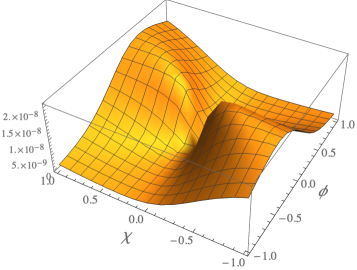
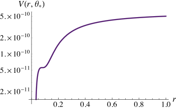
An example of a potential that yields appropriate inflationary dynamics and can also produce PBHs is given in Fig. 1; the parameters for this example are , , , , , and . The left panel shows the Einstein-frame potential , and the right panel shows the potential projected along the direction , corresponding to the single-field attractor evolution. The effective potential along the attractor direction has a local minimum and nearby local maximum at small field values, set by the condition Geller et al. (2022). Much as in single-field models Garcia-Bellido and Ruiz Morales (2017); Ezquiaga et al. (2018); Germani and Prokopec (2017); Kannike et al. (2017), such a feature in the potential can induce a brief phase of ultra-slow-roll evolution, generating a sharp spike in the power spectrum at specific wavenumbers Geller et al. (2022).
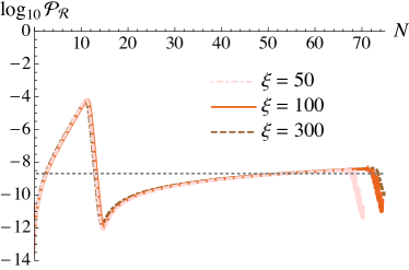
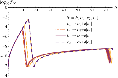
The power spectrum for the set of parameters used in Fig. 1 is shown in Fig. 2 as the dark orange line. To demonstrate the scaling relation of Eq. (23), we multiply the fiducial parameter set by appropriate factors of such that we obtain the scaled parameter sets corresponding to and . We further adjust by in each case, to accommodate the non-invariance of under the scaling relations of Eq. (23) for finite . The power spectra for these scaled parameters are also shown on Fig. 2; the curves are all nearly identical. Hence, given a set of parameters with some value of , we can use the scaling relation to find a corresponding set of parameters at a different value of that will yield the same predictions for observables. We will take advantage of this property to reduce the dimensionality of parameter space explored by the MCMC described in § IV.2.
III Observables
Upon imposing the symmetries between couplings given by Eq. (22), the two-field models under consideration are specified by five free dimensionless parameters, , and the fields’ initial value . Our aim is to determine how generically such models will satisfy CMB constraints, produce PBHs that could account for the DM abundance, and produce detectable GW signals.
We do so by determining the regions of parameter space that yield predictions that are consistent with both the empirical constraints and meet the criteria for producing PBHs. The latter—which yield a population of PBHs within the mass range of interest—are more restrictive, since by slightly relaxing these PBH constraints, the model generally remains in compliance with CMB observational constraints. In this section, we identify specific observables of interest and consider how model predictions for these observables vary with parameters.
III.1 Cosmic Microwave Background
The dimensionless power spectrum for the gauge-invariant curvature perturbations, , defined in Eq. (13), is central to the consideration of CMB constraints. In particular, predictions from this model must be consistent with the latest high-precision measurements of several quantities related to in the vicinity of the CMB pivot scale Akrami et al. (2020a); Aghanim et al. (2020); Akrami et al. (2020b); Ade et al. (2021), including the amplitude (or COBE normalization)
| (24) |
and the spectral index
| (25) |
where the second line holds to first order in slow-roll parameters, and are defined in Eq. (12), and is the time when crosses outside of the Hubble radius. We also consider the running of the spectral index,
| (26) |
Observables related to the CMB may be calculated using the expression in Eq. (14) in our model, across all the regions of parameter space under study here.
As noted in the previous section, within these models the fields evolve along single-field attractors during inflation, with exponentially suppressed turning within field space. In the limit , the tensor-to-scalar ratio for our multifield models reverts to its usual single-field form Bassett et al. (2006); Gong (2016); Kaiser et al. (2013); Geller et al. (2022)
| (27) |
Given that the isocurvature perturbations remain heavy and the turn rate remains suppressed in these models, we also find that typical multifield features, such as primordial isocurvature perturbations and primordial non-Gaussianity (parameterized by various dimensionless coefficients , corresponding to different shape functions for the bispectrum) remain exponentially suppressed Kaiser and Sfakianakis (2014); Kaiser (2016); Geller et al. (2022), easily consistent with the latest observations Akrami et al. (2020a, b).
We compare predictions from our model with the Planck 2018 results (when the spectral index is allowed to run with wavenumber) Akrami et al. (2020a) and the Planck-BICEP/Keck 2021 constraint on the tensor-to-scalar ratio Ade et al. (2021):
| (28) |
where the reported error bars correspond to confidence intervals.
III.2 Primordial Black Holes
The primordial power spectrum must exceed some threshold on appropriate scales in order for the curvature perturbations to seed primordial overdensities that will ultimately undergo gravitational collapse when these perturbations re-enter the Hubble radius after the end of inflation. For the models under consideration, this threshold is achieved for modes with that cross outside the Hubble radius during the transient period of ultra-slow roll. Typical estimates suggest a threshold for PBH formation of , about six orders of magnitude greater than the amplitude around the CMB pivot scale , Kühnel et al. (2016); Young et al. (2019); Kehagias et al. (2019); Escrivà et al. (2020); De Luca et al. (2020); Musco et al. (2021); Escrivà (2022).
Various effects beyond linear order in perturbation theory, such as stochastic dynamics and quantum diffusion, typically yield a non-Gaussian probability distribution function for curvature perturbations of various amplitudes, increasing the likelihood of large-amplitude perturbations compared to the Gaussian approximation. Such effects, in turn, can reduce the required threshold on by one to two orders of magnitude Ezquiaga et al. (2020); Figueroa et al. (2021a); Tada and Vennin (2022); Biagetti et al. (2021); Animali and Vennin (2022); Gow et al. (2022); Ferrante et al. (2023). Nevertheless, in this work we use the threshold ; this is conservative in that relaxing this threshold would only lead to a larger region of parameter space that would be consistent with observations. For computational tractability, we impose this conservative threshold via , given that when ultra-slow-roll effects are taken into account, as discussed further in Appendix A.
In addition to the peak height of the power spectrum, the PBHs that form after inflation are also sensitive to the time, during inflation, when the large-amplitude perturbations were first amplified and crossed outside the Hubble radius. We denote this time as
| (29) |
where is the number of -folds before the end of inflation when crossed outside the Hubble radius.
To determine an appropriate range for , we note that after the end of inflation, when perturbations of comoving wavenumber cross back inside the Hubble radius and induce gravitational collapse at time , the peak of the mass distribution scales with the Hubble mass as , with . (Here , where is the energy density contained with a Hubble sphere of radius .) One may then relate to Özsoy and Tasinato (2023)
| (30) |
where is the number of effectively massless degrees of freedom at the time of PBH formation. PBHs with in the range of interest for DM, Carr et al. (2021); Carr and Kühnel (2020); Green and Kavanagh (2021); Villanueva-Domingo et al. (2021); Escrivà (2022); Escrivà et al. (2022); Özsoy and Tasinato (2023), will therefore form from the collapse of perturbations with comoving wavenumber .
Next we evaluate the time between when the CMB pivot scale and modes of wavenumber each first crossed outside the Hubble radius:
| (31) |
where corresponds to the number of -folds before the end of inflation at which the pivot scale crossed the Hubble radius. In our models, the Hubble rate falls between and , with within the region of parameter space of interest. Taking into account the residual uncertainty on the duration of the reheating period Amin et al. (2014) we set , which yields
| (32) |
-folds before the end of inflation.
As discussed in Appendix A, setting is a conservative threshold, in that additional effects can only increase . For example, growth during the ultra-slow-roll phase modifies the peak wavenumber , yielding (and hence , where the “SR” quantities are evaluated in terms of the slow-roll expression in Eq. (14). Given these effects, in addition to the uncertainties from non-Gaussian effects and the reheating phase noted above, it is premature to plot a distribution of the resulting PBH masses or , since an uncertainty that increases by a few -folds reduces as per Eq. (31), which in turn increases as per Eq. (30). Instead, by imposing Eq. (32), we ensure that the region of our resulting parameter space that passes the threshold will produce PBHs large enough to avoid evaporation bounds.
III.3 Parameter Dependence & Degeneracies
Once the nonminimal coupling is fixed, the parameter space is described by the four remaining free parameters, . Varying these parameters changes the behavior of the potential and thus also changes predictions for , , and other observables in characteristic ways.
Measurements of CMB observables are sensitive to physics at the pivot scale, thus they will be affected by changes to the potential at large field values, that is, around . Meanwhile, the PBH constraints are largely sensitive to changes in the potential at small field values, around , corresponding to the period of ultra-slow roll during which the modes with first exit the Hubble radius. The tension is thus between tuning the small-field features to get a sufficiently large spike in to seed PBH formation without compromising the large-field dynamics. (See also Refs. Geller et al. (2022); Byrnes et al. (2019); Carrilho et al. (2019); Ando and Vennin (2021).)
In general, the longer the period of ultra-slow roll, that is, the larger the relative depth of the local minimum at small field values as compared to the local maximum and the large-field plateau, the larger the spike in the primordial power spectrum will be. There is a limit to this trend, however. If the relative depth of the local minimum is too large, the characteristic time for the fields to quantum tunnel out of the local minimum becomes comparable to the time for classical transit through the ultra-slow-roll region. In this instance, we cannot ignore the effects of quantum diffusion on the dynamics, hence, there is a range of parameters for which the fields undergo ultra-slow roll evolution long enough for PBHs to form post-inflation, but not so long that quantum effects become dominant. We can determine whether a potential will have a small-field feature that falls within this range by considering the magnitude of kinetic energy for the fields as they enter the ultra-slow-roll region. If the kinetic energy is too high, the fields will roll past the region of the potential for which too quickly for ultra-slow roll to yield a sufficient spike in , whereas if the kinetic energy is too low, the fields will become classically “stuck” in the local minimum. This is discussed in more detail in our previous work Geller et al. (2022).
Varying each of the parameters individually affects both the shape of the minimum/maximum feature at small field values as well as the slope of the potential between the large-field plateau and the local minimum, which will change the kinetic energy of the fields as they approach the region of the potential for which , as follows:
-
•
Increasing while keeping will both increase the relative depth of the local minimum while decreasing the slope of the potential as the fields approach the region with . The overall effect is to decrease the kinetic energy of the fields as they enter the ultra-slow roll regime.
-
•
Increasing also increases the relative depth of the local minimum, but increases the slope of the potential as the fields approach . The latter effect dominates, so the net result is to increase the kinetic energy of the fields.
-
•
Increasing both and will increase the kinetic energy of the fields as they approach the ultra-slow roll region.
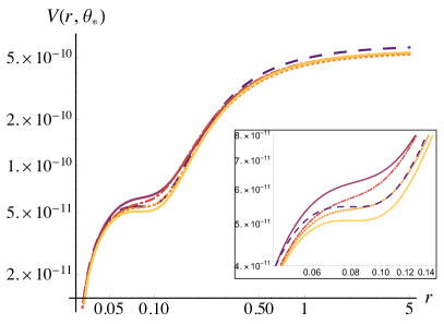
Thus the effect of parameter variations is such that increasing the magnitude of has the opposite effect to increasing the magnitudes of the . We find that the interplay of parameters is such that a certain sequence of small parameter variations will lead to a degenerate potential and power spectrum. An example of this is shown in Fig. 3. We begin at the fiducial parameter set and take a small step in the degeneracy direction given by the unit vector to a degenerate parameter set , where . The power spectrum is much more sensitive to the step size along the degeneracy direction than is the potential, so the right panel, for , uses , whereas the left panel, for , uses a step size of so that the effects of varying parameters can be more readily seen.
III.4 Gravitational Waves
In this work we also consider a complementary observable in inflationary PBH models, namely GWs sourced by the amplified curvature perturbation.
At second order in cosmological perturbation theory, scalar modes can source a SGWB. The induced GWs are usually described by the energy density per logarithmic frequency interval, normalized by the critical density (see, e.g., Ref. Domènech (2021))
| (33) |
Assuming that the GWs were induced by modes that crossed back inside the Hubble radius at a temperature during the radiation-dominated epoch, the fractional energy density today can be written as
| (34) |
where is the present value of the Hubble constant, , and is the GW spectral density at the time the waves were induced. The quantities and are the effective number of degrees of freedom for the radiation energy density and entropy; today, their values are equal to and . Using Aghanim et al. (2020) and , this becomes
| (35) |
The dimensionless spectral density when the modes are contained within the Hubble radius during the radiation-dominated epoch is given by
| (36) |
where the conformal time is defined as at horizon reentry in the radiation-dominated era, and the two respective polarization modes of GWs have been summed over. is the power spectrum of the induced tensor-mode perturbation sourced by linear scalar-mode perturbations at second order given by Eq. (B), which can be solved via the Green’s function method Ananda et al. (2007); Baumann et al. (2007) as
| (37) |
where are the two polarizations, is the Green’s function in radiation domination, and is the source term; detailed information is provided in Appendix B. The overline in Eq. (36) denotes an average over a few wavelengths for time oscillations led by the Green’s function. The GW spectrum induced by curvature perturbations is given by Kohri and Terada (2018); Domènech (2021)
| (38) |
where , , , and the appropriate kernel is given in Appendix B.
IV Planck Constraints on PBH-seeding Multifield Inflation
IV.1 Data and Likelihood
To constrain the model presented above, we use data from the Planck 2018 CMB temperature and polarization anisotropies and lensing spectra, and enforce a minimal requirement that the model can produce PBHs that could comprise all DM. We incorporate the CMB data using Gaussian priors corresponding to the Planck 2018 constraints on the CDM cosmological model. Specifically, we use measurements of the spectral index , the amplitude , and the running of the spectral index , corresponding to the marginalized parameter constraints in the context of the CDM model. We also enforce a one-sided Gaussian constraint on the tensor-to-scalar ratio corresponding to the combined Planck-BICEP/Keck observations. The best fit values for these quantities and their error bars are given in Eq. (28).
In order to translate these constraints to an inflation model, one must assume a reheating scenario; the CMB measurements are reported at the pivot scale , and calculating the time during inflation when this mode crossed the Hubble radius requires knowing the time spent during the reheating phase Dodelson and Hui (2003); Liddle and Leach (2003); Amin et al. (2014); Martin and Pinol (2021). If we assume that reheating is efficient and lasts for much less than one e-fold, then the CMB pivot scale for this model with typical parameters corresponds to Geller et al. (2022); however, the longer the reheating phase lasts, the smaller is. In inflationary models similar to the one that we consider, post-inflation reheating is typically efficient and lasts for -folds Bezrukov et al. (2009); Garcia-Bellido et al. (2009); Child et al. (2013); DeCross et al. (2018a, c, b); Figueroa and Byrnes (2017); Repond and Rubio (2016); Ema et al. (2017); Sfakianakis and van de Vis (2019); Nguyen et al. (2019); van de Vis et al. (2020); Iarygina et al. (2020); Ema et al. (2021); Figueroa et al. (2021b); Dux et al. (2022).
In our analysis, we allow to take on values within the range typically considered Akrami et al. (2020a), , and fix to optimize our reheat history. In other words, we choose to be the value between 50 and 60 such that the CMB observables at that scale most closely match the measurements listed in Eq. (28). An alternative approach would be to marginalize over the possible reheat histories; however, since this would make our MCMC computationally expensive, we choose to fix using this simpler procedure, wherein is treated as a derived parameter parameterizing the optimal reheating scenario. We leave a dedicated study of reheating dependence, e.g., in analogy to Ref. Martin et al. (2016), to future work.
To summarize, we take the model likelihood to be the following:
-
1.
A Gaussian over the Planck and BICEP/Keck observables, , corresponding to the Planck constraints on each of these quantities.
-
2.
A uniform likelihood for the peak of the power spectrum in the restricted range , namely the threshold to form PBHs, and zero likelihood for the peak falling below this.
-
3.
A uniform likelihood for the position of the peak of the power spectrum, in the restricted range , corresponding to the mass window where PBHs can comprise an fraction of DM, and zero likelihood outside of this range.
Next, in order to determine the observability of the induced GWs from curvature perturbations, we compare our predicted signals to the sensitivity curves from LISA Schmitz (2021), LIGO A+ Cahillane and Mansell (2022), the ET Maggiore et al. (2020), CE Reitze et al. (2019), and DECIGO Yagi and Seto (2011); Kawamura et al. (2021).
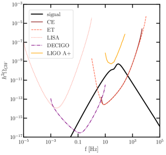
In Fig. 4, we show an example of a GW signal from our model with a particular set of parameters against these sensitivity curves.111Note that for plotting experimental sensitivities, we use power-law integrated sensitivity curves Thrane and Romano (2013). The power-law integrated curves will overlap with a SGWB when the signal-to-noise ratio (SNR) is greater than 1. Hence they are a better tool for visualizing the observability of a signal than the typically reported noise spectra. Given the total observation time and noise spectrum of an experiment , we can calculate the signal-to-noise ratio (SNR) of a background of GWs with power spectral density :
| (39) |
The SNR for this signal is maximal for CE at and also quite large for ET at , whereas in LIGO A+ and LISA, and finally in DECIGO the SNR is sizeable at .
The frequency limits for integration in the above expression, denoted , define the bandwidth of the detector. Eq. (39) therefore represents the total broadband SNR, integrated over both time and frequency. It can be computed as the expected SNR of a filtered cross-correlation. Here, in general one assumes that the SGWB is sufficiently described by a power-law of the from = where is the spectral index and is the reference frequency, which we set for example to Hz for ground-based detectors over the sensitivity region of interest. We set the observation times to the duration of data taking by the experiment. We can then use Eq. (39) to compute the value of GW amplitude required to reach a target SNR. In order to determine the detectability of the SGWB signal, we consider the spectrum from a particular inflationary model to be observable if it gives an SNR of .
IV.2 Results
We perform an MCMC analysis Foreman-Mackey et al. (2013) of our multifield inflation model fit to cosmological data as described in Sec. IV.1. The posterior sampling is performed using an ensemble sampler Goodman and Weare (2010) implemented in the Python package emcee Foreman-Mackey et al. (2013), with 200 walkers. We use the Python package Corner Foreman-Mackey (2016) for plotting results.
Given the scaling relationship in Eq. (23), we choose to fix and allow the remaining parameters , , , and to vary.222Whereas the dynamics of these models become independent of in the limit , we expect that data would not be able to constrain due to the scaling relations of Eq. (23), and the relative constraints on the other parameters would be comparable for any fixed value of . Hence we choose to fix to 100. We take broad uniform priors on the model parameters given by , , , .
We assess convergence of our MCMC chains by a combination of the autocorrelation time Goodman and Weare (2010); Foreman-Mackey et al. (2013) and stability of marginalized parameter constraints. The emcee documentation recommends running an analysis for 50 autocorrelation times to ensure convergence; however, this would be prohibitively computationally expensive for our case. On the other hand, as also noted in Ref. Foreman-Mackey et al. (2013), an accurate approximation to marginalized parameter constraints can be realized with significantly fewer samples. In total, we include approximately 1,300,000 samples for the final analysis, corresponding to an estimated 11 autocorrelation times. We find that as we vary the number of samples included in the analysis by 10%, the marginalized parameter constraints (central value and error bars) vary at the sub-percent level.
Constraints from requiring PBH DM
and satisfying Planck 2018 data
Parameter
Constraint
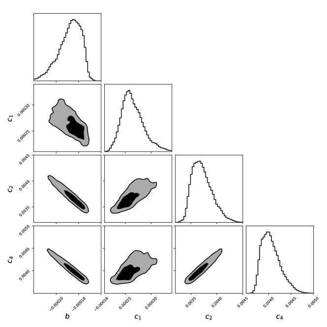
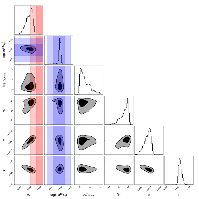
The main results of this analysis are shown in Table 1 and Figs. 5 and 6. Table 1 shows the marginalized posterior means, best-fit values, and corresponding error bars on model parameters, as well as the constraints on their ratios. The maximum likelihood model has , , , and , and yields predictions for CMB observables , , , and , in excellent compliance with Planck constraints. This demonstrates that there is a region of parameter space in our model that is both compatible with Planck constraints and can produce PBH DM.
The posterior distributions on the model parameters are shown in Fig. 5, and posterior distributions for derived (cosmological) parameters are shown in Fig. 6. Derived parameters are analyzed in post-processing of the MCMC chains, for a subset of samples. Consistent with emcee documentation Foreman-Mackey et al. (2013), we find the marginalized constraints on the model parameters from this subset of steps are near-identical to those from the full MCMC chains, thus validating our use of a subset of points for constraints on derived parameters, such as and .
From Fig. 5, we can clearly see the degeneracies discussed in § III.3. As expected, is anticorrelated with the other ’s, while all the parameters are positively correlated with one another. Moreover, at the larger end of the posterior distribution for , we see a sharp cutoff, whereas toward smaller values there is a more gradual tail. Due to the anticorrelation, this behavior is reversed for the ; the posteriors exhibit cutoffs at small values and a tail at larger values.
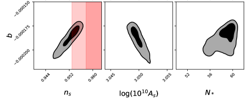
We can understand this behavior if we look at the marginalized posteriors for and the cosmological observables, a subset of which is shown in the last row of Fig. 5. The parameter shows a clear positive correlation with ; as we move along the contour to more negative values for , decreases past the Planck 2018 error bars. Hence, towards smaller values of (larger values of ), the posteriors show a tail corresponding to the Gaussian prior on the value of . There is also a correlation between and : larger values of produce models that prefer a larger . Hence at a large enough value for , we are eventually constrained by the requirement that be less than 60. This explains the sharp cut-offs observed in the posteriors.
We reiterate that the distributions of the , , , and the other observables shown in Figs. 5 and 6 are the optimal values for a given set of model parameters. That is, for a given set of model parameters, we consider the optimal reheat history, rather than marginalizing over possible reheat histories. From Fig. 6, one may appreciate that in comparison with the Planck measurement of , the (optimal) is essentially fixed in our model. Underlying this, however, is a delicate - compensation in the choice of , which in turn generates a spread of values (see, e.g., the posterior), in contrast to what one might expect if were solely driving the constraints on the models (which would lead to ). The optimization of reheat history is discussed further in Sec. IV.3.
In addition, although the resulting PBH masses tend to populate the lower end of the allowed DM window, , we find regions of parameter space that yield PBHs within that mass range. The tendency to produce lower mass black holes is driven by the Planck 2018 data; compliance with measurements at the pivot scale drives the parameters towards models with , which is consistent with the results of Ref. Geller et al. (2022). (See also Refs. Byrnes et al. (2019); Carrilho et al. (2019); Ando and Vennin (2021).) However, we emphasize that the estimation of the required range to obtain black holes in this window neglected the effects of non-Gaussianity in large-amplitude curvature perturbations, which would enhance power in large fluctuations and hence yield a higher probability of producing larger black holes Byrnes et al. (2012); Young and Byrnes (2013); Pattison et al. (2017); Biagetti et al. (2018); Kehagias et al. (2019); Ezquiaga et al. (2020); Ando and Vennin (2021); Tada and Vennin (2022); Biagetti et al. (2021); Ferrante et al. (2023). We leave incorporating these effects to future studies.
Finally, while the model parameters are constrained at the level, this is deceptive because of the strong degeneracies in parameter space. If we instead examine the ratios of the parameters, as shown in the bottom rows of Table 1, we see that these are constrained at the percent level. Hence, the parameters must be tuned to less than a percent in order for the model to produce an appropriate population of PBHs while also remaining in compliance with existing measurements.
IV.3 Degeneracy directions and compensations
As mentioned in Sec. III.3, we identify degeneracy directions in parameter space: directions along which parameter variations will leave the potential and power spectrum, and thus predictions for CMB observables, unchanged. In this section we study this quantitatively.
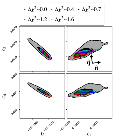
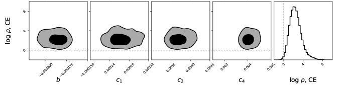
We consider two parameter sets to be degenerate if the difference of their total values is less than . We define five super-sets of degenerate points (parameter sets) within the parameter space, as illustrated in the scatter plots in Fig. 7 superposed upon four of the two-dimensional posteriors, in which each super-set is assigned a color: red, green, blue, magenta, and cyan. Parameter sets within a given color yield nearly identical values of ; parameter sets belonging to different colors yield different values of . The fiducial parameter set , used in the plots in Fig. 3, belongs to the set of red points in Fig. 7.
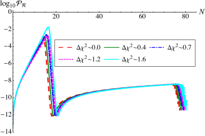
By computing the total relative to the red points, we can locally identify two directions within the parameter space. Along the degenerate direction , remains effectively constant (to within ). Along the orthogonal direction , changes appreciably, as shown in the legend of Fig. 7. The power spectra for five choices of parameters are plotted in Fig. 8, where each curve represents a single point from the super-set of corresponding color shown in Fig. 7.
Our analysis allows to vary within a range of -folds, and for a given parameter set, the ultimate fit to data is performed for the value of which minimizes ; we call this the optimal value. From the posterior in Fig. 6, we see that a larger value of , approaching the central Planck value, favors a smaller range of values for , whereas a smaller value of , moving away from the central Planck value, allows for a larger range of . Whereas we might expect the opposite behavior due to the scaling of the running with the size of , this behavior is in fact explained by looking at the trends in and as we move from the fiducial (red) set along the orthogonal direction . Here we use the notation to mean the normalized given by the square of the difference between the Planck and model value divided by the for observable .
The value of , where the difference is calculated relative to the fiducial parameter set , changes as: (red), (green), (blue), (magenta), and (cyan). These values almost exactly track the overall differences , for all but the cyan parameter set, showing that the change in is driven primarily by the fit to data. However, the optimal choice of is also somewhat driven by . At larger values of , i.e. closer to the Planck central value, the compensatory behavior of pushes it further from its Planck value, which results in an optimal choice of slightly below the value of 60 -folds that would minimize alone. This compensation between and results in a wider spread of optimal values for larger (closer to the Planck value) and a narrower spread for smaller (further from the Planck value). At smaller , is closer to the Planck value, and remains small for a wider range of values.
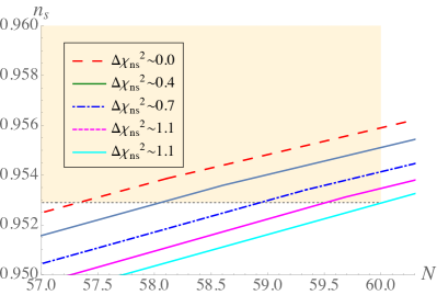
This interplay between values of and and the optimal value of can be seen by comparing the cyan and magenta curves in Fig. 9, which were chosen to have the same value of and thus equivalent , but which have different values of : for cyan and for magenta. As a result, the favored value is lower for the magenta parameter set (59.5) than for the cyan parameter set (60.0), indicating that the length of time for which the field experiences ultra slow-roll is longer for the cyan parameter set by about -folds. This is consistent with the fact that the cyan parameter set shown in Figs. 8-9 has a value of the coupling with larger magnitude than does the magenta parameter set. As we saw in Sec. III.3, increasing the magnitude of increases the depth of the local minimum in the small-field feature of the potential, and thus lengthens the duration of ultra-slow roll. This results in a modest but noticeable increase in the height of the peak in for cyan relative to magenta, as can be seen in Fig. 8. The interplay between and the optimal choice of thus connects the small-field physics to the CMB-scale physics.
V Gravitational Wave Forecasts
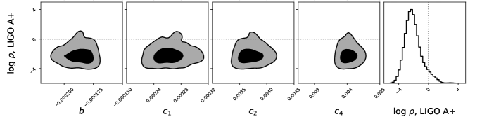
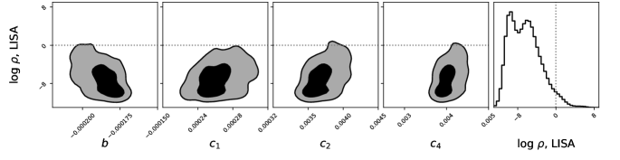
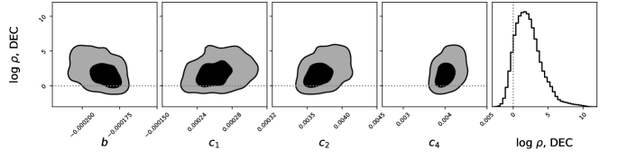
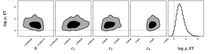
In the previous sections, we have discussed the 68% and 95% CL parameter regions for our multifield inflation model in terms of the parameters and , to obtain PBHs as all DM. This culminated in the marginalized constraints shown in § IV.2. Since inflationary models with large amplifications of scalar perturbations can also produce secondary tensor perturbations, we compute the GW spectra that result from these tensor perturbations in the present universe, using the allowed parameter space in § IV.2. We use the formulation described in III.4 to compute the dimensionless present-day spectral density of GW modes contained within the Hubble radius, , from Eq. (35) and the corresponding SNR, , as per Eq. (39) for various experiments. We describe in further detail the experiments and their sensitivities below.
At high frequencies, CE and ET are sensitive to the range - Hz. At slightly lower frequencies, between e.g. - Hz, we also expect LISA and DECIGO to have some sensitivity to the models we consider. It should be noted that at lower frequencies, data from the International Pulsar Timing Array (IPTA), which comes from a combination of three pulsar timing array experiments, can search for GWs in the frequency band - Hz. However, the multifield inflation models which produce PBHs that can comprise all of DM do not produce strong signals in this frequency range, hence we do not consider IPTA.
In Fig. 10, we show the SNR for the GWs from the sampled models in ET, CE, DECIGO, LISA, and LIGO A+. The dashed lines demarcate the threshold for observability where . We also list the mean for each experiment, along with 68% and 95% CL regions, in Table 2. ET, CE, and DECIGO are all very sensitive to the induced GWs from the sampled parameter region in Fig. 5, with most points yielding SNRs that are much larger than unity. For all three experiments, the centers of the posteriors lie at around . However, LISA and LIGO A+ have much less sensitivity for the favoured parameter region of Fig. 5. In the case of LISA, we see that only a very small part of the 95% confidence region lies above and for LIGO A+, we see that there is only a slightly larger, albeit small region lying above the threshold.
The peak sensitivity for each experiment can be understood in terms of the comoving wavenumbers that exit the Hubble radius during inflation, as well as the GW frequencies. For ET and CE, the peak sensitivity is around , where is the position of the hypothetical peak of the primordial power spectrum and is the comoving wavenumber that corresponds matter-radiation equality Aghanim et al. (2020). For DECIGO the peak lies at around and for LISA it is smaller still, at around . In our case, since producing PBHs as DM is an important physical requirement, we demand , which we recall from § III.2. For the resulting marginalized posterior distribution favoured for this model, we see that the is preferred, culminating in GWs favoured with frequencies lying in the mHz to kHz range; this is optimally situated for observation by ET, CE, and DECIGO. It should be noted that a very small region of the GW spectrum predicted by the posterior distribution is in the LIGO band. It has been shown that Gaussian density perturbations producing secondary GWs in the LIGO band produce PBHs that would have evaporated Kapadia et al. (2021). However, since there is an underestimation of as described at the end of § III.2 due to simplified assumptions, we confirm that the PBH mass would surpass the evaporation bound when propagating these effects. We intend to perform a detailed study of the PBH mass spectrum of which we leave to future work.
| Experiment | CL | CL | |
|---|---|---|---|
| LIGO A+ | |||
| LISA | |||
| ET | 2.04 | ||
| DECIGO | 1.91 | ||
| CE | 2.32 |
In summary, we find tantalizing GW phenomenology predicted for the posterior distribution of model parameters in our multifield inflation model. The correspondence between PBHs as DM and primordial GWs remains a compelling prospect for future ground- and space-based experiments.
VI Conclusions
We have performed an MCMC analysis of a simple yet generic multifield inflation model characterized by two fields coupled to each other and nonminimally coupled to gravity. This model was fit to Planck 2018 data, parametrized by measurements of the spectral parameters , , , and , and with a prior that the primordial power spectrum should lead to PBH production in the ultralight asteroid-mass range, where constraints still allow for PBHs to account for all of DM. We find a nontrivial region of parameter space in our model that is both compatible with Planck data and can produce PBH DM. The constraints on allowable regions of parameter space are driven in particular by and .
There are a number of reasons why we choose to focus on this multifield model. The Standard Model includes multiple scalar fields, and extensions to the Standard Model typically feature many more. Therefore, embeddings of inflationary dynamics within realistic models of high-energy physics are likely to involve multiple interacting scalar fields. Given that several types of single-field inflation models have successfully yielded predictions for PBHs as DM while remaining in compliance with CMB data Carr et al. (2021); Carr and Kühnel (2020); Green and Kavanagh (2021); Escrivà et al. (2022, 2022); Özsoy and Tasinato (2023), it seems natural to study whether multifield models can accomplish the same, while also reducing the necessary amount of fine-tuning to produce black holes. The family of models we consider is a natural generalization of multifield models that have been studied extensively in the literature Kaiser et al. (2013); Kaiser and Sfakianakis (2014); Schutz et al. (2014); Kaiser (2016), and is closely related to well-known examples such as Higgs inflation Bezrukov and Shaposhnikov (2008); Greenwood et al. (2013); Kawai and Kim (2015, 2016) and -attractors Kallosh and Linde (2013a, b); Galante et al. (2015).
The results of our MCMC show that there is a robust region of parameter space for which this family of models can produce PBHs in the appropriate mass range to comprise all of DM, while also remaining in compliance with Planck data. In particular, the posteriors on all parameters show a Gaussian-like tail at one end that is controlled by the measurement of , and a sharp cutoff at the other end from our requirement that remain in the range . Due to our procedure for optimizing over possible reheat scenarios, we find that the optimal typically fixes to the central value of the Planck measurement.
Through this analysis, we found that whereas the parameters of the model are constrained at around a 10% level, there is a degeneracy direction in the parameter space that leads to fine-tuned ratios at the percent level. It is possible that the actual required level of fine-tuning is greater than this, given that studies of single-field inflation models have found that model parameters typically need to be fine-tuned to as much as one part in in order to give rise to enhancements to the power spectrum that are sufficiently large to produce PBH DM Garcia-Bellido and Ruiz Morales (2017); Ezquiaga et al. (2018); Kannike et al. (2017); Germani and Prokopec (2017); Motohashi and Hu (2017); Di and Gong (2018); Ballesteros and Taoso (2018); Pattison et al. (2017); Passaglia et al. (2019); Byrnes et al. (2019); Biagetti et al. (2018); Carrilho et al. (2019); Inomata et al. (2022, 2021); Pattison et al. (2021). On the other hand, our results suggest that our multifield model may require less fine-tuning than some well-studied single-field models.
Upon fixing , predictions from our multifield model depend on only four free parameters. Moreover, we can shift any one of these parameters at the 10% level, and the constraints on the parameter ratios require the remaining three to be tuned at the 1% level, yielding a total degree of fine-tuning of approximately . However, since the most constraining quantity is , which has error bars at the 1% level, the relative amount of fine-tuning needed to produce PBHs is . While there exist more rigorous measures of fine-tuning Athron and Miller (2007); Fowlie (2014), we leave such a quantitative analysis to future work.
Furthermore, the allowed parameter region in this model produces observable GW signals in frequency ranges that future experiments such as LIGO A+ and Virgo, ET, CE, DECIGO and LISA are projected to be sensitive to. The observational prospects for DECIGO, ET, and CE are particularly good for this model; the latter two experiments have a central region of the MCMC posterior distribution with signal-to-noise ratio of . This result suggests that this inflation model is a viable and well-motivated candidate to explain both the observed DM and to generate observationally relevant primordial GWs.
Given these results, there are a number of interesting directions for future work. First, since we find that the spectral index is especially constraining for these models, it may be instructive to look at forecasts for constraints by CMB-S4 Abazajian et al. (2019, 2016). Moreover, improving measurements on the running of the spectral index could also play an important role in helping to distinguish among such models. In addition, predictions for the tensor-to-scalar ratio, , are approximately a factor of two below current observational bounds Ade et al. (2021), whereas similar models (with multiple interacting scalar fields and nonminimal couplings, but with no small-field features that could yield PBHs) tend to predict considerably smaller values, Kaiser and Sfakianakis (2014). Thus we expect measurements of to play a key role in future tests of this model. Along these same lines, it would be interesting to consider multifield models that combine the suppression of found in Ref. McDonough et al. (2020) with the enhancement on small scales studied here. We leave this for future work.
Second, in this work, we examined the SGWB resulting from inflation models that can produce PBHs as DM. It would also be interesting to perform a dedicated MCMC analysis to find the regions of parameter space for such models that produce detectable GWs, regardless of the implications for DM.
Third, given the discussion above of the amount of fine-tuning in our model, another direction one could pursue would be a Bayesian comparison of our model versus similar single-field models, or to further consider more rigorous quantitative measures of fine-tuning in these classes of models. (See, e.g., Ref. Cole et al. (2023).)
Finally, a more systematic analysis of uncertainties associated with the post-inflation reheating phase Martin and Pinol (2021) would be valuable for considering how the domain of viable parameter space for the multifield models studied here compares with those of other types of inflationary models. It is likely that if we were to sample within the range and then marginalize over it, that would increase the error bars in the estimates of our parameter constraints, which in turn would reduce the implied degree of fine-tuning for such models. Such questions remain a topic for further research.
Acknowledgements
We are pleased to thank Christian Byrnes, Philippa Cole, Alan Guth, Mikhail Ivanov, Benjamin Lehmann, Jérôme Martin, Subodh Patil, Salvatore Vitale, and Vincent Vennin for helpful discussions. This material is based upon work supported by the U.S. Department of Energy, Office of Science, Office of High Energy Physics of U.S. Department of Energy under grant Contract Number DE-SC0012567. W.Q. was additionally supported by National Science Foundation Graduate Research Fellowship under Grant Nos. 1745302 and 2141064. S.B. is supported by funding from the European Union’s Horizon 2020 research and innovation programme under grant agreement No. 101002846 (ERC CoG “CosmoChart”) as well as support from the Initiative Physique des Infinis (IPI), a research training program of the Idex SUPER at Sorbonne Universite. E.M. is supported in part by a Discovery Grant from National Sciences and Engineering Research Council of Canada.
Appendix A The power spectrum of scalar curvature perturbations during ultra-slow-roll
We may expand the spacetime line element to linear order in scalar metric perturbations around a spatially flat FLRW metric as in Ref. Bassett et al. (2006)
| (40) |
The metric functions , and are each gauge dependent, as are the field fluctuations identified in Eq. (6). We may construct the gauge-invariant curvature perturbation as the linear combination Bassett et al. (2006)
| (41) |
where , , and
| (42) |
with and defined in Eqs. (7)–(8). In a multifield model we may project onto the hypersurface of the field-space manifold that is orthogonal to the direction of the background fields’ motion via Kaiser et al. (2013)
| (43) |
in terms of which we may define the remaining gauge-invariant scalar perturbations
| (44) |
Although the field-space vector includes components, only are linearly independent. Moreover, where the field fluctuations are gauge dependent, the perturbations are gauge independent, up to linear order in fluctuations Kaiser et al. (2013).
In terms of these quantities, the derivative with respect to cosmic time of a mode is given by Kaiser et al. (2013)
| (45) |
Here is the covariant turn-rate vector defined in Eq. (9) and is the gauge-invariant Bardeen potential Bassett et al. (2006)
| (46) |
Upon using Eq. (10) for and Eq. (12) for , Eq. (45) is equivalent to
| (47) |
During ordinary slow-roll evolution of the background fields , with , we find the usual result that modes will remain conserved outside the Hubble radius, , in effectively single-field models, for which . Yet even in such (effectively) single-field scenarios, modes may undergo significant growth outside the Hubble radius during a phase of ultra-slow-roll evolution, as falls exponentially, . (See, e.g., Refs. Kinney (2005); Martin et al. (2013).)
In the limit , the equation of motion for modes assumes the simple form Bassett et al. (2006)
| (48) |
Using the definitions of the slow-roll parameters and in Eq. (12), this is equivalent to
| (49) |
During ultra-slow-roll, the slow-roll parameter falls rapidly, . In that limit, the amplitude of modes that have crossed outside the Hubble radius (with ) will grow whenever Kinney (2005); Martin et al. (2013); Byrnes et al. (2019); Liu et al. (2020); Cole et al. (2022). Near an inflection point of the potential, for which , the background equations of motion yield and hence . For small-field features in the potential of the sort we analyze here, however, need not vanish identically during the entire duration of ultra-slow-roll, and can exceed 3. More generally, need not remain constant during the ultra-slow-roll phase.
Given that the amplitude of modes can grow outside the Hubble radius while , departures from the typical slow-roll evolution are characterized by the quantity
| (50) |
where and indicate the start and end of the ultra-slow-roll phase, each determined by the times when crosses , and denotes the average of between and . Given that during ultra-slow-roll, and the duration of ultra-slow-roll (in -folds) may be approximated as .
The rapid fall of after the start of ultra-slow-roll means that some modes with wavenumber will become amplified after crossing outside the Hubble radius, beginning with wavenumber given by Liu et al. (2020)
| (51) |
where is the wavenumber of the mode that first exits the Hubble radius at the start of ultra-slow-roll. The value of comes from balancing the fall in amplitude of the “decaying” contribution to between the time that mode crosses outside the Hubble radius () and the onset of ultra-slow-roll (), with the growth of that same term during the ultra-slow-roll phase () Liu et al. (2020).
For modes with , which cross outside the Hubble radius prior to the onset of ultra-slow-roll, the power spectrum will be modified compared to the slow-roll expression of Eq. (14) as Liu et al. (2020) (see also Refs. Martin et al. (2013); Byrnes et al. (2019); Cole et al. (2022))
| (52) |
The steep growth begins at and reaches a peak at . For modes that exit the Hubble radius during ultra-slow-roll, with , the power spectrum falls from its peak at , since those modes merely oscillate prior to exiting the Hubble radius and then experience a shorter duration () of growth outside the Hubble radius during the remainder of the ultra-slow-roll phase. For modes that cross outside the Hubble radius later than , the background system again undergoes ordinary slow-roll evolution, so the standard expression for of Eq. (14) applies for Martin et al. (2013); Liu et al. (2020); Byrnes et al. (2019); Cole et al. (2022).
Incorporating the added growth of various modes during ultra-slow-roll, the dimensionless power spectrum reaches its maximum value at Martin et al. (2013); Liu et al. (2020); Byrnes et al. (2019); Cole et al. (2022):
| (53) |
The usual slow-roll expression for in Eq. (14) already incorporates parametric growth comparable to the term , given that and during ultra-slow-roll. This amplification matches the ultra-slow-roll amplification factor if during ultra-slow-roll. The main impacts of the ultra-slow-roll phase, compared to the usual slow-roll expression, are then twofold: the peak value can exceed the value represented by if ; and the wavenumber corresponding to the peak in shifts to shorter values compared to , due to the added growth of some modes after they cross outside the Hubble radius. In particular, whereas typically reaches its minimum value at and its maximum value at , the full expression for reaches its maximum value at Liu et al. (2020).
We may consider the impact of the ultra-slow-roll phase on for our family of models in typical regions of parameter space. We select a point among the red regions of Fig. 7, near our fiducial parameter set. For this set of parameters, the system enters ultra-slow-roll evolution (with ) at -folds before the end of inflation and exits ultra-slow-roll at , for a total duration -folds of ultra-slow-roll.
If we neglect the effects of ultra-slow-roll on the power spectrum, then the slow-roll approximation to the power spectrum reaches a peak value at , consistent with the behavior of most regions of parameter space under study here (see the posterior distribution of in Fig. 6). Given , this means that the slow-roll approximation to the power spectrum grows by a factor during the ultra-slow-roll phase, consistent with the parametric growth noted above: . For these parameters, meanwhile, the ultra-slow-roll amplification factor defined in Eq. (50) is . We thus find , which indicates that . In particular, the additional growth during the ultra-slow-roll phase yields , a factor greater than the peak predicted by the slow-roll approximate form .
Although details of the impact of ultra-slow-roll on depend on the model and parameter set under consideration, the growth of compared to that we find here is consistent with previous studies, which typically find Kinney (2005); Martin et al. (2013); Byrnes et al. (2019); Liu et al. (2020); Cole et al. (2022). Given that the majority of points in parameter space that we sampled in our MCMC analysis yield , we therefore conclude that additional growth from the ultra-slow-roll phase in this family of models is consistent with across most regions of parameter space, and hence should evade constraints (not incorporated here) based on overproducing PBHs, producing excessive spectral -distortions, and similar small-scale effects. (Evaluating such constraints typically requires moving beyond the approximation of a Gaussian probability distribution function for the scalar perturbations, and hence remains beyond the scope of our present analysis. See, e.g., Refs. Gow et al. (2021, 2022).)
Appendix B The power spectrum of induced tensor perturbations
We provide the complete equations for the computation of the tensor power spectrum used in Eq. (36). Let us begin with the definition of linear perturbations in the conformal Newtonian gauge for the metric of the form
| (54) |
where is the Newtonian potential and is the Bardeen curvature potential defined in Eq. (46), while , and are defined in Eq. (40). We define
| (55) |
which is the linear tensor perturbation including the two polarization modes. The transverse-traceless polarization tensors are
| (56) |
which are expressed in terms of orthonormal basis vectors and orthogonal to .
Keeping the tensor perturbation at linear order and the linear scalar perturbations up to second order, one can obtain the equation of motion for each polarization from the Einstein equation as
| (57) |
where second-order perturbations are projected away in the transverse-traceless decomposition Baumann et al. (2007) and we have neglected the anisotropic stress in the energy momentum tensor, so that , and thus
| (58) | ||||
| (59) |
where and determines the equation of state of the fluid that fills the universe, . The two internal momenta are given by and , and . The time evolution of the scalar potential is described by with respect to the primordial value , where the transfer function in the radiation-dominated universe is given in Ref. Domènech (2021).
The primordial Newtonian potential well outside the Hubble radius is related to the (gauge-invariant) curvature perturbation as , which yields
| (60) |
This is where parameters of the inflationary scenario given in § II enter the power spectrum of the tensor perturbation.
Solving the equation of motion of Eq. (57) by virtue of the Green’s function method of Eq. (37), we can compute the total power spectrum of the tensor perturbation as
| (61) |
It is convenient to use the dimensionless variables , and to rewrite the tensor spectrum as
| (62) | ||||
| (63) |
where our definition of coincides with that defined in Ref. Kohri and Terada (2018). Note that the projection of momentum under polarization tensors can be found in the Appendix B of Ref. Atal and Domènech (2021), where
| (64) |
For numerical evaluation, we adopt new variables , introduced in Ref. Kohri and Terada (2018), where , and the tensor spectrum now reads
| (65) | ||||
In the late-time limit of the radiation-dominated universe, that is, for and , we have the oscillation-averaged result from Ref. Kohri and Terada (2018):
| (66) | ||||
where is the usual Heaviside theta function. Hence the averaged analytical transfer function during radiation domination in Eq. (66) can be substituted into Eq. (65). The resulting integral will yield the oscillation-averaged power spectrum which can be substituted into Eq. (36), and the dimensionless GW background to be compared with experimental limits or signals can be determined. We have the calculation by direct comparison with the scale-invariant power spectrum normalized to unity (), which yields a dimensionless gravitational wave spectrum of as expected in Ref. Kohri and Terada (2018).
References
- Zel’dovich (1967) I. D. Zel’dovich, Ya.B.; Novikov, “The Hypothesis of Cores Retarded during Expansion and the Hot Cosmological Model,” Soviet Astron. AJ (Engl. Transl. ), 10, 602 (1967).
- Hawking (1971) Stephen Hawking, “Gravitationally collapsed objects of very low mass,” Mon. Not. Roy. Astron. Soc. 152, 75 (1971).
- Carr and Hawking (1974) Bernard J. Carr and S. W. Hawking, “Black holes in the early Universe,” Mon. Not. Roy. Astron. Soc. 168, 399–415 (1974).
- Meszaros (1974) P. Meszaros, “The behaviour of point masses in an expanding cosmological substratum,” Astron. Astrophys. 37, 225–228 (1974).
- Carr (1975) Bernard J. Carr, “The Primordial black hole mass spectrum,” Astrophys. J. 201, 1–19 (1975).
- Khlopov et al. (1985) M. Khlopov, B. A. Malomed, and Ia. B. Zeldovich, “Gravitational instability of scalar fields and formation of primordial black holes,” Mon. Not. Roy. Astron. Soc. 215, 575–589 (1985).
- Niemeyer and Jedamzik (1999) Jens C. Niemeyer and K. Jedamzik, “Dynamics of primordial black hole formation,” Phys. Rev. D 59, 124013 (1999), arXiv:astro-ph/9901292 .
- Khlopov (2010) Maxim Yu. Khlopov, “Primordial Black Holes,” Res. Astron. Astrophys. 10, 495–528 (2010), arXiv:0801.0116 [astro-ph] .
- Sasaki et al. (2018) Misao Sasaki, Teruaki Suyama, Takahiro Tanaka, and Shuichiro Yokoyama, “Primordial black holes—perspectives in gravitational wave astronomy,” Class. Quant. Grav. 35, 063001 (2018), arXiv:1801.05235 [astro-ph.CO] .
- Carr et al. (2021) Bernard Carr, Kazunori Kohri, Yuuiti Sendouda, and Jun’ichi Yokoyama, “Constraints on primordial black holes,” Rept. Prog. Phys. 84, 116902 (2021), arXiv:2002.12778 [astro-ph.CO] .
- Carr and Kühnel (2020) Bernard Carr and Florian Kühnel, “Primordial Black Holes as Dark Matter: Recent Developments,” Ann. Rev. Nucl. Part. Sci. 70, 355–394 (2020), arXiv:2006.02838 [astro-ph.CO] .
- Green and Kavanagh (2021) Anne M. Green and Bradley J. Kavanagh, “Primordial Black Holes as a dark matter candidate,” J. Phys. G 48, 043001 (2021), arXiv:2007.10722 [astro-ph.CO] .
- Escrivà (2022) Albert Escrivà, “PBH Formation from Spherically Symmetric Hydrodynamical Perturbations: A Review,” Universe 8, 66 (2022), arXiv:2111.12693 [gr-qc] .
- Villanueva-Domingo et al. (2021) Pablo Villanueva-Domingo, Olga Mena, and Sergio Palomares-Ruiz, “A brief review on primordial black holes as dark matter,” Front. Astron. Space Sci. 8, 87 (2021), arXiv:2103.12087 [astro-ph.CO] .
- Escrivà et al. (2022) Albert Escrivà, Florian Kuhnel, and Yuichiro Tada, “Primordial Black Holes,” (2022), arXiv:2211.05767 [astro-ph.CO] .
- Özsoy and Tasinato (2023) Ogan Özsoy and Gianmassimo Tasinato, “Inflation and Primordial Black Holes,” (2023), arXiv:2301.03600 [astro-ph.CO] .
- Inomata et al. (2022) Keisuke Inomata, Evan McDonough, and Wayne Hu, “Amplification of primordial perturbations from the rise or fall of the inflaton,” JCAP 02, 031 (2022), arXiv:2110.14641 [astro-ph.CO] .
- Inomata et al. (2021) Keisuke Inomata, Evan McDonough, and Wayne Hu, “Primordial black holes arise when the inflaton falls,” Phys. Rev. D 104, 123553 (2021), arXiv:2104.03972 [astro-ph.CO] .
- Ezquiaga et al. (2018) Jose Maria Ezquiaga, Juan Garcia-Bellido, and Ester Ruiz Morales, “Primordial Black Hole production in Critical Higgs Inflation,” Phys. Lett. B 776, 345–349 (2018), arXiv:1705.04861 [astro-ph.CO] .
- Mooij and Postma (2011) Sander Mooij and Marieke Postma, “Goldstone bosons and a dynamical Higgs field,” JCAP 09, 006 (2011), arXiv:1104.4897 [hep-ph] .
- Greenwood et al. (2013) Ross N. Greenwood, David I. Kaiser, and Evangelos I. Sfakianakis, “Multifield Dynamics of Higgs Inflation,” Phys. Rev. D 87, 064021 (2013), arXiv:1210.8190 [hep-ph] .
- Kawai and Kim (2016) Shinsuke Kawai and Jinsu Kim, “Multifield dynamics of supersymmetric Higgs inflation in SU(5) GUT,” Phys. Rev. D 93, 065023 (2016), arXiv:1512.05861 [hep-ph] .
- Geller et al. (2022) Sarah R. Geller, Wenzer Qin, Evan McDonough, and David I. Kaiser, “Primordial black holes from multifield inflation with nonminimal couplings,” Phys. Rev. D 106, 063535 (2022), arXiv:2205.04471 [hep-th] .
- Garcia-Bellido and Ruiz Morales (2017) Juan Garcia-Bellido and Ester Ruiz Morales, “Primordial black holes from single field models of inflation,” Phys. Dark Univ. 18, 47–54 (2017), arXiv:1702.03901 [astro-ph.CO] .
- Germani and Prokopec (2017) Cristiano Germani and Tomislav Prokopec, “On primordial black holes from an inflection point,” Phys. Dark Univ. 18, 6–10 (2017), arXiv:1706.04226 [astro-ph.CO] .
- Kannike et al. (2017) Kristjan Kannike, Luca Marzola, Martti Raidal, and Hardi Veermäe, “Single Field Double Inflation and Primordial Black Holes,” JCAP 09, 020 (2017), arXiv:1705.06225 [astro-ph.CO] .
- Motohashi and Hu (2017) Hayato Motohashi and Wayne Hu, “Primordial Black Holes and Slow-Roll Violation,” Phys. Rev. D 96, 063503 (2017), arXiv:1706.06784 [astro-ph.CO] .
- Di and Gong (2018) Haoran Di and Yungui Gong, “Primordial black holes and second order gravitational waves from ultra-slow-roll inflation,” JCAP 07, 007 (2018), arXiv:1707.09578 [astro-ph.CO] .
- Ballesteros and Taoso (2018) Guillermo Ballesteros and Marco Taoso, “Primordial black hole dark matter from single field inflation,” Phys. Rev. D 97, 023501 (2018), arXiv:1709.05565 [hep-ph] .
- Pattison et al. (2017) Chris Pattison, Vincent Vennin, Hooshyar Assadullahi, and David Wands, “Quantum diffusion during inflation and primordial black holes,” JCAP 10, 046 (2017), arXiv:1707.00537 [hep-th] .
- Passaglia et al. (2019) Samuel Passaglia, Wayne Hu, and Hayato Motohashi, “Primordial black holes and local non-Gaussianity in canonical inflation,” Phys. Rev. D 99, 043536 (2019), arXiv:1812.08243 [astro-ph.CO] .
- Biagetti et al. (2018) Matteo Biagetti, Gabriele Franciolini, Alex Kehagias, and Antonio Riotto, “Primordial Black Holes from Inflation and Quantum Diffusion,” JCAP 07, 032 (2018), arXiv:1804.07124 [astro-ph.CO] .
- Byrnes et al. (2019) Christian T. Byrnes, Philippa S. Cole, and Subodh P. Patil, “Steepest growth of the power spectrum and primordial black holes,” JCAP 06, 028 (2019), arXiv:1811.11158 [astro-ph.CO] .
- Carrilho et al. (2019) Pedro Carrilho, Karim A. Malik, and David J. Mulryne, “Dissecting the growth of the power spectrum for primordial black holes,” Phys. Rev. D 100, 103529 (2019), arXiv:1907.05237 [astro-ph.CO] .
- Figueroa et al. (2021a) Daniel G. Figueroa, Sami Raatikainen, Syksy Rasanen, and Eemeli Tomberg, “Non-Gaussian Tail of the Curvature Perturbation in Stochastic Ultraslow-Roll Inflation: Implications for Primordial Black Hole Production,” Phys. Rev. Lett. 127, 101302 (2021a), arXiv:2012.06551 [astro-ph.CO] .
- Pattison et al. (2021) Chris Pattison, Vincent Vennin, David Wands, and Hooshyar Assadullahi, “Ultra-slow-roll inflation with quantum diffusion,” JCAP 04, 080 (2021), arXiv:2101.05741 [astro-ph.CO] .
- Balaji et al. (2022a) Shyam Balaji, Joseph Silk, and Yi-Peng Wu, “Induced gravitational waves from the cosmic coincidence,” JCAP 06, 008 (2022a), arXiv:2202.00700 [astro-ph.CO] .
- Balaji et al. (2022b) Shyam Balaji, H. V. Ragavendra, Shiv K. Sethi, Joseph Silk, and L. Sriramkumar, “Observing Nulling of Primordial Correlations via the 21-cm Signal,” Phys. Rev. Lett. 129, 261301 (2022b), arXiv:2206.06386 [astro-ph.CO] .
- Kawai and Kim (2023) Shinsuke Kawai and Jinsu Kim, “Primordial black holes and gravitational waves from nonminimally coupled supergravity inflation,” Phys. Rev. D 107, 043523 (2023), arXiv:2209.15343 [astro-ph.CO] .
- Karam et al. (2023) Alexandros Karam, Niko Koivunen, Eemeli Tomberg, Ville Vaskonen, and Hardi Veermäe, “Anatomy of single-field inflationary models for primordial black holes,” JCAP 03, 013 (2023), arXiv:2205.13540 [astro-ph.CO] .
- Pi and Sasaki (2022) Shi Pi and Misao Sasaki, “Logarithmic Duality of the Curvature Perturbation,” (2022), arXiv:2211.13932 [astro-ph.CO] .
- Akrami et al. (2020a) Y. Akrami et al. (Planck), “Planck 2018 results. X. Constraints on inflation,” Astron. Astrophys. 641, A10 (2020a), arXiv:1807.06211 [astro-ph.CO] .
- Aghanim et al. (2020) N. Aghanim et al. (Planck), “Planck 2018 results. VI. Cosmological parameters,” Astron. Astrophys. 641, A6 (2020), [Erratum: Astron.Astrophys. 652, C4 (2021)], arXiv:1807.06209 [astro-ph.CO] .
- Akrami et al. (2020b) Y. Akrami et al. (Planck), “Planck 2018 results. IX. Constraints on primordial non-Gaussianity,” Astron. Astrophys. 641, A9 (2020b), arXiv:1905.05697 [astro-ph.CO] .
- Ade et al. (2021) P. A. R. Ade et al. (BICEP, Keck), “Improved Constraints on Primordial Gravitational Waves using Planck, WMAP, and BICEP/Keck Observations through the 2018 Observing Season,” Phys. Rev. Lett. 127, 151301 (2021), arXiv:2110.00483 [astro-ph.CO] .
- Guzzetti et al. (2016) M. C. Guzzetti, N. Bartolo, M. Liguori, and S. Matarrese, “Gravitational waves from inflation,” Riv. Nuovo Cim. 39, 399–495 (2016), arXiv:1605.01615 [astro-ph.CO] .
- Caprini and Figueroa (2018) Chiara Caprini and Daniel G. Figueroa, “Cosmological Backgrounds of Gravitational Waves,” Class. Quant. Grav. 35, 163001 (2018), arXiv:1801.04268 [astro-ph.CO] .
- Domènech (2021) Guillem Domènech, “Scalar Induced Gravitational Waves Review,” Universe 7, 398 (2021), arXiv:2109.01398 [gr-qc] .
- Saito and Yokoyama (2009) Ryo Saito and Jun’ichi Yokoyama, “Gravitational wave background as a probe of the primordial black hole abundance,” Phys. Rev. Lett. 102, 161101 (2009), [Erratum: Phys.Rev.Lett. 107, 069901 (2011)], arXiv:0812.4339 [astro-ph] .
- Saito and Yokoyama (2010) Ryo Saito and Jun’ichi Yokoyama, “Gravitational-Wave Constraints on the Abundance of Primordial Black Holes,” Prog. Theor. Phys. 123, 867–886 (2010), [Erratum: Prog.Theor.Phys. 126, 351–352 (2011)], arXiv:0912.5317 [astro-ph.CO] .
- Assadullahi and Wands (2010) Hooshyar Assadullahi and David Wands, “Constraints on primordial density perturbations from induced gravitational waves,” Phys. Rev. D 81, 023527 (2010), arXiv:0907.4073 [astro-ph.CO] .
- Bugaev and Klimai (2010) Edgar Bugaev and Peter Klimai, “Induced gravitational wave background and primordial black holes,” Phys. Rev. D 81, 023517 (2010), arXiv:0908.0664 [astro-ph.CO] .
- Bugaev and Klimai (2011) Edgar Bugaev and Peter Klimai, “Constraints on the induced gravitational wave background from primordial black holes,” Phys. Rev. D 83, 083521 (2011), arXiv:1012.4697 [astro-ph.CO] .
- Inomata and Nakama (2019) Keisuke Inomata and Tomohiro Nakama, “Gravitational waves induced by scalar perturbations as probes of the small-scale primordial spectrum,” Phys. Rev. D 99, 043511 (2019), arXiv:1812.00674 [astro-ph.CO] .
- Abbott et al. (2021) R. Abbott et al. (KAGRA, Virgo, LIGO Scientific), “Upper limits on the isotropic gravitational-wave background from Advanced LIGO and Advanced Virgo’s third observing run,” Phys. Rev. D 104, 022004 (2021), arXiv:2101.12130 [gr-qc] .
- Barausse et al. (2020) Enrico Barausse et al., “Prospects for Fundamental Physics with LISA,” Gen. Rel. Grav. 52, 81 (2020), arXiv:2001.09793 [gr-qc] .
- Maggiore et al. (2020) Michele Maggiore et al., “Science Case for the Einstein Telescope,” JCAP 03, 050 (2020), arXiv:1912.02622 [astro-ph.CO] .
- Reitze et al. (2019) David Reitze et al., “Cosmic Explorer: The U.S. Contribution to Gravitational-Wave Astronomy beyond LIGO,” Bull. Am. Astron. Soc. 51, 035 (2019), arXiv:1907.04833 [astro-ph.IM] .
- Yuan and Huang (2021) Chen Yuan and Qing-Guo Huang, “A topic review on probing primordial black hole dark matter with scalar induced gravitational waves,” (2021), arXiv:2103.04739 [astro-ph.GA] .
- Kawamura et al. (2021) Seiji Kawamura et al., “Current status of space gravitational wave antenna DECIGO and B-DECIGO,” PTEP 2021, 05A105 (2021), arXiv:2006.13545 [gr-qc] .
- Bassett et al. (2006) Bruce A. Bassett, Shinji Tsujikawa, and David Wands, “Inflation dynamics and reheating,” Rev. Mod. Phys. 78, 537–589 (2006), arXiv:astro-ph/0507632 .
- Martin et al. (2014) Jerome Martin, Christophe Ringeval, and Vincent Vennin, “Encyclopædia Inflationaris,” Phys. Dark Univ. 5-6, 75–235 (2014), arXiv:1303.3787 [astro-ph.CO] .
- Guth et al. (2014) Alan H. Guth, David I. Kaiser, and Yasunori Nomura, “Inflationary paradigm after Planck 2013,” Phys. Lett. B 733, 112–119 (2014), arXiv:1312.7619 [astro-ph.CO] .
- Kawai and Kim (2021) Shinsuke Kawai and Jinsu Kim, “Primordial black holes from Gauss-Bonnet-corrected single field inflation,” Phys. Rev. D 104, 083545 (2021), arXiv:2108.01340 [astro-ph.CO] .
- Ahmed et al. (2022) Waqas Ahmed, M. Junaid, and Umer Zubair, “Primordial black holes and gravitational waves in hybrid inflation with chaotic potentials,” Nucl. Phys. B 984, 115968 (2022), arXiv:2109.14838 [astro-ph.CO] .
- Lyth and Riotto (1999) David H. Lyth and Antonio Riotto, “Particle physics models of inflation and the cosmological density perturbation,” Phys. Rept. 314, 1–146 (1999), arXiv:hep-ph/9807278 .
- Mazumdar and Rocher (2011) Anupam Mazumdar and Jonathan Rocher, “Particle physics models of inflation and curvaton scenarios,” Phys. Rept. 497, 85–215 (2011), arXiv:1001.0993 [hep-ph] .
- Balaji et al. (2022c) Shyam Balaji, Guillem Domenech, and Joseph Silk, “Induced gravitational waves from slow-roll inflation after an enhancing phase,” (2022c), arXiv:2205.01696 [astro-ph.CO] .
- Callan, Jr. et al. (1970) Curtis G. Callan, Jr., Sidney R. Coleman, and Roman Jackiw, “A New improved energy - momentum tensor,” Annals Phys. 59, 42–73 (1970).
- Bunch et al. (1980) T. S. Bunch, P. Panangaden, and L. Parker, “On renormalization of field theory in curved space-time. I,” J. Phys. A 13, 901–918 (1980).
- Bunch and Panangaden (1980) T. S. Bunch and P. Panangaden, “On renormalization of field theory in curved space-time. II,” J. Phys. A 13, 919–932 (1980).
- Birrell and Davies (1982) N. D. Birrell and P. C. W. Davies, Quantum Fields in Curved Space (Cambridge Univ. Press, New York, 1982).
- Parker and Toms (2009) Leonard E. Parker and D. Toms, Quantum Field Theory in Curved Spacetime: Quantized Field and Gravity (Cambridge University Press, New York, 2009).
- Markkanen and Tranberg (2013) Tommi Markkanen and Anders Tranberg, “A Simple Method for One-Loop Renormalization in Curved Space-Time,” JCAP 08, 045 (2013), arXiv:1303.0180 [hep-th] .
- Kaiser (2016) David I. Kaiser, “Nonminimal Couplings in the Early Universe: Multifield Models of Inflation and the Latest Observations,” Fundam. Theor. Phys. 183, 41–57 (2016), arXiv:1511.09148 [astro-ph.CO] .
- Odintsov (1991) Sergei D. Odintsov, “Renormalization Group, Effective Action and Grand Unification Theories in Curved Space-time,” Fortsch. Phys. 39, 621–641 (1991).
- Buchbinder et al. (1992) I. L. Buchbinder, S. D. Odintsov, and I. L. Shapiro, Effective action in quantum gravity (1992).
- Kaiser et al. (2013) David I. Kaiser, Edward A. Mazenc, and Evangelos I. Sfakianakis, “Primordial Bispectrum from Multifield Inflation with Nonminimal Couplings,” Phys. Rev. D 87, 064004 (2013), arXiv:1210.7487 [astro-ph.CO] .
- Kaiser and Sfakianakis (2014) David I. Kaiser and Evangelos I. Sfakianakis, “Multifield Inflation after Planck: The Case for Nonminimal Couplings,” Phys. Rev. Lett. 112, 011302 (2014), arXiv:1304.0363 [astro-ph.CO] .
- Schutz et al. (2014) Katelin Schutz, Evangelos I. Sfakianakis, and David I. Kaiser, “Multifield Inflation after Planck: Isocurvature Modes from Nonminimal Couplings,” Phys. Rev. D 89, 064044 (2014), arXiv:1310.8285 [astro-ph.CO] .
- Bezrukov and Shaposhnikov (2008) Fedor L. Bezrukov and Mikhail Shaposhnikov, “The Standard Model Higgs boson as the inflaton,” Phys. Lett. B 659, 703–706 (2008), arXiv:0710.3755 [hep-th] .
- Kawai and Kim (2015) Shinsuke Kawai and Jinsu Kim, “Testing supersymmetric Higgs inflation with non-Gaussianity,” Phys. Rev. D 91, 045021 (2015), arXiv:1411.5188 [hep-ph] .
- Kallosh and Linde (2013a) Renata Kallosh and Andrei Linde, “Universality Class in Conformal Inflation,” JCAP 07, 002 (2013a), arXiv:1306.5220 [hep-th] .
- Kallosh and Linde (2013b) Renata Kallosh and Andrei Linde, “Non-minimal Inflationary Attractors,” JCAP 10, 033 (2013b), arXiv:1307.7938 [hep-th] .
- Galante et al. (2015) Mario Galante, Renata Kallosh, Andrei Linde, and Diederik Roest, “Unity of Cosmological Inflation Attractors,” Phys. Rev. Lett. 114, 141302 (2015), arXiv:1412.3797 [hep-th] .
- Bezrukov et al. (2009) F. Bezrukov, D. Gorbunov, and M. Shaposhnikov, “On initial conditions for the Hot Big Bang,” JCAP 06, 029 (2009), arXiv:0812.3622 [hep-ph] .
- Garcia-Bellido et al. (2009) Juan Garcia-Bellido, Daniel G. Figueroa, and Javier Rubio, “Preheating in the Standard Model with the Higgs-Inflaton coupled to gravity,” Phys. Rev. D 79, 063531 (2009), arXiv:0812.4624 [hep-ph] .
- Child et al. (2013) Hillary L. Child, John T. Giblin, Jr, Raquel H. Ribeiro, and David Seery, “Preheating with Non-Minimal Kinetic Terms,” Phys. Rev. Lett. 111, 051301 (2013), arXiv:1305.0561 [astro-ph.CO] .
- DeCross et al. (2018a) Matthew P. DeCross, David I. Kaiser, Anirudh Prabhu, C. Prescod-Weinstein, and Evangelos I. Sfakianakis, “Preheating after Multifield Inflation with Nonminimal Couplings, I: Covariant Formalism and Attractor Behavior,” Phys. Rev. D 97, 023526 (2018a), arXiv:1510.08553 [astro-ph.CO] .
- DeCross et al. (2018b) Matthew P. DeCross, David I. Kaiser, Anirudh Prabhu, Chanda Prescod-Weinstein, and Evangelos I. Sfakianakis, “Preheating after multifield inflation with nonminimal couplings, III: Dynamical spacetime results,” Phys. Rev. D 97, 023528 (2018b), arXiv:1610.08916 [astro-ph.CO] .
- DeCross et al. (2018c) Matthew P. DeCross, David I. Kaiser, Anirudh Prabhu, Chanda Prescod-Weinstein, and Evangelos I. Sfakianakis, “Preheating after multifield inflation with nonminimal couplings, II: Resonance Structure,” Phys. Rev. D 97, 023527 (2018c), arXiv:1610.08868 [astro-ph.CO] .
- Figueroa and Byrnes (2017) Daniel G. Figueroa and Christian T. Byrnes, “The Standard Model Higgs as the origin of the hot Big Bang,” Phys. Lett. B 767, 272–277 (2017), arXiv:1604.03905 [hep-ph] .
- Repond and Rubio (2016) Jo Repond and Javier Rubio, “Combined Preheating on the lattice with applications to Higgs inflation,” JCAP 07, 043 (2016), arXiv:1604.08238 [astro-ph.CO] .
- Ema et al. (2017) Yohei Ema, Ryusuke Jinno, Kyohei Mukaida, and Kazunori Nakayama, “Violent Preheating in Inflation with Nonminimal Coupling,” JCAP 02, 045 (2017), arXiv:1609.05209 [hep-ph] .
- Sfakianakis and van de Vis (2019) Evangelos I. Sfakianakis and Jorinde van de Vis, “Preheating after Higgs Inflation: Self-Resonance and Gauge boson production,” Phys. Rev. D 99, 083519 (2019), arXiv:1810.01304 [hep-ph] .
- Rubio and Tomberg (2019) Javier Rubio and Eemeli S. Tomberg, “Preheating in Palatini Higgs inflation,” JCAP 04, 021 (2019), arXiv:1902.10148 [hep-ph] .
- Nguyen et al. (2019) Rachel Nguyen, Jorinde van de Vis, Evangelos I. Sfakianakis, John T. Giblin, and David I. Kaiser, “Nonlinear Dynamics of Preheating after Multifield Inflation with Nonminimal Couplings,” Phys. Rev. Lett. 123, 171301 (2019), arXiv:1905.12562 [hep-ph] .
- van de Vis et al. (2020) Jorinde van de Vis, Rachel Nguyen, Evangelos I. Sfakianakis, John T. Giblin, and David I. Kaiser, “Time scales for nonlinear processes in preheating after multifield inflation with nonminimal couplings,” Phys. Rev. D 102, 043528 (2020), arXiv:2005.00433 [astro-ph.CO] .
- Iarygina et al. (2020) Oksana Iarygina, Evangelos I. Sfakianakis, Dong-Gang Wang, and Ana Achúcarro, “Multi-field inflation and preheating in asymmetric -attractors,” (2020), arXiv:2005.00528 [astro-ph.CO] .
- Ema et al. (2021) Yohei Ema, Ryusuke Jinno, Kazunori Nakayama, and Jorinde van de Vis, “Preheating from target space curvature and unitarity violation: Analysis in field space,” Phys. Rev. D 103, 103536 (2021), arXiv:2102.12501 [hep-ph] .
- Kaiser (2010) David I. Kaiser, “Conformal Transformations with Multiple Scalar Fields,” Phys. Rev. D 81, 084044 (2010), arXiv:1003.1159 [gr-qc] .
- Sasaki and Stewart (1996) Misao Sasaki and Ewan D. Stewart, “A General analytic formula for the spectral index of the density perturbations produced during inflation,” Prog. Theor. Phys. 95, 71–78 (1996), arXiv:astro-ph/9507001 .
- Langlois and Renaux-Petel (2008) David Langlois and Sebastien Renaux-Petel, “Perturbations in generalized multi-field inflation,” JCAP 04, 017 (2008), arXiv:0801.1085 [hep-th] .
- Peterson and Tegmark (2011a) Courtney M. Peterson and Max Tegmark, “Non-Gaussianity in Two-Field Inflation,” Phys. Rev. D 84, 023520 (2011a), arXiv:1011.6675 [astro-ph.CO] .
- Peterson and Tegmark (2011b) Courtney M. Peterson and Max Tegmark, “Testing Two-Field Inflation,” Phys. Rev. D 83, 023522 (2011b), arXiv:1005.4056 [astro-ph.CO] .
- Gong and Lee (2011) Jinn-Ouk Gong and Hyun Min Lee, “Large non-Gaussianity in non-minimal inflation,” JCAP 11, 040 (2011), arXiv:1105.0073 [hep-ph] .
- Gong and Tanaka (2011) Jinn-Ouk Gong and Takahiro Tanaka, “A covariant approach to general field space metric in multi-field inflation,” JCAP 03, 015 (2011), [Erratum: JCAP 02, E01 (2012)], arXiv:1101.4809 [astro-ph.CO] .
- Gong (2016) Jinn-Ouk Gong, “Multi-field inflation and cosmological perturbations,” Int. J. Mod. Phys. D 26, 1740003 (2016), arXiv:1606.06971 [gr-qc] .
- Gordon et al. (2000) Christopher Gordon, David Wands, Bruce A. Bassett, and Roy Maartens, “Adiabatic and entropy perturbations from inflation,” Phys. Rev. D 63, 023506 (2000), arXiv:astro-ph/0009131 .
- Wands et al. (2002) David Wands, Nicola Bartolo, Sabino Matarrese, and Antonio Riotto, “An Observational test of two-field inflation,” Phys. Rev. D 66, 043520 (2002), arXiv:astro-ph/0205253 .
- Cheng et al. (2022) Shu-Lin Cheng, Da-Shin Lee, and Kin-Wang Ng, “Power spectrum of primordial perturbations during ultra-slow-roll inflation with back reaction effects,” Phys. Lett. B 827, 136956 (2022), arXiv:2106.09275 [astro-ph.CO] .
- Kristiano and Yokoyama (2022) Jason Kristiano and Jun’ichi Yokoyama, “Ruling Out Primordial Black Hole Formation From Single-Field Inflation,” (2022), arXiv:2211.03395 [hep-th] .
- Kristiano and Yokoyama (2023) Jason Kristiano and Jun’ichi Yokoyama, “Response to criticism on ‘Ruling Out Primordial Black Hole Formation From Single-Field Inflation’: A note on bispectrum and one-loop correction in single-field inflation with primordial black hole formation,” (2023), arXiv:2303.00341 [hep-th] .
- Choudhury et al. (2023a) Sayantan Choudhury, Mayukh R. Gangopadhyay, and M. Sami, “No-go for the formation of heavy mass Primordial Black Holes in Single Field Inflation,” (2023a), arXiv:2301.10000 [astro-ph.CO] .
- Choudhury et al. (2023b) Sayantan Choudhury, Sudhakar Panda, and M. Sami, “No-go for PBH formation in EFT of single field inflation,” (2023b), arXiv:2302.05655 [astro-ph.CO] .
- Cheng et al. (2023) Shu-Lin Cheng, Da-Shin Lee, and Kin-Wang Ng, “Primordial perturbations from ultra-slow-roll single-field inflation with quantum loop effects,” (2023), arXiv:2305.16810 [astro-ph.CO] .
- Senatore and Zaldarriaga (2010) Leonardo Senatore and Matias Zaldarriaga, “On Loops in Inflation,” JHEP 12, 008 (2010), arXiv:0912.2734 [hep-th] .
- Senatore and Zaldarriaga (2013a) Leonardo Senatore and Matias Zaldarriaga, “On Loops in Inflation II: IR Effects in Single Clock Inflation,” JHEP 01, 109 (2013a), arXiv:1203.6354 [hep-th] .
- Pimentel et al. (2012) Guilherme L. Pimentel, Leonardo Senatore, and Matias Zaldarriaga, “On Loops in Inflation III: Time Independence of zeta in Single Clock Inflation,” JHEP 07, 166 (2012), arXiv:1203.6651 [hep-th] .
- Senatore and Zaldarriaga (2013b) Leonardo Senatore and Matias Zaldarriaga, “The constancy of in single-clock Inflation at all loops,” JHEP 09, 148 (2013b), arXiv:1210.6048 [hep-th] .
- Ando and Vennin (2021) Kenta Ando and Vincent Vennin, “Power spectrum in stochastic inflation,” JCAP 04, 057 (2021), arXiv:2012.02031 [astro-ph.CO] .
- Riotto (2023) A. Riotto, “The Primordial Black Hole Formation from Single-Field Inflation is Still Not Ruled Out,” (2023), arXiv:2303.01727 [astro-ph.CO] .
- Firouzjahi (2023) Hassan Firouzjahi, “One-loop Corrections in Power Spectrum in Single Field Inflation,” (2023), arXiv:2303.12025 [astro-ph.CO] .
- Motohashi and Tada (2023) Hayato Motohashi and Yuichiro Tada, “Squeezed bispectrum and one-loop corrections in transient constant-roll inflation,” (2023), arXiv:2303.16035 [astro-ph.CO] .
- Firouzjahi and Riotto (2023) Hassan Firouzjahi and Antonio Riotto, “Primordial Black Holes and Loops in Single-Field Inflation,” (2023), arXiv:2304.07801 [astro-ph.CO] .
- Franciolini et al. (2023) Gabriele Franciolini, Antonio Iovino, Junior., Marco Taoso, and Alfredo Urbano, “One loop to rule them all: Perturbativity in the presence of ultra slow-roll dynamics,” (2023), arXiv:2305.03491 [astro-ph.CO] .
- Tasinato (2023) Gianmassimo Tasinato, “A large approach to single field inflation,” (2023), arXiv:2305.11568 [hep-th] .
- McDonough and Scalisi (2016) Evan McDonough and Marco Scalisi, “Inflation from Nilpotent Kähler Corrections,” JCAP 11, 028 (2016), arXiv:1609.00364 [hep-th] .
- Roest and Scalisi (2015) Diederik Roest and Marco Scalisi, “Cosmological attractors from -scale supergravity,” Phys. Rev. D 92, 043525 (2015), arXiv:1503.07909 [hep-th] .
- Faraoni (2001) Valerio Faraoni, “A Crucial ingredient of inflation,” Int. J. Theor. Phys. 40, 2259–2294 (2001), arXiv:hep-th/0009053 .
- Clesse et al. (2009) Sebastien Clesse, Christophe Ringeval, and Jonathan Rocher, “Fractal initial conditions and natural parameter values in hybrid inflation,” Phys. Rev. D 80, 123534 (2009), arXiv:0909.0402 [astro-ph.CO] .
- McDonough et al. (2020) Evan McDonough, Alan H. Guth, and David I. Kaiser, “Nonminimal Couplings and the Forgotten Field of Axion Inflation,” (2020), arXiv:2010.04179 [hep-th] .
- Kühnel et al. (2016) Florian Kühnel, Cornelius Rampf, and Marit Sandstad, “Effects of Critical Collapse on Primordial Black-Hole Mass Spectra,” Eur. Phys. J. C 76, 93 (2016), arXiv:1512.00488 [astro-ph.CO] .
- Young et al. (2019) Sam Young, Ilia Musco, and Christian T. Byrnes, “Primordial black hole formation and abundance: contribution from the non-linear relation between the density and curvature perturbation,” JCAP 11, 012 (2019), arXiv:1904.00984 [astro-ph.CO] .
- Kehagias et al. (2019) Alex Kehagias, Ilia Musco, and Antonio Riotto, “Non-Gaussian Formation of Primordial Black Holes: Effects on the Threshold,” JCAP 12, 029 (2019), arXiv:1906.07135 [astro-ph.CO] .
- Escrivà et al. (2020) Albert Escrivà, Cristiano Germani, and Ravi K. Sheth, “Universal threshold for primordial black hole formation,” Phys. Rev. D 101, 044022 (2020), arXiv:1907.13311 [gr-qc] .
- De Luca et al. (2020) V. De Luca, G. Franciolini, and A. Riotto, “On the Primordial Black Hole Mass Function for Broad Spectra,” Phys. Lett. B 807, 135550 (2020), arXiv:2001.04371 [astro-ph.CO] .
- Musco et al. (2021) Ilia Musco, Valerio De Luca, Gabriele Franciolini, and Antonio Riotto, “Threshold for primordial black holes. II. A simple analytic prescription,” Phys. Rev. D 103, 063538 (2021), arXiv:2011.03014 [astro-ph.CO] .
- Ezquiaga et al. (2020) Jose María Ezquiaga, Juan García-Bellido, and Vincent Vennin, “The exponential tail of inflationary fluctuations: consequences for primordial black holes,” JCAP 03, 029 (2020), arXiv:1912.05399 [astro-ph.CO] .
- Tada and Vennin (2022) Yuichiro Tada and Vincent Vennin, “Statistics of coarse-grained cosmological fields in stochastic inflation,” JCAP 02, 021 (2022), arXiv:2111.15280 [astro-ph.CO] .
- Biagetti et al. (2021) Matteo Biagetti, Valerio De Luca, Gabriele Franciolini, Alex Kehagias, and Antonio Riotto, “The formation probability of primordial black holes,” Phys. Lett. B 820, 136602 (2021), arXiv:2105.07810 [astro-ph.CO] .
- Animali and Vennin (2022) Chiara Animali and Vincent Vennin, “Primordial black holes from stochastic tunnelling,” (2022), arXiv:2210.03812 [astro-ph.CO] .
- Gow et al. (2022) Andrew D. Gow, Hooshyar Assadullahi, Joseph H. P. Jackson, Kazuya Koyama, Vincent Vennin, and David Wands, “Non-perturbative non-Gaussianity and primordial black holes,” (2022), arXiv:2211.08348 [astro-ph.CO] .
- Ferrante et al. (2023) Giacomo Ferrante, Gabriele Franciolini, Antonio Iovino, Junior., and Alfredo Urbano, “Primordial non-Gaussianity up to all orders: Theoretical aspects and implications for primordial black hole models,” Phys. Rev. D 107, 043520 (2023), arXiv:2211.01728 [astro-ph.CO] .
- Amin et al. (2014) Mustafa A. Amin, Mark P. Hertzberg, David I. Kaiser, and Johanna Karouby, “Nonperturbative Dynamics Of Reheating After Inflation: A Review,” Int. J. Mod. Phys. D 24, 1530003 (2014), arXiv:1410.3808 [hep-ph] .
- Ananda et al. (2007) Kishore N. Ananda, Chris Clarkson, and David Wands, “The Cosmological gravitational wave background from primordial density perturbations,” Phys. Rev. D 75, 123518 (2007), arXiv:gr-qc/0612013 .
- Baumann et al. (2007) Daniel Baumann, Paul J. Steinhardt, Keitaro Takahashi, and Kiyotomo Ichiki, “Gravitational Wave Spectrum Induced by Primordial Scalar Perturbations,” Phys. Rev. D 76, 084019 (2007), arXiv:hep-th/0703290 .
- Kohri and Terada (2018) Kazunori Kohri and Takahiro Terada, “Semianalytic calculation of gravitational wave spectrum nonlinearly induced from primordial curvature perturbations,” Phys. Rev. D 97, 123532 (2018), arXiv:1804.08577 [gr-qc] .
- Dodelson and Hui (2003) Scott Dodelson and Lam Hui, “A Horizon ratio bound for inflationary fluctuations,” Phys. Rev. Lett. 91, 131301 (2003), arXiv:astro-ph/0305113 .
- Liddle and Leach (2003) Andrew R Liddle and Samuel M Leach, “How long before the end of inflation were observable perturbations produced?” Phys. Rev. D 68, 103503 (2003), arXiv:astro-ph/0305263 .
- Martin and Pinol (2021) Jérôme Martin and Lucas Pinol, “Opening the reheating box in multifield inflation,” JCAP 12, 022 (2021), arXiv:2105.03301 [astro-ph.CO] .
- Figueroa et al. (2021b) Daniel G. Figueroa, Adrien Florio, Toby Opferkuch, and Ben A. Stefanek, “Dynamics of Non-minimally Coupled Scalar Fields in the Jordan Frame,” (2021b), arXiv:2112.08388 [astro-ph.CO] .
- Dux et al. (2022) Frédéric Dux, Adrien Florio, Juraj Klarić, Andrey Shkerin, and Inar Timiryasov, “Preheating in Palatini Higgs inflation on the lattice,” (2022), arXiv:2203.13286 [hep-ph] .
- Martin et al. (2016) Jérôme Martin, Christophe Ringeval, and Vincent Vennin, “Information gain on reheating: The one bit milestone,” Phys. Rev. D 93, 103532 (2016).
- Schmitz (2021) Kai Schmitz, “New Sensitivity Curves for Gravitational-Wave Signals from Cosmological Phase Transitions,” JHEP 01, 097 (2021), arXiv:2002.04615 [hep-ph] .
- Cahillane and Mansell (2022) Craig Cahillane and Georgia Mansell, “Review of the Advanced LIGO Gravitational Wave Observatories Leading to Observing Run Four,” Galaxies 10, 36 (2022), arXiv:2202.00847 [gr-qc] .
- Yagi and Seto (2011) Kent Yagi and Naoki Seto, “Detector configuration of DECIGO/BBO and identification of cosmological neutron-star binaries,” Phys. Rev. D 83, 044011 (2011), [Erratum: Phys.Rev.D 95, 109901 (2017)], arXiv:1101.3940 [astro-ph.CO] .
- Thrane and Romano (2013) Eric Thrane and Joseph D. Romano, “Sensitivity curves for searches for gravitational-wave backgrounds,” Phys. Rev. D 88, 124032 (2013), arXiv:1310.5300 [astro-ph.IM] .
- Foreman-Mackey et al. (2013) Daniel Foreman-Mackey, David W. Hogg, Dustin Lang, and Jonathan Goodman, “emcee: The MCMC Hammer,” Publications of the Astronomical Society of the Pacific 125, 306 (2013), arXiv:1202.3665 [astro-ph.IM] .
- Goodman and Weare (2010) Jonathan Goodman and Jonathan Weare, “Ensemble samplers with affine invariance,” Communications in Applied Mathematics and Computational Science 5, 65–80 (2010).
- Foreman-Mackey (2016) Daniel Foreman-Mackey, “corner.py: Scatterplot matrices in python,” The Journal of Open Source Software 1, 24 (2016).
- Byrnes et al. (2012) Christian T. Byrnes, Edmund J. Copeland, and Anne M. Green, “Primordial black holes as a tool for constraining non-Gaussianity,” Phys. Rev. D 86, 043512 (2012), arXiv:1206.4188 [astro-ph.CO] .
- Young and Byrnes (2013) Sam Young and Christian T. Byrnes, “Primordial black holes in non-Gaussian regimes,” JCAP 08, 052 (2013), arXiv:1307.4995 [astro-ph.CO] .
- Kapadia et al. (2021) Shasvath J. Kapadia, Kanhaiya Lal Pandey, Teruaki Suyama, Shivaraj Kandhasamy, and Parameswaran Ajith, “Search for the Stochastic Gravitational-wave Background Induced by Primordial Curvature Perturbations in LIGO’s Second Observing Run,” Astrophys. J. Lett. 910, L4 (2021), arXiv:2009.05514 [gr-qc] .
- Athron and Miller (2007) Peter Athron and D. J. Miller, “A New Measure of Fine Tuning,” Phys. Rev. D 76, 075010 (2007), arXiv:0705.2241 [hep-ph] .
- Fowlie (2014) Andrew Fowlie, “CMSSM, naturalness and the ‘fine-tuning price’ of the Very Large Hadron Collider,” Phys. Rev. D 90, 015010 (2014), arXiv:1403.3407 [hep-ph] .
- Abazajian et al. (2019) Kevork Abazajian et al., “CMB-S4 Science Case, Reference Design, and Project Plan,” (2019), arXiv:1907.04473 [astro-ph.IM] .
- Abazajian et al. (2016) Kevork N. Abazajian et al. (CMB-S4), “CMB-S4 Science Book, First Edition,” (2016), arXiv:1610.02743 [astro-ph.CO] .
- Cole et al. (2023) Philippa S. Cole, Andrew D. Gow, Christian T. Byrnes, and Subodh P. Patil, “Primordial black holes from single-field inflation: a fine-tuning audit,” (2023), arXiv:2304.01997 [astro-ph.CO] .
- Kinney (2005) William H. Kinney, “Horizon crossing and inflation with large eta,” Phys. Rev. D 72, 023515 (2005), arXiv:gr-qc/0503017 .
- Martin et al. (2013) Jerome Martin, Hayato Motohashi, and Teruaki Suyama, “Ultra Slow-Roll Inflation and the non-Gaussianity Consistency Relation,” Phys. Rev. D 87, 023514 (2013), arXiv:1211.0083 [astro-ph.CO] .
- Liu et al. (2020) Jing Liu, Zong-Kuan Guo, and Rong-Gen Cai, “Analytical approximation of the scalar spectrum in the ultraslow-roll inflationary models,” Phys. Rev. D 101, 083535 (2020), arXiv:2003.02075 [astro-ph.CO] .
- Cole et al. (2022) Philippa S. Cole, Andrew D. Gow, Christian T. Byrnes, and Subodh P. Patil, “Steepest growth re-examined: repercussions for primordial black hole formation,” (2022), arXiv:2204.07573 [astro-ph.CO] .
- Gow et al. (2021) Andrew D. Gow, Christian T. Byrnes, Philippa S. Cole, and Sam Young, “The power spectrum on small scales: Robust constraints and comparing PBH methodologies,” JCAP 02, 002 (2021), arXiv:2008.03289 [astro-ph.CO] .
- Atal and Domènech (2021) Vicente Atal and Guillem Domènech, “Probing non-Gaussianities with the high frequency tail of induced gravitational waves,” JCAP 06, 001 (2021), arXiv:2103.01056 [astro-ph.CO] .