A Stochastic Approximate Expectation-Maximization for Structure Determination Directly from Cryo-EM Micrographs

Abstract

A single-particle cryo-electron microscopy (cryo-EM) measurement, called a micrograph, consists of multiple two-dimensional tomographic projections of a three-dimensional molecular structure at unknown locations, taken under unknown viewing directions. All existing cryo-EM algorithmic pipelines first locate and extract the projection images, and then reconstruct the structure from the extracted images. However, if the molecular structure is small, the signal-to-noise ratio (SNR) of the data is very low, and thus accurate detection of projection images within the micrograph is challenging. Consequently, all standard techniques fail in low-SNR regimes. To recover molecular structures from measurements of low SNR, and in particular small molecular structures, we devise a stochastic approximate expectation-maximization algorithm to estimate the three-dimensional structure directly from the micrograph, bypassing locating the projection images. We corroborate our computational scheme with numerical experiments, and present successful structure recoveries from simulated noisy measurements.

I Introduction

Cryo-electron microscopy (cryo-EM) is an increasingly popular technology in structural biology for elucidating the 3-D structure of biomolecules [nogales2016development, bai2015cryo]. In a cryo-EM experiment, individual copies of the target biomolecule are dispersed in a thin layer of vitreous ice. Then, a 2-D tomographic projection image, called a micrograph, is produced by an electron microscope [frank2006three]. A micrograph contains multiple tomographic projections of individual molecules, taken from unknown viewing directions and placed at unknown locations. Section II introduces the formation model of a micrograph in detail. The goal is to recover a 3-D molecular structure from a set of micrographs [elmlund2015cryogenic, cheng2015primer, sigworth2016principles, singer2020computational, bendory2020single].

The prevalent cryo-EM computational paradigm splits the reconstruction process into two main stages. The first stage consists of identifying and extracting the projection images from the micrographs. This stage is called particle picking, see for example [wang2016deeppicker, heimowitz2018apple, bepler2019positive, eldar2020klt]. In the second stage, the 3-D structure is reconstructed from the extracted projection images. Clearly, the quality of the reconstruction depends on the quality of the particle picking stage, which in turn depends heavily on the signal-to-noise ratio (SNR) of the micrograph [sigworth2004classical]. Therefore, this approach fails when the SNR of the micrograph is very low. In particular, it fails for small molecular structures that induce low SNR because fewer electrons carry information. The detection threshold has been recognized early on as a central limiting factor by the cryo-EM community; it was suggested that particle picking is impossible for molecules with molecular weight below $\sim 40\text{ kDa}$ [henderson1995potential, glaeser1999electron]. Indeed, to date, the vast majority of biomolecules whose structures have been determined using cryo-EM have molecular weights not smaller than $100\text{ kDa}$. Recovering smaller molecular structures is of crucial importance in cryo-EM, and is an active focal point of research endeavors in the field [wu2012fabs, danev2017expanding, scapin2018cryo, liu20193, zhang2019cryo, wu2020low, yeates2020development, bai2021seeing, wu2021cryo, zheng2022uniform].

The failure of the current cryo-EM computational paradigm to recover 3-D structures from low SNR micrographs can be understood through the lenses of classical estimation theory. Assume the 3-D volume is represented by $M$ parameters. Each particle projection is associated with five pose parameters—the 3-D rotation and the 2-D location. Thus, if we wish to jointly estimate the 3-D structure and the pose parameters of the $T$ projection images, like in older cryo-EM algorithms [harauz1983direct], the number of parameters to be estimated is $M+5T$, namely, grows linearly with the number of particle projections. In this case, it is well-known that the existence of a consistent estimator is not guaranteed; see for example the celebrated “Neyman-Scott paradox” [neyman1948consistent] and the multi-image alignment problem [aguerrebere2016fundamental]. Current approaches in cryo-EM can be thought of as “hybrid” in the sense that they estimate the locations of the particle projections in the particle picking stage (overall $2T$ parameters), and marginalize over the rotations (as well as over small translations relative to the estimated locations), see for example [scheres2012relion]. Thus, the number of parameters is $M+2T$, which still scales linearly with the number of projections. Indeed, as discussed above, this strategy is not consistent when the SNR is very low since particle picking fails. In this paper, we follow [bendory2023toward] and aim to marginalize over all nuisance variables—the locations and rotations. In this case, the number of parameters to be estimated is fixed and thus, given enough data, designing a consistent estimator might be feasible. Therefore, from an estimation theory view point, recovery in low SNR environments (and thus of small molecular structures) is potentially within reach.

The authors of [bendory2023toward] proposed to recover the 3-D volume directly from the micrographs using autocorrelation analysis, but their reported reconstructions were limited to low resolution. In this paper, we propose an alternative computational scheme for high resolution structure reconstruction based on the expectation-maximization (EM) algorithm [dempster1977maximum]. EM is an algorithm for finding a local maximum of a likelihood function with nuisance variables. It is widely used in many machine learning and statistics tasks, with applications to parameter estimation [feder1988parameter], mixture models [segol2021improved], deep belief networks [hinton2006fast], and independent component analsyis [hyvarinen2013independent], to name but a few. The EM algorithm was introduced to the cryo-EM community in [sigworth1998maximum], and is by now the most popular method for 3-D recovery from picked particles [scheres2012relion], where the 3-D rotations, but not the 2-D locations, are treated as nuisance variables.

Specifically, in order to recover the molecular structure directly from the micrograph, we aim to develop an EM algorithm that marginalizes over both 2-D translations and 3-D rotations. However, as we show in Section III-A, a direct application of EM is computationally intractable for our model since the number of possible projection locations in the micrograph grows quickly with the micrograph size. Therefore, based on [kreymer2022approximate, lan2020multi], we develop an EM algorithm that maximizes an approximation of the likelihood function. The computational complexity of the algorithm is linear in the micrograph size. To further accelerate the algorithm, we apply a stochastic variant of the approximate EM algorithm that linearly decreases the computational complexity and memory requirement of each iteration (at the potential cost of additional iterations); see Section III-C for further details.

In Section IV, we demonstrate that the proposed approximate EM can accurately estimate molecular structures from simulated data in various levels of noise, outperforming the autocorrelation analysis of [bendory2023toward]. This is inline with previous works on simpler 1-D and 2-D models [lan2020multi, kreymer2022approximate, bendory2017bispectrum, abbe2018multireference]. The SNR in the results of Section IV is around 1 (namely, the noise level and the power of the projection images are of the same order) due to the computational load of the algorithm (see Section III-E). Section LABEL:sec:conclusions outlines potential strategies to alleviating the computational complexity of our method so we can apply it to micrographs of extremely low SNR, as expected for reconstruction of small molecular structures. Crucially, our results do not depend, empirically, on the initial point of the algorithm. This suggests that our algorithm is less prone to model bias, where the output of the algorithm is biased by the initial model [sigworth2016principles]. Model bias has been recognized as a major pitfall of current cryo-EM algorithms [henderson2013avoiding].

II Measurement formation model

Our micrograph formation model follows the formulation of [bendory2023toward]. Let $f:\mathbb{R}^{3}\rightarrow\mathbb{R}$ represent the 3-D electrostatic potential of the molecule to be estimated. We refer to $f$ as the volume. A 2-D tomographic projection of the volume is a line integral, given by

$$I_{\omega}(x,y):=PR_{\omega}f=\int_{-\infty}^{\infty}\left(R_{\omega}f\right)(x,y,z)dz,$$ (1)

where the operator $R_{\omega}$ rotates the volume by  $\omega\in SO(3)$ and $P$ is the tomographic projection operator. The micrograph consists of $T$ tomographic projections, taken from different viewing directions $\left\{\omega_{t}\right\}_{t=1}^{T}\in SO(3)$, centered at different positions $\left\{\left(x_{t},y_{t}\right)\right\}_{t=1}^{T}$,

$$\mathcal{I}(x,y) =\int_{-\infty}^{\infty}\sum_{t=1}^{T}\left(R_{\omega_{t}}f\right)(x-x_{t},y-y_{t},z)dz+\varepsilon(x,y)$$

$$=\sum_{t=1}^{T}\int_{-\infty}^{\infty}\left(R_{\omega_{t}}f\right)(x-x_{t},y-y_{t},z)dz+\varepsilon(x,y)$$

$$=\sum_{t=1}^{T}I_{\omega_{t}}(x-x_{t},y-y_{t})+\varepsilon(x,y),$$ (2)

where $\varepsilon(x,y)$ is assumed to be i.i.d. white Gaussian noise with zero mean and variance $\sigma^{2}$.

We further assume that the micrograph is discretized on a Cartesian grid, the particle projections are centered on the grid, and each projection is of size $L\times L$ pixels; the projection size, $L$, is assumed to be known. We denote the indices on the grid by $\vec{\ell}=(\ell_{x},\ell_{y})\in\mathbb{Z}^{2}$. Thus, our micrograph model $\mathcal{I}\in\mathbb{R}^{N\times N}$ reads

$$\mathcal{I}[\vec{\ell}]=\sum_{t=1}^{T}I_{\omega_{t}}[\ell_{x}-\ell_{x_{t}},\ell_{y}-\ell_{y_{t}}]+\varepsilon[\vec{\ell}].$$ (3)

The goal is to estimate $f$ from several micrographs while the rotations, translations, and the number of projections are unknown. Importantly, it is possible to reconstruct the target volume only up to a 3-D rotation, a 3-D translation, and a reflection. Similar mathematical models were thoroughly studied in previous works for one- and two-dimensional setups [bendory2019multi, lan2020multi, marshall2020image, bendory2023multi, kreymer2022two, shalit2022generalized, kreymer2022approximate]. Fig. 1 presents an example of a noisy micrograph $\mathcal{I}$ at different SNRs, where

$$\operatorname{SNR}:=\frac{\mathbb{E}\left[\lVert I_{\omega_{t}}\rVert_{\text{F}}^{2}\right]}{L^{2}\sigma^{2}}\approx\frac{\frac{1}{T}\sum_{t=1}^{T}\lVert I_{\omega_{t}}\rVert_{\text{F}}^{2}}{L^{2}\sigma^{2}},$$ (4)

where $\lVert\cdot\rVert_{\text{F}}$ is the Frobenius norm. Section LABEL:sec:conclusions discusses how to include additional aspects of the cryo-EM reconstruction problem in the proposed technique, such as the effect of the contrast transfer function (CTF) [erickson1971measurement], colored noise, and non-uniform distribution of the rotations of the particles over $SO(3)$.

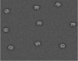
(a)

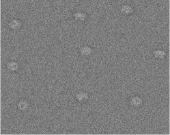
(b)

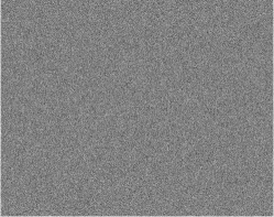
(c)

Figure 1: Three micrographs at different SNRs. Each measurement contains $T=9$ projections of the target volume. We focus on the low SNR regime, in which the 2-D locations and 3-D rotations of the projection images cannot be estimated reliably.

Following previous works [marshall2020image, bendory2023multi], we also assume that each translation is separated by at least a full projection length, $L$, from its neighbors, in both the horizontal and vertical axes. Explicitly,

$$|\ell_{x_{t}}-\ell_{x_{s}}|\geq 2L-1\text{ and }|\ell_{y_{t}}-\ell_{y_{s}}|\geq 2L-1,\text{ for all }t\neq s.$$ (5)

In Section LABEL:subsec:arbitrary_spacing_distribution, we discuss the implications of mitigating this constraint by allowing the projection images to be arbitrarily close.

II-A Volume formation model

Let $f$ be the Coulomb potential representing the molecule, which is smooth and real-valued. Its 3-D Fourier transform, $\hat{f}$, is finitely expanded by

$$\hat{f}(ck,\theta,\varphi)=\sum_{\ell=0}^{\ell_{\text{max}}}\sum_{m=-\ell}^{\ell}\sum_{s=1}^{S(\ell)}x_{\ell,m,s}Y_{\ell}^{m}(\theta,\varphi)j_{\ell,s}(k),\quad k\leq 1,$$ (6)

where $c$ is the bandlimit, $S(\ell)$ is determined using the Nyquist criterion as described in [zhang2021anisotropic], $j_{\ell,s}$ is the normalized spherical Bessel function, given by

$$j_{\ell,s}(k)=\frac{4}{\lvert j_{\ell+1}(u_{\ell,s})\rvert}j_{\ell}(u_{\ell,s}k),$$ (7)

where $j_{\ell}$ is the spherical Bessel function of order $\ell$, $u_{\ell,s}$ is the $s$-th positive zero of $j_{\ell}$, and $Y_{\ell}^{m}$ is the complex spherical harmonic, defined by

$$Y_{\ell}^{m}(\theta,\varphi):=\sqrt{\frac{2\ell+1}{4\pi}\frac{(\ell-m)!}{(\ell+m)!}}P_{\ell}^{m}(\cos\theta)e^{im\varphi},$$ (8)

where $P_{\ell}^{m}$ are the associated Legendre polynomials with the Condon-Shortley phase. We set $c=1/2$ for sampling at the Nyquist rate [levin20183d]. Under this model, we aim to estimate the expansion coefficients $x_{\ell,m,s}$ that describe $f$. Since $f$ is real-valued, $\hat{f}$ is conjugate-symmetric and thus the expansion coefficients satisfy $x_{\ell,-m,s}=(-1)^{\ell+m}\overline{x_{\ell,m,s}}$.

Let $I_{\omega}$ denote the tomographic projection obtained from viewing direction $\omega\in SO(3)$. By the Fourier projection-slice theorem (see, e.g., [natterer2001mathematics]), its 2-D Fourier transform is given by

$$\widehat{I}_{\omega}(ck,\varphi)=\sum_{\ell,m,m^{\prime},s}x_{\ell,m,s}D_{m^{\prime},m}^{\ell}(\omega)Y_{\ell}^{m^{\prime}}\left(\frac{\pi}{2},\varphi\right)j_{\ell,s}(k),$$ (9)

where $D_{m^{\prime},m}^{\ell}(\omega)$ is a Wigner-D matrix. Note that the projection images in the micrograph model (3) are expressed in the space domain, whereas (9) is expressed in Fourier space. To bridge this gap, we use the prolate spheroidal wave functions (PSWFs) [slepian1964prolate] as explained next.

II-B Expressing the projection image in space domain using the prolate spheroidal wave functions

The PSWFs are eigenfunctions of the truncated Fourier transform:

$$\alpha_{N,n}\psi_{N,n}(\textbf{k})=\int_{\|\textbf{r}\|_{2}\leq 1}\psi_{N,n}(\textbf{r})e^{ic(\textbf{r}\cdot\textbf{k})}d\textbf{r},$$ (10)

where $c$ is the bandlimit of the eigenfunction $\psi_{N,n}$. The eigenfunctions are orthonormal on the unit disk $\mathbb{D}:=\left\{\textbf{r}\in\mathbb{R}^{2},\lVert\textbf{r}\rVert_{2}\leq 1\right\}$, and they are the most energy concentrated among all $c$-bandlimited functions on $\mathbb{D}$, i.e., they satisfy

$$\psi_{N,n}(\textbf{r})=\operatorname*{arg\,max}_{\psi}\frac{\lVert\psi(\textbf{r})\rVert_{\mathcal{L}^{2}(\mathbb{D})}}{\lVert\psi(\textbf{r})\rVert_{\mathcal{L}^{2}(\mathbb{R}^{2})}}.$$ (11)

Explicitly, the PSWFs are given in polar coordinates by

$$\psi_{N,n}(r,\varphi)=\begin{cases}\frac{1}{\sqrt{8\pi}}\alpha_{N,n}R_{N,n}(r)e^{iN\varphi},&r\leq 1,\\ 0,&r>1,\end{cases}$$ (12)

where the range of $N\in\mathbb{Z}$, $n\in\mathbb{N}\cup\{0\}$ is determined by [landa2017steerable, Eq. (8)], the $R_{N,n}$ are a family of real, one-dimensional functions, defined explicitly in [landa2017steerable, Eq. (66)], and $\alpha_{N,n}$ is the eigenvalue corresponding to the $(N,n)$-th PSWF (10). From (12), we can also see that the PSWFs are steerable [freeman1991design]—rotating the image is equivalent to multiplying the eigenfunction $\psi_{N,n}$ by a phase dependent only on the rotation and the index $N$. The indices $N$ and $n$ are referred to, respectively, as the angular index and the radial index.

We may expand the projection (9) in Fourier domain using the PSWFs:

$$\widehat{I}_{\omega}(ck,\theta)=\sum_{N,n}b_{N,n}(\omega)\psi_{N,n}(k,\theta).$$ (13)

The coefficients are given by

$$b_{N,n}(\omega)$$

$$=\frac{4}{\sqrt{2\pi}\lvert\alpha_{N,n}\rvert^{2}}\int_{0}^{2\pi}\int_{0}^{1}\widehat{I}_{\omega}(ck,\theta)R_{N,n}(k)e^{-iN\theta}kdkd\theta$$

$$=\sum_{l,m^{\prime},m,s}x_{\ell,m,s}\frac{\sqrt{8\pi}}{\alpha_{N,n}}Y_{\ell}^{m^{\prime}}\left(\frac{\pi}{2},0\right)D_{m^{\prime},m}^{\ell}(\omega)$$

$$\times\frac{1}{2\pi}\int_{0}^{2\pi}e^{i(m^{\prime}-N)\theta}d\theta\int_{0}^{1}j_{\ell,s}(k)R_{N,n}(k)kdk$$

$$=\sum_{\ell\geq\lvert N\rvert}\sum_{m,s}x_{\ell,m,s}D_{N,m}^{\ell}(\omega)\beta_{\ell,s;N,n},$$ (14)

where

$$\beta_{\ell,s;N,n}:=\frac{\sqrt{8\pi}}{\alpha_{N,n}}Y_{\ell}^{N}(\pi/2,0)\int_{0}^{1}j_{\ell,s}(k)R_{N,n}(k)kdk$$ (15)

for $\ell\geq\lvert N\rvert$, and $0$ otherwise.

$$I_{\omega}(r,\varphi) =\left(\frac{c}{2\pi}\right)^{2}\sum_{\ell=0}^{\ell_{\text{max}}}\sum_{N=-\ell}^{\ell}\sum_{m=-\ell}^{\ell}\sum_{n=0}^{n_{\text{max}}(N)}\sum_{s=1}^{S(\ell)}x_{\ell,m,s}\alpha_{N,n}\beta_{\ell,s;N,n}D_{N,m}^{\ell}(\omega)\psi_{N,n}(r,\varphi)$$

$$:=\sum_{\ell=0}^{\ell_{\text{max}}}\sum_{N=-\ell}^{\ell}\sum_{m=-\ell}^{\ell}\sum_{n=0}^{n_{\text{max}}(N)}\sum_{s=1}^{S(\ell)}x_{\ell,m,s}\widehat{\beta}_{\ell,s;N,n}D_{N,m}^{\ell}(\omega)\psi_{N,n}(r,\varphi)$$ (16)

Using the property (10), we can express the projection in space domain as (II-B), where $n_{\text{max}}$ is chosen according to [landa2017steerable, Eq. (8)], and $\widehat{\beta}_{\ell,s;N,n}:=\left(\frac{c}{2\pi}\right)^{2}\alpha_{N,n}\beta_{\ell,s;N,n}$.

Using (3) and (II-B), we can now relate the parameters of the volume directly with the micrograph, bypassing the particle picking stage. In the following section, we present our scheme for estimating the coefficients $x_{\ell,m,s}$ from a set of noisy micrographs.

III An approximate expectation-maximization (EM) algorithm for cryo-EM

III-A Approximate EM

The EM algorithm estimates the maximum of a likelihood function by iteratively applying the expectation (E) and the maximization (M) steps [dempster1977maximum]. For the model (3), given a measurement $\mathcal{I}$, the maximum likelihood estimator (MLE) is the maximizer of $p(\mathcal{I};x)$ for the vector of coefficients $x$ (6). The 2-D translations and 3-D rotations associated with the projection images within the micrograph are treated in our analysis as nuisance variables. In the EM terminology, they are dubbed unobserved or latent variables.

In the E-step of the $(k+1)$-th iteration of the EM algorithm, one computes $Q(x;x_{k})$—the expectation of the complete log-likelihood function, where $x_{k}$ is the current estimate of the parameters and the expectation is taken over all admissible configurations of translations and rotations. However, for our model, the number of possible translations in the micrograph grows quickly with the micrograph size, $N^{2}$. Consequently, a direct application of EM is computationally intractable. Instead, we follow [lan2020multi, kreymer2022approximate] and partition the micrograph $\mathcal{I}$ into $N_{\text{patches}}=(N/L)^{2}$ non-overlapping patches $\{\mathcal{I}_{p}\}_{p=1}^{N_{\text{patches}}}$; each patch is of the size of a projection image $L\times L$. In EM terminology, the patches are dubbed the observed data. The separation condition (5) implies that each patch $\mathcal{I}_{p}$ can contain either no projection, a full projection, or part of a projection; overall there are $(2L)^{2}$ possibilities (disregarding rotations). We denote the distribution of translations within a patch by $\rho[\vec{\ell}]$, and require that

$$\sum_{\vec{\ell}\in\mathbb{L}}\rho[\vec{\ell}]=1,\quad\rho[\vec{\ell}]\geq 0\text{ for }\vec{\ell}\in\mathbb{L},$$ (17)

where $\mathbb{L}:=\left\{0,\ldots,2L-1\right\}^{2}$. Thus, instead of aiming to maximize the likelihood function $p(\mathcal{I};x)$, we wish to maximize its surrogate  $\prod_{p=1}^{N_{\text{patches}}}p(\mathcal{I}_{p};x,\rho)$ using EM. Since the number of possible translations in each patch is independent of the micrograph size, applying EM is now tractable.

Specifically, each patch is modeled by

$$\mathcal{I}_{p}=CT_{\vec{\ell}_{p}}ZPR_{\omega_{p}}f+\varepsilon_{p},\quad\varepsilon_{p}\sim\mathcal{N}(0,\sigma^{2}I_{L\times L}),$$ (18)

where the operator $R_{\omega_{p}}$ rotates the volume $f$ by $\omega_{p}\in SO(3)$, and the operator $P$ projects the volume into 2-D so that $PR_{\omega_{p}}f$ is given by $I_{\omega_{p}}$ (II-B). The operator $Z$ zero-pads $L$ entries to the right and to the bottom of a projection, and $T_{\ell_{p}}$ circularly shifts the zero-padded image by $\vec{\ell}_{p}=(\ell_{x_{p}},\ell_{y_{p}})\in\mathbb{L}$ positions, that is,

$$(T_{\vec{\ell}_{p}}ZPR_{\omega_{p}}f)\left[i,j\right]\\ =(ZPR_{\omega_{p}}f)\left[(i+\ell_{x_{p}})\bmod 2L,(j+\ell_{y_{p}})\bmod 2L\right].$$ (19)

The operator $C$ then crops the first $L$ entries in the vertical and horizontal axes, and the result is further corrupted by additive white Gaussian noise with zero mean and variance $\sigma^{2}$. The generative model of a patch is illustrated in Fig. 2.

(a)

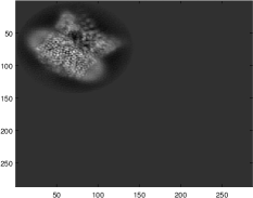
(b)

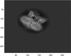
(c)

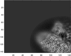
(d)

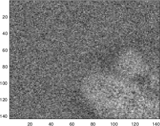
(e)

Figure 2: An illustration of the patch generation model described in (18).

Since in the E-step the algorithm assigns probabilities to rotations, the space of rotations must be discretized. We denote the set of $K$ discrete rotations by $\Omega^{K}\subseteq SO(3)$, such that $\omega_{p}\stackrel{{\scriptstyle\text{i.i.d.\ }}}{{\sim}}\operatorname{Unif}\left\{\Omega^{K}\right\}$; see Section IV for details. Higher $K$ provides higher accuracy at the cost of running time.

III-B EM iterations

III-B1 The E-step

Given a current estimate of the expansion coefficients $x_{k}$ and the distribution of translations $\rho_{k}$, in the E-step, our algorithm calculates the expected log-likelihood

$$Q\left(x,\rho|x_{k},\rho_{k}\right)=\mathbb{E}\left[\log\mathfrak{L}|\mathcal{I}_{1},\ldots,\mathcal{I}_{N_{\text{patches}}};x_{k},\rho_{k}\right],$$ (20)

where

$$\mathfrak{L}=\prod_{p=1}^{N_{\text{patches}}}p(\mathcal{I}_{p},\vec{\ell}_{p},\omega_{p};x,\rho),$$ (21)

which is a surrogate of the computationally intractable complete likelihood function. The expectation is taken over the possible translations and rotations, to achieve

$$Q(x,\rho|x_{k},\rho_{k})\\ =\sum_{p=1}^{N_{\text{patches}}}\sum_{\vec{\ell}\in\mathbb{L}}\sum_{\omega\in\Omega^{K}}p(\vec{\ell}_{p},\omega_{p}|\mathcal{I}_{p};x_{k},\rho_{k})\log p(\mathcal{I}_{p},\vec{\ell}_{p},\omega_{p}|x,\rho).$$ (22)

Applying Bayes’ rule, we have that

$$p(\vec{\ell}_{p},\omega_{p}|\mathcal{I}_{p};x_{k},\rho_{k})\\ =\frac{p(\mathcal{I}_{p}|\vec{\ell}_{p},\omega_{p};x_{k},\rho_{k})p(\vec{\ell}_{p},\omega_{p}|x_{k},\rho_{k})}{\sum_{\vec{\ell^{\prime}}\in\mathbb{L}}\sum_{\omega^{\prime}\in\Omega^{K}}p(\mathcal{I}_{p}|\vec{\ell^{\prime}},\omega^{\prime};x_{k},\rho_{k})p(\vec{\ell^{\prime}},\omega^{\prime}|x_{k},\rho_{k})},$$ (23)

which is just the normalized likelihood function

$$p(\mathcal{I}_{p}|\vec{\ell}_{p},\omega_{p};x_{k},\rho_{k})\propto\exp\left(-\frac{\|\mathcal{I}_{p}-CT_{\vec{\ell_{p}}}ZPR_{\omega_{p}}f\|_{\text{F}}^{2}}{2\sigma^{2}}\right),$$ (24)

with the normalization $\sum_{\vec{\ell}\in\mathbb{L}}\sum_{\omega\in\Omega^{K}}p(\mathcal{I}_{p}|\vec{\ell}_{p},\omega_{p};x_{k},\rho_{k})=1$, weighted by the prior distribution $p(\vec{\ell}_{p},\omega_{p}|x_{k},\rho_{k})=\frac{\rho_{k}[\vec{\ell}_{p}]}{K}$.

Thus, we can rewrite the expected log-likelihood function (22), up to a constant, as:

$$Q(x,\rho|x_{k},\rho_{k}) =\sum_{p=1}^{N_{\text{patches}}}\sum_{\vec{\ell}\in\mathbb{L}}\sum_{\omega\in\Omega^{K}}p(\mathcal{I}_{p}|\vec{\ell},\omega,x_{k})\rho_{k}[\vec{\ell}]$$

$$\times\left(\log p(\mathcal{I}_{p}|\vec{\ell},\omega,x)+\log\rho[\vec{\ell}]\right).$$ (25)

III-B2 The M-step

The M-step updates $x$ and $\rho$ by maximizing $Q(x,\rho|x_{k},\rho_{k})$ under the constraint that $\rho$ is a distribution function:

$$x_{k+1},\rho_{k+1}=\operatorname*{arg\,max}_{x,\rho}Q(x,\rho|x_{k},\rho_{k})\\ \text{ s.t. }\sum_{\vec{\ell}\in\mathbb{L}}\rho[\vec{\ell}]=1,\quad\rho[\vec{\ell}]\geq 0\text{ for }\vec{\ell}\in\mathbb{L}.$$ (26)

The constrained maximization of (26) can be achieved by maximizing the Lagrangian

$$\mathcal{L}(x,\rho,\lambda)=Q\left(x,\rho|x_{k},\rho_{k}\right)+\lambda\left(1-\sum_{\vec{\ell}\in\mathbb{L}}\rho[\vec{\ell}]\right),$$ (27)

where $\lambda$ is the Lagrange multiplier. As we will see next, the constraint of (17) is automatically satisfied at the maximum of the Lagrangian.

Algorithm 1 A stochastic approximate EM for cryo-EM

Input: measurement $\mathcal{I}$ partitioned to $N_{\text{patches}}$ patches; patch size $L$; parameter $K$ (number of discretized rotations); noise variance $\sigma^{2}$; initial guesses $x_{0}$ and $\rho_{0}$; stopping parameter $\epsilon$; maximal number of iterations $N_{\text{it}}$; stochastic factor $0<S\leq 1$.
Output: an estimate of $x$ and $\rho$.

  Set $k\rightarrow 0$;

  Set $\mathfrak{I}_{0;S}:\left\lfloor SN_{\text{patches}}\right\rfloor$ patches, drawn from a uniform distribution;

  Calculate $p(\mathfrak{I}_{0;S}|\vec{\ell},\omega;x_{0},\rho_{0})$ according to (24) for the set $\mathfrak{I}_{0;S}$, all $\omega\in\Omega^{K}$, and all $\vec{\ell}\in\mathbb{L}$;

  Calculate $Q_{0}$ according to (III-B1) for patches in $\mathfrak{I}_{0;S}$, and set $Q_{-1}\rightarrow-\infty$;

  while $\left(Q_{k}-Q_{k-1}\right)>\epsilon$ and $k<N_{\text{it}}$ do

     Update $x_{k+1}$ according to (29);

     Update $\rho_{k+1}$ according to (37);

     Set $\mathfrak{I}_{k+1;S}:\left\lfloor SN_{\text{patches}}\right\rfloor$ patches, drawn from a uniform distribution;

     Calculate $p(\mathfrak{I}_{k+1;S}|\vec{\ell},\omega;x_{k+1},\rho_{k+1})$ according to (24) for the set $\mathfrak{I}_{k+1;S}$, all $\omega\in\Omega^{K}$, and all $\vec{\ell}\in\mathbb{L}$;

     Calculate $Q_{k+1}$ according to (III-B1) for patches in $\mathfrak{I}_{k+1;S}$; Set $k\rightarrow k+1$;

  end while

  return   $x_{k},\rho_{k}$

Since $Q(x,\rho|x_{k},\rho_{k})$ is additively separable for $x$ and $\rho$, we maximize $\mathcal{L}(x,\rho,\lambda)$ with respect to $x$ and $\rho$ separately. At the maximum of $\mathcal{L}(x,\rho,\lambda)$, we have

$$0=\frac{\partial\mathcal{L}}{\partial{x_{\ell,m,s}}}\\ =\sum_{p=1}^{N_{\text{patches}}}\sum_{\vec{\ell}\in\mathbb{L}}\sum_{\omega\in\Omega^{K}}p(\mathcal{I}_{p}|\vec{\ell},\omega,x_{k})\rho_{k}[\vec{\ell}]\frac{\partial\log p(\mathcal{I}_{p}|\vec{\ell},\omega,x)}{\partial{x_{\ell,m,s}}},$$ (28)

resulting in a set of linear equations

$$y_{k}=A_{k}x_{k+1},$$ (29)

where $y_{k}$ is given by (III-B2) and $A_{k}$ is given by (III-B2), and $\odot$ is the Hadamard product. Notably, we can rewrite (III-B2) as (32), where $q(p,\vec{\ell},\omega;\ell,m,s)$ is given by (33). Furthermore, we can rewrite $A_{k}$ from (III-B2) as (34), where $g(\vec{\ell},\omega;\ell,m,s;\tilde{\ell},\tilde{m},\tilde{s})$ is given by (III-B2). The term $g$ is independent of the data $\left\{\mathcal{I}_{p}\right\}_{p=1}^{N_{\text{patches}}}$ and of the current estimate $x_{k}$, and thus can be precomputed once before the EM iterations; see Section III-E for a discussion about the computational complexity of the EM algorithm.

$$y_{k}\left[\ell,m,s\right] :=\sum_{p=1}^{N_{\text{patches}}}\sum_{\omega\in\Omega^{K}}\sum_{\vec{\ell}\in\mathbb{L}}p(\mathcal{I}_{p}|\vec{\ell},\omega,x_{k})\rho_{k}[\vec{\ell}]\sum_{N=-\ell}^{\ell}\sum_{n=0}^{n_{\text{max}}(N)}\widehat{\beta}_{\ell,s;N,n}D_{N,m}^{\ell}(\omega)$$

$$\times\sum_{i=0}^{L-1}\sum_{j=0}^{L-1}\mathcal{I}_{p}[i,j](Z\psi_{N,n})[(i+\ell_{x})\bmod 2L,(j+\ell_{y})\bmod 2L]$$ (30)

$$A_{k}\left[\ell,m,s;\tilde{\ell},\tilde{m},\tilde{s}\right] :=\sum_{p=1}^{N_{\text{patches}}}\sum_{\omega\in\Omega^{K}}\sum_{\vec{\ell}\in\mathbb{L}}p(\mathcal{I}_{p}|\vec{\ell},\omega,x_{k})\rho_{k}[\vec{\ell}]\sum_{\tilde{N}=-\tilde{\ell}}^{\tilde{\ell}}\sum_{\tilde{n}=0}^{n_{\text{max}}(\tilde{N})}\widehat{\beta}_{\tilde{\ell},\tilde{s};\tilde{N},\tilde{n}}D_{\tilde{N},\tilde{m}}^{\tilde{\ell}}(\omega)\sum_{N=-\ell}^{\ell}\sum_{n=0}^{n_{\text{max}}(N)}\widehat{\beta}_{\ell,s;N,n}D_{N,m}^{\ell}(\omega)$$

$$\times\sum_{i=0}^{L-1}\sum_{j=0}^{L-1}(Z\psi_{\tilde{N},\tilde{n}}\odot Z\psi_{N,n})[(i+\ell_{x})\bmod 2L,(j+\ell_{y})\bmod 2L]$$ (31)

$$y_{k}\left[\ell,m,s\right]=\sum_{p=1}^{N_{\text{patches}}}\sum_{\omega\in\Omega^{K}}\sum_{\vec{\ell}\in\mathbb{L}}p(\mathcal{I}_{p}|\vec{\ell},\omega,x_{k})\rho_{k}[\vec{\ell}]q(p,\vec{\ell},\omega;\ell,m,s)$$ (32)

$$q(p,\vec{\ell},\omega;\ell,m,s) :=\sum_{N=-\ell}^{\ell}\sum_{n=0}^{n_{\text{max}}(N)}\widehat{\beta}_{\ell,s;N,n}D_{N,m}^{\ell}(\omega)\sum_{i=0}^{L-1}\sum_{j=0}^{L-1}\mathcal{I}_{p}[i,j](Z\psi_{N,n})[(i+\ell_{x})\bmod 2L,(j+\ell_{y})\bmod 2L]$$ (33)

$$A_{k}\left[\ell,m,s;\tilde{\ell},\tilde{m},\tilde{s}\right]=\sum_{\omega\in\Omega^{K}}\sum_{\vec{\ell}\in\mathbb{L}}\left\{\sum_{p=1}^{N_{\text{patches}}}p(\mathcal{I}_{p}|\vec{\ell},\omega,x_{k})\right\}\rho_{k}[\vec{\ell}]g(\vec{\ell},\omega;\ell,m,s;\tilde{\ell},\tilde{m},\tilde{s})$$ (34)

$$g(\vec{\ell},\omega;\ell,m,s;\tilde{\ell},\tilde{m},\tilde{s}) :=\sum_{\tilde{N}=-\tilde{\ell}}^{\tilde{\ell}}\sum_{\tilde{n}=0}^{n_{\text{max}}(\tilde{N})}\widehat{\beta}_{\tilde{\ell},\tilde{s};\tilde{N},\tilde{n}}D_{\tilde{N},\tilde{m}}^{\tilde{\ell}}(\omega)\sum_{N=-\ell}^{\ell}\sum_{n=0}^{n_{\text{max}}(N)}\widehat{\beta}_{\ell,s;N,n}D_{N,m}^{\ell}(\omega)$$

$$\times\sum_{i=0}^{L-1}\sum_{j=0}^{L-1}(Z\psi_{\tilde{N},\tilde{n}}\odot Z\psi_{N,n})[(i+\ell_{x})\bmod 2L,(j+\ell_{y})\bmod 2L]$$ (35)

In order to update $\rho$, we maximize $\mathcal{L}(x,\rho,\lambda)$ with respect to $\rho$:

$$0=\frac{\partial\mathcal{L}}{\mathcal{\rho}[\vec{\ell}]}=\sum_{p=1}^{N_{\text{patches}}}\sum_{\omega\in\Omega^{K}}p(\mathcal{I}_{p}|\vec{\ell},\omega,x_{k})\rho_{k}[\vec{\ell}]\frac{1}{\rho[\vec{\ell}]}-\lambda,$$ (36)

for $\vec{\ell}\in\mathbb{L}$. We thus obtain the update rule for $\rho$ as

$$\rho[\vec{\ell}]=\frac{1}{\lambda}\sum_{p=1}^{N_{\text{patches}}}\sum_{\omega\in\Omega^{K}}p(\mathcal{I}_{p}|\vec{\ell},\omega,x_{k})\rho_{k}[\vec{\ell}],$$ (37)

and $\lambda=N_{\text{patches}}$ from the normalization (17).

III-C Stochastic approximate EM

In order to alleviate the computational burden of the approximate EM scheme (see Section III-E), we apply a stochastic variant. We focus on incremental EM, first introduced in [neal1998view]. At each iteration, the incremental EM algorithm applies the E-step to a minibatch of the observed data; the parameters of the problem are updated using the standard M-step. In particular, for the model (3), at each iteration, we choose $\left\lfloor SN_{\text{patches}}\right\rfloor$ patches drawn uniformly from the set of patches, where $0<S\leq 1$. We denote the set of $\left\lfloor SN_{\text{patches}}\right\rfloor$ patches by $\mathfrak{I}_{k;S}$, where $k$ is the iteration index. A small $S$ will result in faster and less memory consuming iterations, at the possible cost of additional iterations. In our numerical experiments in Section IV we set $S=0.05$.

The stochastic approximate EM algorithm is summarized in Algorithm 1.

III-D Frequency marching

As another means to reduce the computational complexity of our scheme, we adopt the frequency marching concept, previously applied to cryo-EM tasks [barnett2017rapid, scheres2012relion, lan2020multi]. We start our stochastic EM procedure (Algorithm 1) with a low target frequency (small $\ell_{\text{max}}$) estimate. When the algorithm is terminated, we use the low frequency estimate as an initial guess for the stochastic EM procedure with a higher target frequency, and continue to gradually increase the frequencies. This way the lion’s share of iterations is done over the low frequency estimates. This is crucial since the computational complexity of the algorithm strongly depends on the frequency $\ell_{\text{max}}$: see the next section.

III-E Complexity analysis

The computational complexity of the approximate EM algorithm depends mainly on the computational complexity of forming and solving the linear system of equations (29) at each iteration.

We start with analyzing the complexity of forming the matrix $A_{k}$ (III-B2). The computational complexity of computing a single entry of $p(\mathcal{I}_{p}|\vec{\ell},\omega,x_{k})$, given by (24), is $O\left(L^{2}\right)$. Recall that we have $N_{\text{patches}}=(N/L)^{2}$, $2L^{2}$ possible shifts, and $K$ discrete rotations. In addition, the summations over the indices $\ell$, $m$, $s$, $N$, $n$, $\tilde{\ell}$, $\tilde{m}$, $\tilde{s}$, $\tilde{N}$, and $\tilde{n}$ are of $O\left(\ell_{\text{max}}\right)$ operations each. Consequently, the total number of coefficients $x_{\ell,m,s}$ is $O\left(\ell_{\text{max}}^{3}\right)$, and the total number of matrix entries is $O\left(\ell_{\text{max}}^{6}\right)$. As such, the computational complexity of computing each entry of $A_{k}$ brute force is  $O\left(\frac{N^{2}}{L^{2}}KL^{2}\ell_{\text{max}}^{4}L^{2}\right)=O\left(N^{2}KL^{2}\ell_{\text{max}}^{4}\right)$, and the total complexity of computing the matrix is $O\left(N^{2}KL^{2}\ell_{\text{max}}^{10}\right)$. However, we recall that $p(\mathcal{I}_{p}|\vec{\ell},\omega,x_{k})$ can be computed once at the beginning of each iteration with complexity of $O\left(\frac{N^{2}}{L^{2}}KL^{2}L^{2}\right)=O\left(N^{2}KL^{2}\right)$. In addition, as was noted in (34), we can massively reduce the computational complexity by precomputing the function $g(\vec{\ell},\omega;\ell,m,s;\tilde{\ell},\tilde{m},\tilde{s})$ just once at the beginning of the algorithm with complexity of $O\left(\ell_{\text{max}}^{10}L^{4}K\right)$. That is, the total computational complexity of computing the matrix $A_{k}$ is

$$O\left(L^{4}K\ell_{\text{max}}^{10}+V\left(N^{2}KL^{2}+\frac{N^{2}}{L^{2}}L^{2}K\ell_{\text{max}}^{6}\right)\right)$$

$$=O\left(\ell_{L^{4}K\text{max}}^{10}+V\left(N^{2}KL^{2}+N^{2}K\ell_{\text{max}}^{6}\right)\right)$$

$$=O\left(L^{4}K\ell_{\text{max}}^{10}+VN^{2}K\left(L^{2}+\ell_{\text{max}}^{6}\right)\right),$$

where $V$ is the number of iterations. When computing $y_{k}$ (III-B2), as was the case for computing $A_{k}$, $p(\mathcal{I}_{p}|\vec{\ell},\omega,x_{k})$ is computed once at the beginning of each iteration with complexity of $O\left(N^{2}KL^{2}\right)$. Moreover, the multiplication between the patches $\left\{\mathcal{I}_{p}\right\}_{p=1}^{N_{\text{patches}}}$ and the shifted and padded PSWF eigenfunctions $\psi_{N,n}$, denoted as $q(p,\vec{\ell},\omega;\ell,m,s)$ (33), can be computed just once at the beginning of the algorithm with complexity $O\left(N^{2}L^{2}K\ell_{\text{max}}^{5}\right)$. All in all, the computational complexity of computing $y_{k}$ is $O\left(N^{2}L^{2}K\ell_{\text{max}}^{5}+VN^{2}K\left(L^{2}+\ell_{\text{max}}^{3}\right)\right)$. The computational complexity of solving the linear system of $O\left(\ell_{\text{max}}^{3}\right)$ equations (29) is of computational complexity of $O\left(\ell_{\text{max}}^{9}\right)$. As such, the total computational complexity of the approximate EM algorithm (Algorithm 1) is given by

$$O\Big{(}L^{4}\ell_{\text{max}}^{10}K+N^{2}L^{2}\ell_{\text{max}}^{5}K\\ +V\left(N^{2}L^{2}K+N^{2}\ell_{\text{max}}^{6}K+\ell_{\text{max}}^{9}\right)\Big{)}.$$

The computational complexity consists of precomputations that require $O\left(L^{4}\ell_{\text{max}}^{10}K+N^{2}L^{2}\ell_{\text{max}}^{5}K\right)$ operations, and from $O\left(N^{2}L^{2}K+N^{2}\ell_{\text{max}}^{6}K+\ell_{\text{max}}^{9}\right)$ calculations required per iteration. We note that since we aim to estimate small molecular structures, $L^{3}$ (the dimension of the volume), and $\ell_{\text{max}}$ (the maximum frequency in the expansion (6)) are expected to be rather small. However, $N^{2}$—the total number of pixels in all micrographs—is expected to grow as the SNR decreases. Therefore, we expect that the computational complexity of the approximate EM algorithm will be governed by $O\left(VN^{2}K\ell_{\text{max}}^{6}\right)$. Thus, the running time is linear in the number of pixels in the micrograph and the number of rotations considered by the EM framework. The latter presents an accuracy-running time trade-off [kreymer2022approximate]. Future work includes more sophisticated and hierarchical techniques to control the sampling of the space of rotations, akin to existing methods in cryo-EM software [scheres2012relion, punjani2017cryosparc]. The benefit of the frequency marching procedure (see Section III-D) is clear from our analysis—the computational complexity depends on $\ell_{\text{max}}^{6}$.

When using the stochastic variant of our approximate EM (see Algorithm 1), the computational complexity of the algorithm is $O\left(S\tilde{V}N^{2}K\ell_{\text{max}}^{6}\right)$, where $\tilde{V}$ is the number of iterations. The computational complexity scales linearly with the stochastic factor $0<S\leq 1$. However, the number of iterations $\tilde{V}$ is expected to increase as we process less patches per iteration.

IV Numerical results

In this section, we present numerical results for the stochastic approximate EM recovery algorithm described in Section III. The micrographs for the experiments were generated as follows. We sample rotation matrices from $SO(3)$ uniformly at random as described in [shoemake1992uniform]. Given a volume and a sampled rotation matrix, we generate projections of the volume corresponding to the rotation matrix using the ASPIRE software package [garrett_wright_2023_7510635]. The projections are then placed in the measurement one by one; for each added projection, it is verified that the separation condition (5) is not violated. The number of projections in the measurement, $T$, is determined by the required density $\gamma=T\frac{N^{2}}{\tilde{L}^{2}}$, where $\tilde{L}^{2}$ is the size of a projection within the micrograph. Ultimately, the micrograph is corrupted by i.i.d. Gaussian noise with zero mean and variance corresponding to the desired SNR.

We present reconstructions from micrographs generated in two different ways:

• In the first method, we generate the micrograph from volumes of the original size. Due to computational constraints, we downsample the micrograph by a factor of $\tilde{L}/L$, where $\tilde{L}^{3}$ is the original size of the volume, and $L^{2}$ is the required projection size for computations; we aim to estimate a downsampled volume of size $L^{3}$. Importantly, we assume that the downsampled target volumes are bandlimited (as assumed in Section II-A), but do not force it upon them. That is to say, the volume recovery error is bounded by this approximation error. This method imitates the procedure one will perform on experimental data sets.

• In the second method, we generate the micrograph from volumes downsampled to size $L^{3}$, expanded using the expansion (6) up to the maximal frequency. By that, we follow exactly our mathematical model of the micrograph generation (see Section II) and we expect this method to outperform the first (more realistic) method.

We follow the standard convention in the cryo-EM literature, and measure the accuracy of the reconstruction using the Fourier shell correlation (FSC) metric. The FSC is calculated by correlating the 3-D Fourier components of two volumes (the ground truth $f_{\text{true}}$ and the estimation $f_{\text{est}}$) and summing over spherical shells in Fourier space:

$$\text{FSC}(r)=\frac{\sum_{r_{i}\in S_{r}}\hat{f}_{\text{true}}(r_{i})\cdot\hat{f}^{*}_{\text{est}}(r_{i})}{\sqrt{\sum_{r_{i}\in S_{r}}\lvert\hat{f}_{\text{true}}(r_{i})|^{2}\sum_{r_{i}\in S_{r}}|\hat{f}_{\text{est}}(r_{i})|^{2}}},$$ (38)

where $S_{r}$ is the spherical shell of radius $r$. We use the $0.5$ resolution cutoff: the resolution is determined as the frequency where the FSC curve drops below 0.5.

A note about the SNR metric

In the first method mentioned above, the micrographs are downsampled. The downsampling improves the SNR since the spectra of the volumes decay faster than the spectrum of the noise. Therefore, in the following reported numerical results, while we report the SNR for reproducibility purposes, we present a representative image of a micrograph for proper visual evaluation of the SNR.

IV-A Volume reconstructions

We present reconstructions of four volumes. All reconstructions were achieved by applying the stochastic approximate EM algorithm (Algorithm 1) with stochastic factor of $S=0.05$ and $K=552$ discrete rotations. The algorithm was initialized from an initial guess of the size of the target volume, whose entries were drawn i.i.d. from a Gaussian distribution with mean 0 and variance 1. In all experiments, we used 4 micrographs of size $N^{2}=2992^{2}\text{ pixels}$, with $T=118374$ total projections. Each experiment consists of $N_{\text{patches}}=295936\text{ patches}$, where in each iteration we use $\left\lfloor SN_{\text{patches}}\right\rfloor=14796\text{ patches}$. The experiments were performed on a machine with 96 cores of Intel(R) Xeon(R) Gold 6252 CPU @ 2.10GHz with 1.51 TB of RAM, and took less than approximately 45 minutes per EM iteration with $\ell_{\text{max}}=6$, approximately 75 minutes per iteration with $\ell_{\text{max}}=8$, and approximately 5 hours per iteration with $\ell_{\text{max}}=10$. The molecular visualizations were produced using UCSF Chimera [pettersen2004ucsf].

IV-A1 The 3-D Shepp-Logan phantom [shepp1974fourier]

We consider the 3-D Shepp-Logan phantom of size $\tilde{L}^{3}=11^{3}\text{ voxels}$. Fig. 3(b) presents the estimation results from micrographs with $\operatorname{SNR}=3.5$. First, we use the first micrograph generation method, i.e., we simulate the micrographs with the true volume. A representative excerpt of the micrograph is presented in Fig. 3(a). We have conducted 7 EM iterations with $\ell_{\text{max}}=6$, 10 iterations with $\ell_{\text{max}}=8$, and 8 iterations with $\ell_{\text{max}}=10$. A visual comparison between the true and estimated volumes is presented in Fig. 3(b), and the FSC curve is given in Fig. 3(c). Next, we use a 3-D Shepp-Logan phantom of size $\tilde{L}^{3}=11^{3}\text{ voxels}$ expanded up to $\ell_{\text{max}}=10$ as our ground truth. The simulated micrographs are of the same $\operatorname{SNR}=3.5$. A representative excerpt of the micrograph is presented in Fig. 3(d). We have conducted 31 EM iterations with $\ell_{\text{max}}=6$, 19 iterations with $\ell_{\text{max}}=8$, and 18 iterations with $\ell_{\text{max}}=10$. A visual comparison between the true and estimated volumes is presented in Fig. 3(e), and the FSC curve is provided in Fig. 3(f).

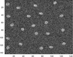
(a)

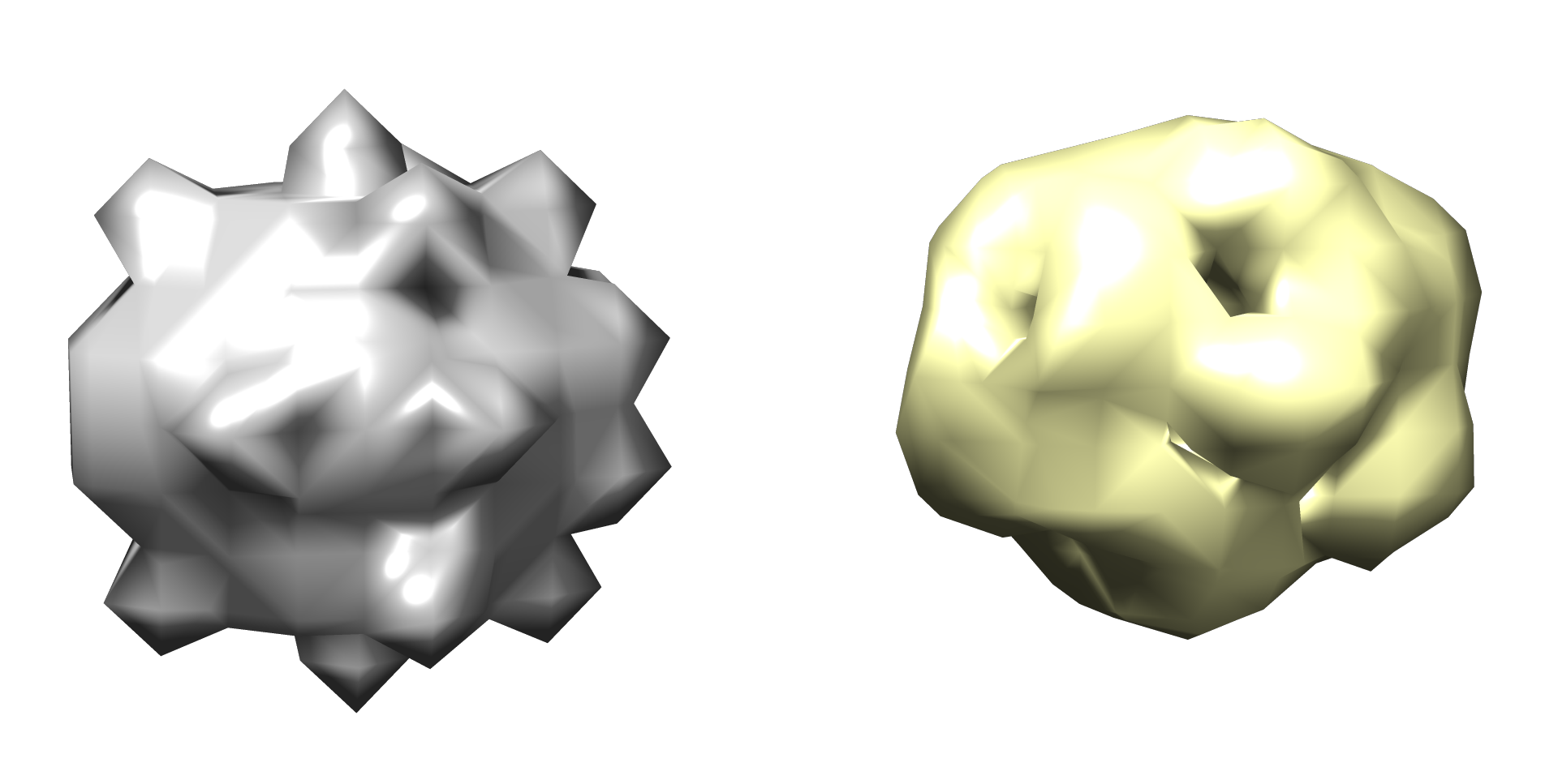
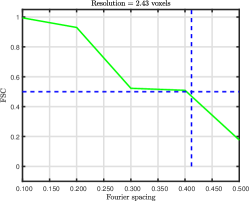
(b)

(c)

(d)

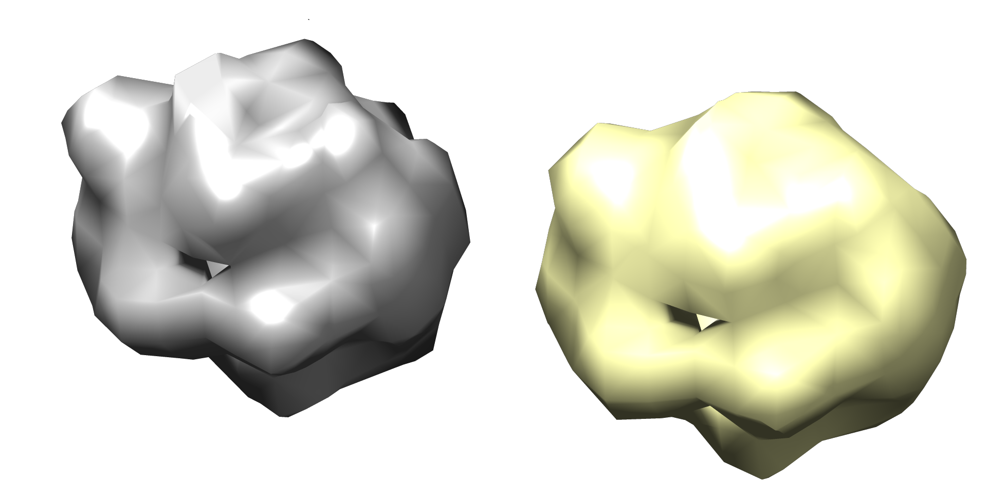
(e)

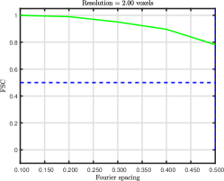
(f)

Figure 3: Results for estimating the 3-D Shepp-Logan phantom directly from a micrograph.

We can see, both visually and in terms of the FSC metric, that the estimation of the Shepp-Logan phantom is quite successful when we follow the mathematical model of Section II. However, when we aim to estimate the true, non-expanded, volume, the estimation is less accurate. This is since the true volume is not bandlimited, as is assumed in the expansion of Section II-A, so our expanded estimate fails to fully describe the true volume.

IV-A2 The TRPV1 structure [gao2016trpv1]

The volume is available at the Electron Microscopy Data Bank (EMDB) as EMD-8117. The true structure is of size $\tilde{L}^{3}=192^{3}\text{ voxels}$. We consider the downsampled version of the volume of size $L^{3}=11^{3}\text{ voxels}$. For this experiment, the micrographs were simulated with $\operatorname{SNR}=1$. We use the first micrograph generation method, i.e., we generate the micrographs with the true $192^{3}\text{ voxels}$ volume, and then downsample the micrographs such that each projection is of size $11\times 11\text{ pixels}$. A representative excerpt of the downsampled micrograph is presented in Fig. 4(a). We have conducted 14 EM iterations with $\ell_{\text{max}}=6$, 9 iterations with $\ell_{\text{max}}=10$, and 12 iterations with $\ell_{\text{max}}=10$. A visual comparison between the true and the estimated volumes is presented in Fig. 4(b), and the FSC curve is given in Fig. 4(c). Using the second micrograph generation method, we have generated the micrographs with $\operatorname{SNR}=3.5$. A representative excerpt of the micrograph is presented in Fig. 4(d). We have conducted 25 EM iterations with $\ell_{\text{max}}=6$, 8 iterations with $\ell_{\text{max}}=8$, and 4 iterations with $\ell_{\text{max}}=10$. A visual comparison is presented in Fig. 4(e), and the FSC curve is provided in Fig. 4(f).

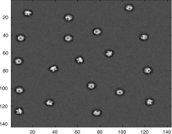
(a)

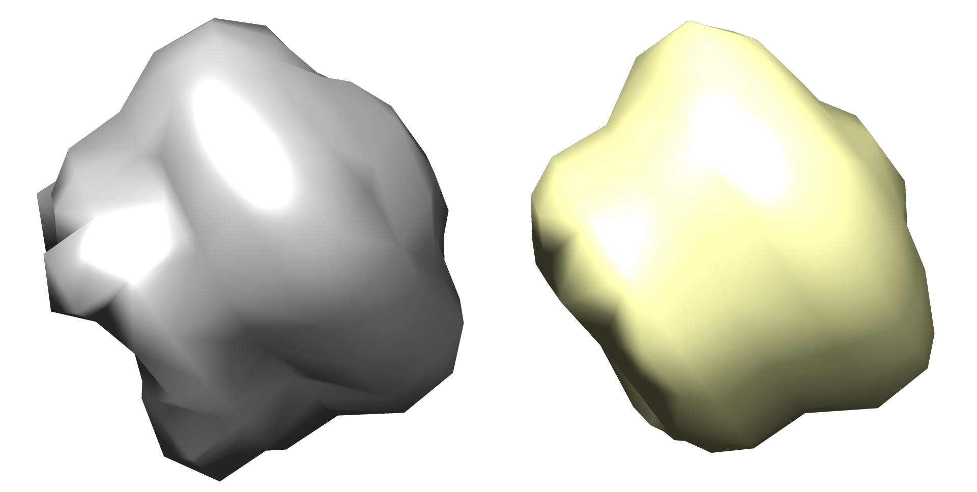
(b)

(c)

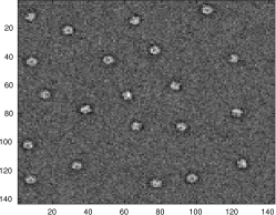
(d)

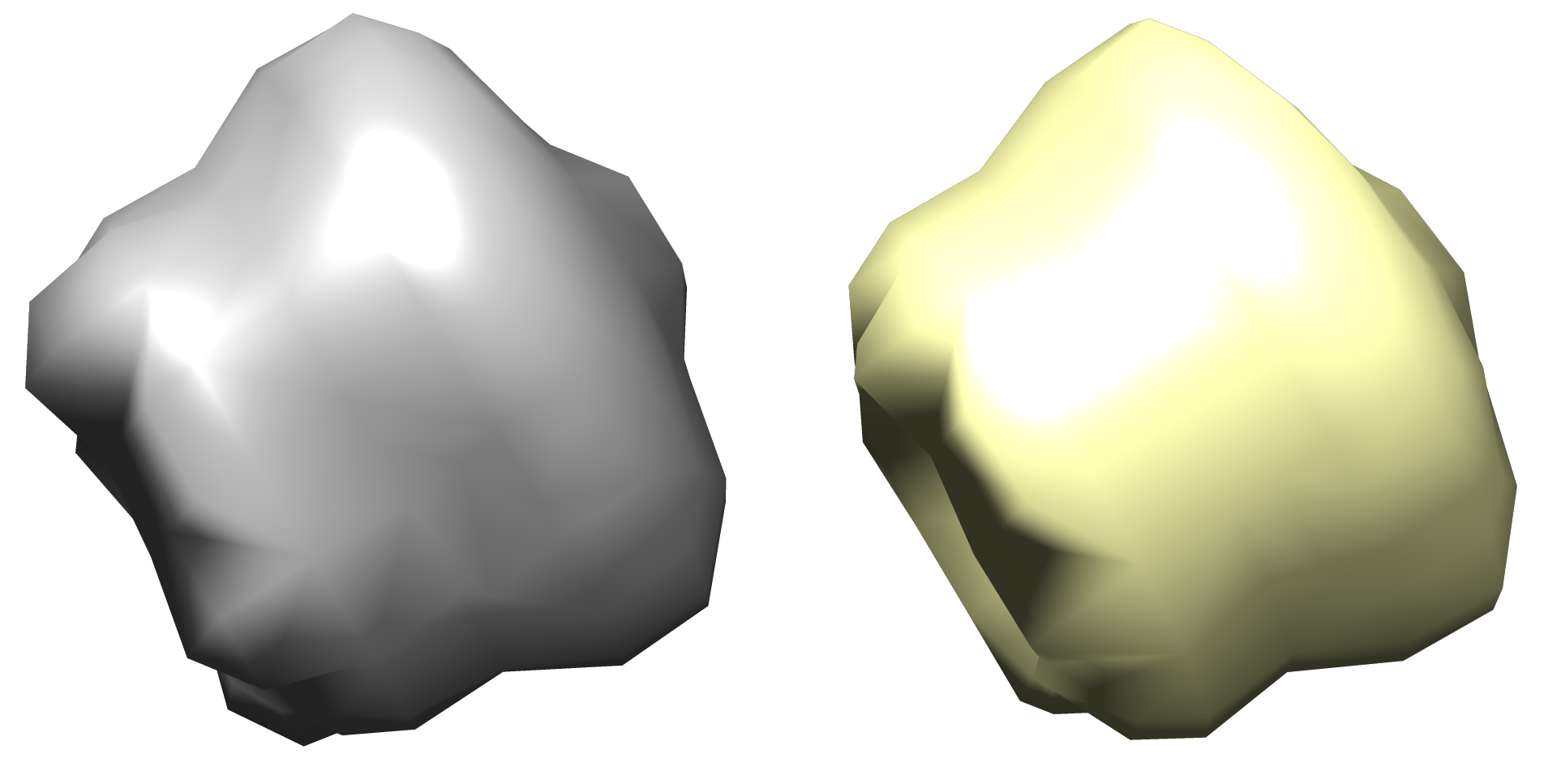
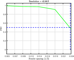
(e)

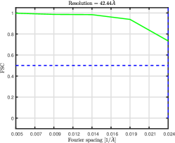
(f)

Figure 4: Results for estimating the TRPV1 structure directly from a micrograph.

Remarkably, we achieve accurate estimates of the downsampled TRPV1 structure from micrographs generated using both methods, perhaps due to its symmetrical structure. As expected, the result when we aim to estimate an expanded version of the volume is more accurate.

IV-A3 The Plasmodium falciparum 80S ribosome [wong2014cryo]

The volume is available at the EMDB as EMD-2660. The structure was cropped (to remove zeros at the boundaries) to size of $\tilde{L}^{3}=240^{3}\text{ voxels}$. First, we use the first micrograph generation method. For this experiment, the micrographs were simulated with $\operatorname{SNR}=1$. A representative excerpt of the downsampled micrograph is presented in Fig. 5(a). We have conducted 12 EM iterations with $\ell_{\text{max}}=6$, 16 iterations with $\ell_{\text{max}}=10$, and 8 iterations with $\ell_{\text{max}}=10$. A visual comparison between the true and the estimated volumes is presented in Fig. 5(b), and the FSC curve is given in Fig. 5(c). Next, we use a downsampled 80S ribosome of size $\tilde{L}^{3}=11^{3}\text{ voxels}$ expanded up to $\ell_{\text{max}}=10$ as our ground truth. The simulated micrographs are of $\operatorname{SNR}=3.5$. A representative excerpt of the micrograph is presented in Fig. 5(d). We have conducted 8 EM iterations with $\ell_{\text{max}}=6$, 8 iterations with $\ell_{\text{max}}=8$, and 13 iterations with $\ell_{\text{max}}=10$. A visual comparison between the true and the estimated volumes is provided in Fig. 5(e), and the FSC curve is presented in Fig. 5(f).

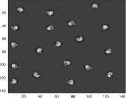
(a)

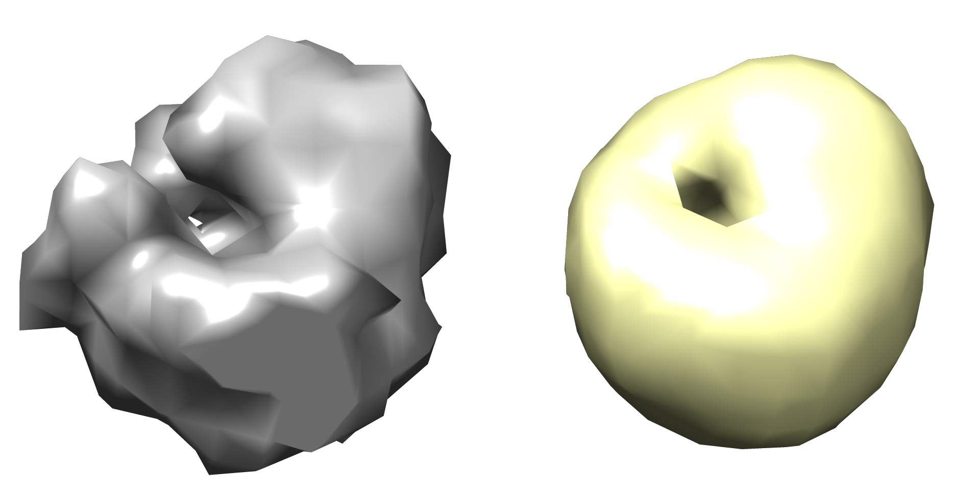
(b)

(c)

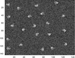
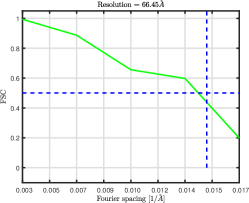
(d)

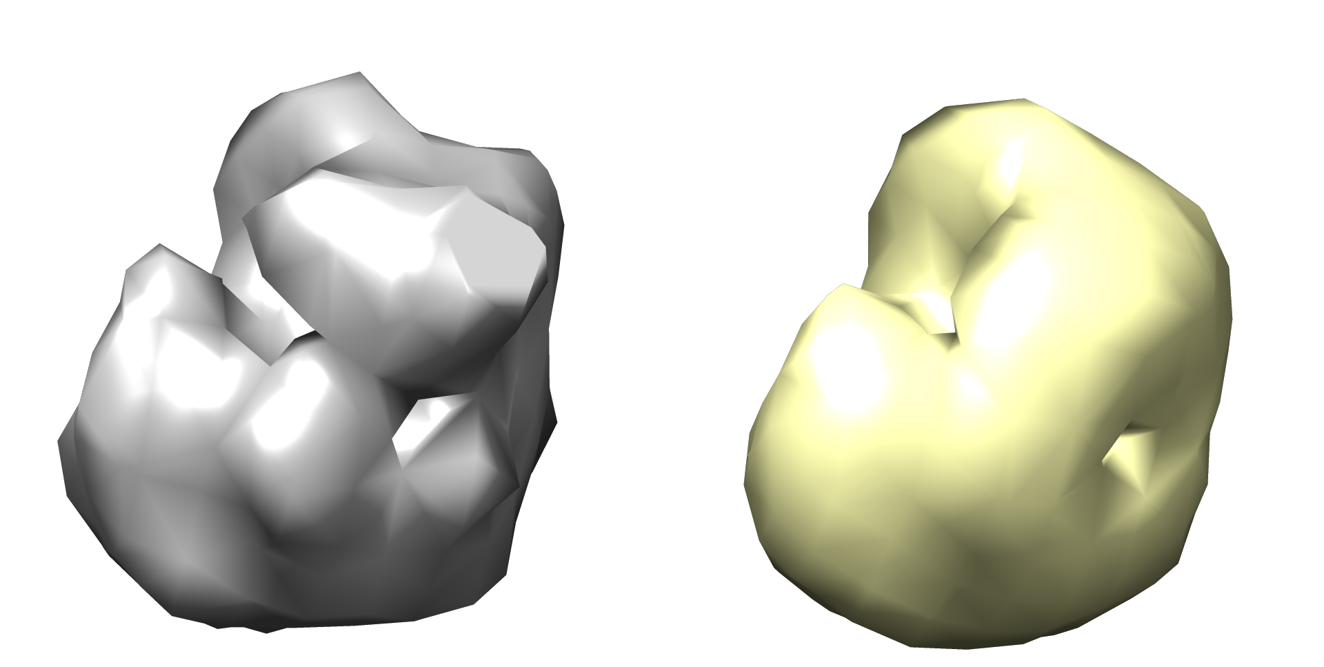
(e)

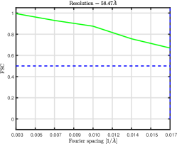
(f)

Figure 5: Results for estimating the Plasmodium falciparum 80S ribosome directly from a micrograph.

The estimation of the 80S ribosome is successful when we follow the mathematical model of Section II. However, when we aim to estimate the true, non-expanded, volume, the result is less accurate; the estimate follows the shape of the true downsampled volume, but the fine details are blurred. We believe that increasing the parameter $K$, the number of discrete rotations in the EM scheme, might improve the reconstruction accuracy, at the cost of running time (see Section III-E).

IV-A4 The Bovine Pancreatic Trypsin Inhibitor (BPTI) mutant [czapinska2000high]

The volume was generated in [bendory2023toward] from the atomic model from the Protein Data Bank (PDB), available as 1QLQ. The structure was cropped to size $\tilde{L}^{3}=31^{3}\text{ voxels}$. We consider the downsampled version of the volume of size $L^{3}=11^{3}\text{ voxels}$. First, we use the first micrograph generation method. For this experiment, the micrographs were simulated with $\operatorname{SNR}=0.75$. A representative excerpt of the downsampled micrograph is presented in Fig. 6(a). We have conducted 15 EM iterations with $\ell_{\text{max}}=6$, 10 iterations with $\ell_{\text{max}}=8$, and 9 iterations with $\ell_{\text{max}}=10$. A visual comparison between the true and the estimated volumes is presented in Fig. 6(b), and the FSC curve is given in Fig. 6(c). Next, we use a downsampled BPTI volume of size $\tilde{L}^{3}=11^{3}\text{ voxels}$ expanded up to $\ell_{\text{max}}=10$ as our ground truth. The simulated micrographs are of $\operatorname{SNR}=3.5$. A representative excerpt of the micrograph is presented in Fig. 6(d). We have conducted 22 EM iterations with $\ell_{\text{max}}=6$, 6 iterations with $\ell_{\text{max}}=8$, and 15 iterations with $\ell_{\text{max}}=10$. A visual comparison between the true and the estimated volumes is presented in Fig. 6(e), and the FSC curve is provided in Fig. 6(f).

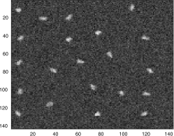
(a)

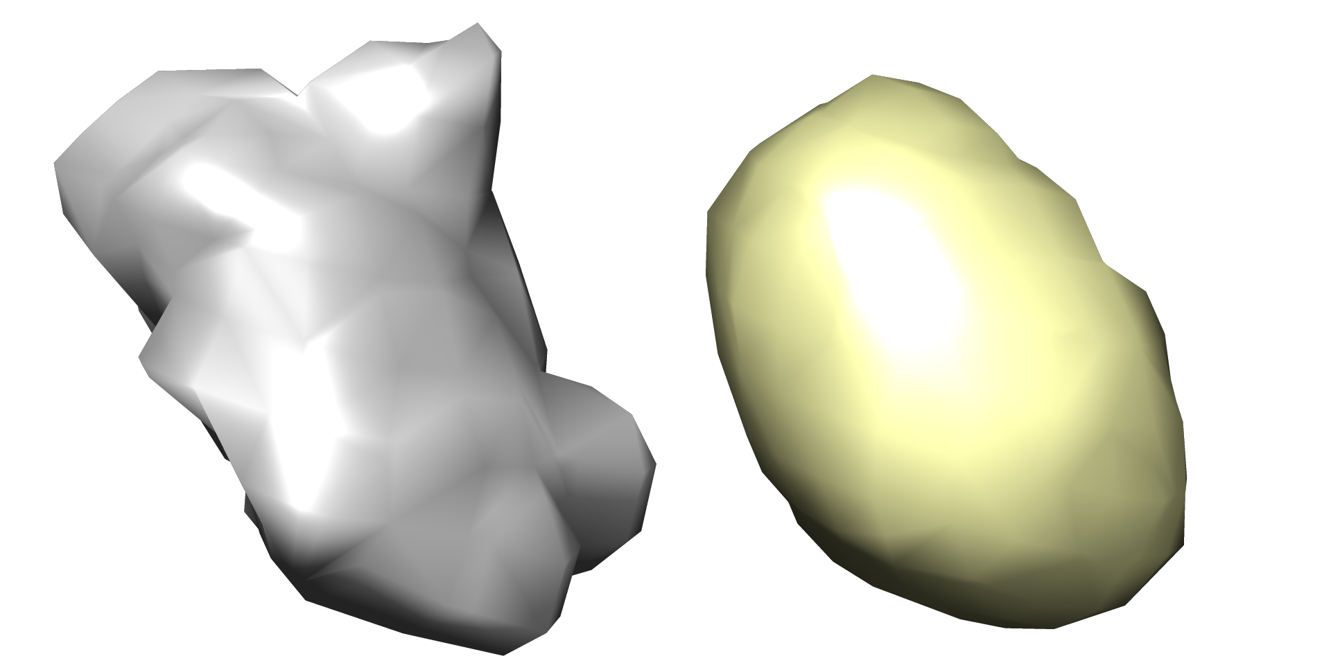
(b)

(c)

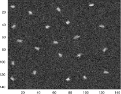
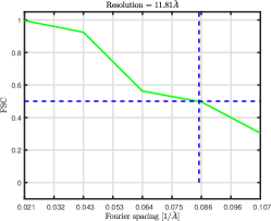
(d)

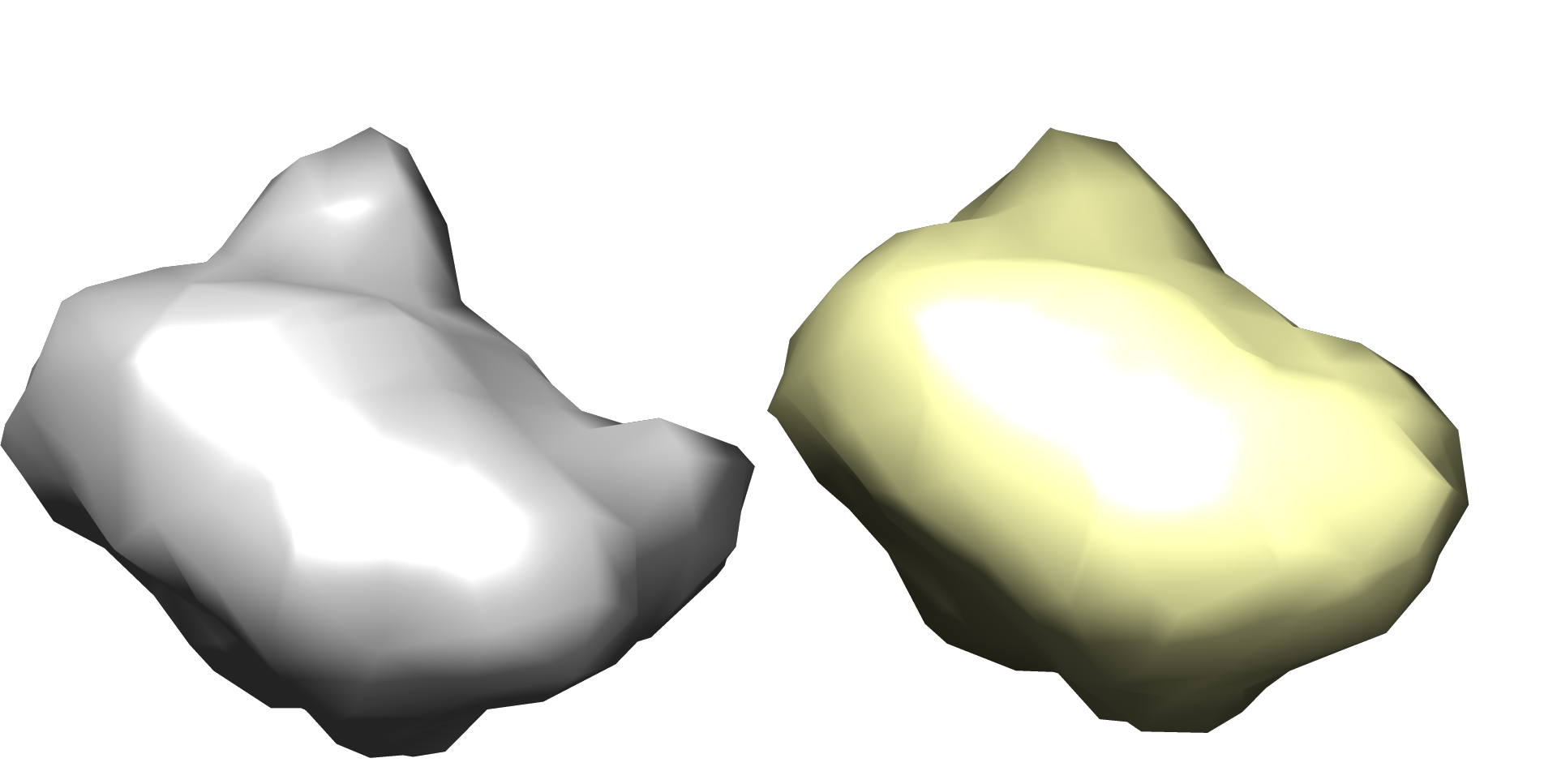
(e)

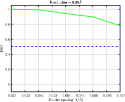
(f)

Figure 6: Results for estimating the Bovine Pancreatic Trypsin Inhibitor (BPTI) mutant directly from a micrograph.

We notice a similar phenomenon to the 80S ribosome estimation—the estimation of the BPTI mutant is successful when we follow the accurate mathematical model of Section II, and less accurate when we aim to estimate the non-expanded volume.

In comparison to the results of [bendory2023toward] using autocorrelation analysis, our results are of much higher frequency—$\ell_{\text{max}}=10$ versus $\ell_{\text{max}}=2$. In addition, the recovery in [bendory2023toward] is from clean autocorrelations, corresponding to $N\rightarrow\infty$, while our recoveries were done from noisy micrographs. We note that the reovery in [bendory2023toward] was done for a larger volume, of size $L^{3}=31^{3}\text{ voxels}$. Fig. 7 presents a visual comparison between our estimate and the downsampled estimate from [bendory2023toward].

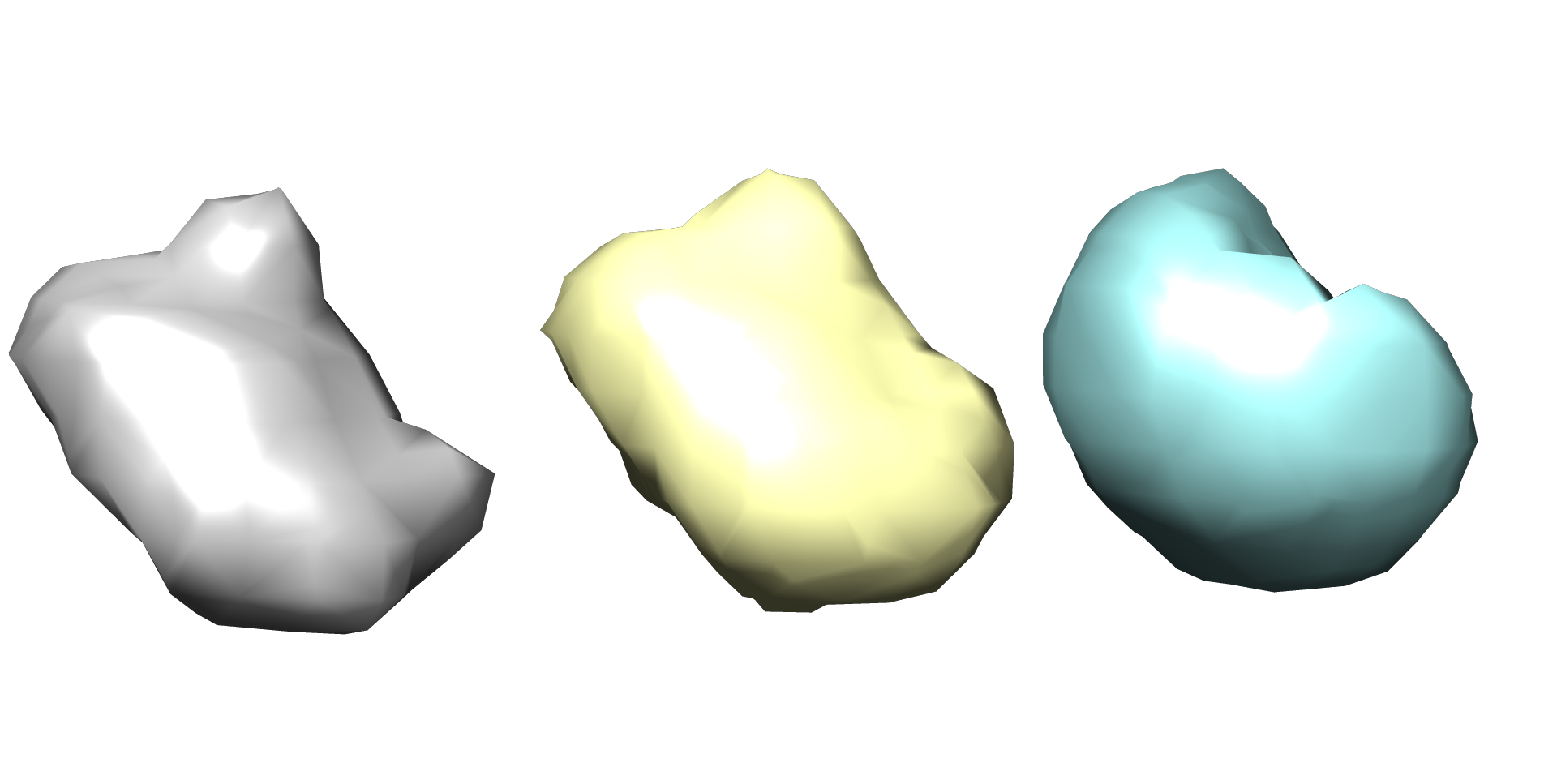
Figure 7: A visual comparison between the downsampled BPTI mutant (left), the estimate of the volume expanded up to $\ell_{\text{max}}=10$ using Algorithm 1 (middle), and the downsampled estimate of the volume using autocorrelation analysis, expanded up to $\ell_{\text{max}}=2$, as was estimated in [bendory2023toward] (right). The estimation in [bendory2023toward] was done from clean autocorrelations, corresponding to $N\rightarrow\infty$.

IV-B “Particle picking” using the approximate EM algorithm

During our EM procedure, we calculate the likelihood $p(\vec{\ell}_{p},\omega_{p}|\mathcal{I}_{p},x_{k})$ (see (23)) for each patch, where $x_{k}$ is the current estimate of the vector of coefficients. By averaging over the rotations, we get $p(\vec{\ell}_{p}|\mathcal{I}_{p},x_{k})$, which can be interpreted as the probability of each shift in the patch $\mathcal{I}_{p}$. Algorithm 2 introduces an algorithm to estimate the most probable shift in each patch. We stress that we do not suggest our algorithm as an alternative to existing particle pickers, but merely want to show that it succeeds to predict the true shifts if the SNR is high enough.

Algorithm 2 “Particle picking” using the approximate EM algorithm

Input: measurement $\mathcal{I}$ partitioned to $N_{\text{patches}}$ patches; patch size $L$; parameter $K$; noise variance $\sigma^{2}$; estimate $x$.
Output: the shifts $\left\{{\vec{\ell}_{{\text{picked}}_{p}}}\right\}_{p=1}^{N_{\text{patches}}}$, an estimate of the locations of particles within patches.

  Calculate $p\left(\vec{\ell}_{p},\omega_{p}|\mathcal{I}_{p},x\right)$ according to (23) for $p=1,\ldots,N_{\text{patches}}$;

  Calculate $p\left(\vec{\ell}_{p}|\mathcal{I}_{p},x\right):=\frac{1}{K}\sum_{\omega_{p}\in\Omega^{K}}p\left(\vec{\ell}_{p},\omega_{p}|\mathcal{I}_{p},x\right)$ for $p=1,\ldots,N_{\text{patches}}$;

  Calculate ${\vec{\ell}_{{\text{picked}}_{p}}}:=\operatorname*{arg\,max}_{\vec{\ell}_{p}\in\mathbb{L}}p\left(\vec{\ell}_{p}|\mathcal{I}_{p},x\right)$ for $p=1,\ldots,N_{\text{patches}}$;

  return   $\left\{{\vec{\ell}_{{\text{picked}}_{p}}}\right\}_{p=1}^{N_{\text{patches}}}$