SymX: Energy-based Simulation from Symbolic Expressions

Abstract.

Optimization time integrators have proven to be effective at solving complex multi-physics problems, such as deformation of solids with non-linear material models, contact with friction, strain limiting, etc. For challenging problems with high accuracy requirements, Newton-type optimizers are often used. This necessitates first- and second-order derivatives of the global non-linear objective function. Manually differentiating, implementing and optimizing the resulting code is extremely time-consuming, error-prone, and precludes quick changes to the model.

We present SymX, a framework based on symbolic expressions that computes the first and second derivatives by symbolic differentiation, generates efficient vectorized source code, compiles it on-the-fly, and performs the global assembly of element contributions in parallel. The user only has to provide the symbolic expression of an energy function for a single element in the discretization and our system will determine the assembled derivatives for the whole model. SymX is designed to be an integral part of a simulation system and can easily be integrated into existing ones. We demonstrate the versatility of our framework in various complex simulations showing different non-linear materials, higher-order finite elements, rigid body systems, adaptive cloth, frictional contact, and coupling multiple interacting physical systems. Moreover, we compare our method with alternative approaches and show that SymX is significantly faster than a current state-or-the-art framework (up to two orders of magnitude for a higher-order FEM simulation).

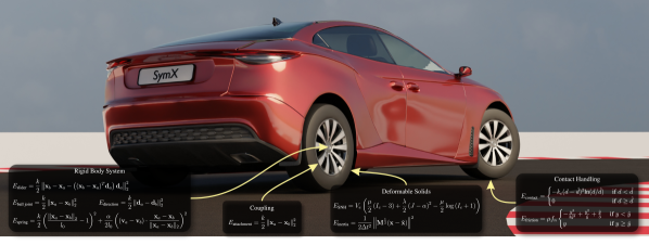
Figure 1. Simulation of a car drifting through a tight hairpin corner based on an optimization time integrator with strong coupling between rigid bodies and deformable solids. The simulation model consists of nine non-linear potential energies: linear FEM with the Stable Neo-Hookean model (Smith et al., 2018) for the tires, constraint-based energies (Macklin et al., 2020) for the rigid body components (sliders, ball joints, direction joints, and damped springs), and attachment constraints to couple the rigid body system for the suspension with the tires. Frictional contact potential is based on the Incremental Potential Contact method (Li et al., 2020). We are able to model complex simulations with SymX by virtue of succinctly defining the source energies using symbolic expressions and obtaining global derivatives that we use to solve the optimization time integration.

1. Introduction

In the research area of physically-based simulation a common problem is to efficiently compute the solution of non-linear equations, e.g., to simulate non-linear materials (Smith et al., 2018), to handle collisions with friction (Andrews et al., 2022), or to resolve non-linear constraints (Bender et al., 2014). This problem is also highly relevant for simulation methods based on energy minimization which have become increasingly popular in recent years (Gast et al., 2015; Narain et al., 2016; Brown et al., 2018; Chen et al., 2022). Such methods allow the user to combine different material models and constraints in a single simulation by formulating (typically non-linear) potential energy functions for each component. Implicit time integration is often performed by minimizing the sum of the inertia energy and all potential energies, e.g., using Newton’s method.

However, this minimization process typically requires the computation of the first and second derivatives of potentially very complex energy expressions which might even originate from different physical systems. Differentiating such energy expressions by hand can be hard and very time-consuming. Energies are often only defined locally for specific element types (e.g., tetrahedra). The global assembly of their derivatives in a system with different energy expressions and different element types can also be challenging if done by hand. Moreover, implementing and optimizing the code of complex expressions and their derivatives is error-prone and the software complexity increases as the number of physical systems and energies grow.

There already exist some tools which try to solve these problems, e.g., by computing the required derivatives using automatic differentiation. After analyzing several of these tools we defined requirements that such a tool should fulfill in the context of physically-based simulation:

• Automation: First and second derivatives should be computed and assembled completely automatically. In this way a researcher can focus on the energy function itself without caring about manually differentiating it or about an efficient implementation of the derivatives.

• Performance: The evaluation of the energy expression and its derivatives must be fast so that it can be directly used in a production system without further manual optimizations.

• Productivity: Fast iterations in a development process of a simulation system are desirable. Therefore, adding new energies or modifying expressions should be fast which requires a fast update of the derivatives and short compilation times of the resulting expressions.

• Flexibility: A tool should be easy to integrate in existing simulation systems and let the user choose their own data types and minimization solver. Moreover, an efficient handling of systems with changing sparsity patterns is required, e.g., to handle collisions that dynamically add energy terms, or to consider topology changes due to cutting, fracture, or spatial adaptivity.

In this paper we show in a detailed analysis that existing tools fail to fulfill at least one of these requirements. Based on these insights, we develop a new framework which computes the required derivatives by symbolic differentiation, generates efficient vectorized source code, compiles it on-the-fly, and provides an automatic assembly. This framework can easily be integrated in an existing simulation system and helps the user to quickly investigate and implement new energy functions in their system. We demonstrate the benefits of our method in various experiments where we simulate complex non-linear materials with higher-order finite elements, contact handling with friction, coupling of deformable solids and rigid bodies, and adaptive cloth models. For example, Fig. 1 shows a complex experiment, in which a car is simulated by combining multiple energy functions to simulate non-linear deformation of the tires, rigid-solid coupling of the rims and the tires, rigid bodies linked by different joint types, and contact with friction.

2. Related Work

In this section we first give an overview of simulation methods that require first and second-order derivatives to guarantee robustness. Then, we give an overview of the broad landscape of automated approaches to compute derivatives and cover other systems from the computer graphics literature that successfully made possible to express complex problems in terms of succinct expressions or programs while hiding complex optimizations from the user.

2.1. Optimization Time Integrators

Using an incremental potential formulation (Ortiz and Stainier, 1999) for dynamic problems is a common approach in computational mechanics. Derived or related methods also have become popular in computer animation where they are often referred to as optimization time integrators.

Formulating the dynamic systems as a scalar optimization problem instead of a non-linear system of equations was shown to be favorable for robustness and efficiency of the implementation (Kharevych et al., 2006; Gast et al., 2015). While this robustness is usually associated with Newton-style methods that use a full Hessian, local approaches such as Projective Dynamics (Bouaziz et al., 2014; Narain et al., 2016) can be used in case of stricter performance constraints. To still fulfill high accuracy requirements, Li et al. (2019) proposed a different method using domain decomposition that improves efficiency especially in case of extreme non-linear and high-speed deformations. While most of the previous works used an incremental potential formulation of backward Euler, Brown et al. (2018) presented a corresponding formulation of the TR-BDF2 integrator as part of a method to more accurately model dissipative forces.

Beside research to improve optimization-based methods in general, there is also widespread use of such methods for specific applications. This includes amongst others example-based elastic material simulation (Martin et al., 2011), where potentials guide deformations towards example data and crowd simulation which uses potentials to avoid collisions of agents (Karamouzas et al., 2017).

Recently, optimization-based contact models gained considerable popularity. The Incremental Potential Contact (IPC) approach (Li et al., 2020) and its extension to Codimensional IPC (Li et al., 2021) excel at providing robust interpenetration-free frictional contact handling. The characteristic robustness and convergence of such methods is subject to having access to second-order derivative information of the underlying global objective function. While contact potentials with barriers in general appear to be a promising choice for many applications, introducing them to orthogonal phenomenological research projects or existing multi-physics systems can require significant development effort. As we show later, our framework allows users to easily integrate models inspired by IPC into typical systems.

2.2. Differentiation

Automating the task of differentiation via computer programs has a long history, the dissertation of John F. Nolan (1953) being one of the original works in the field. Over the decades that followed, the relevancy of this field has seen huge leaps forward, and it is at the core of today’s most advanced technologies in important fields such as artificial intelligence. Since it is out of the scope of our work to give an extensive review of the field, we point the interested reader to the book by Griewank et al. (2008).

There are different strategies to differentiation. Automatic differentiation (AD) is perhaps the most widely used one due to its capabilities to handle derivatives of complex computer programs with dynamic control flow. In AD, a computation graph of the program to differentiate is built and derivative information is propagated along with the original computation. At a very high level, AD techniques can be divided in two main categories, backward and forward mode. The former one is more efficient when the program has a large number of degrees of freedom, while the latter can be more efficient otherwise. In recent years, the increased interest in machine learning has brought a lot of attention to backward AD techniques and very powerful tools, such as TensorFlow (Abadi et al., 2016) or PyTorch (Paszke et al., 2017), have been widely adopted. In our setting, however, thanks to the structure of the problem, we need to compute derivatives of local functions which depend on a relatively low number of degrees of freedom, therefore forward mode is usually preferred. We refer the reader to the work by Schmidt et al. (2022) which presents an in-depth discussion on the efficiency of forward and backward AD for such problems. The authors also provide an implementation, TinyAD, that is shown to outperform state-of-the-art tools in their applications.

On the other hand, Symbolic differentiation can be used to generate derivatives from input mathematical expressions. Dynamic loops and branching is usually more restricted in comparison to AD solutions, but the upside is that there is potentially more room for static analysis and optimization of the expressions, assuming that the target function can be described in closed form. Symbolic differentiation used as an external tool to the main application (e.g., using SymPy (Meurer et al., 2017) or Mathematica (Wolfram Research, 2023)) has seen some criticism (Schroeder, 2019) due lacking performance and the error-prone manual work that external tools introduce. However, efficiency concerns can be addressed by using Common Sub-expression Elimination (CSE) on the resulting derivative expressions, which can be carried out directly in the aforementioned tools. Recently, the work by Herholz et al. (2022) has proven that integrating symbolic differentiation in the application code, coupled with CSE and on-demand compilation can solve the performance shortcomings while making the process completely autonomous.

Further discussion on the relation between current differentiation approaches and our work is presented in Section 6.1.

2.3. Simulation Systems and DSLs

Alternative approaches include Domain Specific Languages (DSLs) to simplify the description and solution of specific problem classes or systems that process or encompass an entire simulation program. Liszt (DeVito et al., 2011) is a DSL designed to develop mesh-based PDE solvers that allows to define data at discretization nodes, batching subsequent operations for efficient processing. Simit (Kjolstad et al., 2016) and Ebb (Bernstein et al., 2016) are DSLs designed to ease writing high performance simulations by splitting the problem definition between data structures and simulation code and generating routines that avoid explicit sparse matrix assembly. More recently, Taichi (Hu et al., 2019) and MeshTaichi (Yu et al., 2022) take this further by allowing to switch internal data structures so the user has the possibility to find out which is the most suitable for their application.

Our method is an application specific approach, and as so there are other systems that are more closely related. DeVito et al. (2017) proposed a DSL to solve non-linear least squares problems with first-order methods from a concise objective function definition using symbolic differentiation at intermediate representation level. Further, Thallo (Mara et al., 2021) presents performance improvements by allowing computation and storage reorganization of the code.

Outside of DSLs, SANM (Jia, 2021) is a solver that applies the Asymptotic Numerical Method fully automatically to problems defined symbolically. ACORNS (Desai et al., 2022) generates first and second-order derivatives of target functions defined in the main application codebase at build time. Herholz et al. (2022) propose a code generator that transforms programs that symbolically define sparse operations into compiled high performance applications that avoid expensive sparse data structure bottlenecks. Similarly, Dr.Jit (Jakob et al., 2022) compiles per-scene kernels to accelerate execution times in the context of physically-based differentiable rendering. All three approaches employ either automatic or symbolic differentiation to internally generate derivatives from the user problem definition.

SymX follows the general philosophy of splitting core definitions (elemental energies and simulation discretization) from the internal procedures and data structures (evaluations and assembly), while also providing efficient differentiation facilities. To our knowledge, none of the aforementioned methods fulfill all of the requirements established in Section 1, some are too specialized to other applications, not flexible enough in terms of discretization and sparsity or in general not efficient enough especially considering second-order derivatives. However, we refer to Section 6.1 for an in-depth discussion about the feasibility of applying specific methods listed herein for our application.

3. Problem Definition

Many physical models used in simulation satisfy the following ordinary differential equation

(1) $$\boldsymbol{\mathbf{M}}\dot{\boldsymbol{\mathbf{v}}}=\boldsymbol{\mathbf{f}}(\boldsymbol{\mathbf{x}})=-\nabla E(\boldsymbol{\mathbf{x}}),\qquad\qquad\dot{\boldsymbol{\mathbf{x}}}=\boldsymbol{\mathbf{v}}.$$

Here $\boldsymbol{\mathbf{M}}$ is the mass matrix, $\boldsymbol{\mathbf{x}}$ is a vector containing some variant of positional degrees of freedom of the discrete system, $\boldsymbol{\mathbf{v}}$ similarly contains the velocity degrees of freedom, $\boldsymbol{\mathbf{f}}$ is a discrete representation of the forces acting on the system and $E$ is a scalar potential function. This ODE does not readily hold for rigid bodies without the introduction of a kinetic map (Bender et al., 2014), but in the interest of a simpler presentation we leave this aspect out of the present discussion. In general, dissipative forces like friction and damping do not have an associated scalar potential $E$, but it is often possible to work around this restriction by lagging the dissipative force in some fashion (Li et al., 2020).

To compute one time step of size $\Delta t$ for this problem, we may for example use the reformulation of Backward Euler as an optimization problem (cf. (Gast et al., 2015; Narain et al., 2016; Kugelstadt et al., 2018)) to obtain the incremental potential

(2) $$E_{\text{BE}}(\boldsymbol{\mathbf{x}}):=\frac{1}{2\Delta t^{2}}\left\|\boldsymbol{\mathbf{M}}^{\frac{1}{2}}(\boldsymbol{\mathbf{x}}-\tilde{\boldsymbol{\mathbf{x}}})\right\|^{2}+E(\boldsymbol{\mathbf{x}})=E_{\text{inertia}}(\boldsymbol{\mathbf{x}})+E(\boldsymbol{\mathbf{x}}),$$

where $\tilde{\boldsymbol{\mathbf{x}}}=\boldsymbol{\mathbf{x}}(t)+\Delta t\boldsymbol{\mathbf{v}}(t)+(\Delta t)^{2}\boldsymbol{\mathbf{M}}^{-1}\boldsymbol{\mathbf{f}}_{\text{ext}}$, $\boldsymbol{\mathbf{f}}_{\text{ext}}$ is the vector of constant external forces, and the associated update rules are

(3) $$\begin{split}\boldsymbol{\mathbf{x}}(t+\Delta t)&=\min_{\boldsymbol{\mathbf{x}}}E_{\text{BE}}(\boldsymbol{\mathbf{x}})\\ \boldsymbol{\mathbf{v}}(t+\Delta t)&=\frac{1}{\Delta t}\left(\boldsymbol{\mathbf{x}}(t+\Delta t)-\boldsymbol{\mathbf{x}}(t)\right).\end{split}$$

Other integrators will have a different formulation for the incremental potential and different update formulas, but in general we can describe the associated minimization problem as a sum of energy functions

(4) $$\min_{u}\sum_{i}E_{i}(\boldsymbol{\mathbf{u}};\mathcal{P}_{i})\,$$

in which we have used the state vector $\boldsymbol{\mathbf{u}}$ to describe the degrees of freedom, as for some applications it may favorable to pose the minimization problem either in terms of positional or velocity degrees of freedom. The abstract quantity $\mathcal{P}_{i}$ represents the parameters of the energy function $E_{i}$, i.e., the data of the problem that is not dependent on the state $\boldsymbol{\mathbf{u}}$.

Usually, energies can be decomposed into a number of smaller contributions. For example, the total strain energy $E_{\text{strain}}=\sum_{e}E_{\text{strain},e}$ for a deformable finite element model is the sum of the individual element strain energies $E_{\text{strain},e}$. To capture this inherent structure of the problem, we introduce abstract elements to the formulation. In practice, an element is an entity that has a contribution to the global potential energy, e.g., a tetrahedral finite element to simulate a deformable solid, a rigid body or a contact point between two objects. Each energy $E_{i}$ then gets associated with a set of elements $\mathcal{E}_{i}$ where it is defined and evaluated. We now replace Eq. (4) with our general problem formulation

(5) $$\min_{\boldsymbol{\mathbf{u}}}E(\boldsymbol{\mathbf{u}})=\sum_{i}\sum_{e\in\mathcal{E}_{i}}E_{i}(\boldsymbol{\mathbf{R}}_{e}\boldsymbol{\mathbf{u}};\mathcal{P}_{i,e})\,,$$

where $\boldsymbol{\mathbf{u}}$ denotes the global degrees of freedom and $\boldsymbol{\mathbf{R}}_{e}$ is the selection operator that extracts the degrees of freedom specific to the element $e$. $\mathcal{P}_{i,e}$ are the parameters specific to element $e$ for energy $i$. In other words, $\boldsymbol{\mathbf{R}}_{e}$ maps global to element-local quantities, and in consequence an energy $E_{i}$ operates only on element-local inputs of the same size. Its definition is independent of a specific element; only the parameters change.

Each energy function $E_{i}(\hat{\boldsymbol{\mathbf{u}}};\mathcal{P}_{i})$ is therefore a function of a generic vector $\hat{\boldsymbol{\mathbf{u}}}$ with fixed input size, evaluated for each associated element in $\mathcal{E}_{i}$. Since the number of distinct energy functions $E_{i}$ is typically a small constant, each associated with a particular discretization of some physical phenomenon, it is possible to symbolically represent, differentiate and generate code for each $E_{i}$, and finally assemble the final derivative of $E$ by summation.

Under the assumption that $E(\boldsymbol{\mathbf{u}})$ is at least $C^{1}$ continuous, we can efficiently solve (5) with an appropriate choice of optimizer (see (Nocedal and Wright, 2006)). First-order optimization methods require the gradient $\nabla E$, and second-order methods require the Hessian $\boldsymbol{\mathbf{H}}$ as well. For particularly challenging problems — such as those involving stiff materials or challenging contact — first-order methods may converge too slowly, and second-order methods are preferable, such as variants of Newton’s method. Although our method can be used with first-order methods, it is substantially more difficult to obtain efficient second-order derivatives, and therefore our framework brings even more to the table when used with second-order optimizers.

3.1. Example: Deformable solids

We now demonstrate how to formulate a motivating example within the mathematical framework of (5). We wish to simulate a deformable solid with the non-linear Neo-Hookean material using a linear tetrahedral finite element discretization and the Backward Euler integrator, subject to gravity. We let $\boldsymbol{\mathbf{u}}=\boldsymbol{\mathbf{x}}$ be the global vector of deformed vertex positions, and each element is associated with four vertices, forming a local vector $\hat{\boldsymbol{\mathbf{x}}}=\boldsymbol{\mathbf{R}}_{e}\boldsymbol{\mathbf{u}}=\boldsymbol{\mathbf{R}}_{e}\boldsymbol{\mathbf{x}}\in\mathbb{R}^{12}$ containing the deformed vertex positions stacked in an element-local vector. From this we can compute the deformation gradient $\boldsymbol{\mathbf{F}}_{e}=\boldsymbol{\mathbf{F}}_{e}(\hat{\boldsymbol{\mathbf{x}}})$ of the element (Sifakis and Barbic, 2012), which is constant across the element for the case of linear elements.

In general, the strain energy density $\psi=\psi(\boldsymbol{\mathbf{F}})$ for a hyperelastic material model depends only on the deformation gradient $\boldsymbol{\mathbf{F}}$. The strain energy density for the Neo-Hookean model is given by

(6) $$\psi^{\text{NH}}=\frac{\mu}{2}(I_{c}-3)+\mu\text{log}(\text{det}(\boldsymbol{\mathbf{F}}))+\frac{\lambda}{2}\text{log}^{2}\left(\text{det}(\boldsymbol{\mathbf{F}})\right),$$

where $\mu$ and $\lambda$ are the Lamé parameters and $I_{c}=\text{tr}(\boldsymbol{\mathbf{F}}^{T}\boldsymbol{\mathbf{F}})$ (Smith et al., 2018).

With the deformation gradient and strain energy density in hand, we can compute the strain energy for the element by integrating the strain energy density over its domain $K_{e}$, obtaining

(7) $$E_{\text{NH},e}(\hat{\boldsymbol{\mathbf{x}}})=\int_{K_{e}}\psi^{NH}(\boldsymbol{\mathbf{F}})\mathrm{d}\boldsymbol{\mathbf{X}}=V_{e}\,\psi^{NH}(\boldsymbol{\mathbf{F}}_{e}(\hat{\boldsymbol{\mathbf{x}}})).$$

Here $V_{e}$ denotes the volume of the element. We can formulate the inertia energy necessary for the Backward Euler incremental potential (2) in a similar fashion, and our total energy function for the minimization problem (5) becomes

(8) $$E(\boldsymbol{\mathbf{x}})=E_{\text{inertia}}+E_{\text{NH}}=\sum_{e}E_{\text{inertia},e}(\boldsymbol{\mathbf{R}}_{e}\boldsymbol{\mathbf{x}})+\sum_{e}E_{\text{NH},e}(\boldsymbol{\mathbf{R}}_{e}\boldsymbol{\mathbf{x}}).$$

Since the gradient and Hessian are computed by our framework, only the energy functions $E_{\text{inertia},e}$ and $E_{\text{NH},e}$ need to be provided in symbolic form by the user.

4. SymX Framework

We give a general overview of the framework in Section 4.1. The symbolic engine which is the core component of our framework is introduced in Secion 4.2. Finally, we discuss the required matrix assembly in Section 4.3. While we use a specific application example in this section to explain the components of our framework in detail, it is not limited to this use case and more complex applications are discussed in Section 5.

4.1. Overview

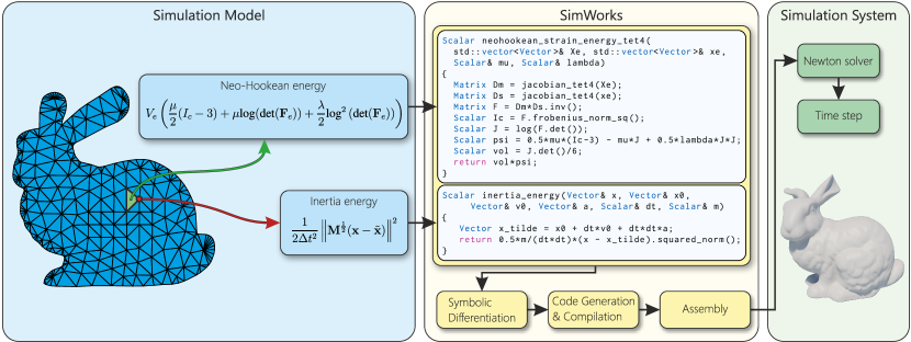
Figure 2. Overview of a simulation step with the SymX framework. Left: The input is a discretized model and energy functions. In our application example we use a tet mesh and the inertia and Neo-Hookean strain energy functions. Center: The user has to implement a symbolic definition of these functions. The framework will then compute the element gradients and Hessians by symbolic differentiation, generate and compile efficient code, and assemble the element contributions to get the full gradient and Hessians. Finally, these terms can be used in a Newton solver to perform a simulation step for the deformable bunny.

Computing and implementing first- and second-order derivatives needed for effective optimization manually can be time-consuming and error-prone. Our SymX framework solves this problem and provides an efficient method to compute the gradients and Hessians for all energy functions in a simulation. It can be directly integrated in an existing simulation system and there replaces the gradient and Hessian computation required for the minimization process.

Fig. 2 shows how the minimization problem of the deformable solids example in Section 3.1 is solved using our framework. For the simulation model on the left, the user has to implement mathematical expressions (center). Then our framework generates an expression graph and determines the derivatives using symbolic differentiation. For an efficient evaluation of an expression and, as required, its first and second derivative, SymX generates vectorized code, compiles it on-the-fly, and performs an automatic assembly of the resulting matrices in parallel. Finally, the user can combine several expressions that should be minimized and link their simulation data and connectivity information with the symbols used in the expressions (see Fig. 3). This enables our framework to autonomously loop over all elements, gather the data, evaluate the compiled expressions, and assemble the results.

In the following subsections we will explain the individual steps for our application example in more detail.

Figure 3. Map the simulation data and connectivity information (lines 2-6) to symbolic arrays (lines 10-17) to compute the Neo-Hookean strain energy for all tets (line 20) and the inertia energy for all nodes (line 33) as defined in our application example.

4.2. Symbolic Engine

The core of the SymX framework is our symbolic engine. As input the engine requires a symbolic mathematical expression for each energy of the minimization problem (5). The implementation of such an expression is straightforward. The only difference to a typical C++ implementation is that instead of using numerical standard types such as double or float, our symbolic types Scalar, Vector and Matrix must be used. The framework provides functionality like operator overloading and common linear algebra for these types. Fig. 2 shows the symbolic expressions of the Neo-Hookean potential energy and the inertia energy for the application example described in Section 3.1.

Instead of directly executing the instructions of a symbolic expression, our engine generates an expression graph. In this graph each node represents either a user-defined symbol, a constant value or an operation applied to the result of its child nodes. So far SymX supports arithmetic and trigonometric operations, square roots and logarithms. Conditional branching is a special type of operation that is discussed in Section 4.2.4.

In the following we describe the components of our symbolic engine step by step using the example of Section 3.1. However, keep in mind that our framework can also handle far more complex configurations (e.g., coupling multiple materials, using higher-order elements, handling collisions etc.) as we will show in Section 5.

4.2.1. Symbolic Differentiation

In the first step our framework computes the derivatives of the mathematical expressions by symbolic differentiation. A derivative with respect to a symbol is determined by traversing the expression graph recursively and applying derivative table look ups.

The expression graphs of the gradient and the Hessian typically often contain the same operations for different matrix entries. Evaluating such duplicate expressions can become a significant performance problem. Therefore, we use the expression compression technique of Herholz et al. (2022). In this way each expression is only evaluated once and duplicate entries use a cached result. In our example the expression complexity of the Hessian of the Neo-Hookean energy expression (see Fig. 2) was reduced by ~75%, from 7517 to 1873 operations.

4.2.2. Code Generation and Compilation

Once we have the expressions for a function and its derivatives, we need to evaluate them for the elements. To perform the evaluation efficiently we first traverse the expression graph and generate C++ code containing all operations. The generated C++ function operates as a black box, reading from an array of inputs and writing to an array of outputs. For example, the C++ function to evaluate the value, gradient and Hessian of the Neo-Hookean energy defined in Fig. 2 with respect to the vertices of a tet in the deformed configuration $\boldsymbol{\mathbf{x}}^{e}$ has 26 inputs (12 for $\boldsymbol{\mathbf{X}}^{e}$, 12 for $\boldsymbol{\mathbf{x}}^{e}$ and two for $\mu$ and $\lambda$) and 157 outputs (1 for the energy value, 12 for the gradient and 144 for the Hessian). After generating the C++ code, it is compiled on-the-fly (using standard compiler optimizations) at the beginning of the simulation and loaded as a binary shared object.

4.2.3. Data Mapping

To evaluate a compiled function we first need to determine the correct indices for all inputs and outputs which correspond to a set of selected degrees of freedom and element parameters (cf. Eq. (5)). Since the number of indices can be large (see above), a manual implementation can be time-consuming and error-prone. Therefore, we introduced the types Array and ConnectivityArray in our framework which allow a mapping of simulation data (e.g., positions, velocities, …) and connectivity information (e.g., tetrahedra, triangles, edges, …) to their corresponding symbolic representation, respectively. In this way the indexing of inputs and outputs can be handled automatically by the framework.

An example is shown in Fig. 3, where in lines 10-15 the data is mapped and in lines 16-17 the connectivity. Arrays which represent the degrees of freedom for the minimization must be defined in a special way (line 10) so that the framework knows that it should compute the derivatives with respect to these symbols. Scalar parameters can be defined directly from variables (lines 26, 27, 41, 42). In lines 20 and 33 we can then simply define energy functions for all tets and nodes, respectively, and our system will resolve all indices. Note that our framework keeps track of changes in the simulation data arrays so it can easily handle topology changes of the problem, e.g., due to dynamic collision response or adaptive mesh refinement.

4.2.4. Extensions

In the following we introduce extensions which are required for more complex simulations or to improve the performance of the system.

Branching

SymX supports differentiation and code generation of expressions with arbitrary nested branching using the command

where $c$ is a conditional variable, the expression $a$ is used if $c\geq 0$, and $b$ is used if $c<0$. In this way it is possible to implement energies with functions like min, max, abs and sign. In our experiments we use branching, for example, to implement the signed distance function of a capped cylinder. This function is used for collision detection (see Fig. 1). Note that since it has 47 branching points once it is unrolled, it is tedious to differentiate it manually and even if the code of the derivatives is generated automatically by a tool, the integration of the code is hard. The implementation and integration in a simulation using our framework was simple and just took a few minutes.

Conditional evaluations

A common use case in simulation is branching where the value of the second branch is zero, e.g., when modeling contact using inequality constraints. In this case the energy function is defined in combination with an activation condition:

(9) $$e=\sum_{e\in\mathcal{E}}e_{e},\;\;\;e_{e}=\begin{cases}e_{e}^{+}\,&\text{if}\,c_{e}>0\\ 0\,&\text{if}\,c_{e}\leq 0,\end{cases}$$

where $e_{e}^{+}$ is the energy of element $e$ and $c_{e}$ is its activation function. To handle such expressions efficiently, SymX also compiles the activation function and uses it to gather all active elements for the evaluation. In this way we can avoid the evaluation and assembly of zero energy terms and the corresponding derivatives.

Fixed value summations

In numerical simulation it is common to have an inner loop per element over a set of constant data. For example in FEM simulations we have to evaluate an energy density function multiplied with integration weights at a set of fixed integration points. In general, we can formulate this abstractly as the energy function

(10) $$E=\sum_{e\in\mathcal{E}}\sum_{k}\tilde{E}(\boldsymbol{\mathbf{R}}_{e}\boldsymbol{\mathbf{u}};\mathcal{P}_{e},\mathcal{P}_{k})$$

for some energy contribution $\tilde{E}$, where $\mathcal{P}_{k}$ are the parameters specific to the inner iteration $k$. In the example with integration points, $\mathcal{P}_{k}$ includes the $k$-th quadrature weight and point.

While it is possible to handle such energies by adding each iteration of the loop to the expression graph, this approach becomes expensive for complex expressions and even for moderate iteration counts. To solve this problem SymX compiles a single function for a symbolic set of inner iteration parameters and call the function multiple times with updated inputs. This approach scales very well to complex models and discretizations so that SymX is well-suited for higher-order FEM simulations as we demonstrate in Section 5.2.

Caching compiled functions

The symbolic differentiation, code generation and compilation typically takes less than one second for most expressions. However, in case of complex expressions or simulations with many different energies, recompiling all expressions can slow down the development process significantly. Therefore, SymX only differentiates and compiles new expressions or modified ones. This is implemented by computing an SHA256 hash for each expression and storing it in the compiled object. This feature enables fast iterations in the development process of complex simulation systems.

Parallelization and vectorization

To accelerate the evaluation of the expressions we parallelize the loop over all elements using OpenMP. Furthermore, vectorization is used internally in the framework to evaluate multiple elements per compiled function call at the same time.

4.3. Assembly

In our application example we only have one set of degrees of freedom. However, in this section we want to describe the assembly for the more general case of having multiple sets of degrees of freedom $\boldsymbol{\mathbf{u}}_{0},\dots\boldsymbol{\mathbf{u}}_{n}$, e.g., one set for deformable solids, one for cloth models, and one for the rigid body system. Example simulations are shown in Section 5.

In SymX, all sets are concatenated into a global vector $\boldsymbol{\mathbf{u}}$. This concatenation establishes a global indexing of the degrees of freedom, which is automatically considered by SymX during the assembly step. The linear system associated with a Newton iteration then takes the form

(11) $$\begin{pmatrix}\frac{\partial^{2}E}{\partial\boldsymbol{\mathbf{u}}_{1}^{2}}&\frac{\partial^{2}E}{\partial\boldsymbol{\mathbf{u}}_{1}\partial\boldsymbol{\mathbf{u}}_{2}}&\dots&\frac{\partial^{2}E}{\partial\boldsymbol{\mathbf{u}}_{1}\partial\boldsymbol{\mathbf{u}}_{n}}\\ \frac{\partial^{2}E}{\partial\boldsymbol{\mathbf{u}}_{2}\partial\boldsymbol{\mathbf{u}}_{1}}&\frac{\partial^{2}E}{\partial\boldsymbol{\mathbf{u}}_{2}^{2}}&\dots&\frac{\partial^{2}E}{\partial\boldsymbol{\mathbf{u}}_{2}\partial\boldsymbol{\mathbf{u}}_{n}}\\ \vdots&\vdots&\ddots&\vdots\\ \frac{\partial^{2}E}{\partial\boldsymbol{\mathbf{u}}_{n}\partial\boldsymbol{\mathbf{u}}_{1}}&\frac{\partial^{2}E}{\partial\boldsymbol{\mathbf{u}}_{n}\partial\boldsymbol{\mathbf{u}}_{2}}&\dots&\frac{\partial^{2}E}{\partial\boldsymbol{\mathbf{u}}_{n}^{2}}\\ \end{pmatrix}\cdot\begin{pmatrix}\Delta\boldsymbol{\mathbf{u}}_{1}\\ \Delta\boldsymbol{\mathbf{u}}_{2}\\ \vdots\\ \Delta\boldsymbol{\mathbf{u}}_{n}\\ \end{pmatrix}=-\begin{pmatrix}\frac{\partial E}{\partial\boldsymbol{\mathbf{u}}_{1}}\\ \frac{\partial E}{\partial\boldsymbol{\mathbf{u}}_{2}}\\ \vdots\\ \frac{\partial E}{\partial\boldsymbol{\mathbf{u}}_{n}}\end{pmatrix},$$

where $E$ is the global energy of the simulation. The diagonal blocks in the global Hessian matrix contain the second derivatives of internal energies to a physical system, such as strain energies for deformable objects, while off-diagonal blocks contain the second derivatives of inter-system interactions, such as collisions or attachments.

SymX has a default custom concurrent data structure to build and return the global Hessian and the gradient. This data structure is based on the Blocked Compressed Row Storage (BCRS) sparse matrix format. However, our framework can also return the local gradients and Hessians of the elements together with the global indices. In this way existing simulation systems can easily use their own data structures.

5. Applications

In the previous section we introduced our framework for a typical application example in the area of physically-based animation. However, SymX is not limited to this specific problem. Therefore, in the following we show how complex problems in the area of physically-based simulation can be solved using our framework.

5.1. Non-Linear Material Models

In a simulation system it is often desirable to implement different material models with different properties. To demonstrate that it is easy for a user to extend their simulator by new materials when using SymX, we implemented five different material models in an experiment: the As-Rigid-As-Possible (ARAP) model as described by Lin et al. (2022), the fixed co-rotational by Stomakhin et al. (2012), St. Venanant-Kirchhoff (StVK), and both Neo-Hookean and Stable Neo-Hookean models as described by Smith et al. (2018). The last material is the most complex one. However, its implementation in SymX is straightforward, took only a few minutes, and just requires a few lines of code:

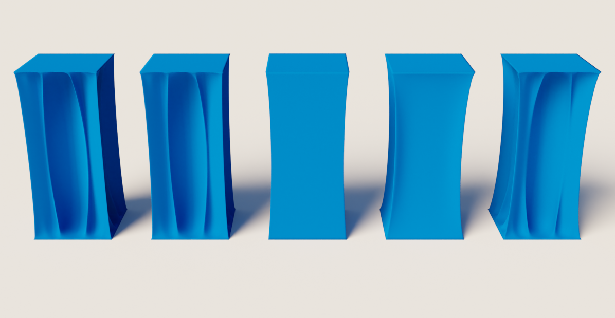
Figure 4. Comparison of different material models in a simulation of a stretched deformable cube. From left to right: As-Rigid-As-Possible, fixed co-rotational, St. Venant-Kirchhoff (StVK), Neo-Hookean and Stable Neo-Hookean material.

The code for all the materials method can be found in Appendix A. Figure 4 shows a comparison of the materials in a simulation of a stretched cube. The result shows the characteristic deformation behavior of the material models, which is comparable to the results of Smith et al. (2018). Note that a manual implementation of the material energy, its derivatives, and the assembly is far more complex than the code shown above.

5.2. Higher-Order Finite Elements

In our application example we used a linear FEM discretization to illustrate how our pipeline works. However, SymX is not tied to any particular discretization and can also be used in higher-order FEM simulations. For higher-order elements, numerical integration rules are often used, so that the total deformation energy of an element is given by

(12) $$E_{e}^{FEM}=\sum_{i=1}^{p}w_{i}\,\det(\boldsymbol{\mathbf{J}}^{e}_{0})\,\psi\left(\boldsymbol{\mathbf{F}}(\boldsymbol{\mathbf{\xi}}_{i},\boldsymbol{\mathbf{X}}^{e},\boldsymbol{\mathbf{x}}^{e})\right),$$

where $\psi$ is the strain energy density function, $p$ is the number of integration points, and $w_{i}$ represents the quadrature weight. The integration point $\boldsymbol{\mathbf{\xi}}_{i}$ is defined in the coordinate system of the reference element, and $\boldsymbol{\mathbf{J}}^{e}_{0}=\boldsymbol{\mathbf{J}}^{e}_{0}(\boldsymbol{\mathbf{\xi}}_{i})$ is the Jacobian of the mapping from the reference element to the physical element in the undeformed configuration (see, e.g., Wriggers et al. (2008)).

For brevity we assume in the following code that the functions jac and psi are already defined to compute the Jacobian for an element and the strain energy density, respectively. Then the following code shows the implementation of Eq. (12) in SymX:

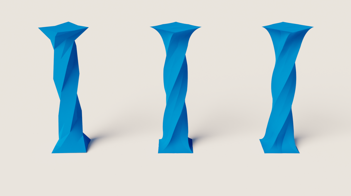
Figure 5. Comparison of linear (left), quadratic (center) and cubic (right) finite elements in a simulation of a stretched and twisted cube.

Since the integration points are usually constant for an element type, we can employ the fixed summation feature of SymX (see Section 4.2.4). As a result, only the evaluation of $\psi$ at a generic integration point needs to be differentiated and compiled. Note that in the code above we can use different functions to compute the Jacobian and different sets of integration points to quickly implement different types of finite elements. Fig. 5 shows a comparison of linear, quadratic, and cubic finite elements. To set up this experiment we had to implement higher-order finite elements in our simulation system. To extend the simulator by the higher-order elements, an experienced user only required about 20 minutes using SymX. This clearly shows how powerful tools like SymX are since implementing these types of elements manually and optimizing the code would typically take much more time.

5.3. Contact and Friction

Contact handling with friction is an important part in the simulation of deformable solids and rigid bodies and often increases the complexity of the simulation model and the simulation software. Recently, Li et al. (2020) introduced the Incremental Potential Contact (IPC) method which is a robust approach to handle contact with friction. In this section we show how some components of this approach can be implemented in our framework.

First, we define a contact potential energy as

(13) $$E_{c}(d)=\begin{cases}-k_{c}(d-\hat{d})^{2}\text{ln}(d/\hat{d})\;&\text{if}\;d<\hat{d}\\ 0\;&\text{if}\;d\geq\hat{d},\end{cases}$$

where $k_{c}$ is the barrier stiffness, $d$ the unsigned distance to the contact surface and $\hat{d}$ the computational distance accuracy target. The corresponding code in SymX is

Second, we derive the following potential energy from the IPC friction model

(14) $$E_{f}(y)=\mu f_{n}\begin{cases}-\frac{y^{3}}{3\hat{y}^{2}}+\frac{y^{2}}{\hat{y}}+\frac{\hat{y}}{3}\;&\text{if}\;y<\hat{y}\\ y\;&\text{if}\;y\geq\hat{y},\end{cases}$$

where $y=\left\lVert\boldsymbol{\mathbf{T}}\Delta\boldsymbol{\mathbf{v}}\right\rVert_{2}$ is the sliding contact velocity with the contact projection matrix $\boldsymbol{\mathbf{T}}\in\mathbb{R}^{2\times 3}$ and the relative velocity $\Delta\boldsymbol{\mathbf{v}}=\boldsymbol{\mathbf{v}}_{a}-\boldsymbol{\mathbf{v}}_{b}$ between the contact points $a$ and $b$. $\hat{y}$ is the slide/stick velocity threshold, $f_{n}$ is the contact pressure and $\mu$ is the Coulomb’s friction coefficient. This energy is implemented in SymX as Here we can see a limitation of our method. We must use a stable norm function that forces the returned value to be zero when $y>\varepsilon$, which is $10^{-14}$\text{\,}\mathrm{m}\mathrm{/}\mathrm{s}$$ in our experiments. The problem is that the standard norm function leads to a division by the norm in its gradient using symbolic differentiation. If the relative velocity is zero, this causes a division by zero. This issue does not occur when the derivatives are determined by hand due to mathematical simplification. This issue also occur in other symbolic differentiation tools like SymPy (Meurer et al., 2017) which also cannot cancel out this division without further assumptions. While our solution works fine in practice, note that the interface of SymX also enables the user to integrate their own code to evaluate derivatives when a better solution is available. Further discussion about this limitation can be found in Section 7.

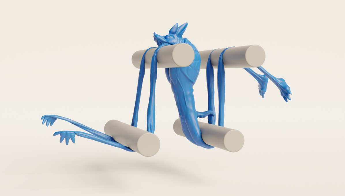
Figure 6. Robust contact handling in a simulation of an armadillo which is extremely deformed by animated cylinders.

Finally, we tested the contact energies in an experiment with extreme contact forces (see Fig. 6) to show that the system enables a robust contact handling. In this experiment an armadillo, modeled by linear tet elements and the Stable Neo-Hookean material, undergoes large deformations due to contact with animated rigid cylinders.

5.4. Adaptive Cloth Simulation

Figure 7. Our pipeline seamlessly handles changes in discretization, number of degrees of freedom and sparsity pattern in a cloth simulation with adaptive mesh refinement.

Adaptive mesh refinement cloth simulation.

We implemented a simulation using a non-linear material in combination with a quadratic bending model and strain limiting (see Fig. 7), in which we used an adaptive mesh refinement strategy to demonstrate that SymX can handle changes in discretization topology.

We use the Neo-Hookean strain energy for the cloth (using a 2D FEM integrator) and the quadratic bending energy proposed by Bergou et al. (2006)

(15) $$E_{b}(\boldsymbol{\mathbf{x}}_{e})=\frac{k_{b}}{2}\boldsymbol{\mathbf{x}}_{e}^{T}\boldsymbol{\mathbf{Q}}_{e}\boldsymbol{\mathbf{x}}_{e},$$

where $k_{b}$ is a stiffness coefficient, $\boldsymbol{\mathbf{x}}_{e}\in\mathbb{R}^{12}$ are the four unique mesh vertices of two adjacent triangles sharing a common internal edge $e$, and $\boldsymbol{\mathbf{Q}}_{e}\in\mathbb{R}^{12\times 12}$ is the internal edge quadratic form, which is constant during the simulation. Implementing this energy in our system requires a precomputation of the constant matrices $\boldsymbol{\mathbf{Q}}_{e}$ and just one line of code for the energy:

We employ a simple strain limiting model to avoid overstretching the cloth. While strain limiting can be implemented by restricting edge lengths to not extend beyond a threshold, as, e.g., shown by Narain et al. (2012), we opt for a continuous approach using the deformation gradient, as suggested, for instance, by Li et al. (2021). Note that the implementation effort of both approaches is almost identical when using our framework. The largest singular value $\sigma_{1}$ of the deformation gradient $\boldsymbol{\mathbf{F}}$ is used to measure the strain of a triangle, We employ a simple cubic penalty with user-defined stiffness $k_{sl}$ to enforce the constraint using a $C^{2}$ potential energy:

(16) $$E_{sl}(\boldsymbol{\mathbf{F}})=\begin{cases}\frac{k_{sl}}{3}A_{e}(\sigma_{1}(\boldsymbol{\mathbf{F}})-\sigma_{l})^{3}\quad&\text{if}\quad\sigma_{1}(\boldsymbol{\mathbf{F}})>\sigma_{l}\\ 0\quad&\text{if}\quad\sigma_{1}(\boldsymbol{\mathbf{F}})\leq\sigma_{l},\end{cases}$$

where $A_{e}$ is the undeformed area of the triangular element, $\sigma_{1}$ is the largest singular value of $\boldsymbol{\mathbf{F}}$ and $\sigma_{l}$ is the user-defined stretch limiting threshold. The largest singular value of a $2\times 2$ matrix can be computed using the direct method presented by Blinn (1996). Note in the experiment we used a rather low Young’s modulus of $200\text{\,}\mathrm{N}\mathrm{/}\mathrm{m}$ to investigate the effect of the strain limiting energy. The implementation just needs four lines of code in our system: Finally, for the adaptive mesh refinement we use a quadtree subdivision scheme that splits cells based on the divergence of the normals of the mesh vertices within the quadtree node. Although our refinement algorithm is rather simple, it suffices to show that SymX is capable of handling changes in the number of elements and the size of the arrays, including the one of the degrees of freedom.

5.5. Coupling Multiple Systems

The ability to couple multiple interacting physical systems, each one with its own list of degrees of freedom, is an important feature of our framework. This requires a global assembly method as described in Section 4.3.

In this section we show simulations with multiple coupled systems where a manual implementation of the derivatives and the logic code to put the simulation together would have taken a lot of time and effort. Our framework just requires the initial simulation data and one symbolic definition of each energy. This also makes it very easy to develop complex simulation systems with multiple people since energy definitions are independent from each other, enhancing productivity.

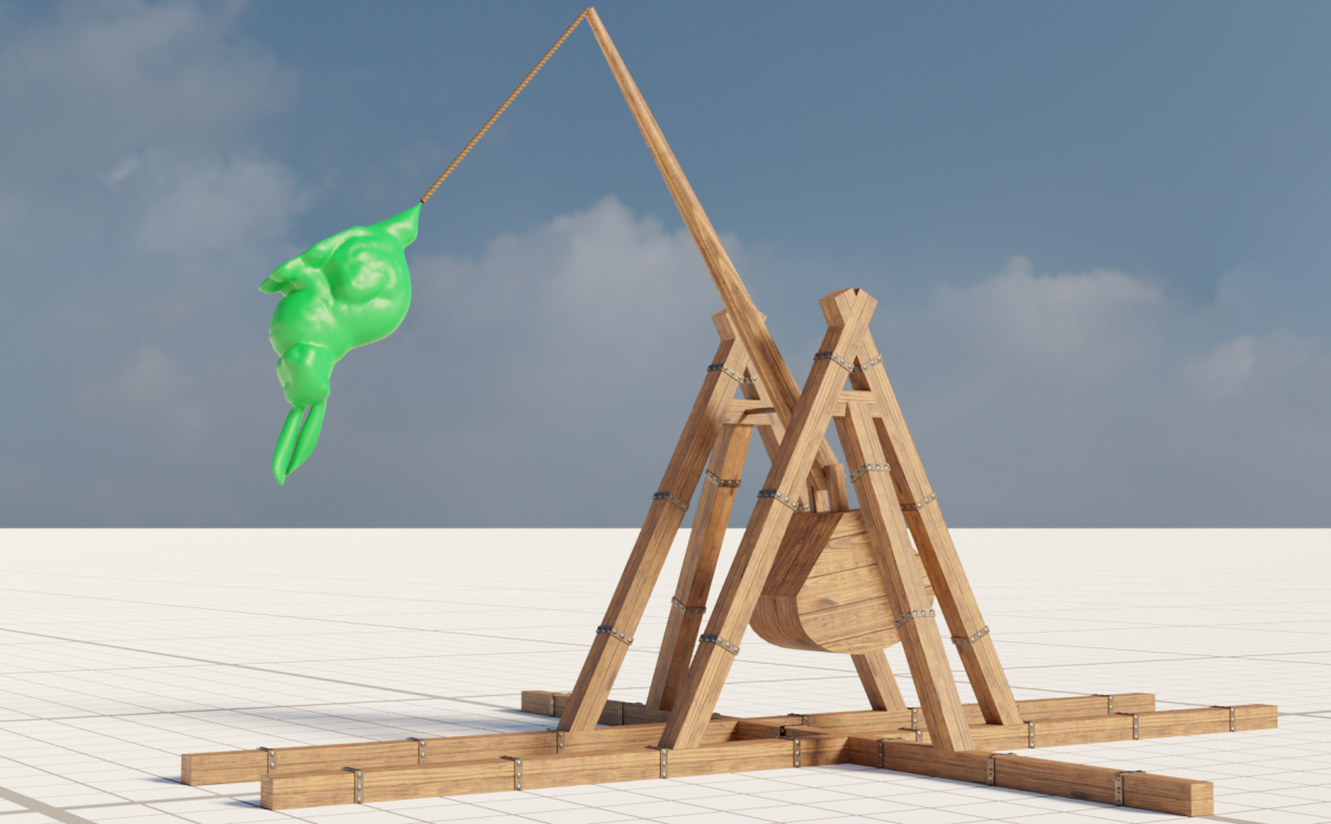
Figure 8. The trebuchet example couples a rigid body system for the trebuchet components with a system for deformable solids to throw an elastic bunny.

First, we simulated a car model (see Fig. 1) by coupling a rigid body system with joints and dampers with a deformable solid system for the tires. For the rigid body system we use the formulation presented by Macklin et al. (2020) for the inertia energy and formulate constraint energies using the penalty method

(17) $$E_{C}=\frac{1}{2}k_{C}C^{2},$$

where $k_{C}$ is the penalty stiffness and $C$ the constraint function. For two connector points $a$ and $b$ with global positions $\boldsymbol{\mathbf{x}}_{a}$, $\boldsymbol{\mathbf{x}}_{b}$, velocities $\boldsymbol{\mathbf{v}}_{a}$, $\boldsymbol{\mathbf{v}}_{b}$ and two normalized direction vectors $\boldsymbol{\mathbf{d}}_{a}$, $\boldsymbol{\mathbf{d}}_{b}$, we define ball joints, direction lock constraints, and slider joints as

(18) $$C^{2}_{bj}(\boldsymbol{\mathbf{x}}_{a},\boldsymbol{\mathbf{x}}_{b}) =\left\lVert\boldsymbol{\mathbf{x}}_{a}-\boldsymbol{\mathbf{x}}_{b}\right\rVert_{2}^{2}$$

(19) $$C^{2}_{dl}(\boldsymbol{\mathbf{d}}_{a},\boldsymbol{\mathbf{d}}_{b}) =\left\lVert\boldsymbol{\mathbf{d}}_{a}-\boldsymbol{\mathbf{d}}_{b}\right\rVert_{2}^{2}$$

(20) $$C^{2}_{sj}(\boldsymbol{\mathbf{x}}_{a},\boldsymbol{\mathbf{x}}_{b},\boldsymbol{\mathbf{d}}_{a}) =\left\lVert\boldsymbol{\mathbf{x}}_{b}-\boldsymbol{\mathbf{x}}_{a}-\left((\boldsymbol{\mathbf{x}}_{b}-\boldsymbol{\mathbf{x}}_{a})^{T}\boldsymbol{\mathbf{d}}_{a}\right)\boldsymbol{\mathbf{d}}_{a}\right\rVert_{2}^{2}.$$

Hinge joints are simply modeled by two ball joints. Additionally, the dampers of the car are implemented using the energy function of a damped spring

(21) $$\begin{split}E_{ds}(\boldsymbol{\mathbf{x}}_{a},\boldsymbol{\mathbf{x}}_{b},\boldsymbol{\mathbf{v}}_{a},\boldsymbol{\mathbf{v}}_{b})=&\frac{k_{sp}}{2}\left(\frac{\left\lVert\boldsymbol{\mathbf{x}}_{a}-\boldsymbol{\mathbf{x}}_{b}\right\rVert_{2}}{l_{0}}-1\right)^{2}+\\ &\frac{\alpha_{dp}}{2l_{0}}\left(\left(\boldsymbol{\mathbf{v}}_{a}-\boldsymbol{\mathbf{v}}_{b}\right)\cdot\frac{\boldsymbol{\mathbf{x}}_{a}-\boldsymbol{\mathbf{x}}_{b}}{\|\boldsymbol{\mathbf{x}}_{a}-\boldsymbol{\mathbf{x}}_{b}\|_{2}}\right)^{2},\end{split}$$

where $k_{sp}$ is the stiffness of the spring, $l_{0}$ its the rest length, and $\alpha_{dp}$ the damping coefficient.

Each wheel of the car has its own suspension system composed of multiple energies. A slider in combination with a damped spring models the damper of the car and attaches a rigid body to the chassis which is then linked by a hinge joint to the wheel rim to enable spinning. We use an additional hinge joint for each front wheel to steer the car. Unwanted relative rotations around the slider axes are eliminated by direction lock constraints, which are also used to steer the car. The tires are modeled by linear tet elements using the Stable Neo-Hookean material by Smith et al. (2018). Moreover, they are connected to the rims by attaching the tire mesh vertices which are closer than $1\text{\,}\mathrm{cm}$ to rim to the rigid body of the rim. Attachments between different physical systems are modeled analogous to the ball joints. Finally, contact and friction between the tires and the floor and obstacles is handled using the contact formulation introduced in Section 5.3.

In the second experiment we simulated a trebuchet (see Fig. 8) by coupling a rigid body system and a deformable solid system. It uses a mechanical compounded leverage to throw a soft bunny a long distance. To model the trebuchet we used ball joints and added a simple physical system for the string made of extensible segments. The bunny consists of linear finite elements in combination with the Stable Neo-Hookean material. Contacts are resolved with friction using the energies in Section 5.3.

6. Results

In this section we compare our framework with related approaches, and present experiments and benchmarks.

6.1. Discussion

In this section we discuss different approaches to compute the required first and second derivatives with respect to our requirements (automation, performance, productivity, and flexibility) defined in Section 1.

Manual implementation

The baseline option for many applications is to differentiate energies by hand and to manually implement and optimize the corresponding evaluation and assembly. While a thorough code optimization yields a high performance and the approach is flexible, it does not fulfill the other two requirements. Manual implementations are typically very time-consuming and hard to maintain. Moreover, changing an energy function in a simulator or adding a new one often takes much time.

Automatic differentiation

AD is often the solution of choice for many applications that require derivatives due to its flexibility. It is also commonly used for fast prototyping and testing. Therefore, AD fulfills most of our requirements. However, the performance of general purpose AD tools is too low for our application. AD excels at differentiating complex programs with arbitrary control flow that depend on a large number of variables. Our problem, however, is fundamentally different: we need derivatives of relatively compact closed mathematical expressions with respect to a low number of variables. Moreover, many AD libraries do not support second-order derivatives. After evaluating different tools in this field we find that TinyAD (Schmidt et al., 2022) is the best AD candidate for our problem. It is designed to compute the same type of derivatives that we also find in our applications, and it outperforms established AD libraries. To investigate if TinyAD also fulfills our performance requirement, we perform extensive performance comparisons with TinyAD in Section 6.

Symbolic off-the-shelf tools

Symbolic tools such as Mathematica (Wolfram Research, 2023) or SymPy (Meurer et al., 2017) can generate derivatives of arbitrary degree from mathematical expressions. However, to the best of our knowledge there is no high-performance symbolic differentiation solution that could be directly integrated in a simulation environment with our requirements. While some off-the-shelf tools can generate code for the derivatives, it typically has to be integrated manually into an existing simulation system. Therefore, this approach is not completely automatic and also the productivity requirement is not met due to time-consuming manual steps when changing or adding a new energy function to a simulation. Since the performance of such tools is still interesting for our work, we analyze the performance of code generated with SymPy (Meurer et al., 2017) and compare it to a manual solution and SymX in Section 6.2.

Numerical differentiation

While numerical differentiation has seen impressive advances in robustness and can provide reliable derivative information, for example with the Complex Step method (Luo et al., 2019), it still faces the fundamental problem that it requires multiple evaluations of the energy value itself, at least one for each entry in the gradient and Hessian. In our testing on a linear tetrahedral with a $12\times 12$ Hessian, evaluating the value of the energy was significantly more expensive than 1/144th of the runtime needed for the whole Hessian matrix. Therefore, we consider numerical differentiation unsuitable for our application.

Simulation systems and DSLs

While there is a plethora of relevant systems and Domain Specific Languages (DSL) as outlined in Section 2, we did not find a solution that fulfills all of our requirements. This is the original motivation behind the development of SymX. Most systems either do not support differentiation or only provide first-order derivatives. The most relevant approaches that do indeed support second-order derivatives are ACORNS (Desai et al., 2022) and the method by Herholz et al. (2022). ACORNS can generate Hessians that must be then manually integrated in the simulation but it does to not support dynamic branching and is outperformed by integrated solutions such as TinyAD. The method by Herholz et al., on the other hand, presents in fact very good performance by reducing and compiling all the sparse queries of the application into a single program, but this prohibits changes in the sparsity pattern and results in very long code generation and compilation times.

6.2. Benchmarks and timings

The following simulations and benchmarks were run on a workstation containing an AMD Ryzen Threadripper PRO 5975WX with 32 cores, $3.60$ GHz and $256$ GB of RAM. For further optimization we used AVX2 instructions for SIMD vectorization and OpenMP for multithreading. All simulations are executed with double precision, which equals to four floating point values per AVX2 instruction and fast-math for the benchmarks. Finally, we used version 10.2.1 of the gcc compiler.

We present two benchmarks to compare SymX, SymPy (Meurer et al., 2017), TinyAD (Schmidt et al., 2022), and an optimized manual implementation. Note that an expert took several hours to optimize the hand-written code while the implementation and automatic code generation with SymX and TinyAD just took minutes. The implementation using SymPy took longer since the generated code has to be integrated by hand in the simulator. In the comparisons we want to investigate if one of the automatically generated source codes is as fast as the highly-optimized code.

6.2.1. Single Element Benchmark

The first benchmark consists of repeatedly evaluating the stable Neo-Hookean energy (Smith et al., 2018), its gradient and its Hessian for a single linear, quadratic and cubic element, respectively. The results are shown in Table 1. TinyAD is the slowest method in all three cases. While automatic differentiation computes the expression and intermediate chain-rule derivatives at the same time, SymX generates unrolled code for the individual entries of the gradient and Hessian. This enables more extensive compiler optimization resulting in code that is not only up to $81x$ faster without and $207x$ faster with vectorization but also has a runtime in the same order of magnitude as hand-written optimized code. Moreover, we observe that the non-vectorized version of SymX is as fast as the implementation derived from SymPy. Both use the same fundamental method, thus we demonstrate that we do not add any overhead in the evaluation by automating the process. Furthermore, it also validates our symbolic differentiation implementation. Finally, while our non-vectorized, generated code is not as fast as well-optimized, hand-written code, we show that we can close the gap in performance by automatic vectorization.

Table 1. Benchmark of the evaluation time $t_{\mathrm{eval.}}$ of the stable Neo-Hookean energy, its gradient and Hessian with double precision for a single linear, quadratic and cubic finite element. Note that the timings are averaged and only SymX uses vectorization.

	linear	quadratic	cubic
Method	$t_{\mathrm{eval.}}[$\text{\,}\mathrm{\SIUnitSymbolMicro s}$]$	$t_{\mathrm{eval.}}[$\text{\,}\mathrm{\SIUnitSymbolMicro s}$]$	$t_{\mathrm{eval.}}[$\text{\,}\mathrm{\SIUnitSymbolMicro s}$]$
TinyAD	$7.40$	$402$	$5328$
Manual	$0.15$	$2.94$	$24.6$
SymPy	$0.24$	$6.25$	$63.0$
SymX (non-vec.)	$0.21$	$5.77$	$65.7$
SymX	$0.04$	$1.74$	$19.7$

6.2.2. Simulation Benchmark

In the following we perform a benchmark in a physical simulation setting. Thus, we compare the total time averaged over several time steps and Newton iterations. This includes the evaluation time of each energy and its derivatives as well as the global assembly. Note that for a fair comparison, we exchanged TinyAD’s triplet based sparse matrix assembly with our block based assembly which is significantly faster. In the simulation we stretched and twisted a cube with $59565$ degrees of freedom for all element types (see Fig. 5). Table 2 shows the results of the benchmark. As previously seen, TinyAD is again the slowest with SymX being up to $377x$ faster. The benchmark shows that the performance of the generated code with SymX is quite close to the manually highly optimized code. However, the development of the code was significantly easier and faster.

Table 2. Simulation benchmark of multiple iterations of a twisting cube example using linear, quadratic and cubic finite elements. The averaged timings include the evaluation of the energy and its derivative as well as the assembly. All simulation methods use our global assembly method in this benchmark.

	linear	quadratic	cubic
Method	$t_{\mathrm{total}}[$\text{\,}\mathrm{ms}$]$	$t_{\mathrm{total}}[$\text{\,}\mathrm{ms}$]$	$t_{\mathrm{total}}[$\text{\,}\mathrm{ms}$]$
SymX	$7.61$ $(x1.0)$	$9.80$ $(x1.0)$	$18.27$ $(x1.0)$
Manual	$6.06$ $(x0.80)$	$9.37$ $(x0.96)$	$15.86$ $(x0.87)$
TinyAD	$42.7$ $(x5.61)$	$251.1$ $(x25.62)$	$6890.6$ $(x377.15)$

6.2.3. Application Example Timings

In addition to these benchmarks, we also recorded timings of the application examples from Sec. 5 in Tab. 3. The time $t_{\mathrm{total}}$ includes the evaluation time for the energies and their derivatives, and the global assembly. All timings are normalized by the number of Newton iterations. Every example uses the Backward Euler integrator formulation used by Macklin et al. (2020) and an off-the-shelf conjugate gradient solver for the linear systems. Note that our system could easily be combined with any other integrator that admits an incremental potential formulation such as TR-BDF2 proposed by (Brown et al., 2018). The results show good scaling with an increasing number of degrees of freedom. Notably, in our application examples most of the time is spent during the linear system solve which is not part of SymX. Excluding it, most of the time is spent in assembly, while the evaluation only takes a minor fraction. For reference, we measure our included default BCRS assembly as $6x$ faster than building from triplets using Eigen.

Table 3. Simulation timings of the application examples from Sec. 5. Furthermore, the number of distinct, physical systems (rigid bodies, ropes, cloth, deformable solids) and the degrees of freedom are given.

Fig.	Scene	# Sys.	# DoF	$t_{\mathrm{total}}[$\text{\,}\mathrm{ms}$]$
4	ARAP	$1$	$307623$	$38.56$
4	Fixed Corot.	$1$	$307623$	$39.11$
4	StVK	$1$	$307623$	$42.84$
4	Neo-Hookean	$1$	$307623$	$37.66$
4	Stable NH	$1$	$307623$	$36.75$
5	Beam linear	$1$	$189$	$0.1$
5	Beam linear	$1$	$1728$	$0.27$
5	Beam linear	$1$	$11253$	$1.05$
5	Beam quadr.	$1$	$975$	$0.9$
5	Beam quadr.	$1$	$11253$	$1.85$
5	Beam quadr.	$1$	$80703$	$11.88$
5	Beam cubic	$1$	$2793$	$6.65$
5	Beam cubic	$1$	$35328$	$8.62$
5	Beam cubic	$1$	$262353$	$61.76$
6	Armadillo	$1$	$195510$	$34.18$
7	Adaptive cloth	$1$	$6339-24903$	$4.04$
1	Car Drifting	$2$	$17220$	$4.45$
8	Trebuchet	$3$	$23973$	$5.03$

6.2.4. Compilation Times

Finally, we also present the timings and memory requirements associated with differentiation and compilation in Table 4. Here, $T_{\mathrm{diff.}}$ denotes the total time needed for differentiating all the expressions in the simulation and $T_{\mathrm{comp.}}$ the time for gcc to compile the generated C++ code. Concerning the memory requirements, the peak memory column indicates the maximum storage needed during differentiation and the binary size, the sum of the sizes of the energies’ binaries. Timings for differentiation and compilation strongly correlate to expression complexity. The car scene for example contains many complex energy expressions and thus takes significantly longer than the stretched cubes. Furthermore, the choice of element has a significant impact. Finally, our memory requirements both in RAM during execution and disk space for the binaries are very modest. Additionally, our binaries are in the order of kilobytes in comparison to the gigabytes needed by Desai et al. (2022) or megabytes by Kjolstad et al. (2016).

Table 4. Measurements of the compile process. These include the timings of differentiation $T_{\mathrm{diff.}}$ and compiling $T_{\mathrm{comp.}}$. Note that for the latter, since multiple instances of the compiler are launched, the time is roughly equal to the most expensive energy compile time. Furthermore, the table contains the peak memory consumption, which reflects the computations related to symbols and the expression tree and the total size of the output binaries.

Fig.	Scene	$T_{\mathrm{diff.}}[$\text{\,}\mathrm{ms}$]$	$T_{\mathrm{comp.}}[$\text{\,}\mathrm{ms}$]$	Peak mem.	Binary size
4	ARAP	$16$	$872$	$55$ kB	$182.5$ kB
4	Fixed Corot.	$17$	$840$	$51$ kB	$178.5$ kB
4	StVK	$41$	$1121$	$94$ kB	$180.5$ kB
4	Neo-Hookean	$31$	$921$	$66$ kB	$182.6$ kB
4	Stable NH	$23$	$901$	$62$ kB	$182.6$ kB
5	Beam linear	$24$	$913$	$62$ kB	$182.6$ kB
5	Beam quadratic	$1453$	$5424$	$283$ kB	$260.4$ kB
5	Beam cubic	$23824$	$51565$	$1002$ kB	$498$ kB
6	Armadillo	$228$	$1699$	$453$ kB	$872.8$ kB
7	Adaptive cloth	$51$	$873$	$105$ kB	$383.3$ kB
1	Car	$236$	$1685$	$533$ kB	$1.0$ MB
8	Trebuchet	$246$	$1699$	$548$ kB	$1.2$ MB

7. Conclusions and Future Work

Many state-of-the-art simulation methods use a variant of Projected Newton (Gast et al., 2015; Li et al., 2020, 2021) to prevent Newton’s method from getting stuck due to indefiniteness of the global Hessian matrix. Here the element-local Hessian contributions are projected to semi-definiteness in some way. Our system can be used with Projected Newton by computing eigendecompositions of the element matrices. However, this may be more computationally expensive than state-of-the-art methods for deformable solids that rely on known properties of the eigenstructure of the material models themselves (Kim et al., 2019; Smith et al., 2019, 2018). We believe that the techniques we present in this paper could be enhanced with analytic eigenstructures to conveniently and efficiently differentiate material models defined in terms of scalar invariants.

Although we demonstrate that symbolic differentiation and code generation gets much closer to manually implemented code than the alternatives, there is still room for improvement. Our current system does not mathematically simplify the resulting derivative expressions besides avoiding redundant computation. It is possible that adding this kind of capability, as done in (Herholz et al., 2022), might help make the gap even smaller. In a similar spirit, directly supporting vectors and matrices in the expression graph instead of eagerly reducing all quantities to scalar operations might aid the search for more compact expressions.

Arguably the most significant limitation of symbolic and automatic differentiation is that some expressions, while differentiable, may contain partial expressions in their expression graph that are non-differentiable. Therefore, evaluating the result near a non-differentiable point in the intermediate expression may cause the intermediate result to become numerically unstable. Typically these kind of issues occur when the scalar expression contains norms, square roots or more generally fractional powers, as we have already seen in the symbolic definition of the friction energy, Section 5.3. Users may be taught to be wary of these issues in the presence of such expressions and apply workarounds like smooth approximations provided by the framework, but ultimately this is not foolproof. A mechanism for automatic reformulation of the expression to avoid such problems would be an important improvement. In the interim, we could augment our system to optionally detect such potential problems and notify the user, so that they may try a different formulation or use the stable operators provided.

In this work we presented SymX, a system to automate the differentiation and assembly in complex simulations based on optimization time integrators. SymX provides a set of symbolic types that allows engineers and researches to succinctly define the global energy of the simulation. Thanks to the link between these symbols and the simulation data, SymX can apply symbolic differentiation to the energies with respect to the degrees of freedom of the simulation and completely automate the assembly process. Thanks to on-the-fly compilation of the derivatives code, our method has a performance comparable to code optimized by hand.

We demonstrated the capabilities of our method in an array of different challenging simulations and show that the code required to express such simulation energies very closely resemble their original mathematical counterparts. In the view of the results obtained and the minimal code footprint needed by using SymX, we conclude that our system can indeed significantly boost productivity by allowing engineers to quickly compose and experiment with production-like performance. The flexibility of our method presents a path for an initial prototype to be gradually transitioned to a hybrid between symbolic and manual derivatives as the user sees fit. Finally, we are convinced that also other simulation methods like constraint-based approaches, or even applications in different fields like geometry processing, will benefit from our framework.

Appendix A Constitutive Models

References

(1)
Abadi et al. (2016)
Martín Abadi, Paul
Barham, Jianmin Chen, Zhifeng Chen,
Andy Davis, Jeffrey Dean,
Matthieu Devin, Sanjay Ghemawat,
Geoffrey Irving, Michael Isard,
Manjunath Kudlur, Josh Levenberg,
Rajat Monga, Sherry Moore,
Derek G. Murray, Benoit Steiner,
Paul Tucker, Vijay Vasudevan,
Pete Warden, Martin Wicke,
Yuan Yu, and Xiaoqiang Zheng.
2016.
TensorFlow: A System for Large-Scale Machine
Learning. In Proceedings of the 12th USENIX
Conference on Operating Systems Design and Implementation (Savannah, GA,
USA) (OSDI’16). USENIX
Association, USA, 265–283.
Andrews et al. (2022)
Sheldon Andrews, Kenny
Erleben, and Zachary Ferguson.
2022.
Contact and Friction Simulation for Computer
Graphics. In ACM SIGGRAPH 2022 Courses
(Vancouver, British Columbia, Canada) (SIGGRAPH
’22). Association for Computing Machinery,
New York, NY, USA, Article 3,
172 pages.
https://doi.org/10.1145/3532720.3535640
Bender et al. (2014)
Jan Bender, Kenny
Erleben, and Jeff Trinkle.
2014.
Interactive Simulation of Rigid Body Dynamics in
Computer Graphics.
Computer Graphics Forum
33, 1 (2014),
246–270.
Bergou et al. (2006)
Miklós Bergou, Max
Wardetzky, David Harmon, Denis Zorin,
and Eitan Grinspun. 2006.
A Quadratic Bending Model for Inextensible
Surfaces. In Proceedings of the Eurographics
Symposium on Geometry Processing(SGP ’06).
Eurographics Association, 227–230.
Bernstein et al. (2016)
Gilbert Louis Bernstein,
Chinmayee Shah, Crystal Lemire,
Zachary Devito, Matthew Fisher,
Philip Levis, and Pat Hanrahan.
2016.
Ebb: A DSL for Physical Simulation on CPUs and
GPUs.
ACM Trans. Graph. 35,
2, Article 21 (may
2016), 12 pages.
https://doi.org/10.1145/2892632
Blinn (1996)
J. Blinn. 1996.
Consider the lowly 2 x 2 matrix.
IEEE Computer Graphics and Applications
16, 2 (1996),
82–88.
https://doi.org/10.1109/38.486688
Bouaziz et al. (2014)
Sofien Bouaziz, Sebastian
Martin, Tiantian Liu, Ladislav Kavan,
and Mark Pauly. 2014.
Projective Dynamics: Fusing Constraint Projections
for Fast Simulation.
ACM Trans. Graph. 33,
4, Article 154 (jul
2014), 11 pages.
https://doi.org/10.1145/2601097.2601116
Brown et al. (2018)
George E. Brown, Matthew
Overby, Zahra Forootaninia, and Rahul
Narain. 2018.
Accurate dissipative forces in optimization
integrators.
ACM Transactions on Graphics
37, 6 (dec
2018), 1–14.
https://doi.org/10.1145/3272127.3275011
Chen et al. (2022)
Yunuo Chen, Minchen Li,
Lei Lan, Hao Su, Yin
Yang, and Chenfanfu Jiang.
2022.
A Unified Newton Barrier Method for Multibody
Dynamics.
ACM Trans. Graph. 41,
4, Article 66 (jul
2022), 14 pages.
https://doi.org/10.1145/3528223.3530076
Desai et al. (2022)
Deshana Desai, Etai
Shuchatowitz, Zhongshi Jiang, Teseo
Schneider, and Daniele Panozzo.
2022.
ACORNS: An easy-to-use code generator for gradients
and Hessians.
SoftwareX 17
(2022), 100901.
https://doi.org/10.1016/j.softx.2021.100901
DeVito et al. (2011)
Zachary DeVito, Niels
Joubert, Francisco Palacios, Stephen
Oakley, Montserrat Medina, Mike
Barrientos, Erich Elsen, Frank Ham,
Alex Aiken, Karthik Duraisamy,
Eric Darve, Juan Alonso, and
Pat Hanrahan. 2011.
Liszt: A Domain Specific Language for Building
Portable Mesh-Based PDE Solvers. In Proceedings of
2011 International Conference for High Performance Computing, Networking,
Storage and Analysis (Seattle, Washington) (SC
’11). Association for Computing Machinery,
New York, NY, USA, Article 9,
12 pages.
https://doi.org/10.1145/2063384.2063396
DeVito et al. (2017)
Zachary DeVito, Michael
Mara, Michael Zollhöfer, Gilbert
Bernstein, Jonathan Ragan-Kelley,
Christian Theobalt, Pat Hanrahan,
Matthew Fisher, and Matthias Niessner.
2017.
Opt: A Domain Specific Language for Non-Linear
Least Squares Optimization in Graphics and Imaging.
ACM Trans. Graph. 36,
5, Article 171 (oct
2017), 27 pages.
https://doi.org/10.1145/3132188
Gast et al. (2015)
Theodore Gast, Craig
Schroeder, Alexey Stomakhin, Chenfanfu
Jiang, and Joseph Teran.
2015.
Optimization Integrator for Large Time Steps.
IEEE Transactions on Visualization and
Computer Graphics 21, 10
(2015), 1103–1115.
Griewank and Walther (2008)
Andreas Griewank and
Andrea Walther. 2008.
Evaluating Derivatives: Principles and
Techniques of Algorithmic Differentiation (second ed.).
Society for Industrial and Applied Mathematics,
USA.
Herholz et al. (2022)
Philipp Herholz, Xuan
Tang, Teseo Schneider, Shoaib Kamil,
Daniele Panozzo, and Olga
Sorkine-Hornung. 2022.
Sparsity-Specific Code Optimization Using
Expression Trees.
ACM Trans. Graph. 41,
5, Article 175 (may
2022), 19 pages.
https://doi.org/10.1145/3520484
Hu et al. (2019)
Yuanming Hu, Tzu-Mao Li,
Luke Anderson, Jonathan Ragan-Kelley,
and Frédo Durand. 2019.
Taichi: A Language for High-Performance Computation
on Spatially Sparse Data Structures.
ACM Trans. Graph. 38,
6, Article 201 (nov
2019), 16 pages.
https://doi.org/10.1145/3355089.3356506
Jakob et al. (2022)
Wenzel Jakob,
Sébastien Speierer, Nicolas Roussel,
and Delio Vicini. 2022.
Dr.Jit: A Just-in-Time Compiler for Differentiable
Rendering.
ACM Trans. Graph. 41,
4, Article 124 (jul
2022), 19 pages.
https://doi.org/10.1145/3528223.3530099
Jia (2021)
Kai Jia. 2021.
SANM: A Symbolic Asymptotic Numerical Solver with
Applications in Mesh Deformation.
ACM Trans. Graph. 40,
4, Article 79 (jul
2021), 16 pages.
https://doi.org/10.1145/3450626.3459755
Karamouzas et al. (2017)
Ioannis Karamouzas, Nick
Sohre, Rahul Narain, and Stephen J.
Guy. 2017.
Implicit crowds: optimization integrator for robust
crowd simulation.
ACM Transactions on Graphics
36, 4 (jul
2017), 1–13.
https://doi.org/10.1145/3072959.3073705
Kharevych et al. (2006)
L. Kharevych, Weiwei
Yang, Y. Tong, E. Kanso,
J. E. Marsden, P. Schröder, and
M. Desbrun. 2006.
Geometric, Variational Integrators for Computer
Animation. In Proceedings of the 2006 ACM
SIGGRAPH/Eurographics Symposium on Computer Animation (Vienna, Austria)
(SCA ’06). Eurographics
Association, Goslar, DEU, 43–51.
Kim et al. (2019)
Theodore Kim, Fernando
De Goes, and Hayley Iben.
2019.
Anisotropic Elasticity for Inversion-Safety and
Element Rehabilitation.
ACM Trans. Graph. 38,
4, Article 69 (jul
2019), 15 pages.
https://doi.org/10.1145/3306346.3323014
Kjolstad et al. (2016)
Fredrik Kjolstad, Shoaib
Kamil, Jonathan Ragan-Kelley, David I. W.
Levin, Shinjiro Sueda, Desai Chen,
Etienne Vouga, Danny M. Kaufman,
Gurtej Kanwar, Wojciech Matusik, and
Saman Amarasinghe. 2016.
Simit: A Language for Physical Simulation.
ACM Trans. Graph. 35,
2, Article 20 (mar
2016), 21 pages.
https://doi.org/10.1145/2866569
Kugelstadt et al. (2018)
Tassilo Kugelstadt, Dan
Koschier, and Jan Bender.
2018.
Fast Corotated FEM using Operator Splitting.
Computer Graphics Forum
37, 8 (2018),
12 pages.
Li et al. (2020)
Minchen Li, Zachary
Ferguson, Teseo Schneider, Timothy
Langlois, Denis Zorin, Daniele Panozzo,
Chenfanfu Jiang, and Danny M. Kaufman.
2020.
Incremental Potential Contact: Intersection-and
Inversion-Free, Large-Deformation Dynamics.
ACM Trans. Graph. 39,
4, Article 49 (aug
2020), 20 pages.
https://doi.org/10.1145/3386569.3392425
Li et al. (2019)
Minchen Li, Ming Gao,
Timothy Langlois, Chenfanfu Jiang, and
Danny M. Kaufman. 2019.
Decomposed optimization time integrator for
large-step elastodynamics.
ACM Transactions on Graphics
38, 4 (jul
2019), 1–10.
https://doi.org/10.1145/3306346.3322951
Li et al. (2021)
Minchen Li, Danny M.
Kaufman, and Chenfanfu Jiang.
2021.
Codimensional Incremental Potential Contact.
ACM Trans. Graph. 40,
4, Article 170 (jul
2021), 24 pages.
https://doi.org/10.1145/3450626.3459767
Lin et al. (2022)
Huancheng Lin, Floyd M.
Chitalu, and Taku Komura.
2022.
Isotropic ARAP Energy Using Cauchy-Green
Invariants.
ACM Trans. Graph. 41,
6, Article 275 (nov
2022), 14 pages.
https://doi.org/10.1145/3550454.3555507
Luo et al. (2019)
Ran Luo, Weiwei Xu,
Tianjia Shao, Hongyi Xu, and
Yin Yang. 2019.
Accelerated Complex-Step Finite Difference for
Expedient Deformable Simulation.
ACM Trans. Graph. 38,
6, Article 160 (nov
2019), 16 pages.
https://doi.org/10.1145/3355089.3356493
Macklin et al. (2020)
M. Macklin, K. Erleben,
M. Müller, N. Chentanez,
S. Jeschke, and T. Y. Kim.
2020.
Primal/Dual Descent Methods for Dynamics. In
Proceedings of the ACM SIGGRAPH/Eurographics
Symposium on Computer Animation (Virtual Event, Canada)
(SCA ’20). Eurographics
Association, Goslar, DEU, Article 9,
12 pages.
https://doi.org/10.1111/cgf.14104
Mara et al. (2021)
Michael Mara, Felix
Heide, Michael Zollhöfer, Matthias
Nießner, and Pat Hanrahan.
2021.
Thallo – Scheduling for High-Performance
Large-Scale Non-Linear Least-Squares Solvers.
ACM Trans. Graph. 40,
5, Article 184 (sep
2021), 14 pages.
https://doi.org/10.1145/3453986
Martin et al. (2011)
Sebastian Martin, Bernhard
Thomaszewski, Eitan Grinspun, and
Markus Gross. 2011.
Example-based elastic materials.
ACM Transactions on Graphics
30, 4 (July
2011), 1.
https://doi.org/10.1145/2010324.1964967
Meurer et al. (2017)
Aaron Meurer,
Christopher P. Smith, Mateusz Paprocki,
Ondrej Certik, Sergey B. Kirpichev,
Matthew Rocklin, AMiT Kumar,
Sergiu Ivanov, Jason K. Moore,
Sartaj Singh, Thilina Rathnayake,
Sean Vig, Brian E. Granger,
Richard P. Muller, Francesco Bonazzi,
Harsh Gupta, Fredrik Vats,
Shivam andJohansson, Fabian Pedregosa,
Matthew J. Curry, Andy R. Terrel,
Stepan Roucka, Ashutosh Saboo,
Isuru Fernando, Sumith Kulal,
Robert Cimrman, and Anthony Scopatz.
2017.
SymPy: symbolic computing in Python.
PeerJ Computer Science 3
(Jan. 2017), e103.
https://doi.org/10.7717/peerj-cs.103
Narain et al. (2016)
Rahul Narain, Matthew
Overby, and George E. Brown.
2016.
ADMM Projective Dynamics: Fast
Simulation of General Constitutive Models. In ACM
SIGGRAPH/Eurographics Symposium on Computer Animation.
1–8.
Narain et al. (2012)
Rahul Narain, Armin
Samii, and James F. O’Brien.
2012.
Adaptive Anisotropic Remeshing for Cloth