MS-TP-23-05
Baryonic states in $\mathbf{\mathcal{N}=1}$ supersymmetric SU(2) Yang-Mills theory on the lattice

Abstract

Abstract: We extend our analysis of bound states in $\mathcal{N}=1$ supersymmetric Yang-Mills theory by the consideration of baryonic operators, which are composed of three gluino fields. The corresponding states are similar to the baryons in QCD, but due to the difference between gluino and quark fields, their properties and the fermion line contractions involved in their correlation functions are different from QCD. In this work, we first explain the derivation of these operators and the contractions needed in numerical calculations of their correlators. In contrast to QCD the correlators contain a spectacle piece, which requires methods for all-to-all propagators. We provide a first estimate of the two-point function and the mass of the lightest baryonic state in $\mathcal{N}=1$ supersymmetric Yang-Mills theory.

1 Introduction

Supersymmetry (SUSY) provides field theoretic models, which are interesting in view of various aspects of elementary particle theory. Supersymmetric extensions of the Standard Model are able to resolve the hierarchy problem [1], and they include dark matter candidates [2]. Supersymmetry enforces structural properties on models that can be investigated by perturbative or nonperturbative methods. This article addresses the $\mathcal{N}=1$ supersymmetric Yang-Mills (SYM) theory, which represents the supersymmetric extension of the gluonic sector of the Standard Model [3]. Gluons are described as usual by non-abelian gauge fields $A^{a}_{\mu}(x)$ for gauge group SU($N_{c}$), where $a=1,\ldots,N^{2}_{c}-1$. In addition to the gluons, SYM theory contains gluinos as their superpartners. Gluinos are Majorana fermions transforming under the adjoint representation of the gauge group. They are described by gluino fields $\lambda^{a}(x)$. In Minkowski space, the on-shell Lagrangian for $\mathcal{N}=1$ SYM theory, describing strongly interacting gluons and gluinos, is given by

$$\mathcal{L}_{\text{SYM}}=-\frac{1}{4}F^{a}_{\mu\nu}F^{a,\mu\nu}+\frac{\mathrm{i}}{2}\bar{\lambda}^{a}\gamma^{\mu}\left(\mathcal{D}_{\mu}\lambda\right)^{a}-\frac{m_{\tilde{g}}}{2}\bar{\lambda}^{a}\lambda^{a}.$$ (1)

Here $F^{a}_{\mu\nu}$ is the non-abelian field strength tensor, and $\mathcal{D}_{\mu}$ is the covariant derivative in the adjoint representation of the gauge group. The Lagrangian also includes a gluino mass term with mass $m_{\tilde{g}}$. For $m_{\tilde{g}}\neq 0$ this term breaks SUSY softly, which means that it does not affect the renormalisation properties of the theory and that the spectrum of the theory depends on the gluino mass in a continuous way.

In our previous investigations of SYM theory, we have concentrated on the low-lying mass spectrum of the theory with gauge group SU(2) and SU(3), which we have calculated nonperturbatively from first principles using Monte Carlo techniques [4, 5, 6, 7, 8]. In addition, we have studied the SUSY Ward identities [9, 10]. The particle spectrum of SYM theory is expected to consist of color neutral bound states of gluons and gluinos, which should form mass degenerate supermultiplets, if SUSY is not broken [11, 12]. In our numerical calculations, extrapolated to the continuum limit, we indeed obtain mass degenerate supermultiplets [8].

The predictions of [11, 12] for the low-lying supermultiplets are based on effective Lagrangeans, which describe bound states of two gluinos, bound states of a gluon and a gluino, and glueballs. Our previous numerical calculations have been focused on these types of particles. Due to the fact that gluinos are in the adjoint representation of the gauge group, it is, however, also possible for any number $N_{c}$ of colors to form color neutral bound states of three gluinos. As they are analogous to the baryons of QCD, we call these bound states generally “baryons”, even for gauge group SU(2), although bound states of $N_{c}$ fermions would commonly be called baryons.

Baryonic states in SYM theory have so far not being considered in the literature. It is the aim of this article to describe the theoretical framework for a numerical study of baryons in SYM theory, and to present the results of an explorative calculation.

Related baryonic states have been investigated in SU(2) Yang-Mills theory coupled to one Dirac fermion in the adjoint representation [13] with a different motivation from our study. In this case, there are conjectures about baryonic fields as dominant low energy degrees of freedom [14].

For the Monte-Carlo simulations on a Euclidean four-dimensional hypercubic lattice we use the action proposed by Curci and Veneziano [15]. The gauge part $S_{g}$ of the complete action $S=S_{g}+S_{f}$ is the usual plaquette action

$$S_{g}=-\frac{\beta}{N_{c}}\sum_{p}\mathrm{Re}\left[\mathrm{tr}\left(U_{p}\right)\right],$$ (2)

with the inverse gauge coupling given by $\beta=2N_{c}/g^{2}$. In the fermionic part $S_{f}$ the gluinos are implemented as Wilson fermions:

$$S_{f} =\frac{1}{2}\sum_{x}\left\{\bar{\lambda}^{a}_{x}\lambda_{x}^{a}-\kappa\sum_{\mu=1}^{4}\left[\bar{\lambda}^{a}_{x+\hat{\mu}}V_{ab,x\mu}(1+\gamma_{\mu})\lambda^{b}_{x}+\bar{\lambda}^{a}_{x}V^{T}_{ab,x\mu}(1-\gamma_{\mu})\lambda^{b}_{x+\hat{\mu}}\right]\right\}$$ (3)

$$\equiv\frac{1}{2}\sum_{x,y}\bar{\lambda}^{a}_{x}D_{w}^{ab}(x,y)\lambda_{y}^{b},$$ (4)

where $D_{w}$ is the Wilson-Dirac matrix. The link variables in the adjoint representation are given by $V_{ab,x\mu}=2\,\mathrm{tr}\,(U_{x\mu}^{\dagger}T_{a}U_{x\mu}T_{b})$, where $T_{a}$ are the generators of the gauge group. The hopping parameter $\kappa$ is related to the bare gluino mass $m_{\tilde{g}}$ by $\kappa=1/(2m_{\tilde{g}}+8)$. In order to approach the limit of vanishing gluino mass, the hopping parameter has to be tuned properly. In our numerical investigations the fermionic part is additionally $O(a)$ improved by adding the clover term $-(c_{sw}/4)\,\bar{\lambda}(x)\sigma_{\mu\nu}F^{\mu\nu}\lambda(x)$ [16].

2 Baryon correlation functions

2.1 Baryon operators

The mass of the lightest baryonic bound state in a channel specified by particular quantum numbers is obtained from the correlation function of a corresponding interpolating operator $W(x)$. Zero spatial momentum is enforced by summing over spatial coordinates,

$$W_{0}(t)=\sum_{\vec{x}}W(t,\vec{x}).$$ (5)

We consider local baryon operators $W(x)$ containing the product of three gluino fields $\lambda(x)$ at the same point $x$. A possible general construction, similar to the Rarita-Schwinger field [17], is

$$W(x)=t_{abc}\Gamma^{A}\lambda_{a}(x)\left(\lambda^{T}_{b}(x)\Gamma^{B}\lambda_{c}(x)\right),$$ (6)

where $\Gamma^{A}$ and $\Gamma^{B}$ are $4\times 4$ spin matrices, and $W(x)$ is a spinor. We choose $\Gamma^{A}=\mathbf{1}$ for simplicity, and denote $\Gamma^{B}=\Gamma$. In order that the baryon operator is a color singlet, $t_{abc}$ has to be an invariant color tensor. One choice would be the completely antisymmetric structure constants $f_{abc}$ of the gauge group. In the case of SU(2) this is the antisymmetric tensor $\varepsilon_{abc}$. The matrix $\Gamma$ has then to be symmetric, otherwise $W(x)$ would be zero identically due to the Grassmann nature of the gluino field. For SU(3) there is another choice, namely the symmetric color tensor $d_{abc}$. In this case $\Gamma$ has to be antisymmetric.

The spin of the baryon depends on the choice of $\Gamma$. Taking the Majorana condition

$$\bar{\lambda}(x)=\lambda^{T}(x)C$$ (7)

into account, where $C$ is the charge conjugation matrix, the factor $\lambda^{T}_{b}(x)\Gamma\lambda_{c}(x)$ transforms as a singlet under spatial rotations for $\Gamma=C\gamma_{4},C\gamma_{5},\mathrm{i}\gamma_{4}C\gamma_{5}$. Consequently, for these choices $W(x)$ describes a baryon with spin 1/2. On the other hand, for $\Gamma=C\gamma_{i}$, $i=1,2,3$, the factor $\lambda^{T}_{b}(x)\Gamma\lambda_{c}(x)$ transforms as a spatial vector, and $W(x)$ will in general contain spin 3/2 and spin 1/2 contributions [18]. The projections to definite spin are involved and are discussed in [19].

2.2 Baryonic correlation functions

The correlation functions, needed for the computation of baryon masses, are obtained from the interpolating field $W(x)$ and its conjugate field $\overline{W}(x)$ as

$$B(x,y)=\braket{W(x)\overline{W}(y)},$$ (8)

where $\overline{W}(x)$ is given by

$$\overline{W}(x)=\left(CW(x)\right)^{T}$$ (9)

up to a sign depending on the choice of the spin matrix [20]. With explicit Dirac indices the correlation function reads

$$B^{\alpha\delta}(x,y) =\langle W^{\alpha}(x)\overline{W}^{\delta}(y)\rangle=\langle W^{\alpha}(x)C^{\delta\alpha^{\prime}}W^{\alpha^{\prime}}(y)\rangle$$

$$=t_{abc}t_{a^{\prime}b^{\prime}c^{\prime}}\Gamma^{\beta\gamma}\Gamma^{\beta^{\prime}\gamma^{\prime}}C^{\delta\alpha^{\prime}}\,\langle\lambda_{a}^{\alpha}(x)\lambda_{b}^{\beta}(x)\lambda_{c}^{\gamma}(x)\lambda_{a^{\prime}}^{\alpha^{\prime}}(y)\lambda_{b^{\prime}}^{\beta^{\prime}}(y)\lambda_{c^{\prime}}^{\gamma^{\prime}}(y)\rangle.$$ (10)

In the numerical calculations the fermionic expectation values

$$\langle\mathcal{O}\rangle_{F}=\int\!\!D\lambda\ \mathcal{O}\,\mathrm{e}^{-S_{f}}$$ (11)

in a given gauge field background are needed. By Wick’s theorem they can be expressed in terms of the gluino two-point function

$$K^{\alpha\beta}_{ab}(x,y)=\langle\lambda^{\alpha}_{a}(x)\lambda^{\beta}_{b}(y)\rangle_{F}.$$ (12)

The antisymmetric matrix $K$ is related to the gluino propagator by

$$K^{\alpha\beta}_{ab}(x,y)=-\left(\Delta(x,y)C\right)^{\alpha\beta}_{ab},$$ (13)

where the propagator $\Delta=D_{w}^{-1}$ is the inverse of the Wilson-Dirac matrix $D_{w}$. For the product of six gluino fields, taking into account the fermionic signs, we get the following 15 terms:

$$\langle\lambda_{a}^{\alpha}(x)\lambda_{b}^{\beta}(x)\lambda_{c}^{\gamma}(x)\lambda_{a^{\prime}}^{\alpha^{\prime}}(y)\lambda_{b^{\prime}}^{\beta^{\prime}}(y) \lambda_{c^{\prime}}^{\gamma^{\prime}}(y)\rangle_{F}=$$

$$+K^{\alpha\beta}_{ab}(x,x)K^{\gamma\alpha^{\prime}}_{ca^{\prime}}(x,y)K^{\beta^{\prime}\gamma^{\prime}}_{b^{\prime}c^{\prime}}(y,y)$$

$$-K^{\alpha\beta}_{ab}(x,x)K^{\gamma\beta^{\prime}}_{cb^{\prime}}(x,y)K^{\alpha^{\prime}\gamma^{\prime}}_{a^{\prime}c^{\prime}}(y,y)$$

$$+K^{\alpha\beta}_{ab}(x,x)K^{\gamma\gamma^{\prime}}_{cc^{\prime}}(x,y)K^{\alpha^{\prime}\beta^{\prime}}_{a^{\prime}b^{\prime}}(y,y)$$

$$-K^{\alpha\gamma}_{ac}(x,x)K^{\beta\alpha^{\prime}}_{ba^{\prime}}(x,y)K^{\beta^{\prime}\gamma^{\prime}}_{b^{\prime}c^{\prime}}(y,y)$$

$$+K^{\alpha\gamma}_{ac}(x,x)K^{\beta\beta^{\prime}}_{bb^{\prime}}(x,y)K^{\alpha^{\prime}\gamma^{\prime}}_{a^{\prime}c^{\prime}}(y,y)$$

$$-K^{\alpha\gamma}_{ac}(x,x)K^{\beta\gamma^{\prime}}_{bc^{\prime}}(x,y)K^{\alpha^{\prime}\beta^{\prime}}_{a^{\prime}b^{\prime}}(y,y)$$

$$+K^{\alpha\alpha^{\prime}}_{aa^{\prime}}(x,y)K^{\beta\gamma}_{bc}(x,x)K^{\beta^{\prime}\gamma^{\prime}}_{b^{\prime}c^{\prime}}(y,y)$$

$$-K^{\alpha\alpha^{\prime}}_{aa^{\prime}}(x,y)K^{\beta\beta^{\prime}}_{bb^{\prime}}(x,y)K^{\gamma\gamma^{\prime}}_{cc^{\prime}}(x,y)$$

$$+K^{\alpha\alpha^{\prime}}_{aa^{\prime}}(x,y)K^{\beta\gamma^{\prime}}_{bc^{\prime}}(x,y)K^{\gamma\beta^{\prime}}_{cb^{\prime}}(x,y)$$

$$-K^{\alpha\beta^{\prime}}_{ab^{\prime}}(x,y)K^{\beta\gamma}_{bc}(x,x)K^{\alpha^{\prime}\gamma^{\prime}}_{a^{\prime}c^{\prime}}(y,y)$$

$$+K^{\alpha\beta^{\prime}}_{ab^{\prime}}(x,y)K^{\beta\alpha^{\prime}}_{ba^{\prime}}(x,y)K^{\gamma\gamma^{\prime}}_{cc^{\prime}}(x,y)$$

$$-K^{\alpha\beta^{\prime}}_{ab^{\prime}}(x,y)K^{\beta\gamma^{\prime}}_{bc^{\prime}}(x,y)K^{\gamma\alpha^{\prime}}_{ca^{\prime}}(y,y)$$

$$+K^{\alpha\gamma^{\prime}}_{ac^{\prime}}(x,y)K^{\beta\gamma}_{bc}(x,x)K^{\alpha^{\prime}\beta^{\prime}}_{a^{\prime}b^{\prime}}(y,y)$$

$$-K^{\alpha\gamma^{\prime}}_{ac^{\prime}}(x,y)K^{\beta\alpha^{\prime}}_{ba^{\prime}}(x,y)K^{\gamma\beta^{\prime}}_{cb^{\prime}}(x,y)$$

$$+K^{\alpha\gamma^{\prime}}_{ac^{\prime}}(x,y)K^{\beta\beta^{\prime}}_{bb^{\prime}}(x,y)K^{\gamma\alpha^{\prime}}_{ca^{\prime}}(x,y).$$ (14)

In the correlation function some of these terms can be combined, using the fact, that $t_{abc}$ is totally antisymmetric and $\Gamma^{\beta\gamma}$ is symmetric, or vice versa. We are then left with

$$B^{\alpha\delta}(x,y)=t_{abc}t_{a^{\prime}b^{\prime}c^{\prime}} \Gamma^{\beta\gamma}\Gamma^{\beta^{\prime}\gamma^{\prime}}C^{\delta\alpha^{\prime}}$$

$$\{ -2K^{\alpha\alpha^{\prime}}_{aa^{\prime}}(x,y)K^{\beta\beta^{\prime}}_{bb^{\prime}}(x,y)K^{\gamma\gamma^{\prime}}_{cc^{\prime}}(x,y)$$

$$-4K^{\alpha\beta^{\prime}}_{ab^{\prime}}(x,y)K^{\beta\gamma^{\prime}}_{bc^{\prime}}(x,y)K^{\gamma\alpha^{\prime}}_{ca^{\prime}}(x,y)$$

$$-2K^{\alpha\beta}_{ab}(x,x)K^{\gamma\alpha^{\prime}}_{ca^{\prime}}(x,y)K^{\gamma^{\prime}\beta^{\prime}}_{c^{\prime}b^{\prime}}(y,y)$$

$$-4K^{\alpha\beta}_{ab}(x,x)K^{\beta^{\prime}\gamma}_{b^{\prime}c}(y,x)K^{\gamma^{\prime}\alpha^{\prime}}_{c^{\prime}a^{\prime}}(y,y)$$

$$-1K^{\alpha\alpha^{\prime}}_{aa^{\prime}}(x,y)K^{\beta\gamma}_{bc}(x,x)K^{\gamma^{\prime}\beta^{\prime}}_{c^{\prime}b^{\prime}}(y,y)$$

$$+2K^{\alpha\beta^{\prime}}_{ab^{\prime}}(x,y)K^{\beta\gamma}_{bc}(x,x)K^{\gamma^{\prime}\alpha^{\prime}}_{c^{\prime}a^{\prime}}(y,y)\}.$$ (15)

In the special case $\Gamma=C\gamma_{4}$, which we consider in our numerical work, expressing the correlation function in terms of the propagator leads to

$$B^{\alpha\alpha^{\prime}}(x,y)=-f_{abc}f_{a^{\prime}b^{\prime}c^{\prime}} (C\gamma_{4})^{\beta\gamma}(C\gamma_{4})^{\beta^{\prime}\gamma^{\prime}}$$

$$\{ +2\Delta^{\alpha\alpha^{\prime}}_{aa^{\prime}}(x,y)\Delta^{\beta\beta^{\prime}}_{bb^{\prime}}(x,y)\Delta^{\gamma\gamma^{\prime}}_{cc^{\prime}}(x,y)$$

$$+4\Delta^{\alpha\beta^{\prime}}_{ab^{\prime}}(x,y)\Delta^{\beta\gamma^{\prime}}_{bc^{\prime}}(x,y)\Delta^{\gamma\alpha^{\prime}}_{ca^{\prime}}(x,y)$$

$$+2\Delta^{\alpha\beta}_{ab}(x,x)\Delta^{\delta\alpha^{\prime}}_{ca^{\prime}}(x,y)\Delta^{\delta^{\prime}\beta^{\prime}}_{c^{\prime}b^{\prime}}(y,y)C^{\gamma\delta}C^{\delta^{\prime}\gamma^{\prime}}$$

$$+4\Delta^{\alpha\beta}_{ab}(x,x)\Delta^{\beta^{\prime}\gamma}_{b^{\prime}c}(y,x)\Delta^{\gamma^{\prime}\alpha^{\prime}}_{c^{\prime}a^{\prime}}(y,y)$$

$$+1\Delta^{\alpha\alpha^{\prime}}_{aa^{\prime}}(x,y)\Delta^{\beta\delta}_{bc}(x,x)\Delta^{\delta^{\prime}\beta^{\prime}}_{c^{\prime}b^{\prime}}(y,y)C^{\gamma\delta}C^{\delta^{\prime}\gamma^{\prime}}$$

$$+2\Delta^{\alpha\delta^{\prime}}_{ac^{\prime}}(x,y)\Delta^{\beta\delta}_{bc}(x,x)\Delta^{\beta^{\prime}\alpha^{\prime}}_{b^{\prime}a^{\prime}}(y,y)C^{\gamma\delta}C^{\delta^{\prime}\gamma^{\prime}}\}.$$ (16)

With respect to the dependence on the space-time coordinates the first two terms are summed up to the sunset contribution $B_{\textrm{Sset}}(x,y)$, and the remaining four terms to the spectacle contribution $B_{\textrm{Spec}}(x,y)$, whose graphical representations are given in Fig. (1).

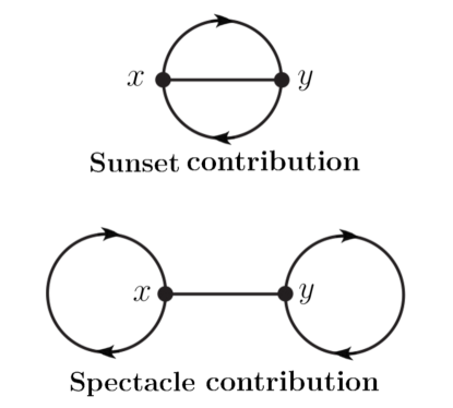
Figure 1: The “Sunset” and “Spectacle” contributions to the baryon correlation function in SYM theory.

According to the availability of gauge ensembles and to obtain first result for baryon masses, it is numerically less expensive and convenient to consider gauge group SU(2). In this case the baryon operator contains the antisymmetric structure constants $t_{abc}=\varepsilon_{abc}$, and the spin matrix $\Gamma$ has to be symmetric. We consider the choice $\Gamma=C\gamma_{4}$.

For zero momentum states, projection to definite parity can be accomplished with the projection operators $P_{\pm}=\frac{1}{2}(1\pm\gamma_{4})$ [21]. This finally gives

$$B^{\pm}_{\textrm{Sset}}(x,y)=-\varepsilon_{abc}\varepsilon_{a^{\prime}b^{\prime}c^{\prime}} (C\gamma_{4})^{\beta\gamma}(C\gamma_{4})^{\beta^{\prime}\gamma^{\prime}}P_{\pm}^{\alpha\alpha^{\prime}}$$

$$\langle +2\Delta^{\alpha\alpha^{\prime}}_{aa^{\prime}}(x,y)\Delta^{\beta\beta^{\prime}}_{bb^{\prime}}(x,y)\Delta^{\gamma\gamma^{\prime}}_{cc^{\prime}}(x,y)$$

$$+4\Delta^{\alpha\beta^{\prime}}_{ab^{\prime}}(x,y)\Delta^{\beta\gamma^{\prime}}_{bc^{\prime}}(x,y)\Delta^{\gamma\alpha^{\prime}}_{ca^{\prime}}(x,y)\rangle,$$ (17)

and

$$B^{\pm}_{\textrm{Spec}}(x,y)=-\varepsilon_{abc}\varepsilon_{a^{\prime}b^{\prime}c^{\prime}} (C\gamma_{4})^{\beta\gamma}(C\gamma_{4})^{\beta^{\prime}\gamma^{\prime}}P_{\pm}^{\alpha\alpha^{\prime}}$$

$$\langle +2\Delta^{\alpha\beta}_{ab}(x,x)\Delta^{\delta\alpha^{\prime}}_{ca^{\prime}}(x,y)\Delta^{\delta^{\prime}\beta^{\prime}}_{c^{\prime}b^{\prime}}(y,y)C^{\gamma\delta}C^{\delta^{\prime}\gamma^{\prime}}$$

$$+4\Delta^{\alpha\beta}_{ab}(x,x)\Delta^{\beta^{\prime}\gamma}_{b^{\prime}c}(y,x)\Delta^{\gamma^{\prime}\alpha^{\prime}}_{c^{\prime}a^{\prime}}(y,y)$$

$$+1\Delta^{\alpha\alpha^{\prime}}_{aa^{\prime}}(x,y)\Delta^{\beta\delta}_{bc}(x,x)\Delta^{\delta^{\prime}\beta^{\prime}}_{c^{\prime}b^{\prime}}(y,y)C^{\gamma\delta}C^{\delta^{\prime}\gamma^{\prime}}$$

$$+2\Delta^{\alpha\delta^{\prime}}_{ac^{\prime}}(x,y)\Delta^{\beta\delta}_{bc}(x,x)\Delta^{\beta^{\prime}\alpha^{\prime}}_{b^{\prime}a^{\prime}}(y,y)C^{\gamma\delta}C^{\delta^{\prime}\gamma^{\prime}}\rangle.$$ (18)

3 Numerical results

We have investigated the baryonic states in $\mathcal{N}=1$ supersymmetric Yang-Mills theory with gauge group SU(2) by means of numerical Monte Carlo techniques. The correlation functions have been calculated based on configurations produced in previous work [4, 23].

As explained in the previous section, the baryon correlator consists of a sunset and a spectacle contribution that require different numerical methods. In both cases, the inverse of the Wilson-Dirac operator is required, which is provided by standard iterative solvers for a given input vector.

In the sunset contribution, all propagators connect the two lattice points and a point source can be chosen for the inversion. To complete the contractions, this has to be repeated for all spin and color indices on the source side.

The spectacle part contains closed loop contributions ($\Delta(x,x)$ and $\Delta(y,y)$), in which the propagator connects each point with itself. These require techniques for a stochastic estimation of all-to-all propagators. We have already applied similar techniques for the estimation of mesonic operators in SYM. The inversion is done for several stochastic source vectors, which leads to an additional noise contribution in the signal. In practice we use 40 stochastic estimators combined with the exact contribution of the 200 lowest eigenmodes of $\gamma_{5}D_{W}$.

The spectacle contribution combines the loops at $x$ and $y$ with a propagator. This is done by an inversion with a wall source vector at a time slice $x_{0}$ filled with appropriate entries from the stochastically estimated loop ($\Delta(x,x)$). The resulting sink vector is consequently contracted with the loop ($\Delta(y,y)$) at different time slices $y_{0}$. The whole procedure is repeated for all source time slices $x_{0}$ to get the best signal for the average correlator $B(y_{0},x_{0})$.

3.1 Discrete symmetries of the correlation functions

To cross-check the correctness of the numerical data for the correlation function of Eq. (16), discrete symmetries for time reversal ($\mathcal{T}$) and parity ($\mathcal{P}$) are used  [19, 22]. The baryon correlation function transforms according to

$$\!\!\!\!\!\!B(x,y)\! \rightarrow \!B^{\mathcal{P}}(x^{\mathcal{P}},y^{\mathcal{P}})\!=\!\braket{W^{\mathcal{P}}(x^{\mathcal{P}})\overline{W}^{\mathcal{P}}(y^{\mathcal{P}})}\!=\!\gamma_{4}B(x^{\mathcal{P}},y^{\mathcal{P}})\gamma_{4},$$ (19)

$$\!\!\!\!\!\!B(x,y)\! \rightarrow \!B^{\mathcal{T}}(x^{\mathcal{T}},y^{\mathcal{T}})\!=\!\braket{W^{\mathcal{T}}(x^{\mathcal{T}})\overline{W}^{\mathcal{T}}(y^{\mathcal{T}})}\!=\!\gamma_{4}\gamma_{5}B(x^{\mathcal{T}},y^{\mathcal{T}})\gamma_{5}\gamma_{4}.$$ (20)

We consider the zero spatial momentum correlation function

$$B(t)=\sum\limits_{\begin{subarray}{c}\vec{x},\vec{y}\\ t=x_{0}-y_{0}\end{subarray}}B(x,y).$$ (21)

With the help of $\gamma_{5}$-hermiticity of the Wilson-Dirac matrix we arrive at

$$B_{\boldsymbol{1}}(t) =-B_{\boldsymbol{1}}(N_{t}-t),$$ (22)

$$B_{\gamma_{4}}(t) =B_{\gamma_{4}}(N_{t}-t),$$ (23)

where $B_{\boldsymbol{1}}(t)=\frac{1}{4}\mathrm{tr}\left[B(t)\right]$, $B_{\gamma_{4}}(t)=\frac{1}{4}\mathrm{tr}\left[B(t)\gamma_{4}\right]$, and $N_{t}$ is the time extent of the lattice.

We have checked these symmetries for the sunset contributions, for which much more precise numerical results are available compared to the spectacle contributions. Fig. (2) confirms that the sunset contribution of $B_{\boldsymbol{1}}(t)$ is antisymmetric, and the one of $B_{\gamma_{4}}(t)$ is symmetric within errors.

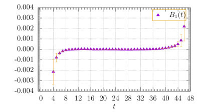
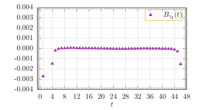
Figure 2: Numerical results for the sunset contributions of the correlation functions $B_{\boldsymbol{1}}(t)$ and $B_{\gamma_{4}}(t)$ at $\beta$=1.75 and $\kappa=0.14925$ for gauge group SU(2).

3.2 Baryonic correlation functions and masses

The numerical results of this exploratory study have been obtained for one ensemble of SU(2) SYM presented in [4, 23]. The lattice has size $24^{3}\times 48$, and the parameters are $\beta=1.75$ and $\kappa=0.14925$. A tree level Symanzik improved gauge action and a Wilson-Dirac operator with one level stout smeared links has been applied.

The resulting propagators for positive and negative parity with their respective sunset and spectacle contributions are presented in Fig. 3. A standard Jackknife procedure has been applied for error estimation.

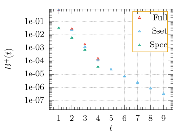
(a) Positive parity correlator.

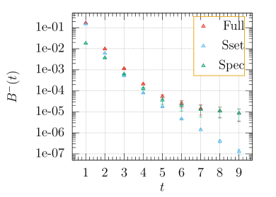
(b) Negative parity correlator.

Figure 3: Numerical results for the baryon correlation functions for (a) positive parity and (b) negative parity at $\beta=1.75$ and $\kappa=0.14925$ on a $24^{3}\times 48$ lattice. In addition to the full correlators, the sunset (“Sset”) and spectacle (“Spec”) contributions are shown.

The sunset contribution provides a much better signal than the spectacle one for all of the correlators. This contribution is similar to baryonic operators in QCD and hence an accuracy comparable with QCD data is achieved. In SYM, however, the sunset contribution does not correspond to the correlator of a particle state. Only in a theory with a larger number of fermion species the sunset contribution is related to a physical bound state. In this sense the sunset contribution in SYM can be considered as a partially quenched approximation to a particle correlator. The sunset contribution can be fitted quite accurately to a single exponential for both parities. The corresponding masses are rather large compared to the meson masses, see Tab. 1.

$am_{B^{+}_{\textrm{Sset}}}$	$am_{B^{-}_{\textrm{Sset}}}$	$am_{B^{-}}$	$am_{\text{a-}\pi}$	$am_{g\tilde{g}}$	$am_{\text{a-}\eta^{\prime}}$
1.020(47)	1.207(82)	0.24(18)	0.20381(80)	0.3740(75)	0.299(28)

Table 1: Masses of the baryon and two-particle bound states [4] in $\mathcal{N}$=1 SUSY Yang-Mills theory with gauge group SU(2) for $\beta=1.75$ and $\kappa=0.14925$.

The complete correlators are obtained by adding the spectacle contributions, which are much more noisy. The negative parity channel of the complete correlator provides a sufficient signal for an estimation the mass. An estimation of the positive parity mass has, however, not been possible with the current data.

The negative parity state appears to be significantly lighter than the one obtained considering only the sunset contribution. The estimation of the lightest mass is in this case rather challenging since there seems to be a large excited state contribution, i. e. the prefactor of its exponential is quite large. In the following we explain the methods used to obtain the result for the negative parity state of Tab. 1.

As a first test we have assumed a single exponential form of the correlator to obtain an effective mass at two lattice points. An estimate for the mass averaging these data in the range $t\in[6,8]$ would be around $m_{B^{-}}=0.31(35)$. The masses obtained from a single exponential fit in different $t$-ranges are summarized in Tab. 2. This mass estimate seems to decrease at larger $t$ towards values below $0.3$, but at the same time the signal gets overwhelmed by the error. A possible estimate is $m_{B^{-}}=0.31(18)$ from the fit interval $t\in[6,9]$. This is an indication that excited state contamination is rather large at the accessible $t$-range of the correlator.

Fit range ($t$)	$A$	$\sigma_{A}$	$m$	$\sigma_{m}$
6–8	1.54856e-04	2.76203e-04	0.32236	0.25463
6–9	1.42584e-04	2.00976e-04	0.31265	0.18452
7–9	9.98849e-05	2.17467e-04	0.26426	0.28608

Table 2: Estimates of the mass $m$ and multiplicative factor $A$ for negative parity using the fit function $A\,\mathrm{e}^{-mt}$. The errors are denoted by $\sigma$.

In order to remove the excited state contamination, we have done double exponential fits. The results in Tab. 3 and 4 show that this provides more consistent data even at smaller $t$ ranges compared to the single exponential fit. A mass estimate is $m_{B^{-}}=0.24(18)$ from the fit interval $t\in[3,9]$. As can be seen from the values of the prefactor $A_{1}$ in Tab. 4, there is a large contribution from the heavy mass of the excited state.

Fit range ($t$)	$m_{1}$	$\sigma_{m_{1}}$	$m$	$\sigma_{m}$
3–7	1.82570	0.12008	0.28226	0.42181
3–8	1.80280	0.09764	0.21303	0.24616
3–9	1.81288	0.09521	0.24190	0.17894
4–8	1.69159	0.65843	0.13819	0.58371
4–9	1.78465	0.57213	0.22977	0.29006

Table 3: Masses are estimated by fitting the function $A_{1}\,\mathrm{e}^{-m_{1}t}+A\,\mathrm{e}^{-mt}$ to the correlator data for different fit ranges (negative parity).

Fit range ($t$)	$A_{1}$	$\sigma_{A_{1}}$	$A$	$\sigma_{A}$
3–7	2.61276e-01	8.32151e-02	1.10252e-04	3.40647e-04
3–8	2.46011e-01	6.60862e-02	6.56622e-05	1.16709e-04
3–9	2.52735e-01	6.70216e-02	7.83048e-05	1.09974e-04
4–8	1.79004e-01	5.58144e-01	4.40431e-05	1.71411e-04
4–9	2.43887e-01	6.00709e-01	7.41955e-05	1.71981e-04

Table 4: The parameters $A$ and $A_{1}$ for the fits in Tab. 3.

We have tested further methods like a fit of the excited state contamination using only the sunset part, but without reasonable improvement. Our final best estimates in Tab. 1 have been obtained from a multistate fit analysis which uses the $\cosh$ function and Akaike information criterion (AIC) explained in [24] and references therein. Note that all methods provide results consistent within the errors.

4 Conclusion

We have presented a discussion of baryonic bound states in $\mathcal{N}=1$ supersymmetric Yang-Mills theory. It is usually not expected that these are part of the lightest multiplets of the theory. These states are similar to baryonic states of QCD, but their correlators have a different type of contractions and require a spectacle contribution in addition to the usual sunset diagrams.

We have done a first exploratory numerical study of correlators and particle masses for these bound states. The sunset contribution alone leads to a rather heavy particle mass. It is quite challenging to provide a reasonable result including the spectacle contribution due to the small signal to noise ratio. Our first estimates suggest a mass in the negative parity channel which is compatible with the lightest multiplet. This might be due to an overlap with the gluino-glue bound state, which is the fermionic member of the lightest multiplet.

Further improvements of the measurement are possible. The most relevant one is a detailed analysis of smearing methods to reduce the overlap with excited states. We plan to test this in a subsequent analysis of the SYM spectrum.

References

• [1] J. D. Lykken, [arXiv: 1005.1676[hep-ph]].
• [2] G. Jungman, M. Kamionkowski and K. Griest, Phys. Rept. 267 (1996) 195, [arXiv: hep-ph/9506380 ].
• [3] D. Amati, K. Konishi, Y. Meurice, G. C. Rossi and G. Veneziano, Phys. Rept. 162 (1988) 169.
• [4] G. Bergner, P. Giudice, I. Montvay, G. Münster and S. Piemonte, JHEP 1603 (2016) 080, [arXiv: 1512.07014[hep-lat]].
• [5] S. Ali, G. Bergner, H. Gerber, P. Giudice, S. Kuberski, I. Montvay, G. Münster and S. Piemonte, EPJ Web Conf. 175 (2018) 08016, [arXiv: 1710.07464[hep-lat]].
• [6] S. Ali, G. Bergner, H. Gerber, P. Giudice, I. Montvay, G. Münster, S. Piemonte and P. Scior, JHEP 1803 (2018) 113, [arXiv: 1801.08062[hep-lat]].
• [7] S. Ali, G. Bergner, H. Gerber, S. Kuberski, I. Montvay, G. Münster, S. Piemonte and P. Scior, JHEP 1904 (2019) 150, [arXiv: 1901.02416[hep-lat]].
• [8] S. Ali, G. Bergner, H. Gerber, I. Montvay, G. Münster, S. Piemonte and P. Scior, Phys. Rev. Lett. 122 (2019) 2216011, [arXiv: 1902.11127[hep-lat]].
• [9] S. Ali, G. Bergner, H. Gerber, I. Montvay, G. Münster, S. Piemonte and P. Scior, Eur. Phys. J. C 78 (2018) 404, [arXiv: 1802.07067[hep-lat]].
• [10] S. Ali, G. Bergner, H. Gerber, I. Montvay, G. Münster, S. Piemonte and P. Scior, Eur. Phys. J. C 80 (2020) 548, [arXiv: 2003.04110[hep-lat]].
• [11] G. Veneziano and S. Yankielowicz, Phys. Lett. B 113 (1982) 231.
• [12] G. R. Farrar, G. Gabadadze and M. Schwetz, Phys. Rev. D 58 (1998) 015009, [arXiv: hep-th/9711166 ].
• [13] Z. Bi, A. Grebe, G. Kanwar, P. Ledwith, D. Murphy and M. L. Wagman, PoS(LATTICE2019) (2019) 127, [arXiv: 1912.11723[hep-lat]].
• [14] M. M. Anber and E. Poppitz, Phys. Rev. D 98 (2018) 034026, [arXiv: 1805.12290[hep-th]].
• [15] G. Curci and G. Veneziano, Nucl. Phys. B 292 (1987) 555.
• [16] S. Musberg, G. Münster and S. Piemonte, JHEP 1305 (2013) 143, [arXiv: 1304.5741[hep-lat]].
• [17] W. Rarita and J. Schwinger, Phys. Rev. 60 (1941) 61.
• [18] C. Gattringer and C. B. Lang, Quantum Chromodynamics on the Lattice: An Introductory Presentation, Lecture Notes in Physics 788, Springer, 2010.
• [19] D. B. Leinweber, W. Melnitchouk, D. G. Richards, A. G. Williams and J. M. Zanotti, Baryon Spectroscopy in Lattice QCD, in: Lattice Hadron Physics, Lecture Notes in Physics 663, Springer, 2005, p. 71-112, [arXiv: nucl-th/0406032 ].
• [20] S. Ali, PhD thesis, University of Münster, June, 2019.
• [21] I. Montvay and G. Münster, Quantum Fields on a Lattice, Cambridge University Press, 1994.
• [22] A. Donini, M. Guagnelli, P. Hernandez und A. Vladikas, Nucl. Phys. B 523 (1998) 529, [arXiv: hep-lat/9710065 ].
• [23] G. Bergner, I. Montvay, G. Münster, U. D. Özugurel and D. Sandbrink, JHEP 1311 (2013) 061, [arXiv: 1304.2168[hep-lat]].
• [24] A. Bazavov et al., Phys. Rev. D 100 (2019) 094510, [arXiv: 1908.09552[hep-lat]].