Study of exclusive two-body $W$ decays with fully reconstructible kinematics

Abstract

In the framework of electroweak theory and perturbative quantum chromodynamics, we examine various exclusive decay channels of $W$ bosons that can be fully or partially reconstructed. Our findings provide predictions for the partial widths and address some gaps in previous literature. We also place a strong emphasis on understanding and estimating the associated theoretical uncertainties.

Received (Day Month Year)Revised (Day Month Year)

PACS Nos.: 12.38.Bx, 14.70.Fm, 13.38.Be, 12.39.Jh

1 Introduction

Rare hadronic decays of W bosons are discussed as having the potential to offer a new method for measuring the W boson mass through visible decay products at future colliders. An example of such a decay is $W\to J/\psi\,D_{s}$ with $J/\psi\to l^{+}l^{-}$ and $D_{s}\to~{}K^{+}K^{-}\pi$; here $J/\psi\to l^{+}l^{-}$ provides the necessary trigger signature. This decay, along with a wider class of decays $W\to{\cal Q}_{cc}+D_{s}^{(*)}$ where ${\cal Q}_{cc}$ can be any quarkonium state such as $J/\psi$, $\eta_{c}$, $\psi^{\prime}$, $\chi_{c0}$, $\chi_{c1}$, $\chi_{c2}$, $h_{c}$, has been theoretically considered in Ref. [1].

Radiative decays, such as $W\to D_{s}\gamma$ or $W\to D_{s}^{*}\gamma$, have the potential to test the Standard Model and, probably, uncover new physics beyond the Standard Model, as they involve the three-boson coupling vertex $WW\gamma$ [2]. Theoretical calculations for these decays can be found in references [3, 4]. The aim of these studies was to determine the feasibility and accuracy of observing these decay modes at current and future particle accelerators [4].

The above cited works are important and provide valuable insights, however, they have certain limitations. Our aim is to address these limitations in this note. The analysis presented in Refs. [3, 4] does not include decays into vector mesons $W\to D_{s}^{*}\gamma$, and is restricted only to the Light Cone (LC) technique. A comparison with Nonrelativistic Quantum Chromodynamics (NRQCD) would provide a more comprehensive picture. Ref. [1] provides an incomplete analysis by ignoring the dominant contributions to the decays $W\to J/\psi\,D_{s}^{(*)}$.

Our objective is to fill these gaps. Additionally, we aim to examine the numerical stability of the calculations, which has not been explored in previous publications. This involves examining the sensitivity of the results to the choice of input parameters, which can provide a deeper understanding of the reliability of the calculations.

The rest of the paper is organized as follows. In Sec. 2, we explain the technical details of our calculation. In Sec. 3, we present and discuss the results. Our findings are briefly summarised in Sec. 4.

2 Calculation

The list of processes considered in our note is:

$$W \to D_{s}+\gamma$$ (1)

$$W \to D_{s}^{*}+\gamma$$ (2)

$$W \to J/\psi+D_{s}$$ (3)

$$W \to J/\psi+D_{s}^{*}$$ (4)

$$W \to \psi(2s)+D_{s}$$ (5)

$$W \to \psi(2s)+D_{s}^{*}$$ (6)

$$W \to \chi_{c}+D_{s}$$ (7)

$$W \to \chi_{c}+D_{s}^{*}$$ (8)

$$W \to B_{c}+B_{s}$$ (9)

$$W \to B_{c}^{*}+B_{s}$$ (10)

$$W \to B_{c}+B_{s}^{*}$$ (11)

$$W \to B_{c}^{*}+B_{s}^{*}$$ (12)

The above processes are supposed to be detected via the decay chains  $J/\psi~{}\to~{}\mu^{+}~{}\mu^{-}$,  $\psi^{\prime}\to\mu^{+}\mu^{-}$,  $D_{s}\to K^{+}K^{-}\pi$,  $\psi^{\prime}\to J/\psi\,\pi\,\pi$,  $\chi_{c}\to J/\psi\,\gamma$,  $D_{s}^{*}\to D_{s}\,\pi^{0}$,  $D_{s}^{*}\to D_{s}\,\gamma$.

The calculation is based on the standard electroweak theory and perturbative QCD. The corresponding Feynman diagrams are displayed in Fig. 1. Large energy release justifies the applicability of perturbative expansion. The relative momentum of the decay products is large enough to make the final state interaction negligible  thus validating the QCD factorization. Therefore, the formation of the final state mesons can be described in terms of color-singlet wave functions. The details of the relevant technique are explained in Refs. [5, 6, 7, 8, 9].

Figure 1: Feynman diagrams describing radiative (upper row) and two-body mesonic (lower row) decays of W boson.

The structure of the $W\to D_{s}^{(*)}\,\gamma$ decay amplitudes is

$${\cal A}_{1}=C\,\epsilon_{W}^{\nu}\,tr\Bigl{\{}W_{\nu}\,{{\cal P}\!}_{D}\,\not{\!}\!\epsilon_{\gamma}\,\displaystyle{\frac{(\not{\!}\!p_{W}-\not{\!}\!p_{s}+m_{c})}{(p_{W}{-}p_{s})^{2}{-}m_{c}^{2}}\Bigr{\}}},$$

$${\cal A}_{2}=C\,\epsilon_{W}^{\nu}\,tr\Bigl{\{}W_{\nu}\,\displaystyle{\frac{(\not{\!}\!p_{c}-\not{\!}\!p_{W}+m_{s})}{(p_{c}{-}p_{W})^{2}{-}m_{s}^{2}}\,\not{\!}\!\epsilon_{\gamma}\,{{\cal P}\!}_{D}\Bigr{\}}},$$ (13)

$${\cal A}_{3}=C\,\epsilon_{W}^{\nu}\,G_{\nu\mu\lambda}\,\epsilon_{(\gamma)}^{\mu}\,\bigl{[}g^{\lambda\sigma}-p_{D}^{\lambda}\,p_{D}^{\sigma}/m_{W}^{2}\bigl{]}tr\bigl{\{}W_{\sigma}\,{{\cal P}\!}_{D}\bigr{\}}/(m_{D}^{2}-m_{W}^{2}),$$

where $C=\sqrt{3}\,e_{q}\,g_{W}$ includes the color factor and the coupling constants; $g_{W}~{}=~{}eV_{cs}/\sqrt{8}\sin\theta_{W}$; and $e_{q}=2/3,\,-1/3,$ and 1 for $q=c,\,s,$ and $W$. We follow the argumentation of Ref. [4] pointing out that the existence of triangle anomaly does not play essential role.

The structure of the $W\to J/\psi+D_{s}^{(*)}$ decay amplitudes is

$${{\cal A}^{\prime}}_{4} = C\,\epsilon_{W}^{\nu}\,\frac{1}{(p_{2}+p_{3})^{2}}\,tr\Bigl{\{}W_{\nu}\,{{\cal P}\!}_{D}\,\gamma^{\mu}\,{{\cal P}\!}_{\psi}\,\gamma_{\mu}\,\displaystyle{\frac{(\not{\!}\!p_{W}-\not{\!}\!p_{4}+m_{c})}{(p_{W}{-}p_{4})^{2}{-}m_{c}^{2}}\Bigr{\}}},$$

$${{\cal A}^{\prime}}_{5} = C\,\epsilon_{W}^{\nu}\,\frac{1}{(p_{2}+p_{3})^{2}}\,tr\Bigl{\{}W_{\nu}\,\displaystyle{\frac{(\not{\!}\!p_{1}-\not{\!}\!p_{W}+m_{s})}{(p_{1}{-}p_{W})^{2}{-}m_{s}^{2}}}\,\gamma^{\mu}\,{{\cal P}\!}_{D}\,\gamma_{\mu}\,{{\cal P}\!}_{\psi}\Bigr{\}},$$ (14)

where $C=4/3\,g^{2}\,g_{W}$ and $g$ is the strong coupling charge. The strong coupling constant is parametrized as

$$\alpha_{s}(\mu^{2})=\frac{4\pi}{b_{0}~{}\ln(\mu^{2}/{\Lambda_{QCD}}^{2})},$$ (15)

$b_{0}=11-{2/3}~{}n_{f},\,n_{f}$ is the number of flavours ($n_{f}=3$ for the decays into charmed modes, and $n_{f}=4$ for $b$-flavored modes). The choice of the renormalization scale is dictated by the gluon virtuality. So, we set $\mu^{2}=(p_{2}+p_{3})^{2}$.

In the expressions (14), $\epsilon_{W}$, $\epsilon_{\gamma}$ and $\epsilon_{\psi}$ are the $W$, photon and $J/\psi$ polarization vectors; $p_{c}$, $p_{s}$, $p_{\psi}$ and $p_{D}$ are the quark and meson momenta; $m_{c}$, $m_{s}$, $m_{\psi}$ and $m_{D}$ the respective masses; $W_{\nu}{=}\gamma_{\nu}\,(1{-}\gamma_{5})$ is the standard $W$ boson to quark coupling; and $G_{\nu\mu\lambda}$ is the Standard Model three-boson coupling vertex:

$$G_{\nu\mu\lambda} =(k_{1}-k_{2})_{\mu}\,g_{\nu\lambda}+(k_{2}-k_{3})_{\nu}\,g_{\lambda\mu}+(k_{3}-k_{1})_{\lambda}\,g_{\mu\nu},$$ (16)

where $k_{i}$ denote the incoming boson 4-momenta. Note that the amplitudes (13) do also contribute to the decays (3)-(6) through the photon conversion $\gamma^{*}\to J/\psi$. The amplitude conversion factors read

$${{\cal A}^{\prime}}(\gamma*\to\psi) = e_{c}\sqrt{3/\pi}\,{\cal R}_{\psi}(0)/m_{\psi}^{3/2}$$ (17)

$${{\cal A}^{\prime}}(\gamma*\to\psi) = e_{c}\,f_{\psi}/m_{\psi}$$ (18)

for the NRQCD and LC schemes, respectively (these schemes will be explained a bit later), and the polarization vector $\epsilon_{\gamma}$ has to be replaced with $\epsilon_{\psi}$. The amplitudes (13) extended with the $\gamma^{*}\to J/\psi$ conversion will be referred to as ${{\cal A}^{\prime}}_{1},\,{{\cal A}^{\prime}}_{2},\,{{\cal A}^{\prime}}_{3}$.

The diagrams (13) and (14) constitute two independent gauge invariant sets. The interference between them is automatically taken into account as we sum the amplitudes, not the squares (see eqs.(25), (26), (29)-(32)).

When calculating the amplitudes we use spin projector operators onto the pseudoscalar (spin-singlet) and vector (spin-triplet) states, which guarantee that the $(c\bar{s})$ and $(c\bar{c})$ states have the intended quantum numbers:

$${{\cal P}\!}_{D} = \gamma_{5}\,(\not{\!}\!p_{D}+m_{D})/2m_{D}^{1/2},$$ (19)

$${{\cal P}\!}_{D^{*}}\!\!\! = \not{\!}\!\epsilon_{D}\,(\not{\!}\!p_{D}+m_{D})/2m_{D}^{1/2},$$ (20)

$${{\cal P}\!}_{\psi} = \not{\!}\!\epsilon_{\psi}\,(\not{\!}\!p_{\psi}+m_{\psi})/2m_{\psi}^{1/2}$$ (21)

In a more complicated case when we consider a $P$-wave meson like $\chi_{c}$, we have to introduce a projector

$${\cal P}\!_{\chi}=(\not{\!}\!p_{\bar{c}}-m_{c})\not{\!}{\epsilon}_{S}\,(\not{\!}\!p_{c}+m_{c})/m_{\chi}^{3/2}$$ (22)

where the 4-vector $\epsilon_{S}$ represents the orientation of the quark pair spin momentum $S$, while the orbital momentum $L$ is related to the quark relative momentum $q$

$$p_{\bar{c}}=p_{\chi}/2+q,\qquad p_{c}=p_{\chi}/2-q,$$ (23)

as is explained in Refs. [8, 9]. The states with definite projections of the spin and orbital momenta $S_{z}$ and $L_{z}$ can be translated into states with definite total angular momentum $J_{z}$ (that is, the real mesonic states $\chi_{c0}$, $\chi_{c1}$, $\chi_{c2}$) through Clebsch - Gordan coefficients.

The amplitudes for other two-body $W$ decays considered here can be constructed in a similar manner. The calculation of Feynman diagrams is straightforward and is performed using the algebraic manipulation system FORM [11].

The formation of the final state mesons can be described in either of the two ways. In the NRQCD approach, the momenta of the quarks forming a meson are strictly connected with the meson momenum as

$$p_{c}=(m_{c}/m_{D})\,p_{D};\quad p_{s}=(m_{s}/m_{D})\,p_{D},$$ (24)

and the identity $m_{D}=m_{c}+m_{s}$ is strictly observed. The overall probability for forming a bound state is determined by the only parameter, the radial wave function of a meson at the origin of the coordinate space ${\cal R}_{D}(0)$.

Then, the partial decay widths read

$$\Gamma_{W\to D\,\gamma} = \frac{1}{3}\,\frac{m_{W}^{2}{-}m_{D}^{2}}{64\,\pi^{2}\,m_{W}^{3}}\;\Bigl{|}\sum_{i=1}^{3}{\cal A}_{i}\Bigr{|}^{2}\;\bigl{|}{\cal R}_{D}(0)\bigr{|}^{2},$$ (25)

$$\Gamma_{W\to\psi D} = \frac{1}{3}\,\frac{\lambda^{1/2}(m_{W}^{2},m_{\psi}^{2},m_{D}^{2})}{256\,\pi^{3}\,m_{W}^{3}}\Bigl{|}\sum_{i=1}^{5}{{\cal A}^{\prime}}_{i}\Bigr{|}^{2}\bigl{|}{\cal R}_{\psi}(0)\bigr{|}^{2}\;\bigl{|}{\cal R}_{D}(0)\bigr{|}^{2}$$ (26)

In the Light Cone (LC) approach, the quark momenta can vary, so that their positive light-cone components $p_{i}^{+}=E_{i}+{p_{||}}_{i}$ are given by

$$p^{+}_{c}=z\,p^{+}_{D};\quad p^{+}_{s}=(1-z)\,p^{+}_{D}$$ (27)

with $0<z<1$, and the distribution in $z$ is determined by the meson wave function $\Phi(z)$ (Ref. [13]). The normalization condition is $\int_{0}^{1}\Phi(z)\,dz~{}=~{}1$. The overall probability for forming a meson is determined by the constant $f_{D}$ which is related to the NRQCD wave function as

$$|{{\cal R}_{D}(0)}|^{2}/{4\pi}=(m_{D}/12)\,f_{D}^{2}.$$ (28)

In this approach, the partial decay widths read

$$\Gamma_{W\to D\,\gamma}=\frac{1}{3}\,\frac{m_{W}^{2}{-}m_{D}^{2}}{64\,\pi^{2}\,m_{W}^{3}}\;\Bigl{|}\sum_{i=1}^{3}{\cal I}_{i}\Bigr{|}^{2}\;\frac{m_{D}\,f_{D}^{2}}{12},$$ (29)

$$\Gamma_{W\to\psi D}=\frac{1}{3}\,\frac{\lambda^{1/2}(m_{W}^{2},m_{\psi}^{2},m_{D}^{2})}{256\,\pi^{3}\,m_{W}^{3}}\Bigl{|}\sum_{i=1}^{5}{\cal J}_{i}\Bigr{|}^{2}\frac{m_{D}\,f_{D}^{2}\;m_{\psi}\,f_{\psi}^{2}}{144},$$ (30)

where

$${\cal I}_{i} = \int_{0}^{1}{\cal A}_{i}(z)\,\Phi_{D}(z)\,dz,$$ (31)

$${\cal J}_{i} = \int{{\cal A}^{\prime}}_{i}(z_{1},z_{2})\,\Phi_{D}(z_{1})\,\Phi_{\psi}(z_{2})\;dz_{1}\,dz_{2}$$ (32)

The radial wave functions of $J/\psi$, $\psi(2s)$, $\chi_{c}$, and $B_{c}$ mesons were taken from potential models [14, 15]. Whenever possible, the values of the wave functions were checked for consistency with the measured decay widths [16]. The radial wave functions of $D_{s}^{(*)}$ mesons were extracted from the constant $f_{D}$ shown in Ref. [16]; the latter is close to a theoretical result of Ref. [17].

For $B_{s}^{(*)}$ mesons, we use the value obtained in lattice QCD calculation [18]. For illustrative purposes, we take the pseudoscalar and vector wave functions equal, though theoretically it is not excluded that they may be slightly different [17, 18]. We have eventually

$$|{\cal R}_{J/\psi}(0)|^{2}=0.80~{}GeV^{3},$$

$$|{\cal R}_{\psi(2s)}(0)|^{2}=0.40~{}GeV^{3},$$

$$|{\cal R}_{\chi_{1}}^{\prime}(0)|^{2}=|{\cal R}_{\chi_{2}}^{\prime}(0)|^{2}=0.075~{}GeV^{5},$$ (33)

$$|{\cal R}_{D_{s}}(0)|^{2}=|{\cal R}_{D_{s}^{*}}(0)|^{2}=0.137~{}GeV^{3},$$

$$|{\cal R}_{B_{c}}(0)|^{2}=|{\cal R}_{B_{c}^{*}}(0)|^{2}=1.993~{}GeV^{3},$$

$$|{\cal R}_{B_{s}}(0)|^{2}=|{\cal R}_{B_{s}^{*}}(0)|^{2}=0.314~{}GeV^{3}.$$

The values of ${\cal R}(0)$ and $f$ are not the major source of theoretical uncertainties, whereas the quark masses and the shapes of $\Phi(z)$ are. We will postpone the discussion of this issue to the next section.

3 Results and discussion

3.1 Radiative decays $W\to D_{s}^{(*)}\gamma$

We start the discussion with showing our results for the radiative decays (1), (2) in the NRQCD scheme. Fig. 2 illustrates the dependence of the predicted decay widths on the choice of quark masses. Recall that in the model which we are using, the masses of the quarks composing a meson must strictly sum up to the meson mass. The values of $m_{c}$ are plotted in Fig. 2 along the x-axis, and then $m_{s}$ is calculated as $m_{s}=m_{D}-m_{c}$ or $m_{s}=m_{D^{*}}-m_{c}$.

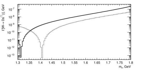
Figure 2: Dependence of the $W\to D_{s}\gamma$ decay widths on the quark masses in the NRQCD scheme. The charmed quark mass $m_{c}$ is plotted along the x-axis, the strange quark mass $m_{s}$ is calculated as $m_{s}=m_{D}-m_{c}$ or $m_{s}=m_{D^{*}}-m_{c}$. Solid curve, $W\to\gamma+D_{s}$; dotted curve, $W\to\gamma+{D_{s}}^{*}$.

On the other hand, one can argue that at the $W$ scale one should use the pole masses rather than constituent masses. Then, with setting $m_{c}=1.27$ GeV, $m_{s}=93.4$ MeV [16] (and rather unphysical $m_{D}=m_{c}+m_{s}$), we obtain

$$\Gamma(W\to D_{s}\gamma)=\Gamma(W\to D_{s}^{*}\gamma)=1.79\cdot 10^{-9}.$$ (34)

The sensitivity of the NRQCD results to the quark masses represents our first finding.

Now let us turn to the LC scheme. Given the fact that the meson energies are much larger than their masses, one can apparently use the massless approximation, as it is done in refs. [1, 3, 4]. However, taking the limit $m_{D}\to 0$ needs some care. The physical $D_{s}^{*}$ meson is not massless and may have longitudinal polarization. On the other hand, if we set the meson massless from the very beginning, we are unable to define its longitudinal polarization vector, and so, are unable to perform the relevant calculation. This was probably the reason for not showing the respective results in [3, 4].

In our real calculations we attribute some small but finite values to the quark masses (while keeping the relation $m_{c}+m_{s}=m_{D}$). By doing this, we obtain a numerically stable result which is fairly insensitive to the choice of quark masses and their ratios. Hereafter we will call this the small-mass limit. An important advantage of using finite (non-zero) masses is that we obtain a numerically stable result for the longitudinal polarization as well. The latter neither depends on the quark masses nor on the ratio $m_{s}/m_{c}$ and represents in our opinion a physically consistent description of real massive $D_{s}$ mesons. We emphasise that using the strict identity $m_{D}=0$ would lead to loosing an essential contribution.

In the small-mass limit, the decay width for the $D^{*}_{s}\gamma$ channel tends to a constant value equal to that for the $D_{s}\gamma$ channel. The crucial role of the longitudinal polarization is our second finding.

An important part of theoretical uncertainties in the LC scheme comes from the shape of the wave functions. The decay amplitudes (13) show peaks at $z=0$ and $z=1$, see Fig. 3. That means that the integral (31) is not dominated by the central part of the distribution $\Phi_{D}(z)$, but rather by its tails. As a consequence, the functions $\Phi_{D}(z)$ which look almost indistinguishable may lead to significantly different predictions for the decay widths. To illustrate the variability of theoretical predictions we tried the model parametrizations of the form

$$\Phi_{D}(z) \propto z^{a_{c}}\bar{z}^{a_{s}},$$ (35)

$$\Phi_{D}(z) \propto z^{a_{c}}\bar{z}^{a_{s}}\exp(-\bar{z}/\sigma),$$ (36)

where $\bar{z}=1-z$, and the respective results are collected in Table 3.1. We can conclude that the overall normalization of the wave function is much less important than its endpoint behavior. This fact constitutes our third finding.

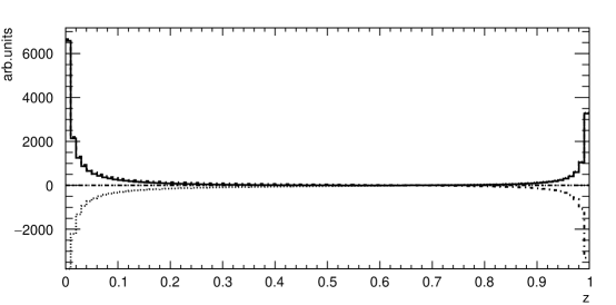
Figure 3: Upper panel: behavior of the $W\to D_{s}\gamma$ decay amplitudes as functions of the $c$-quark momentum fraction $z$ in the LC scheme. Dashed and dash-dotted curves represent different polarization states of the $W$ and the photon.
Lower panel: examples of different parametrizations of the $D_{s}$ wave function. Dotted curve, Equ. (36) with $a_{c}=3.1$, $a_{s}=1.2$; dashed curve, Equ. (35) with $a_{c}=0.9$, $a_{s}=1.1$, $\sigma=0.279$; dash-dotted curve, Equ. (35) with $a_{c}=1.1$, $a_{s}=0.9$, $\sigma=0.279$.

The difference between NRQCD and LC results streams from the fact that NRQCD probes the central region $z\simeq m_{c}/m_{D}$, while LC probes the endpoint regions $z\simeq 0$ and $z\simeq 1$, which have nothing in common. Summing up, the overall accuracy of theoretical predictions can hardly be made better than within one order of magnitude.

The $W\to D_{s}^{(*)}\gamma$ decay widths calculated for different parametrizations of the $D_{s}$ wave functions, eqs. (36), (35). Channel $a_{c}$ $a_{s}$ $\sigma$ $\Gamma_{W}$ Br [GeV] $W\to D_{s}^{(*)}\gamma$ 3.1 1.2 – $7.12{\cdot}10^{-9}$ $W\to D_{s}^{(*)}\gamma$ 1.0 1.0 0.279 $1.96{\cdot}10^{-8}$ $W\to D_{s}^{(*)}\gamma$ 1.1 0.9 0.279 $1.31{\cdot}10^{-8}$ $W\to D_{s}^{(*)}\gamma$ 0.9 1.1 0.279 $3.06{\cdot}10^{-8}$ $W\to D_{s}^{(*)}\gamma$ 1.0 1.0 0.280 $1.94{\cdot}10^{-8}$

Characteristics of the invariant mass distributions for $D_{s}^{(*)}+\gamma$ states produced in different $W$ decay modes.
Channel $\bar{m}(D_{s}\gamma)[GeV]$ r.m.s. [GeV] $\Gamma_{W}$ Br [GeV] $\Gamma_{W}$ Br [GeV] NRQCD LC $D_{s}+\gamma$ 80.386 1.042 $9.77{\cdot}10^{-9}$ $7.12{\cdot}10^{-9}$ $D_{s}^{*}+\gamma$ 77.749 1.837 $1.86{\cdot}10^{-9}$ $7.12{\cdot}10^{-9}$

3.2 Hadronic decays containing $J/\psi$

Hadronic decays of this kind may proceed both due to strong and electromagnetic interactions. The electromagnetic contribution is represented by the amplitudes (13) supplemented with a conversion of the photon into $J/\psi$ or $\psi(2S)$ meson (18). The strong contribution is represented by the amplitudes (14). Taken solely, the strong contribution shows almost no dependence on the quark masses. The behavior of the electromagnetic contribution has been discussed in the previous subsection.

Our major discovery concerning these decays is that the electromagnetic contribution is not negligible in comparison with the strong contribution, but even can take over. The relative suppression of the strong contribution comes from the intermediate gluon propagator.

The case when electromagnetic contributions are comparable with or even larger than strong contributions is rather rare, though not unique. A similar effect is present in the decays of Z-boson and H-bosons, see discussion in [21, 22, 23].

Our predictions for the NRQCD scheme are shown in Table 3.2. Shown there are the mass central value $\bar{m}(\psi\,D_{s})$; the dispersion (root of mean square); and the integral contribution to the $W$ width multiplied by the relevant branching fractions ($\psi^{\prime}\to J/\psi\,X,\;\chi_{c}\to J/\psi\,\gamma,\;D_{s}^{*}\to D_{s}\,X$). For the processes including photonic contributions (four entries in the bottom part of the Table 3.2) the quark mass setting was $m_{c}=m_{\psi}/2$=1.55 GeV, $m_{s}=m_{D^{(*)}}-m_{c}$. The exact $\psi(2S)$ mass was, however, taken into account in the amplitude conversion factor (18). For all other cases we set $m_{c}$ to one half of the quarkonium mass.

Characteristics of the invariant mass distributions for $J/\psi+D_{s}$ states produced in different $W$ decay modes; NRQCD predictions. Channel $\bar{m}(\psi{+}D_{s})$ [GeV] r.m.s. [GeV] $\Gamma_{W}$ Br [GeV]                    For strong contributions taken solely $J/\psi+D_{s}$ 80.35 1.04 $9.65{\cdot}10^{-12}$ $J/\psi+D_{s}^{*}$ 77.73 1.84 $9.74{\cdot}10^{-12}$ $\psi(2s)+D_{s}$ 73.75 2.63 $1.68{\cdot}10^{-12}$ $\psi(2s)+D_{s}^{*}$ 71.40 2.87 $1.67{\cdot}10^{-12}$ $\chi_{c0}+D_{s}$ 75.85 2.82 $1.96{\cdot}10^{-13}$ $\chi_{c1}+D_{s}$ 75.85 2.82 $4.27{\cdot}10^{-13}$ $\chi_{c2}+D_{s}$ 75.85 2.82 $8.08{\cdot}10^{-14}$ $\chi_{c0}+D_{s}^{*}$ 73.38 3.09 $2.43{\cdot}10^{-13}$ $\chi_{c1}+D_{s}^{*}$ 73.38 3.09 $4.25{\cdot}10^{-13}$ $\chi_{c2}+D_{s}^{*}$ 73.38 3.09 $8.09{\cdot}10^{-14}$ Strong and photonic contributions taken together including the interference $J/\psi+D_{s}$ $2.09{\cdot}10^{-11}$ $J/\psi+D_{s}^{*}$ $1.24{\cdot}10^{-11}$ $\psi(2s)+D_{s}$ $5.38{\cdot}10^{-12}$ $\psi(2s)+D_{s}^{*}$ $3.53{\cdot}10^{-12}$

The estimations based on the LC scheme are typically much higher than those based on NRQCD. This is a consequence of the pole in the gluon propagator in (14). This divergence strongly emphasises the region of small quark momentum fractions (see Fig. 4) and makes the predictions very sensitive to the endpoint behavior of the mesons’ wave functions. Using the parametrizations proposed in Ref. [1]

$$\Phi_{D}(z_{c}) \propto (z_{c})^{3.1}(z_{\bar{s}})^{1.2},$$

$$\Phi_{\psi}(z_{c}) \propto z_{c}z_{\bar{c}}\,\exp\{-0.95/(z_{c}z_{\bar{c}})\}$$ (37)

with $z_{\bar{s}}=1{-}z_{c}$ and $z_{\bar{c}}=1{-}z_{c}$ we obtain

$$\Gamma(W\to J\psi D_{s})=3.28{\cdot}10^{-11}$$ (38)

$$\Gamma(W\to J\psi D_{s}^{*})=3.85{\cdot}10^{-11}$$ (39)

In Table 3.2 we show that the parametrizations of $\Phi_{D}(z_{1})$ and $\Phi_{J/\psi}(z_{2})$ may lead to noticeably different predictions for the decay widths. The distribution amplitudes of $D_{s}^{(*)}$ mesons are taken according to eqs. (35) and (36), and those of the $J/\psi$ meson are taken in the form

$$\Phi_{\psi}(z) \propto z^{b_{c}}\bar{z}^{b_{s}}\exp\{-(\bar{z}-0.5)^{2}/\sigma_{2}\},$$ (40)

$$\Phi_{\psi}(z) \propto z^{b_{c}}\bar{z}^{b_{s}}\exp\{-0.95/(z\bar{z})\},$$ (41)

These expressions represent simple low-scale ($\mu^{2}\simeq m_{\psi}^{2}$) parametrizations of $\Phi(z)$, and our calculations reveal large numerical uncertainties already at that scale. We use these toy parametrizations for illustrative purposes, without evolving them to a higher scale $\mu^{2}\simeq m_{W}^{2}$, because the goal of our study is not in producing ’exact’ predictions (a task not looking feasible in full sense), but rather in giving an estimate of the overall uncertainty.

We do expect large corrections from Efremov-Radyushkin-Brodsky-Lepage (ERBL) evolution which can significantly change the behavior of $\Phi(z)$ at $z$ close to 0. At the same time, the evolution in its turn brings additional uncertainties connected to the accuracy of the ERBL equation at $z\simeq 0$.

We also have to note that the importance of small-$z$ region (which is the region of zero quark momentum) opens a room for final state interactions. The latter can hardly be described in a reliable way and make all theoretical predictions even more uncertain.

Channel	$a_{c}$	$a_{s}$	$\sigma_{1}$	$b_{c}$	$b_{s}$	$\sigma_{2}$	$\Gamma_{W}$ Br [GeV]
$J/\psi+D_{s}$	3.1	1.2	–	1.0	1.0	–	$3.28{\cdot}10^{-11}$
$J/\psi+D_{s}$	1.0	1.0	0.279	1.1	0.9	0.234	$6.31{\cdot}10^{-11}$
$J/\psi+D_{s}$	1.1	0.9	0.279	1.0	1.0	0.234	$5.53{\cdot}10^{-11}$
$J/\psi+D_{s}^{*}$	3.1	1.2	–	1.0	1.0	–	$3.85{\cdot}10^{-11}$
$J/\psi+D_{s}^{*}$	1.0	1.0	0.279	1.1	0.9	0.234	$8.44{\cdot}10^{-11}$
$J/\psi+D_{s}^{*}$	1.1	0.9	0.279	1.0	1.0	0.234	$7.33{\cdot}10^{-11}$

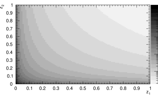
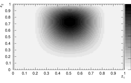
Figure 4: Upper panel: behavior of the gluon propagator as a function of the $\bar{c}$-quarks’ momentum fractions $z_{1}$ and $z_{2}$ in the LC scheme. The polarization states of the $W$ and the $J/\psi$ are longitudinal. Note the logarithm scale. Lower panel: behavior of the convolution of $J/\psi$ and $D_{s}$ wave functions.

3.3 Hadronic decays not containing $J/\psi$

The channels which do not contain $J/\psi$ meson as an immediate product may still have it in the final state due to secondary decays:  $\psi^{\prime}\to J/\psi\,\pi\,\pi$,  $\chi_{c}\to J/\psi\,\gamma$  $D_{s}^{*}\to D_{s}\,\pi^{0}$,  $D_{s}^{*}\to D_{s}\,\gamma$. The whole group of the decay modes (3)-(8) ends up with the $J/\psi+D_{s}$ combination, but with distorted invariant mass distribution.

Fig. 5 displays the invariant mass distributions for $J/\psi\,D_{s}$ states produced through different $W$ decay modes. The contributions (3) and (4) overlap and cannot be resolved into individual peaks. This makes the experimental analysis more complicated and would require a multiparametric (probably, double-gaussian) fit to describe the signal. The other contributions (5)-(8) are separable from the ’main’ peak and can be rejected by simple kinematic constraints.

In Table 3.3, we show our results for $b$-flavored modes (9)-(12). The formation of $b$-flavored mesons shows somewhat larger probability (because of larger values of the wave functions), but these modes may be less convenient from the point of view of meson identification.

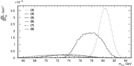
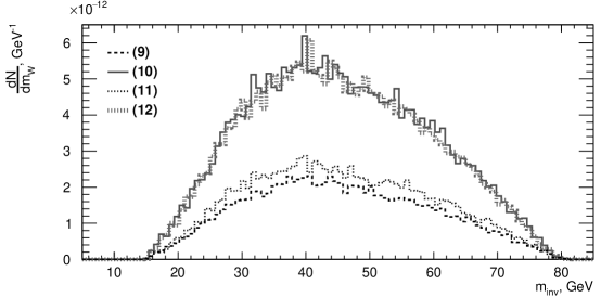
Figure 5: The invariant mass distributions for $J/\psi$ +$D_{s}$ states for different $W$ decay modes. Upper panel: processes (3) - (8) Lower panel: processes (9) - (12).

NRQCD predictions. $\bar{m}(B_{c}{+}B_{s})$ [GeV] r.m.s. [GeV] $\Gamma_{W}$ Br [GeV] Channel $B_{c}+B_{s}$ 45.49 13.89 $5.26{\cdot}10^{-12}$ $B_{c}+B_{s}^{*}$ 45.33 13.77 $5.73{\cdot}10^{-12}$ $B_{c}^{*}+B_{s}$ 45.41 13.78 $4.11{\cdot}10^{-12}$ $B_{c}^{*}+B_{s}^{*}$ 45.27 13.77 $5.55{\cdot}10^{-12}$

4 Conclusions

We have analyzed several exclusive two-body decays of $W$ and reached the following conclusions:

– In the NRQCD scheme, the predictions are highly sensitive to the quark mass definition.

– In the LC scheme, the predictions are primarily impacted by the behavior of the meson wave function at $z=0$ and $z=1$, with little significance given to its central value. This makes the theoretical predictions less certain than it was previously believed, because of both poorly known behavior of meson wave functions at the endpoints and the potentially non-negligible role of final state interactions.

– The longitudinal polarization of vector mesons dominates the respective W decays, resulting in decay widths equal to those found for pseudoscalar mesons.

Our analysis of the hadronic mode $J/\psi+D_{s}^{(*)}$ shows that the conclusions derived for the meson-photonic decay modes also hold true. A noteworthy finding is that the electromagnetic contributions to these decays are substantial, and may even surpass the strong contributions.

We also revealed that the secondary decays have a notable impact, leading to overlapping invariant mass distributions for $J/\psi,D_{s}$ and $J/\psi,D_{s}^{*}$ modes. To accurately describe the signal, a multiparametric fitting function is required. The mass distributions for other modes, however, are distinct and separable through kinematic constraints.

The $W$ decay modes involving $b$-flavored mesons exhibit larger branching fractions compared to the $c$-flavored modes. However, the challenge lies in accurately identifying the final mesons in these decays.

Our analysis maintains the previous conclusion  that the W decay branching fractions into $J/\psi,D_{s}^{(*)}$ and $D_{s}^{(*)},\gamma$ are still too small to warrant experimental detection with current sensitivity established at the level $6.5\cdot 10^{-4}$ [19]. The inclusion of new important contributions does not change this conclusion.

Acknowledgments

Alexander Sakharov thanks Prof. Robert Harr from Wayne State University for initiating fruitful discussions on the topic of the study. The work of Alsu Bagdatova and Sergey Baranov was supported by the Russian Science Foundation under Grant No. 22-22-00119.

References

• [1] A.V. Luchinsky and A.K. Likhoded, Mod. Phys. Lett. A 36 (2021) 2150058. DOI: 10.1142/S0217732321500589.
• [2] U. Baur, CERN-TH.50688, MAD/PH/412; U. Baur and L. Berger, Phys. Rev. D 41 (1990) 1476, DOI:10.1103/Phys. Rev. D . (1.1476.) 4
• [3] L. Arnellos, W.J.Marciano, and Z. Parsa, Nucl. Phys. B 196 (1982) 378.
• [4] Y. Grossman, M. KΓΆnig, and M. Neubert, JHEP 1504 (2015) 101.
• [5] C.-H. Chang, Nucl. Phys. B172 (1980) 425.
• [6] E.L. Berger and D. Jones, Phys. Rev. D 23 (1981) 1521.
• [7] R. Baier and R. RΓΌckl, Phys. Lett. B 102 (1981) 364.
• [8] H. Krasemann, Zeit. Phys. C 1 (1979) 189;
• [9] G. Guberina, J. KΓΌhn, R. Peccei, and R. RΓΌckl, Nucl. Phys. B174 (1980) 317.
• [10] M. Mangano and T. Melia, arXiv:1410.7475 [hep-ph].
• [11] J.A.M. Vermaseren, Symbolic Manipulations with FORM, published by CAN (Computer Algebra Nederland), Kruislaan 413, 1098, SJ Amsterdaam, 1991, ISBN 90-74116-01-9.
• [12] E. Bycling, K. Kajantie, Particle Kinematics, published by John Wiley and Sons, New York, 1973.
• [13] V.L. Chernyak and A.R. Zhitnitsky, Phys. Rep. 112 (1984) 173.
• [14] E.J. Eichten and C. Quigg, Phys. Rev. D 52 (1995) 1726.
• [15] E.J. Eichten and C. Quigg, arXiv:1904.11542 [hep-ph] .
• [16] R.L. Workman et al., Particle Data Group, Prog. Theor. Exp. Phys. 2022 (2022) 083C01.
• [17] D. Hwang and Y.-Y. Keum, Phys. Rev. D 61 (2000) 073003. DOI:10.1103/PhysRevD.61.073003, https://arxiv.org/pdf/hep-ph/9905433.pdf
• [18] R. Balasubramanian and B. Blossier, Eur. Phys. J. C 80 (2020) 412. DOI:10.1140/epjc/s10052-020-7965-z, https://arxiv.org/pdf/1912.09937.pdf
• [19] [LHCb], [arXiv:2212.07120 [hep-ex]].
• [20] Eric Braaten, Kingman Cheung, Sean Fleming, Tzu Chiang Yuan,Phys. Rev. D 51 (1995.) 4819DOI:10.1103/PhysRevD.51.4819 https://doi.org/10.48550/arXiv.hep-ph/9409316
• [21] Dao-Neng Gao, Xi Gong, Phys. Lett. B 832 (2022) 137243. DOI:10.1016/j.physletb.2022.137243.
• [22] I.N. Belov, A.V. Berezhnoy, E.A. Leshchenko, Symmetry 2021, 13(7), 1262; DOI:10.3390/sym13071262
• [23] I.N. Belov, A.V. Berezhnoy, E.A. Leshchenko https://doi.org/10.48550/arXiv.2303.03362