One-loop calculations in the chirality-flow formalism

Abstract

In a few recent papers we introduced the chirality-flow formalism, which was shown to make calculations of tree-level Feynman diagrams simple and transparent. Chirality flow, which is based on the spinor-helicity formalism, allows to often immediately analytically write down a tree-level Feynman diagram in terms of spinor inner products. In this paper, we argue that there is also a significant simplification of the Lorentz structure at the one-loop level, at least when using the four-dimensional formulation of the four-dimensional helicity scheme. Additionally, we find that the possible terms in a tensor decomposition of loop integrals are highly constrained, and therefore the tensor reduction procedure is simplified.

1 Introduction

In a few recent papers we introduced the chirality-flow formalism Lifson:2020pai ; Alnefjord:2020xqr ; Lifson:2022ijv ; Platzer:2022nfu . This graphical method builds on the spinor-helicity formalism DeCausmaecker:1981jtq ; Berends:1981rb ; Berends:1981uq ; DeCausmaecker:1981wzb ; Berends:1983ez ; Farrar:1983wk ; Kleiss:1984dp ; Berends:1984gf ; Gunion:1985bp ; Gunion:1985vca ; Kleiss:1985yh ; Hagiwara:1985yu ; Kleiss:1986ct ; Kleiss:1986qc ; Xu:1986xb ; Dittmaier:1998nn ; Schwinn:2005pi ; Dixon:1996wi ; Elvang:2013cua , and relies on splitting the Lorentz algebra into left- and right-chiral parts. As for the spinor-helicity formalism, all objects, in particular polarization vectors, are rewritten in terms of massless spinors, but the chirality-flow method takes the simplification one step further by recasting everything into diagrammatic “flows”, i.e., contractions of spinors.

This allows for rewriting Feynman rules and diagrams directly in terms of these flows and invariants, and results in amplitudes that may be directly expressed in terms of spinor inner products, i.e., the only Lorentz invariant quantities at hand Lifson:2020pai ; Alnefjord:2020xqr . Methods which are able to directly decompose amplitudes in terms of the available group and spinor structures are of utmost importance to provide reliable input to resummation approaches at the amplitude level Forshaw:2019ver ; DeAngelis:2020rvq ; Platzer:2020lbr ; Platzer:2022nfu ; Platzer:2022jny .

For tree-level calculations, the chirality-flow formalism leads to significant simplifications Lifson:2020pai ; Alnefjord:2020xqr . In practice, it is often possible to immediately write down the amplitude corresponding to a Feynman diagram. On top of this, reference vectors for external gauge bosons or spin directions can be chosen in such a way that many Feynman diagrams simplify or vanish. This — as well as the simplified algebra — led to a significant speed-up for a tree-level test implementation in MadGraph5_aMC@NLO Lifson:2022ijv .

Moving beyond tree-level, it is imperative to use a consistent regularization scheme, which requires a careful treatment of chirality and $\gamma^{5}$ tHooft:1972tcz ; Breitenlohner:1977hr ; Jones:1982zf ; Korner:1991sx ; Kreimer:1993bh ; Larin:1993tq ; Trueman:1995ca ; Jegerlehner:2000dz ; Tsai:2009hp ; Tsai:2009it ; Ferrari:2014jqa ; Ferrari:2015mha ; Ferrari:2016nea ; Viglioni:2016nqc ; Gnendiger:2017rfh ; Bruque:2018bmy ; Belusca-Maito:2022usw . A comprehensive summary of different regularization methods can be found in Gnendiger:2017pys ; Heinrich:2020ybq . In conventional dimensional regularization (CDR) Bollini:1972ui ; tHooft:1972tcz ; Breitenlohner:1977hr , all objects are regularized in $d$ dimensions, which (at least naively) would destroy many of the simplifications brought about by chirality flow. While in the long term we aim at a full treatment of chirality flow in CDR (such as to use chirality flow to extract $\epsilon$-dependent quantities in tree-level calculations), in the present paper we instead exploit a (partially) four-dimensional regularization scheme, the 4$d$ formulation (FDF) Fazio:2014xea of the 4$d$ helicity scheme (FDH) Bern:1991aq ; Bern:2002tk , in order to retain the significant simplifications which chirality flow draws from using charge conjugations, Fierz and possibly Schouten identities. In FDF, loop numerators are written as purely four-dimensional objects together with some additional Lorentz scalars, while the loop momenta and integrals are in $d$ dimensions. This implies that the algebraic manipulations implemented for tree-level calculations in four dimensions Lifson:2020pai ; Alnefjord:2020xqr can be retained, and Feynman diagrams are therefore easily “flowable” — as in tree-level calculations. After using chirality flow to simplify the Lorentz algebra, the integrals are in $d$ dimensions, so we are able to use all of the standard properties and results of dimensionally regularized integrals.

The rest of this paper is organized as follows. In section 2, we give a brief introduction to chirality flow and how it is used in Feynman-diagram-based amplitude calculations. Then, the 4$d$ formulation of the 4$d$ helicity scheme is introduced in section 3. In section 4, we illustrate with a few examples how to do one-loop calculations in chirality flow, describing how chirality flow simplifies the Lorentz algebra and tensor reduction. Finally, we conclude in section 5.

2 Introduction to chirality flow

In this section, we give a brief introduction to the chirality-flow formalism, and exemplify how spinors, propagators and vertices are defined. A complete list of standard model external wave functions, vertices and propagators can be found in Alnefjord:2020xqr , whereas all structures needed for this paper are contained either in the main text or in appendix A. For details of conventions, we refer the reader to Lifson:2020pai .

The basic building blocks of the chirality-flow formalism are the left- and right-chiral spinors, which we represent graphically in terms of dotted and undotted lines respectively Lifson:2020pai ,

$${\color[rgb]{1,0,0}\langle}i{\color[rgb]{1,0,0}|} =\raisebox{-0.3pt}{\includegraphics[scale={0.4}]{Jaxodraw/MS/ExtSpinorSolidiCol}},\qquad{\color[rgb]{0,0,1}[}i{\color[rgb]{0,0,1}|} =\raisebox{-0.3pt}{\includegraphics[scale={0.4}]{Jaxodraw/MS/ExtSpinorDottediCol}},$$

$${\color[rgb]{1,0,0}|}j{\color[rgb]{1,0,0}\rangle} =\raisebox{-0.3pt}{\includegraphics[scale={0.4}]{Jaxodraw/MS/ExtSpinorSolidjCol}},\qquad{\color[rgb]{0,0,1}|}j{\color[rgb]{0,0,1}]} =\raisebox{-0.3pt}{\includegraphics[scale={0.4}]{Jaxodraw/MS/ExtSpinorDottedjCol}},$$ (2.0.1)

with ${\color[rgb]{1,0,0}\langle}i{\color[rgb]{1,0,0}|}={\color[rgb]{1,0,0}\langle}p_{i}{\color[rgb]{1,0,0}|}$ etc. We represent contractions of these spinors with “flows”

$${\color[rgb]{1,0,0}\langle}ij{\color[rgb]{1,0,0}\rangle}\equiv\epsilon^{\alpha\beta}\lambda_{i,\beta}\lambda_{j,\alpha}={\includegraphics[scale={0.4}]{Jaxodraw/MS/SpinorProdAngleijCol}}~{},\;\;\;{\color[rgb]{0,0,1}[}ij{\color[rgb]{0,0,1}]}\equiv\epsilon_{{\dot{\alpha}}{\dot{\beta}}}\tilde{\lambda}_{i}^{{\dot{\beta}}}\tilde{\lambda}_{j}^{{\dot{\alpha}}}=\raisebox{-0.2pt}{\includegraphics[scale={0.4}]{Jaxodraw/MS/SpinorProdSquareijCol}}~{},$$ (2.0.2)

where (up to a phase) ${\color[rgb]{1,0,0}\langle}ij{\color[rgb]{1,0,0}\rangle}\sim{\color[rgb]{0,0,1}[}ij{\color[rgb]{0,0,1}]}\sim\sqrt{2p_{i}\cdot p_{j}}$, and where the antisymmetry of the spinor inner product is obvious. We read chirality-flow lines along the chirality-flow arrow, and, because the inner product is antisymmetric, swapping the chirality-flow arrow direction induces a minus sign.

All particles and momenta are then written as (a combination of) massless spinors. For example, massless polarization vectors are given by

$$\epsilon_{\color[rgb]{0,0,1}{L}}(p_{i},r) =\frac{1}{{\color[rgb]{1,0,0}\langle}ri{\color[rgb]{1,0,0}\rangle}}\raisebox{-0.2pt}{\includegraphics[scale={0.35}]{Jaxodraw/MS/PhotonExtFlowPlaRevCol}}\quad\text{or}\quad\,\,\frac{1}{{\color[rgb]{1,0,0}\langle}ri{\color[rgb]{1,0,0}\rangle}}\raisebox{-0.2pt}{\includegraphics[scale={0.35}]{Jaxodraw/MS/PhotonExtFlowPlaCol}},$$

$$\epsilon_{\color[rgb]{1,0,0}{R}}(p_{i},r) =\frac{1}{{\color[rgb]{0,0,1}[}ir{\color[rgb]{0,0,1}]}}\raisebox{-0.2pt}{\includegraphics[scale={0.35}]{Jaxodraw/MS/PhotonExtFlowMiaCol}}\quad\,\,\text{or}\quad\,\,\frac{1}{{\color[rgb]{0,0,1}[}ir{\color[rgb]{0,0,1}]}}\raisebox{-0.2pt}{\includegraphics[scale={0.35}]{Jaxodraw/MS/PhotonExtFlowMiaRevCol}},$$ (2.0.3)

where, similar to chiral spinors, we label the polarization vectors $\color[rgb]{0,0,1}{L}/\color[rgb]{1,0,0}{R}$ for convenience, with $\epsilon_{\color[rgb]{0,0,1}{L}}(p_{i},r)$ denoting a negative-helicity incoming or positive-helicity outgoing photon of momentum $p_{i}$, and $\epsilon_{\color[rgb]{1,0,0}{R}}(p_{i},r)$ denoting a positive-helicity incoming or negative-helicity outgoing photon. Here, $r$ is an arbitrary (massless) reference vector with $r\cdot p_{i}\neq 0$, and either set of opposing arrow directions may be used as long as it matches the rest of the diagram Lifson:2020pai .

To describe massive particles and momenta, a massive momentum $p$ with $p^{2}=m^{2}\neq 0$ is decomposed into a sum of massless momenta $p^{\flat}$ and $q$ as

$$p^{\mu}=p^{\flat,\mu}+\alpha q^{\mu}~{},\qquad(p^{\flat})^{2}=q^{2}=0,\qquad p^{2}=m^{2}~{},\qquad\alpha=\frac{m^{2}}{2p^{\flat}\cdot q}=\frac{m^{2}}{2p\cdot q}~{},$$ (2.0.4)

with, for example, an incoming spinor with spin along the axis $s^{\mu}=(p^{\mu}-2\alpha q^{\mu})/m$ given by Alnefjord:2020xqr

$$u^{+}(p)=\begin{pmatrix}\frac{m}{{\color[rgb]{0,0,1}[}p^{\flat}q{\color[rgb]{0,0,1}]}}\raisebox{-0.2pt}{\includegraphics[scale={0.40}]{Jaxodraw/MS/ExtSpinorAntiDotted_qCol}}\\ \phantom{\frac{m}{{\color[rgb]{0,0,1}[}p^{\flat}q{\color[rgb]{0,0,1}]}}}\raisebox{-0.2pt}{\includegraphics[scale={0.40}]{Jaxodraw/MS/ExtSpinorAntiSolid_pflatCol}}\end{pmatrix}\;.$$ (2.0.5)

While it is natural in chirality flow to measure spin along any direction, we can of course also measure it along the direction of motion, in which case we choose $\alpha=1$, $q^{\mu}=p_{b}^{\mu}$ and $p^{\flat,\mu}=p_{f}^{\mu}$, with $\vec{p}_{f}$ pointing in the same direction as $\vec{p}$ and $\vec{p}_{b}$ pointing in the opposite direction, i.e.,

$$p_{f}^{\mu} =\frac{p^{0}+|\vec{p}|}{2}\big{(}1,\hat{p}\big{)}~{}, p_{b}^{\mu} =\frac{p^{0}-|\vec{p}|}{2}\big{(}1,-\hat{p}\big{)}~{},$$ (2.0.6)

such that the three-vector of the spin $s^{\mu}=\frac{1}{m}(p_{f}^{\mu}-p_{b}^{\mu})=\frac{1}{m}(|\vec{p}|,p^{0}\hat{p})$, is directed along the motion, giving the helicity basis,

$$u^{+}(p) =\begin{pmatrix}\frac{m}{{\color[rgb]{0,0,1}[}p_{f}p_{b}{\color[rgb]{0,0,1}]}}\raisebox{-5.5pt}{\includegraphics[scale={0.375}]{./Jaxodraw/MS/ExtSpinorAntiDotted_pbCol}}\\ \phantom{\frac{m}{{\color[rgb]{0,0,1}[}p_{f}p_{b}{\color[rgb]{0,0,1}]}}}\raisebox{-5.5pt}{\includegraphics[scale={0.375}]{./Jaxodraw/MS/ExtSpinorAntiSolid_pfCol}}\end{pmatrix}\stackrel{{\scriptstyle\hbox{$m\rightarrow 0$}}}{{\hbox{$\longrightarrow$}}}\begin{pmatrix}0\\ \raisebox{-5.5pt}{\includegraphics[scale={0.375}]{./Jaxodraw/MS/ExtSpinorAntiSolid_pCol}}\end{pmatrix}\;.$$ (2.0.7)

Vertices and propagators are also naturally described using chirality flow. For example, the QED vertex can be translated to

$$\includegraphics[scale={0.45},valign={c}]{Jaxodraw/fPhotonVertexMassless}\!\!\!\!\!=ieQ_{f}\gamma^{\mu} =ieQ_{f}\begin{pmatrix}0&\sqrt{2}\tau^{\mu,{\dot{\alpha}}\beta}\\ \sqrt{2}\bar{\tau}^{\mu}_{\alpha{\dot{\beta}}}&0\end{pmatrix}$$

$$=ieQ_{f}\sqrt{2}\begin{pmatrix}0&\raisebox{-0.35pt}{\includegraphics[scale={0.35}]{Jaxodraw/FermionVectorVertexR}}\\ \raisebox{-0.4pt}{\includegraphics[scale={0.385}]{./Jaxodraw/FermionVectorVertexL}}&0\end{pmatrix}~{},$$ (2.0.8)

where we introduce our differently-normalized Pauli matrices $\tau^{\mu}\equiv\sigma^{\mu}/\sqrt{2}$ and $\bar{\tau}^{\mu}\equiv\bar{\sigma}^{\mu}/\sqrt{2}$, and our use of the chiral basis is made explicit. The propagator for a massless gauge boson in the Feynman gauge contains the chirality-flow rule for the metric, which is a double line with arrows opposing,

$$=\quad-i\frac{g_{\mu\nu}}{p^{2}} \rightarrow -\frac{i}{p^{2}}\raisebox{-0.25pt}{\includegraphics[scale={0.45}]{Jaxodraw/PhotonPropFlowa}} -\frac{i}{p^{2}}\raisebox{-0.25pt}{\includegraphics[scale={0.45}]{Jaxodraw/PhotonPropFlowb}}\;,$$ or (2.0.9)

while the fermion propagator in the flow picture is

$$=\ \frac{i}{p^{2}-m^{2}}\begin{pmatrix}m{\delta^{{\dot{\alpha}}}}_{{\dot{\beta}}}&\sqrt{2}p^{{\dot{\alpha}}\beta}\\ \sqrt{2}\bar{p}_{\alpha{\dot{\beta}}}&m{\delta_{\alpha}}^{\beta}\end{pmatrix}=\frac{i}{p^{2}-m^{2}}\begin{pmatrix}m\includegraphics[scale={0.34}]{Jaxodraw/MS/KroneckerDeltaDottedPropCol}&\includegraphics[scale={0.34}]{Jaxodraw/MS/FermionPropFlowDottedSolodAlphaBetaCol}\\ \includegraphics[scale={0.34}]{Jaxodraw/MS/FermionPropFlowSolidDottedAlphaBetaCol}&m\includegraphics[scale={0.34}]{Jaxodraw/MS/KroneckerDeltaUndottedCol}\end{pmatrix}\;,$$ (2.0.10)

where we have introduced a graphical “momentum-dot” notation for momenta slashed with $\sigma$ or $\bar{\sigma}$. Note that any momentum in the Feynman rules will be translated to this momentum-dot in the chirality-flow rules using

$$p^{\mu} \rightarrow\frac{1}{\sqrt{2}}\raisebox{-0.15pt}{\includegraphics[scale={0.4}]{./Jaxodraw/MS/FermionPropFlowDottedSolidpCol}}~{}, p^{\mu} \rightarrow\frac{1}{\sqrt{2}}\raisebox{-0.15pt}{\includegraphics[scale={0.4}]{./Jaxodraw/MS/FermionPropFlowSolidDottedpCol}}~{},$$ or (2.0.11)

where, like with the polarization vectors in eq. (2.0.3), either arrow direction in eqs. (2.0.9) and (2.0.11) is allowed as long as it matches the rest of the diagram Lifson:2020pai .

Using these rules, it is easy to immediately write down the values of Feynman diagrams, for example, in massless QED,

(2.0.15)

$$\times{{\color[rgb]{0,0,1}[15]}}{{\color[rgb]{1,0,0}\langle 64\rangle}}{{\color[rgb]{0,0.80078125,1}[10\,\,r_{9}]}}{{\color[rgb]{1,0.3984375,0}\Bigg{(}\underbrace{\langle 99\rangle}_{0}[9r_{8}]+\langle 9\,10\rangle[10\,r_{8}]\Bigg{)}}}{{\color[rgb]{0.3984375,0,0.99609375}\Bigg{(}\underbrace{[33]}_{0}\langle 37\rangle+[34]\langle 47\rangle+[36]\langle 67\rangle\Bigg{)}}}$$

$$\times{{\color[rgb]{0,0.80078125,0}\Big{(}-\langle 89\rangle[91]\langle 12\rangle-\langle 89\rangle[95]\langle 52\rangle-\langle 8\,10\rangle[10\,\,1]\langle 12\rangle-\langle 8\,10\rangle[10\,\,5]\langle 52\rangle\Big{)}}}\;,$$ (2.0.16)

where we have superimposed a chirality-flow diagram onto a ten-point Feynman diagram. For massless QED and QCD, any chirality-flow arrow direction which has opposing arrows for bosons and which flows through momentum-dots is equivalent Lifson:2020pai . If masses or scalar particles are involved, then some care is needed to set consistent arrow directions Alnefjord:2020xqr .

Finally, we also note that diagrams can be made to vanish by appropriately choosing the reference vectors of our polarization vectors and massive spinors. For example, the above diagram vanishes if we pick $r_{9}=10$.

In this paper, we will argue that much of the simplification from chirality flow can be retained at one-loop level. For example, we may simplify the algebra of the electron self-energy in Feynman gauge as

$$\raisebox{-0.4pt}{\includegraphics[scale={0.3}]{Jaxodraw/fermionSelfEnergyPhotonLRChiFlow}}\quad\sim\quad\raisebox{-0.4pt}{\includegraphics[scale={0.3}]{Jaxodraw/fermionSelfEnergyFlowLRNoArrows}}\;,$$ (2.0.17)

where we defer a discussion on the arrow direction until section 4. The diagrammatic identity above is of course simple, but we will demonstrate that similar diagrammatic decompositions can be used together with certain methods of decomposing tensor integrals, and thereby significantly simplify calculations.

3 FDF

In this section we summarize the FDF formalism. This formalism was created in 2014 with the aim of providing a truly 4d numerator algebra for loop integrals. It has also been used in the context of color-kinematics duality Mastrolia:2015maa ; Primo:2016omk , while some example calculations in FDF can be found in Gnendiger:2017pys ; Gnendiger:2017rfh . Since the chirality-flow formalism makes use of explicitly 4d relations, the FDF method is easily converted into a flow formalism (though we expect that a similar flow formalism holds in CDR).

In FDF we have five vector spaces, the standard Minkowski space $S_{[4]}$ with four integer dimensions, and the infinite-dimensional spaces $QS_{[d]}$, $QS_{[d_{s}]}$, $QS_{[-2\epsilon]}$, $QS_{[n_{\epsilon}]}$, and $QS_{[n_{\epsilon}-2\epsilon]}$, which satisfy Fazio:2014xea

$$S_{[4]} \subset QS_{[d]}\subset QS_{[d_{s}]}~{}, QS_{[d]} =S_{[4]}\oplus QS_{[-2\epsilon]}~{},$$

$$QS_{[n_{\epsilon}-2\epsilon]} =QS_{[-2\epsilon]}\oplus QS_{[n_{\epsilon}]}~{}, QS_{[d_{s}]} =QS_{[d]}\oplus QS_{[n_{\epsilon}]}~{},$$ (3.0.1)

where $QS_{[d]}$ is the vector space of CDR, $QS_{[d_{s}]}$ with $d_{s}=4$ is the vector space of FDH and FDF, and we follow the notation of Gnendiger:2017pys ; Anger:2018ove . Since the subspaces in eq. (3.0.1) are orthogonal, we can split up vectors and tensors as e.g.

$$\gamma^{\mu}_{[d_{s}]} =\gamma^{\mu}_{[4]}+\gamma^{\mu}_{[n_{\epsilon}-2\epsilon]}~{}, g^{\mu\nu}_{[d_{s}]} =g^{\mu\nu}_{[4]}+g^{\mu\nu}_{[n_{\epsilon}-2\epsilon]}~{},$$ (3.0.2)

where the subscript in square brackets gives the vector space of the object. The metric is used to project onto the different subspaces, for example,

$$g^{\mu\nu}_{[d_{s}]}g_{\nu\rho[4]} =\delta^{\mu}_{\rho[4]}~{}, g^{\mu\nu}_{[d_{s}]}g_{\nu\rho[d]} =\delta^{\mu}_{\rho[d]}~{},$$ (3.0.3)

while the trace of the metric is given by the dimension of its (sub)space, and the Dirac gamma matrices have their usual anticommutation relations

$$(g_{[dim]})^{\mu}_{~{}\mu} =dim~{}, \left\{\gamma^{\mu}_{[dim]},\gamma^{\nu}_{[dim]}\right\} =2g^{\mu\nu}_{[dim]}~{}.$$ (3.0.4)

The main starting point of FDF is to re-write $QS_{[d_{s}]}$ as

$$QS_{[d_{s}]}=S_{[4]}\oplus QS_{[-2\epsilon]}\oplus QS_{[n_{\epsilon}]}=S_{[4]}\oplus QS_{[n_{\epsilon}-2\epsilon]}~{},$$ (3.0.5)

that is, as the purely 4d Minkowski space plus an extra space $QS_{[n_{\epsilon}-2\epsilon]}$ which can be represented by 4d objects multiplying a new algebra called the $-2\epsilon$ selection rules ($-2\epsilon$-SRs). The $-2\epsilon$-SRs are defined using the following replacements

$$g^{\mu\nu}_{[n_{\epsilon}-2\epsilon]} \rightarrow G^{MN}~{}, l_{[-2\epsilon]}^{\mu} \rightarrow i\mu Q^{M}~{}, \gamma^{\mu}_{[n_{\epsilon}-2\epsilon]} \rightarrow\gamma^{5}\Gamma^{M}~{},$$ (3.0.6)

together with the following algebra

$$G^{MN}G^{NP} =G^{MP}~{}, G^{MM} =0~{}, G^{MN} =G^{NM}~{},$$

$$\Gamma^{M}G^{MN} =\Gamma^{M}~{}, \Gamma^{M}\Gamma^{M} =0~{}, Q^{M}\Gamma^{M} =1~{},$$

$$Q^{M}G^{MN} =Q^{M}~{}, Q^{M}Q^{M} =1~{}, \left\{\Gamma^{M},\Gamma^{N}\right\} =2G^{MN}~{}.$$ (3.0.7)

In any given Feynman diagram the $-2\epsilon$-SRs can be precalculated, and contribute an overall multiplicative factor of $0$ or $\pm 1$ to the diagram.

In the Feynman rules of FDF, the $-2\epsilon$-SRs imply that fermion propagators within loops are rewritten to contain only 4d terms and a new mass $\mu$ Fazio:2014xea

$$\raisebox{-0.1pt}{\includegraphics[scale={0.4}]{./Jaxodraw/FermionProp}}\sim\ \not{l}_{[d_{s}]}+m =\not{l}_{[4]}+i\mu\gamma^{5}+m$$

$$=\begin{pmatrix}(m-i\mu)\includegraphics[scale={0.34}]{Jaxodraw/MS/KroneckerDeltaDottedPropColNoIndices}\;\;\;\;\;\;&\phantom{(m-i\mu)}\includegraphics[scale={0.34}]{Jaxodraw/MS/FermionPropFlowDottedSolidlCol}\\ \phantom{(m+i\mu)}\includegraphics[scale={0.34}]{Jaxodraw/MS/FermionPropFlowSolidDottedlCol}\;\;\;\;\;\;&(m+i\mu)\includegraphics[scale={0.34}]{Jaxodraw/MS/KroneckerDeltaUndottedColNoIndices}\end{pmatrix}~{},$$ (3.0.8)

and that vector boson propagators are split into two pieces, with numerator structure

$$\raisebox{-0.25pt}{\includegraphics[scale={0.4}]{Jaxodraw/PhotonProp}}\!\!\sim\ -ig^{\mu\nu}_{[d_{s}]}=-ig^{\mu\nu}_{[4]}-iG^{MN}=-i\raisebox{-0.25pt}{\includegraphics[scale={0.45}]{Jaxodraw/PhotonPropFlowNoArrows}}-iG^{MN}~{},$$ (3.0.9)

in Feynman gauge. Here, the first term is the usual 4d propagator with suppressed chirality-flow arrows (recall that these arrows should be opposing, see section 2), and the second is called an FDF scalar and has trivial Lorentz structure.

To build the correct Feynman diagrams with FDF, we must use the FDF Feynman rules, which can be found in Fazio:2014xea . These rules include new terms not present at tree level in chirality flow. However, these new terms are all either Lorentz scalars and therefore have no flow representation, or contain additional momenta which have the chirality-flow representation in eq. (2.0.11), the metric which has the chirality-flow representation in eq. (2.0.9), or $\gamma^{5}$ which only affects the overall sign of a chirality-flow graph. Therefore, we do not show them explicitly here.

All loop integrals $I^{d}_{i_{1}\dots i_{k}}[N^{\mu_{1}\dots\mu_{n}}]$ in FDF, and therefore all loop momenta $l_{[d]}^{\mu}$, are in $d$ dimensions. The loop integral is defined in the usual way

$$I^{d}_{i_{1}\dots i_{k}}[N^{\mu_{1}\dots\mu_{n}}]\equiv\int\frac{d^{d}l_{[d]}}{(2\pi)^{d}}\frac{N^{\mu_{1}\dots\mu_{n}}}{D_{i_{1}}\dots D_{i_{k}}}~{},$$ (3.0.10)

for $N^{\mu_{1}\dots\mu_{n}}$ some numerator which may be a scalar, vector, or general tensor in Lorentz space, and $D_{i}$ a propagator momentum of the usual form $p^{2}_{[d]}-m^{2}$. When squaring a loop momentum we use the $-2\epsilon$-SRs, eqs. (3.0.6) and (3.0.7), to obtain

$$l_{[d]}^{\mu} =l_{[4]}^{\mu}+l_{[-2\epsilon]}^{\mu}~{}, l_{[d]}^{2} =l_{[4]}^{2}+l_{[-2\epsilon]}^{2}=l_{[4]}^{2}-\mu^{2}~{},$$ (3.0.11)

where we identify the space-like mass $l_{[-2\epsilon]}^{2}=-\mu^{2}$. A defining feature of FDF is that only even powers of $\mu$ are allowed to contribute to the amplitude. Integrals involving $\mu^{2}$ are reduced to integrals without $\mu^{2}$ using Bern:1995db

$$I^{d}_{i_{1}\dots i_{k}}[(\mu^{2})^{r}]=(2\pi)^{r}I^{d+2r}_{i_{1}\dots i_{k}}[1]\prod_{j=0}^{r-1}(d-4-2j)~{}.$$ (3.0.12)

The above identity is essentially related to dimensional shift relations originating from powers of the loop momentum in the numerator, as e.g. also employed in the decomposition of tensor integrals Davydychev:1991va .

From the above, we see that all of the Lorentz algebra is done in four dimensions and is easily “flowable”, while all loop integrals are conveniently performed in d-dimensions.

4 Flowing loops

In this section we show how to turn the FDF formalism into a chirality-flow formalism. To understand how this works, it is useful to first go through an example, for which we choose the axial anomaly of massless QED. To calculate the anomaly, we consider the axial current $j^{\mu 5}=\bar{\psi}\gamma^{\mu}\gamma^{5}\psi$, and the divergence $\partial_{\mu}j^{\mu 5}$ of its matrix element to create two photons. The matrix element is calculated using the two diagrams in figure 1, and is well-known (see e.g. Adler:1969gk ; Bell:1969ts ; Adler:1969er ; Peskin:1995ev ; Gnendiger:2017rfh ) to equal

$$i(p_{1}+p_{2})_{\mu}\includegraphics[scale={0.3},valign={c}]{Jaxodraw/QEDAxialAnomalyFeyn1}=\,\,i(p_{1}+p_{2})_{\mu}\includegraphics[scale={0.3},valign={c}]{Jaxodraw/QEDAxialAnomalyFeyn2}=\,\,\frac{ie^{2}}{(4\pi)^{2}}\mathop{\rm Tr}\Big{[}\gamma^{5}\not{1}\not{\epsilon}^{*}_{1}\not{2}\not{\epsilon}^{*}_{2}\Big{]}~{},$$ (4.0.1)

where $1,2\equiv p_{1},p_{2}$ are the (outgoing) momenta of the two photons with polarization vectors $\epsilon_{1}^{*},\epsilon_{2}^{*}$.

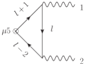
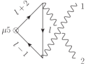
Figure 1: The two Feynman diagrams for the axial anomaly. The inserted axial current operator is labeled $\mu 5$ $\otimes$.

To obtain a comparison to chirality flow, we choose a set of polarizations, then use eqs. (A.0.5) and (A.0.6) to express the polarization vectors and momenta in terms of spinors, obtaining

$$\frac{ie^{2}}{(4\pi)^{2}}\mathop{\rm Tr}\Big{[}\gamma^{5}\not{1}\not{\epsilon}_{1,L}\not{2}\not{\epsilon}_{2_{R}}\Big{]} =\frac{ie^{2}}{(4\pi)^{2}}\frac{2}{{\color[rgb]{1,0,0}\langle}r_{1}1{\color[rgb]{1,0,0}\rangle}{\color[rgb]{0,0,1}[}2r_{2}{\color[rgb]{0,0,1}]}}\Big{[}-{\color[rgb]{1,0,0}\langle}1r_{1}{\color[rgb]{1,0,0}\rangle}{\color[rgb]{0,0,1}[}12{\color[rgb]{0,0,1}]}\underbrace{{\color[rgb]{1,0,0}\langle}22{\color[rgb]{1,0,0}\rangle}}_{0}{\color[rgb]{0,0,1}[}r_{2}1{\color[rgb]{0,0,1}]}+\underbrace{{\color[rgb]{0,0,1}[}11{\color[rgb]{0,0,1}]}}_{0}{\color[rgb]{1,0,0}\langle}r_{1}2{\color[rgb]{1,0,0}\rangle}{\color[rgb]{0,0,1}[}2r_{2}{\color[rgb]{0,0,1}]}{\color[rgb]{1,0,0}\langle}21{\color[rgb]{1,0,0}\rangle}\Big{]}$$

$$=0~{},$$

$$\frac{ie^{2}}{(4\pi)^{2}}\mathop{\rm Tr}\Big{[}\gamma^{5}\not{1}\not{\epsilon}_{1,L}\not{2}\not{\epsilon}_{2_{L}}\Big{]} =\frac{ie^{2}}{(4\pi)^{2}}\frac{2}{{\color[rgb]{1,0,0}\langle}r_{1}1{\color[rgb]{1,0,0}\rangle}{\color[rgb]{1,0,0}\langle}r_{2}2{\color[rgb]{1,0,0}\rangle}}\big{[}-{\color[rgb]{1,0,0}\langle}1r_{1}{\color[rgb]{1,0,0}\rangle}{\color[rgb]{0,0,1}[}12{\color[rgb]{0,0,1}]}{\color[rgb]{1,0,0}\langle}2r_{2}{\color[rgb]{1,0,0}\rangle}{\color[rgb]{0,0,1}[}21{\color[rgb]{0,0,1}]}+\underbrace{{\color[rgb]{0,0,1}[}11{\color[rgb]{0,0,1}]}}_{0}{\color[rgb]{1,0,0}\langle}r_{1}2{\color[rgb]{1,0,0}\rangle}\underbrace{{\color[rgb]{0,0,1}[}22{\color[rgb]{0,0,1}]}}_{0}{\color[rgb]{1,0,0}\langle}r_{2}1{\color[rgb]{1,0,0}\rangle}\big{]}$$

$$=\frac{-2ie^{2}}{(4\pi)^{2}}{\color[rgb]{0,0,1}[}12{\color[rgb]{0,0,1}]}{\color[rgb]{0,0,1}[}21{\color[rgb]{0,0,1}]}~{},$$ (4.0.2)

where we used the explicit representation of $\gamma^{5}$ in the chiral basis to separate the trace into two terms, and the cyclicity of the trace to write everything in terms of spinor inner products. Notice that the axial anomaly vanishes if the photons have opposite helicity.

We now go through the calculation leading up to eqs. (4.0.1) and (4.0.2) in chirality flow. It is easiest to set the polarizations and the reference vectors of the photons at the beginning. We choose $\epsilon_{1,\color[rgb]{0,0,1}{L}}$ with $r_{1}=2$ and $\epsilon_{2,\color[rgb]{1,0,0}{R}}$ with $r_{2}=1$. Using the QED vertex eq. (2.0.8), fermion propagator eq. (3.0.8), and splitting the trace of $\gamma$-matrices into two two-component traces, we have

$$i(p_{1}+p_{2})_{\mu}\includegraphics[scale={0.3},valign={c}]{Jaxodraw/QEDAxialAnomalyFeyn1LR}=\frac{2e^{2}}{{\color[rgb]{1,0,0}\langle}21{\color[rgb]{1,0,0}\rangle}{\color[rgb]{0,0,1}[}21{\color[rgb]{0,0,1}]}}\int\frac{d^{d}l_{[d]}}{(2\pi)^{d}}\left\{\includegraphics[scale={0.27},valign={c}]{Jaxodraw/QEDAxialAnomalyRchir4dDiag1LR}-\,\,\includegraphics[scale={0.27},valign={c}]{Jaxodraw/QEDAxialAnomalyLchir4dDiag1LR}\right.$$

$$+\mu^{2}\includegraphics[scale={0.27},valign={c}]{Jaxodraw/QEDAxialAnomalyRchirMu0Diag1LR}-\,\,\mu^{2}\includegraphics[scale={0.27},valign={c}]{Jaxodraw/QEDAxialAnomalyLchirMu0Diag1LR}+\mu^{2}\includegraphics[scale={0.27},valign={c}]{Jaxodraw/QEDAxialAnomalyRchirMu1Diag1LR}-\,\,\mu^{2}\includegraphics[scale={0.27},valign={c}]{Jaxodraw/QEDAxialAnomalyLchirMu1Diag1LR}$$

$$+\left.\mu^{2}\includegraphics[scale={0.27},valign={c}]{Jaxodraw/QEDAxialAnomalyRchirMu2Diag1LR}-\,\,\mu^{2}\includegraphics[scale={0.27},valign={c}]{Jaxodraw/QEDAxialAnomalyLchirMu2Diag1LR}\right\}\frac{1}{l_{[d]}^{2}(l+1)_{[d]}^{2}(l-2)_{[d]}^{2}}~{},$$ (4.0.3)

which is immediately simplified since all terms proportional to $\mu^{2}$ and parts of the first two chirality-flow diagrams vanish, due to ${\color[rgb]{1,0,0}\langle}ii{\color[rgb]{1,0,0}\rangle}={\color[rgb]{0,0,1}[}jj{\color[rgb]{0,0,1}]}=0$ and/or due to the Weyl equation, e.g. $\not{2}{\color[rgb]{1,0,0}|}2{\color[rgb]{1,0,0}\rangle}=0$ (here, and in the rest of the paper, we use the slash notation to refer to contraction with a Pauli matrix, see eq. (A.0.5)). Note how the clever choice of reference vectors helps remove many terms, as at tree level.

Next, we swap the arrow directions on all flow lines in the second chirality-flow diagram, and separate the momenta in the $l+1$ and $l-2$ momentum-dots of the first chirality-flow diagram to obtain

$$i(p_{1}+p_{2})_{\mu}\includegraphics[scale={0.3},valign={c}]{Jaxodraw/QEDAxialAnomalyFeyn1LR} =\frac{2e^{2}}{{\color[rgb]{1,0,0}\langle}21{\color[rgb]{1,0,0}\rangle}{\color[rgb]{0,0,1}[}21{\color[rgb]{0,0,1}]}}\int\frac{d^{d}l_{[d]}}{(2\pi)^{d}}\left\{\includegraphics[scale={0.27},valign={c}]{Jaxodraw/QEDAxialAnomalyRchir4dSimp1Diag1LR}+\includegraphics[scale={0.27},valign={c}]{Jaxodraw/QEDAxialAnomalyRchir4dSimp2Diag1LR}\right.$$

$$\left.+\includegraphics[scale={0.27},valign={c}]{Jaxodraw/QEDAxialAnomalyRchir4dSimpDiag1LR}-\,\,\includegraphics[scale={0.27},valign={c}]{Jaxodraw/QEDAxialAnomalyLchir4dSimpDiag1LR}\right\}\frac{1}{\left[l_{[d]}^{2}(l+1)_{[d]}^{2}(l-2)_{[d]}^{2}\right]}$$

$$=0$$ (4.0.4)

where, reading out the inner products, we see that the first two chirality-flow diagrams cancel each other, as do the two last two chirality-flow diagrams. Therefore, in chirality flow, the axial anomaly for opposite-helicity photons can be made to vanish before having to do the integration, with — similar to tree level — a large simplification coming from our choice of reference vectors.

Note that if the terms did not cancel, they would anyway individually vanish after integration. For example, the first chirality-flow diagram can be rewritten as

$$\int\frac{d^{d}l_{[d]}}{(2\pi)^{d}}\includegraphics[scale={0.27},valign={c}]{Jaxodraw/QEDAxialAnomalyRchir4dSimp1Diag1LR}\frac{1}{\left[l_{[d]}^{2}(l+1)_{[d]}^{2}(l-2)_{[d]}^{2}\right]} ={\color[rgb]{1,0,0}\langle}21{\color[rgb]{1,0,0}\rangle}{\color[rgb]{0,0,1}[}12{\color[rgb]{0,0,1}]}\int\frac{d^{d}l_{[d]}}{(2\pi)^{d}}\frac{{\color[rgb]{1,0,0}\langle}2{\color[rgb]{1,0,0}|}\bar{\not{l}}{\color[rgb]{0,0,1}|}1{\color[rgb]{0,0,1}]}{\color[rgb]{1,0,0}\langle}2{\color[rgb]{1,0,0}|}\bar{\not{l}}{\color[rgb]{0,0,1}|}1{\color[rgb]{0,0,1}]}}{\left[l_{[d]}^{2}(l+1)_{[d]}^{2}(l-2)_{[d]}^{2}\right]}~{},$$ (4.0.5)

which is a rank-two tensor integral. This integral can be solved using standard (d-dimensional) tensor analysis

$$\int\frac{d^{d}l_{[d]}}{(2\pi)^{d}}\frac{l_{[d]}^{\mu}l_{[d]}^{\nu}}{l_{[d]}^{2}(l+1)_{[d]}^{2}(l-2)_{[d]}^{2}} =C_{00}g^{\mu\nu}+C_{11}1^{\mu}1^{\nu}+C_{22}2^{\mu}2^{\nu}+C_{12}\left(1^{\mu}2^{\nu}+1^{\nu}2^{\mu}\right)~{},$$ (4.0.6)

where we used that $\bar{\not{l}}\equiv l_{[4]}^{\mu}\bar{\sigma}_{[4]\mu}=l_{[d]}^{\mu}\bar{\sigma}_{[4]\mu}$ due to the projective nature of the metric, eq. (3.0.3). However, every coefficient $C_{ij}$ multiplies a vanishing contribution, either due to the Weyl equation, e.g. $C_{11}{\color[rgb]{1,0,0}\langle}2{\color[rgb]{1,0,0}|}\bar{\not{1}}{\color[rgb]{0,0,1}|}1{\color[rgb]{0,0,1}]}{\color[rgb]{1,0,0}\langle}2{\color[rgb]{1,0,0}|}\bar{\not{1}}{\color[rgb]{0,0,1}|}1{\color[rgb]{0,0,1}]}=0$, or due to the Fierz identity, $C_{00}{\color[rgb]{1,0,0}\langle}2{\color[rgb]{1,0,0}|}\bar{\sigma}^{\mu}{\color[rgb]{0,0,1}|}1{\color[rgb]{0,0,1}]}{\color[rgb]{1,0,0}\langle}2{\color[rgb]{1,0,0}|}\bar{\sigma}_{\mu}{\color[rgb]{0,0,1}|}1{\color[rgb]{0,0,1}]}=2C_{00}{\color[rgb]{1,0,0}\langle}22{\color[rgb]{1,0,0}\rangle}{\color[rgb]{0,0,1}[}11{\color[rgb]{0,0,1}]}=0$. This exemplifies one of the major advantages of chirality flow for loop diagrams.

If we instead choose photon $2$ to be “left chiral” (have positive helicity), i.e., $\epsilon_{1,\color[rgb]{0,0,1}{L}}$ with $r_{1}=2$ and $\epsilon_{2,\color[rgb]{0,0,1}{L}}$ with $r_{2}=1$, we get

$$i(p_{1}+p_{2})_{\mu}\includegraphics[scale={0.3},valign={c}]{Jaxodraw/QEDAxialAnomalyFeyn1LL}=\frac{2e^{2}}{{\color[rgb]{1,0,0}\langle}21{\color[rgb]{1,0,0}\rangle}{\color[rgb]{1,0,0}\langle}12{\color[rgb]{1,0,0}\rangle}}\int\frac{d^{d}l_{[d]}}{(2\pi)^{d}}\left\{\includegraphics[scale={0.27},valign={c}]{Jaxodraw/QEDAxialAnomalyRchir4dDiag1LL}-\,\,\includegraphics[scale={0.27},valign={c}]{Jaxodraw/QEDAxialAnomalyLchir4dDiag1LL}\right.$$

$$+\mu^{2}\includegraphics[scale={0.27},valign={c}]{Jaxodraw/QEDAxialAnomalyRchirMu0Diag1LL}-\,\,\mu^{2}\includegraphics[scale={0.27},valign={c}]{Jaxodraw/QEDAxialAnomalyLchirMu0Diag1LL}+\mu^{2}\includegraphics[scale={0.27},valign={c}]{Jaxodraw/QEDAxialAnomalyRchirMu1Diag1LL}-\,\,\mu^{2}\includegraphics[scale={0.27},valign={c}]{Jaxodraw/QEDAxialAnomalyLchirMu1Diag1LL}$$

$$+\left.\mu^{2}\includegraphics[scale={0.27},valign={c}]{Jaxodraw/QEDAxialAnomalyRchirMu2Diag1LL}-\,\,\mu^{2}\includegraphics[scale={0.27},valign={c}]{Jaxodraw/QEDAxialAnomalyLchirMu2Diag1LL}\right\}\frac{1}{l_{[d]}^{2}(l+1)_{[d]}^{2}(l-2)_{[d]}^{2}}~{}.$$ (4.0.7)

Tensor integrals with three loop momenta, $I_{i_{1}i_{2}i_{3}}^{d}[l^{\mu}l^{\nu}l^{\rho}]$, can be reduced by using Platzer:2022nfu

$$=2l_{[4]}\cdot(1+2)_{[4]}\raisebox{-0.2pt}{\includegraphics[scale={0.3}]{Jaxodraw/1SigmaAnomalyRLl}}\,-\,l_{[4]}^{2}\raisebox{-0.2pt}{\includegraphics[scale={0.3}]{Jaxodraw/1SigmaAnomalyRLonetwo}}+i\underbrace{\epsilon^{\mu\nu\rho\eta}l_{\mu}(1_{\nu}+2_{\nu})l_{\rho}\bar{\sigma}_{\eta}}_{0}~{},$$ (4.0.8)

and we can then write the Lorentz structure as spinor products and strings to obtain (after cancellation of some terms)

$$i(p_{1}+p_{2})_{\mu}\includegraphics[scale={0.3},valign={c}]{Jaxodraw/QEDAxialAnomalyFeyn1LL} =\frac{2e^{2}{\color[rgb]{0,0,1}[}12{\color[rgb]{0,0,1}]}}{{\color[rgb]{1,0,0}\langle}12{\color[rgb]{1,0,0}\rangle}}\int\frac{d^{d}l_{[d]}}{(2\pi)^{d}}\Bigg{\{}\left(l_{[4]}^{2}-\mu^{2}\right)\left({\color[rgb]{1,0,0}\langle}2{\color[rgb]{1,0,0}|}\bar{\not{l}}{\color[rgb]{0,0,1}|}2{\color[rgb]{0,0,1}]}-{\color[rgb]{1,0,0}\langle}1{\color[rgb]{1,0,0}|}\bar{\not{l}}{\color[rgb]{0,0,1}|}1{\color[rgb]{0,0,1}]}\right)+2{\color[rgb]{1,0,0}\langle}1{\color[rgb]{1,0,0}|}\bar{\not{l}}{\color[rgb]{0,0,1}|}1{\color[rgb]{0,0,1}]}{\color[rgb]{1,0,0}\langle}2{\color[rgb]{1,0,0}|}\bar{\not{l}}{\color[rgb]{0,0,1}|}2{\color[rgb]{0,0,1}]}$$

$$\hphantom{=\frac{2e^{2}{\color[rgb]{0,0,1}[}12{\color[rgb]{0,0,1}]}}{{\color[rgb]{1,0,0}\langle}12{\color[rgb]{1,0,0}\rangle}}\int\frac{d^{d}l_{[d]}}{(2\pi)^{d}}}-2\mu^{2}{\color[rgb]{1,0,0}\langle}12{\color[rgb]{1,0,0}\rangle}{\color[rgb]{0,0,1}[}21{\color[rgb]{0,0,1}]}\Bigg{\}}\frac{1}{l_{[d]}^{2}(l+1)_{[d]}^{2}(l-2)_{[d]}^{2}}$$

$$=\frac{2e^{2}{\color[rgb]{0,0,1}[}12{\color[rgb]{0,0,1}]}}{{\color[rgb]{1,0,0}\langle}12{\color[rgb]{1,0,0}\rangle}}\left\{\int\frac{d^{d}l_{[d]}}{(2\pi)^{d}}\frac{{\color[rgb]{1,0,0}\langle}2{\color[rgb]{1,0,0}|}\bar{\not{l}}{\color[rgb]{0,0,1}|}2{\color[rgb]{0,0,1}]}-{\color[rgb]{1,0,0}\langle}1{\color[rgb]{1,0,0}|}\bar{\not{l}}{\color[rgb]{0,0,1}|}1{\color[rgb]{0,0,1}]}}{(l+1)_{[d]}^{2}(l-2)_{[d]}^{2}}\right.$$

$$\hphantom{=\frac{2e^{2}{\color[rgb]{0,0,1}[}12{\color[rgb]{0,0,1}]}}{{\color[rgb]{1,0,0}\langle}12{\color[rgb]{1,0,0}\rangle}}\Bigg{\{}}\left.+2\int\frac{d^{d}l_{[d]}}{(2\pi)^{d}}\frac{{\color[rgb]{1,0,0}\langle}1{\color[rgb]{1,0,0}|}\bar{\not{l}}{\color[rgb]{0,0,1}|}1{\color[rgb]{0,0,1}]}{\color[rgb]{1,0,0}\langle}2{\color[rgb]{1,0,0}|}\bar{\not{l}}{\color[rgb]{0,0,1}|}2{\color[rgb]{0,0,1}]}-\mu^{2}{\color[rgb]{1,0,0}\langle}12{\color[rgb]{1,0,0}\rangle}{\color[rgb]{0,0,1}[}21{\color[rgb]{0,0,1}]}}{l_{[d]}^{2}(l+1)_{[d]}^{2}(l-2)_{[d]}^{2}}\right\}~{},$$ (4.0.9)

where we used that $l_{[d]}^{2}=l_{[4]}^{2}-\mu^{2}$ from eq. (3.0.11). To solve this, we have to solve three integrals, which, using standard tensor reduction, we write as

$$\int\frac{d^{d}l_{[d]}}{(2\pi)^{d}}\frac{l_{[d]}^{\mu}}{(l+1)_{[d]}^{2}(l-2)_{[d]}^{2}} =C_{1}^{[0]}1^{\mu}+C_{2}^{[0]}2^{\mu}~{},$$

$$\int\frac{d^{d}l_{[d]}}{(2\pi)^{d}}\frac{l_{[d]}^{\mu}l_{[d]}^{\nu}}{l_{[d]}^{2}(l+1)_{[d]}^{2}(l-2)_{[d]}^{2}} =C_{00}g^{\mu\nu}+C_{11}1^{\mu}1^{\nu}+C_{22}2^{\mu}2^{\nu}+C_{12}\left(1^{\mu}2^{\nu}+1^{\nu}2^{\mu}\right)~{},$$

$$\int\frac{d^{d}l_{[d]}}{(2\pi)^{d}}\frac{\mu^{2}}{l_{[d]}^{2}(l+1)_{[d]}^{2}(l-2)_{[d]}^{2}} =C_{[\mu^{2}]}~{},$$ (4.0.10)

such that

$$i(p_{1}+p_{2})_{\mu}\includegraphics[scale={0.3},valign={c}]{Jaxodraw/QEDAxialAnomalyFeyn1LL} =2e^{2}{\color[rgb]{0,0,1}[}12{\color[rgb]{0,0,1}]}{\color[rgb]{0,0,1}[}21{\color[rgb]{0,0,1}]}\left(C_{1}^{[0]}-C_{2}^{[0]}+4C_{00}+2C_{12}{\color[rgb]{1,0,0}\langle}12{\color[rgb]{1,0,0}\rangle}{\color[rgb]{0,0,1}[}21{\color[rgb]{0,0,1}]}-2C_{[\mu^{2}]}\right)~{},$$ (4.0.11)

where it was again obvious due to the Weyl equation that not all tensor coefficients were required. Using eq. (3.0.12) for the integral with $\mu^{2}$, and calculating the tensor coefficients using Davydychev:1991va ; Giele:2004iy ; Platzer:2012oneloop ; Patel:2015tea ; Patel:2016fam ; Shtabovenko:2016whf we find

$$C_{1}^{[0]}-C_{2}^{[0]}+4C_{00}+2C_{12}{\color[rgb]{1,0,0}\langle}12{\color[rgb]{1,0,0}\rangle}{\color[rgb]{0,0,1}[}21{\color[rgb]{0,0,1}]} =0~{}, C_{[\mu^{2}]} =\frac{1}{2}\frac{i}{(4\pi)^{2}}~{},$$ (4.0.12)

and therefore we obtain the known result for the anomaly, eq. (4.0.2)

$$i(p_{1}+p_{2})_{\mu}\includegraphics[scale={0.3},valign={c}]{Jaxodraw/QEDAxialAnomalyFeyn1LL} =-\frac{2ie^{2}}{(4\pi)^{2}}{\color[rgb]{0,0,1}[}12{\color[rgb]{0,0,1}]}{\color[rgb]{0,0,1}[}21{\color[rgb]{0,0,1}]}~{}.$$ (4.0.13)

This example shows many of the features of chirality flow at one loop. We saw that many terms vanished due to the choice of reference vector, as well as a transparent simplification of the tensor reduction.

Though it was not required in this example, we may also need to take some care with chirality-flow arrows and minus signs at one loop (see the discussion of the fermion self-energy in section 4.2). This, along with other details of one-loop chirality-flow calculations, will be discussed below.

4.1 Reduction of tensor integrals

The method of performing one-loop calculations with chirality flow explored here is traditional in the sense that we do not exploit unitarity-based approaches, but rely on separating the numerator algebra from a tensor integral, which is then decomposed into the various tensor structures, and subsequently reduced to master integrals. The chirality-flow method allows to use spinor identities and equations of motion directly, such as to directly identify those tensor structures which will not contribute to an amplitude.

As we saw in the axial anomaly above, it is easy to identify which contributions of a tensor integral in chirality flow will vanish. A typical rank-$n$ tensor integral will occur as

$${\color[rgb]{1,0,0}\langle}i_{1}{\color[rgb]{1,0,0}|}\bar{\sigma}_{\mu_{1}}{\color[rgb]{0,0,1}|}j_{1}{\color[rgb]{0,0,1}]}\dots\color[rgb]{1,0,0}\langle i_{n}{\color[rgb]{1,0,0}|}\bar{\sigma}_{\mu_{n}}{\color[rgb]{0,0,1}|}j_{n}{\color[rgb]{0,0,1}]}I^{d}_{d_{1}\dots d_{k}}[l^{\mu_{1}}\dots l^{\mu_{n}}]~{},$$

$${\color[rgb]{1,0,0}\langle}i_{1}{\color[rgb]{1,0,0}|}\bar{\sigma}_{\mu_{1}}\sigma_{\mu_{2}}{\color[rgb]{1,0,0}|}j_{1}{\color[rgb]{1,0,0}\rangle}\dots\color[rgb]{1,0,0}\langle i_{n}{\color[rgb]{1,0,0}|}\bar{\sigma}_{\mu_{n}}{\color[rgb]{0,0,1}|}j_{n}{\color[rgb]{0,0,1}]}I^{d}_{d_{1}\dots d_{k}}[l^{\mu_{1}}\dots l^{\mu_{n}}]~{},$$

$${\color[rgb]{1,0,0}\langle}i_{1}{\color[rgb]{1,0,0}|}\bar{\sigma}_{\mu_{1}}\sigma_{\mu_{2}}{\color[rgb]{1,0,0}|}j_{1}{\color[rgb]{1,0,0}\rangle}\dots\color[rgb]{0,0,1}[i_{n}{\color[rgb]{0,0,1}|}\sigma_{\mu_{n-1}}\bar{\sigma}_{\mu_{n}}{\color[rgb]{0,0,1}|}j_{n}{\color[rgb]{0,0,1}]}I^{d}_{d_{1}\dots d_{k}}[l^{\mu_{1}}\dots l^{\mu_{n}}]~{},$$

$$\text{etc.}~{},$$ (4.1.1)

and coefficients will vanish for one of three reasons. Either, they will vanish due to the Weyl equation, e.g., $\bar{\not{j}}_{1}{\color[rgb]{0,0,1}|}j_{1}{\color[rgb]{0,0,1}]}=0$, due to massless momenta being contracted with consecutive Pauli matrices, e.g. $\not{j}_{1}\bar{\not{j}}_{1}=j_{1}^{2}=0$, or from the Fierz identity contracting two spinor strings with a common spinor, e.g.

$${\color[rgb]{1,0,0}\langle}i_{1}{\color[rgb]{1,0,0}|}\bar{\sigma}^{\mu}{\color[rgb]{0,0,1}|}j_{1}{\color[rgb]{0,0,1}]}{\color[rgb]{0,0,1}[}j_{1}{\color[rgb]{0,0,1}|}\sigma_{\mu}{\color[rgb]{1,0,0}|}i_{2}{\color[rgb]{1,0,0}\rangle}=2{\color[rgb]{1,0,0}\langle}i_{1}i_{2}{\color[rgb]{1,0,0}\rangle}{\color[rgb]{0,0,1}[}j_{1}j_{1}{\color[rgb]{0,0,1}]}=0~{},$$ (4.1.2)

where we define a string of spinors to be a sequence like ${\color[rgb]{1,0,0}\langle}i_{1}{\color[rgb]{1,0,0}|}\bar{\sigma}^{\mu}{\color[rgb]{0,0,1}|}j_{1}{\color[rgb]{0,0,1}]}$ which starts and ends with spinors, possibly with (many) Pauli matrices in between.

In general, the number of contributing structures in a tensor integral is dependent on the choice of gauge or spin reference momenta, and, like at tree level, choosing these wisely can significantly reduce the amount of work required to do the calculation.

Additionally, in chirality flow we are sometimes able to reduce the rank of a tensor integral by using equations such as eq. (4.0.8). In Platzer:2022nfu , we showed how to reduce strings of multiple momentum-dots into simpler building blocks, using e.g.

$$=l_{[4]}^{2}\raisebox{-0.2pt}{\includegraphics[scale={0.3}]{Jaxodraw/0SigmaRR}}~{},\quad\text{and}$$

$$=2l_{[4]}\cdot p_{[4]}\raisebox{-0.2pt}{\includegraphics[scale={0.3}]{Jaxodraw/1SigmaGenplRL}}\,-\,l_{[4]}^{2}\raisebox{-0.2pt}{\includegraphics[scale={0.3}]{Jaxodraw/1SigmaGenpRL}}~{},$$ (4.1.3)

where the former occurs in diagrams like

$$\includegraphics[scale={0.3},valign={c}]{Jaxodraw/ScalarFFloopvertex}~{},$$

while the latter appears in e.g. the axial anomaly calculation of the previous section. To use these relations, recall that the momenta on the denominator are d-dimensional, so we have to convert the four-dimensional dot products of eq. (4.1.3) to d-dimensional ones using

$$l_{[4]}^{2} =l_{[d]}^{2}+\mu^{2}~{}, 2l_{[4]}\cdot p_{[4]} =2l_{[d]}\cdot p_{[d]}=(l+p)^{2}_{[d]}-l_{[d]}^{2}-p^{2}_{[d]}$$ (4.1.4)

where we used that $p$ is strictly four-dimensional, so $p_{[4]}=p_{[d]}$. For a full set of relations which can reduce the rank of a tensor integral, see Platzer:2022nfu . Reduction methods of tensor integrals along the lines of Giele:2004iy ; Platzer:2012oneloop then allow us to directly reduce coefficients of individual tensor structures.

4.2 Abelian gauge theories

One-loop diagrams in abelian theories can be separated into two categories, diagrams like the axial anomaly in section 4 which have a purely fermionic loop, and diagrams which have a mixture of fermions and bosons in the loop.

For the former case, the procedure is simple, draw the chirality-flow diagram as at tree level Lifson:2020pai ; Alnefjord:2020xqr , putting arrows in their natural position, i.e., against the fermion flow. Then perform the integral, making use of the simplifications from section 4.1. The rest of this section deals with the second class of loops, those with bosons and fermions, and show that these can also be handled.

Loops with a single fermion line:

The simplest example of such a diagram is the self-energy of a massless fermion in the Feynman gauge. There are two diagrams for this process, one in which the fermion emits and reabsorbs the gauge boson (usually just called a photon below for convenience), and another in which it emits and reabsorbs the FDF scalar. However, the FDF-scalar contribution is proportional to $\Gamma^{M}\Gamma^{M}=0$, so we do not need to consider it.

If we consider just the Lorentz structure of the self-energy, and consider only a single chirality, we have e.g.

$$\sim\includegraphics[scale={0.3},valign={c}]{Jaxodraw/fermionSelfEnergyPhotonFlowLR}\sim\raisebox{-0.2pt}{\includegraphics[scale={0.3}]{Jaxodraw/fermionSelfEnergyFlowLR}}~{},$$ (4.2.1)

for the numerator structure. In the middle diagram, drawn to follow the Feynman diagram, we see that naively applying chirality flow to the diagram leads to either the photon having arrows in the same direction or the momentum-dot not having a continuous flow, both of which are avoided at tree level Lifson:2020pai . As we will see below, this simply introduces a minus sign into equations. In the right-hand diagram, we see that chirality flow quickly reduces the loop-level Lorentz structure to a simple tree-level chirality structure (i.e. a Lorentz structure which occurs in a tree-level chirality-flow diagram), without having to apply any anticommutation relations.

We now consider the general case of a single massless fermion emitting a virtual photon, possibly emitting more photons, and then reabsorbing the first virtual photon. The simplest version of this is the fermion self-energy, schematically given in eq. (4.2.1). Considering just the Lorentz algebra, we have for example

$$\rightarrow\,\,\bar{\tau}^{\nu}\Big{(}\not{p}+\not{l}\Big{)}\bar{\tau}_{\nu}=-\Big{(}\bar{\not{p}}+\bar{\not{l}}\Big{)}~{},$$ (4.2.2)

where the Pauli matrices with repeated index are removed using eq. (A.0.1), and the remaining Lorentz algebra is calculated using eqs. (A.0.2) and (A.0.3). Note that our normalization of the Pauli matrices in the fermion-photon vertex, eq. (2.0.8), gives the unusual prefactor of one on the right hand side (which would have read $2$ in the case of Dirac matrices or more traditionally-normalized Pauli matrices). In chirality flow, eq. (4.2.2) is drawn as

$$\rightarrow\,-\includegraphics[scale={0.3},valign={c}]{Jaxodraw/fermionSelfEnergyPhotonFlowLR}=-\raisebox{-0.2pt}{\includegraphics[scale={0.3}]{Jaxodraw/fermionSelfEnergyFlowLR}}~{}.$$ (4.2.3)

If the massless fermion emitted a photon before reabsorption, we instead obtain

$$\rightarrow\,\,\bar{\tau}^{\nu}\Big{(}\not{p}+\not{l}-\not{1}\Big{)}\bar{\tau}^{\nu_{1}}\Big{(}\not{p}+\not{l}\Big{)}\bar{\tau}_{\nu}+\mu^{2}\bar{\tau}^{\nu}\tau^{\nu_{1}}\bar{\tau}_{\nu}$$

$$=-\Big{(}\bar{\not{p}}+\bar{\not{l}}\Big{)}\tau^{\nu_{1}}\Big{(}\bar{\not{p}}+\bar{\not{l}}-\bar{\not{1}}\Big{)}-\mu^{2}\bar{\tau}^{\nu_{1}}~{},$$ (4.2.4)

using the same method as in eq. (4.2.2) for the Lorentz algebra. Note that we now have a $\mu^{2}$ term from the fermion propagator, and that in the first line we obtain $\mu^{2}$ instead of $-\mu^{2}$ due to the $\gamma^{5}$ matrices in the propagator. In chirality flow, this relation is

$$\rightarrow\,-\includegraphics[scale={0.3},valign={c}]{Jaxodraw/fermionSelfEnergyExtPhotonFlowdstructLR}-\mu^{2}\includegraphics[scale={0.3},valign={c}]{Jaxodraw/fermionSelfEnergyExtPhotonFlowdstructMu2LR}$$

$$=-\,\includegraphics[scale={0.3},valign={c}]{Jaxodraw/fermionSelfEnergyExtPhotonFlowLR}\,-\,\mu^{2}\includegraphics[scale={0.3},valign={c}]{Jaxodraw/fermionSelfEnergyExtPhotonFlowMu2LR}~{},$$ (4.2.5)

where we see that for chirality flow to look like a tree-level structure, we must reverse the order of the momentum-dots in the diagram.

In general, for a massless fermion emitting $n$ photons between emission and absorption of the virtual photon, the Lorentz structure will be sums of terms with the following form

$$\rightarrow\,\,(\mu^{2})^{n-k}\,\bar{\tau}^{\nu}\tau^{\nu_{1}}\dots\tau^{\nu_{2k+1}}\bar{\tau}_{\nu}=-(\mu^{2})^{n-k}\,\tau^{\nu_{2k+1}}\dots\tau^{\nu_{1}}~{},$$ (4.2.6)

where $k$ is an integer satisfying $\text{max}\left(0,\frac{n-1}{2}\right)\leq k\leq n$, we suppress the propagator momenta, and the sequence of Pauli matrices always goes $\tau$, $\tau\bar{\tau}\tau$, $\tau\bar{\tau}\tau\bar{\tau}\tau$ etc. Note that this relation only holds for an odd number of Pauli matrices, and that, like in eq. (4.2.5), the order of the Pauli matrices on the right-hand side of eq. (4.2.6) is reversed. If the fermion in eq. (4.2.6) is massive, then some powers of $\mu^{2}$ may be replaced by $m^{2}$, and the overall sign in this equation is no longer fixed and is calculated using eq. (3.0.8).

The other thing which could happen if the fermion is massive, is that the external fermions could have the same chirality, say left-left. (This may also happen if we for example replace one of the photons $1\dots n$ in diagrams like eq. (4.2.6) with a scalar particle.) In this case, there will be an even number of Pauli matrices between emission and absorption, it is easy to remove the repeated vector index using eq. (A.0.1), and the Feynman diagram will have Lorentz structures of the form

$$\sim\,\,m^{2r+1}(\mu^{2})^{q}\,\tau^{\nu}\bar{\tau}^{\nu_{1}}\dots\tau^{\nu_{2k}}\bar{\tau}_{\nu}=m^{2r+1}(\mu^{2})^{q}\,\delta^{{\dot{\alpha}}}_{~{}{\dot{\beta}}}\mathop{\rm Tr}\left(\bar{\tau}^{\nu_{1}}\dots\tau^{\nu_{2k}}\right)~{},$$ (4.2.7)

where $k,r$, and $q$ are non-negative integers satisfying $n/2\leq k\leq n$, $r=n-k-q\leq n/2$, and $q\leq n/2$, and the overall sign is determined using eq. (3.0.8).

As a simple example of eq. (4.2.7) we consider the diagram from eq. (4.2.5), but for the case of left-left chiralities coming from the replacement of a $\not{p}$ with a mass

$$\rightarrow\,m\delta^{{\dot{\alpha}}}_{~{}{\dot{\beta}}}\mathop{\rm Tr}\Big{[}\bar{\tau}^{\nu_{1}}\Big{(}\not{p}+\not{l}\Big{)}\Big{]}+m\delta^{{\dot{\alpha}}}_{~{}{\dot{\beta}}}\mathop{\rm Tr}\Big{[}\Big{(}\bar{\not{p}}+\bar{\not{l}}-\bar{\not{1}}\Big{)}\tau^{\nu_{1}}\Big{]}~{},$$ (4.2.8)

or in chirality flow

$$\rightarrow\,m\includegraphics[scale={0.3},valign={c}]{Jaxodraw/fermionSelfEnergyExtPhotondstruct1LL}+m\includegraphics[scale={0.3},valign={c}]{Jaxodraw/fermionSelfEnergyExtPhotondstruct2LL}~{},$$ (4.2.9)

where the chirality-flow arrows go against the fermion-flow arrows in order to get the correct sign, as in massive chirality flow Alnefjord:2020xqr .

While we have given only half of the chiralities explicitly, swapping the chiralities of the fermions in the above examples is trivial, since it is equivalent to swapping all solid lines for dotted ones and vice versa.

Loops with two or more fermion lines:

We now consider loops with two or more fermion lines. To set the chirality-flow lines consistently in these examples is analogous to the procedure in Alnefjord:2020xqr , and is perhaps easiest seen by example (we will give a systematic treatment afterwards). Consider the following box diagram, redrawn as a chirality-flow diagram,

$$\rightarrow\,\includegraphics[scale={0.35},valign={c}]{Jaxodraw/bubbleFlowPreFierzLLRR}~{},$$ (4.2.10)

where the chirality-flow lines have chirality-flow arrows opposing fermion-flow arrows, and photons are drawn as double lines which are not yet connected. We note that we cannot connect the photons’ flow lines yet, since their arrow directions do not match. To fix this, we use that the chirality-flow lines will always (at least eventually) end with spinors. Labeling the momenta of these end spinors $i$ and $j$, we can use

$${\color[rgb]{1,0,0}\langle}i{\color[rgb]{1,0,0}|}\bar{\tau}^{\mu}\Big{(}\not{q}-\not{l}\Big{)}\bar{\tau}^{\nu}{\color[rgb]{0,0,1}|}j{\color[rgb]{0,0,1}]}={\color[rgb]{0,0,1}[}j{\color[rgb]{0,0,1}|}\tau^{\nu}\Big{(}\bar{\not{q}}-\bar{\not{l}}\Big{)}\tau^{\mu}{\color[rgb]{1,0,0}|}i{\color[rgb]{1,0,0}\rangle}~{},$$ (4.2.11)

an example of eq. (A.0.4), to swap the chirality-flow arrows on the bottom line, obtaining

$$\rightarrow\,\includegraphics[scale={0.35},valign={c}]{Jaxodraw/bubbleFlowPostFierzNotJoinedLLRR}=\includegraphics[scale={0.35},valign={c}]{Jaxodraw/bubbleFlowPostFierzJoinedLLRR}~{},$$ (4.2.12)

where we first swapped the arrows, and then connected the photons using the Fierz identity, leading to a completed chirality-flow diagram. Note that we have, for the first time in this paper, a closed chirality-flow string. Such chirality-flow strings are simply traces of Pauli matrices, or equivalently, strings of inner products.

If the top fermion line of the box diagram is massive, for a given helicity configuration we will also have to calculate chirality-flow diagrams like

$$\rightarrow\,\raisebox{-0.53pt}{\includegraphics[scale={0.35}]{Jaxodraw/bubbleFlowPreFierzLLLR}}~{}.$$ (4.2.13)

In this case, we can already use the Fierz identity to join the rightmost photon, obtaining

$$\rightarrow\,\raisebox{-0.53pt}{\includegraphics[scale={0.35}]{Jaxodraw/bubbleFlowHalfFierzLLLR}}~{},$$ (4.2.14)

which has two strings of chirality-flow lines, one from the bottom right to the top left (string 1), and the other from the top right to the bottom left (string 2). To connect these two together, we need to use eq. (A.0.4) to flip the arrows on one string or the other. If we flip it on the string of lines containing the momentum-dot, there is an odd number of inner products, so a minus sign will be introduced. Alternatively, we can flip the arrows on string 1 which has two inner products, and therefore will not introduce a minus sign, obtaining

$$\rightarrow\,\raisebox{-0.53pt}{\includegraphics[scale={0.35}]{Jaxodraw/bubbleFlowHalfFierzSwapLLLR}}=\raisebox{-0.53pt}{\includegraphics[scale={0.35}]{Jaxodraw/bubbleFlowPostFierzLLLR}}~{}.$$ (4.2.15)

Note that the final result is independent of where we swap the arrows.

In a general one-loop abelian Feynman diagram with multiple fermion lines in the loop, the general procedure to set the arrow directions is:

1. Draw the chirality-flow lines for each fermion line with chirality flow opposing fermion flow. (Do not use the Fierz identity to attach fermion lines together yet.)

2. Choose a photon to be Fierzed first. If needed, use eq. (A.0.4) to swap the arrow directions of one of the fermion lines containing this photon, and then use the Fierz identity to connect the flow lines. Note that the chirality-flow lines will always, eventually, end in spinors, even if these spinor ends are not explicitly included in the loop calculation, so eq. (A.0.4) will always hold.

3. To Fierz further photons, either repeat step 2 with the fermion lines replaced by the strings of chirality-flow lines, or use one of eqs. (4.2.6) or (4.2.7), whichever is appropriate.

4. Repeat step 3 until all photons are replaced with joined chirality-flow lines. This will give a completed one-loop chirality-flow diagram with fully simplified Lorentz structure.

General $R_{\xi}$ gauge:

Since the gauge-parameter (in)dependence is an important cross-check of any perturbative calculation, we here comment on the general $R_{\xi}$ gauge, for which the photon propagator is

$$\raisebox{-0.2pt}{\includegraphics[scale={0.3}]{Jaxodraw/PhotonProp}}=-\frac{i}{p^{2}_{[4]}}\left(g^{\mu\nu}_{[4]}-(1-\xi)\frac{p^{\mu}_{[4]}p^{\nu}_{[4]}}{p^{2}_{[4]}}\right)~{},$$ (4.2.16)

in four dimensions. This is straightforwardly translated into chirality flow by recalling that $p^{\mu}$ will always be contracted with a Pauli matrix, thus becoming a momentum-dot (see eq. (2.0.11))

$$\rightarrow\,\,-\frac{i}{p^{2}_{[4]}}\left(\raisebox{-0.2pt}{\includegraphics[scale={0.3}]{Jaxodraw/PhotonPropFlowa}}\ -\ (1-\xi)\frac{1}{2p^{2}_{[4]}}\raisebox{-0.2pt}{\includegraphics[scale={0.3}]{Jaxodraw/PhotonPropFlowpa}}\right)~{},\quad\text{or}$$

$$\rightarrow\,\,-\frac{i}{p^{2}_{[4]}}\left(\raisebox{-0.2pt}{\includegraphics[scale={0.3}]{Jaxodraw/PhotonPropFlowb}}\ -\ (1-\xi)\frac{1}{2p^{2}_{[4]}}\raisebox{-0.2pt}{\includegraphics[scale={0.3}]{Jaxodraw/PhotonPropFlowpb}}\right)~{}.$$ (4.2.17)

If the internal photon is part of a loop, eq. (4.2.16) is modified using the $-2\epsilon$-SRs, eqs. (3.0.6) and (3.0.7), to also add the propagator of the FDF scalar

$$=-\frac{i}{p^{2}_{[d]}}\left(g^{\mu\nu}_{[d_{s}]}-(1-\xi)\frac{p^{\mu}_{[d]}p^{\nu}_{[d]}}{p^{2}_{[d]}}\right)$$

$$=\underbrace{-\frac{i}{p^{2}_{[d]}}\left(g^{\mu\nu}_{[4]}-(1-\xi)\frac{p^{\mu}_{[4]}p^{\nu}_{[4]}}{p^{2}_{[d]}}\right)}_{\text{4d photon}}\quad\,\underbrace{-\frac{i}{p^{2}_{[d]}}\left(G^{MN}+\mu^{2}(1-\xi)\frac{Q^{M}Q^{N}}{p^{2}_{[d]}}\right)}_{\text{FDF scalar}}~{}.$$ (4.2.18)

Treating the FDF-scalar as a separate particle to the photon, we obtain eq. (4.2.17) as the flow representation of the photon, and a trivial prefactor as the flow representation of the FDF-scalar.

FDF scalars:

One key feature of FDF is the appearance of FDF scalars, which have their own Feynman rules (see Fazio:2014xea ). In abelian theories, there are two new rules, the propagator for the FDF scalar just discussed, and the interaction vertex of the FDF-scalar with a fermion

$$=ie\gamma^{5}\Gamma^{M}=\,ie\Gamma^{M}\begin{pmatrix}-\includegraphics[scale={0.3},valign={c}]{Jaxodraw/FermionFDFScalarFlowL}&0\\ 0&\includegraphics[scale={0.3},valign={c}]{Jaxodraw/FermionFDFScalarFlowR}\end{pmatrix}~{},$$ (4.2.19)

where the flow rule is the same as any scalar (up to the coupling) and the sign on the left-chiral part coming from $\gamma^{5}$.

Looking ahead to non-abelian theories, we find that the Feynman rules for FDF-scalars only add ingredients we already know how to treat, such as four-dimensional metrics (eq. (2.0.9)) and four-dimensional momenta (eq. (2.0.11)), together with some of the $-2\epsilon$-SRs which will contract to either $0$ or $\pm 1$. Therefore, FDF scalars are a non-complication from the perspective of chirality flow. We also note that counterterms do not introduce any new structure which the chirality-flow formalism would not be able to handle.

4.3 Non-abelian gauge theories

To go from loops in an abelian theory to those in a non-abelian theory is straightforward in chirality flow. As we will see below, there is essentially nothing new to the non-abelian case compared to the abelian case, only more terms to keep track of.

4.3.1 QCD

The aim of this section is to explore what chirality-flow structures we obtain in QCD, and argue that we can always consistently set chirality-flow arrows. We will see that all non-abelian Feynman diagrams have a Lorentz structure which is either composed of the tree-level structures already described in Lifson:2020pai ; Alnefjord:2020xqr , or of the same structures as in an abelian gauge theory like QED, discussed in the previous section.

Compared to abelian gauge theories like QED, there are two new features in QCD: the addition of ghosts, and the non-abelian vertices. The ghosts have a scalar propagator and couple to a gluon with a momentum which is easily flowed (see eq. (2.0.11)), so they are not a complication.

The non-abelian vertices are built from Lorentz structures we have already treated. This can be seen using a simple illustrative example like

$$\includegraphics[scale={0.3},valign={c}]{Jaxodraw/FermionExtGluonLoopLR}~{}.$$ (4.3.1)

To understand the flow structure of this diagram, we first recall the Lorentz structure of the triple gluon vertex

$$=\;i\frac{g_{s}}{\sqrt{2}}if^{a_{1}a_{2}a_{3}}\Big{(}g^{\mu_{1}\mu_{2}}(p_{1}-p_{2})^{\mu_{3}}+g^{\mu_{2}\mu_{3}}(p_{2}-p_{3})^{\mu_{1}}+g^{\mu_{3}\mu_{1}}(p_{3}-p_{1})^{\mu_{2}}\Big{)},$$

$$\rightarrow\;i\frac{g_{s}}{\sqrt{2}}if^{a_{1}a_{2}a_{3}}\left(\includegraphics[scale={0.325},valign={c}]{Jaxodraw/MS/3GluonVertex_HelFlow1}\!\!\!+\includegraphics[scale={0.325},valign={c}]{Jaxodraw/MS/3GluonVertex_HelFlow2}\!\!\!+\includegraphics[scale={0.325},valign={c}]{Jaxodraw/MS/3GluonVertex_HelFlow3}\!\!\!\right)~{}.$$ (4.3.2)

Applying this vertex to the loop diagram in eq. (4.3.1), we find (using Feynman gauge and a massless fermion for simplicity)

$$\rightarrow\,\,\includegraphics[scale={0.3},valign={c}]{Jaxodraw/FermionExtGluonLoopFlow1LR}-\includegraphics[scale={0.3},valign={c}]{Jaxodraw/FermionExtGluonLoopFlow2LR}+\includegraphics[scale={0.3},valign={c}]{Jaxodraw/FermionExtGluonLoopFlow3LR}~{},$$ (4.3.3)

for the Lorentz structure. Here we see that the first and third terms already have tree-level Lorentz structure, while the middle term has the “abelian” Lorentz structure from eq. (4.2.3) (hence the minus sign), multiplied by a disconnected structure. Therefore, all of the Lorentz structures in this QCD diagram are either tree-level structures from Lifson:2020pai , or built from the Lorentz structures already encountered in abelian gauge theories, and setting a consistent arrow direction is straightforward.

This conclusion holds for any general QCD one-loop diagram. This is because the three- and four-gluon vertices, eqs. (4.3.2) and (A.0.8), break up the Lorentz structure into simpler pieces which either: break the loop Lorentz structure into a tree-level Lorentz structure, or create loop Lorentz structures of the form of eqs. (4.2.6) and (4.2.7). Further, the ghosts and FDF scalars only add 4d metrics and momenta multiplied by $-2\epsilon$-SRs objects, so again break up the Lorentz structure into either trees or structures like eqs. (4.2.6) and (4.2.7).

Finally, since the external gluons can have either set of arrow directions without introducing a minus sign, setting arrows is either the same as at tree level, or follows the abelian case in section 4.2.

4.3.2 Other non-abelian theories

Other non-abelian theories will similarly be easily flowable as long as they contain Feynman rules with 4d objects like scalars, Weyl and Dirac spinors, polarization vectors, momenta, the metric, $\gamma^{\mu}$, and $\gamma^{5}$, together with the $-2\epsilon$-SRs. In the Standard Model, the other non-abelian theory is the electroweak theory, which behaves like QCD but has the addition of massive polarization vectors, chiral vertices, and more (loop-level) scalars.

Chiral vertices and massive polarization vectors were both discussed in Alnefjord:2020xqr . The chiral vertices are easiest understood by drawing the chirality-flow arrow opposing the fermion-flow arrow, giving

$$\gamma^{\mu}P_{\color[rgb]{0,0,1}{L}} \rightarrow\,\,\sqrt{2}\includegraphics[scale={0.3},valign={c}]{Jaxodraw/FermionVectorVertexL}~{}, \gamma^{\mu}P_{\color[rgb]{1,0,0}{R}} \rightarrow\,\,\sqrt{2}\includegraphics[scale={0.3},valign={c}]{Jaxodraw/FermionVectorVertexR}~{},$$ (4.3.4)

for $P_{\color[rgb]{1,0,0}{R}/\color[rgb]{0,0,1}{L}}=(1\mathbin{\ensurestackMath{\abovebaseline[-3.4pt]{\stackunder[-3.5pt]{\color[rgb]{1,0,0}+}{\color[rgb]{0,0,1}-}}}}\gamma^{5})/2$. After having made this assignment, all arrow swaps can be done as previously described.

The massive polarization vectors are given in eq. (A.0.7), with the transverse polarization vectors having the same structure as massless polarization vectors, while the longitudinal polarization vector corresponds to a momentum-dot. Therefore, one consequence of longitudinal polarization vectors is that we can obtain closed chirality-flow strings. For example, the axial anomaly with longitudinally-polarized $W$ bosons has the following Lorentz structure

$$i(1_{\mu}+2_{\mu})\includegraphics[scale={0.26},valign={c}]{Jaxodraw/EWAxialAnomalyFeyn100} \rightarrow\,\,\includegraphics[scale={0.26},valign={c}]{Jaxodraw/EWAxialAnomaly4dDiag100}+\mu^{2}\includegraphics[scale={0.26},valign={c}]{Jaxodraw/EWAxialAnomalyMu2Diag100}~{},$$ (4.3.5)

where both terms have closed chirality-flow strings. (The chiral projectors ensure that these are the only two Lorentz structures in the calculation.) These closed flow loops can either be written as sums of spinor products or as traces of Pauli matrices.

Finally, we comment on the fermion self-energy in a theory with a spontaneously broken symmetry like the Standard Model. In the Feynman gauge, as shown in eq. (4.2.3), the contribution from a boson of mass $m$ to the self-energy is

$$\sim\,g^{2}\int\frac{d^{d}l_{[d]}}{(2\pi)^{d}}\frac{\raisebox{-0.2pt}{\includegraphics[scale={0.3}]{Jaxodraw/fermionSelfEnergyFlowLR}}}{(l^{2}-m^{2})(l+p)^{2}}~{},$$ (4.3.6)

where we label the generic coupling factors as $g^{2}$ and ignore factors of $-1$, $i$ and $\sqrt{2}$. Note that it is obvious in chirality flow that this has exactly the same structure as the contribution from a Goldstone boson of mass $m_{G}=m$

$$\sim\,(g^{\prime})^{2}\int\frac{d^{d}l_{[d]}}{(2\pi)^{d}}\frac{\raisebox{-0.2pt}{\includegraphics[scale={0.3}]{Jaxodraw/fermionSelfEnergyFlowLR}}}{(l^{2}-m^{2})(l+p)^{2}}~{},$$ (4.3.7)

where $g^{\prime}\neq g$ is the coupling of the Goldstone to the fermion. This type of transparency is one of the nice features of chirality flow at both tree and one-loop level.

Further, in a general $R_{\xi}$ gauge, we can use relations such as eq. (4.1.3) to relate the extra terms to the Goldstone contribution. We envisage that the cancellation of gauge-parameter dependence can thus be made more manifest by using chirality flow.

5 Conclusion

In this paper we have studied the chirality-flow formalism at one-loop order. We conclude that many of the simplifications seen at tree-level can be retained, at least in the four-dimensional formulation of the 4$d$ helicity scheme. In particular, the Lorentz algebra can be elegantly simplified, and Feynman diagrams can be made to vanish by picking adequate reference vectors for external gauge bosons and massive spinors.

Beyond this, we find that the tensor reduction procedure is also simplified for one of two reasons. Either, because we reduce the number of required coefficients in the tensor decomposition, or because we reduce the rank of the tensor integral. The former may happen either directly due to the Weyl equation or when applying the Fierz identity, while the latter occurs when multiple momentum-dots containing the loop momentum are contracted together.

Appendix A Additional chirality-flow rules

In this section we collect the chirality-flow rules required for this paper which are not stated in the main text. Additional chirality-flow rules can be found in Lifson:2020pai ; Alnefjord:2020xqr .

We begin with some algebra relations required to prove eqs. (4.2.2 - 4.2.9). The vector indices of the Pauli matrices can be contracted using

$$\tau_{\mu}^{\dot{\alpha}\beta}\bar{\tau}^{\mu}_{\gamma\dot{\eta}} =\delta_{\gamma}^{\ \beta}\delta_{\ \dot{\eta}}^{\dot{\alpha}}\,, \bar{\tau}^{\mu}_{\alpha\dot{\beta}}\bar{\tau}_{\mu,\gamma\dot{\eta}} =\epsilon_{\alpha\gamma}\epsilon_{\dot{\beta}\dot{\eta}}\,, \tau^{\mu,\dot{\alpha}\beta}\tau_{\mu}^{\dot{\gamma}\eta} =\epsilon^{\dot{\alpha}\dot{\gamma}}\epsilon^{\beta\eta}\,,$$ (A.0.1)

while a $\tau$ can be turned into a $\bar{\tau}$ or vice versa using

$$\bar{\tau}^{\mu}_{\alpha\dot{\beta}} =\epsilon_{\alpha\gamma}\epsilon_{\dot{\beta}\dot{\eta}}\tau^{\mu,\dot{\eta}\gamma}~{}, \tau^{\mu,\dot{\alpha}\beta} =\epsilon^{\dot{\alpha}\dot{\gamma}}\epsilon^{\beta\eta}\bar{\tau}^{\mu}_{\eta\dot{\gamma}}~{},$$ (A.0.2)

where the index positions are crucial, because

$$\epsilon_{\alpha\beta}\epsilon^{\beta\gamma} =\delta_{\alpha}^{\ \gamma}~{}, \epsilon^{\dot{\alpha}\dot{\beta}}\epsilon_{\dot{\beta}\dot{\gamma}} =\delta^{\dot{\alpha}}_{\ \dot{\gamma}}~{}, \epsilon_{\alpha\beta} =-\epsilon_{\beta\alpha}~{}, \epsilon_{\dot{\beta}\dot{\gamma}} =-\epsilon_{\dot{\gamma}\dot{\beta}}~{}.$$ (A.0.3)

Next, we recall the equations behind arrow flips. A string of chirality-flow lines can have all of its arrows flipped using one of

$${\color[rgb]{1,0,0}\langle}i{\color[rgb]{1,0,0}|}\bar{\tau}^{\mu_{1}}\dots\bar{\tau}^{\mu_{2n+1}}{\color[rgb]{0,0,1}|}j{\color[rgb]{0,0,1}]} ={\color[rgb]{0,0,1}[}j{\color[rgb]{0,0,1}|}\tau^{\mu_{2n+1}}\dots\tau^{\mu_{1}}{\color[rgb]{1,0,0}|}i{\color[rgb]{1,0,0}\rangle}~{},$$

$${\color[rgb]{1,0,0}\langle}i{\color[rgb]{1,0,0}|}\bar{\tau}^{\mu_{1}}\dots\tau^{\mu_{2n}}{\color[rgb]{1,0,0}|}j{\color[rgb]{1,0,0}\rangle} =-{\color[rgb]{1,0,0}\langle}j{\color[rgb]{1,0,0}|}\bar{\tau}^{\mu_{2n}}\dots\tau^{\mu_{1}}{\color[rgb]{1,0,0}|}i{\color[rgb]{1,0,0}\rangle}~{},$$

$${\color[rgb]{0,0,1}[}i{\color[rgb]{0,0,1}|}\tau^{\mu_{1}}\dots\bar{\tau}^{\mu_{2n}}{\color[rgb]{0,0,1}|}j{\color[rgb]{0,0,1}]} =-{\color[rgb]{0,0,1}[}j{\color[rgb]{0,0,1}|}\tau^{\mu_{2n}}\dots\bar{\tau}^{\mu_{1}}{\color[rgb]{0,0,1}|}i{\color[rgb]{0,0,1}]}~{},$$ (A.0.4)

where we note that the Pauli matrices stand in a sequence $\tau\bar{\tau}\tau\dots$ or $\bar{\tau}\tau\bar{\tau}\dots$. In practice, when swapping the chirality-flow arrows on a string of flow lines, if the endpoints of the string have the same chirality (line type) then a minus sign is required, while if the endpoints are of opposite chirality (line type) then no minus sign is needed.

In the spinor helicity formalism, for example when converting the axial anomaly from eq. (4.0.1) to eq. (4.0.2), it can be useful to write all objects as (sums of) outer products of spinors. For example, every momentum can be written as

$$\not{p}\equiv p^{\mu}\sigma_{\mu} \overset{p_{i}^{2}=0}{=}\sum_{i}{\color[rgb]{0,0,1}|}i{\color[rgb]{0,0,1}]}{\color[rgb]{1,0,0}\langle}i{\color[rgb]{1,0,0}|}~{}, \bar{\not{p}}\equiv p^{\mu}\bar{\sigma}_{\mu} \overset{p_{i}^{2}=0}{=}\sum_{i}{\color[rgb]{1,0,0}|}i{\color[rgb]{1,0,0}\rangle}{\color[rgb]{0,0,1}[}i{\color[rgb]{0,0,1}|}~{},$$ (A.0.5)

where we used that $p=\sum_{i}p_{i}$ with $p_{i}^{2}=0$ to write a massive momentum $p$ as a sum of massless ones (see eq. (2.0.4)), and the massless polarization vectors in eq. (2.0.3) can be written as

$$\not{\epsilon}_{\color[rgb]{0,0,1}{L}}(p_{i},r) =\frac{{\color[rgb]{0,0,1}|}i{\color[rgb]{0,0,1}]}{\color[rgb]{1,0,0}\langle}r{\color[rgb]{1,0,0}|}}{{\color[rgb]{1,0,0}\langle}ri{\color[rgb]{1,0,0}\rangle}} \bar{\not{\epsilon}}_{\color[rgb]{0,0,1}{L}}(p_{i},r) =\frac{{\color[rgb]{1,0,0}|}r{\color[rgb]{1,0,0}\rangle}{\color[rgb]{0,0,1}[}i{\color[rgb]{0,0,1}|}}{{\color[rgb]{1,0,0}\langle}ri{\color[rgb]{1,0,0}\rangle}}~{},$$ or

$$\not{\epsilon}_{\color[rgb]{1,0,0}{R}}(p_{i},r) =\frac{{\color[rgb]{0,0,1}|}r{\color[rgb]{0,0,1}]}{\color[rgb]{1,0,0}\langle}i{\color[rgb]{1,0,0}|}}{{\color[rgb]{0,0,1}[}ir{\color[rgb]{0,0,1}]}} \bar{\not{\epsilon}}_{\color[rgb]{1,0,0}{R}}(p_{i},r) =\frac{{\color[rgb]{1,0,0}|}i{\color[rgb]{1,0,0}\rangle}{\color[rgb]{0,0,1}[}r{\color[rgb]{0,0,1}|}}{{\color[rgb]{0,0,1}[}ir{\color[rgb]{0,0,1}]}}~{}.$$ or (A.0.6)

In our discussion of non-abelian theories, we require the polarization vectors of outgoing massive particles

$$\left(\epsilon^{\mu}_{+}(p^{\flat},q)\right)^{*} \longrightarrow \frac{1}{{\color[rgb]{1,0,0}\langle}qp^{\flat}{\color[rgb]{1,0,0}\rangle}}\!\raisebox{-0.25pt}{\includegraphics[scale={0.355}]{Jaxodraw/MS/ZExtFlowPlaRevCol}} \frac{1}{{\color[rgb]{1,0,0}\langle}qp^{\flat}{\color[rgb]{1,0,0}\rangle}}\!\raisebox{-0.25pt}{\includegraphics[scale={0.355}]{Jaxodraw/MS/ZExtFlowPlaCol}}\!\!\!\!,$$ or

$$\left(\epsilon^{\mu}_{-}(p^{\flat},q)\right)^{*} \longrightarrow \frac{1}{{\color[rgb]{0,0,1}[}p^{\flat}q{\color[rgb]{0,0,1}]}}\raisebox{-0.25pt}{\includegraphics[scale={0.355}]{Jaxodraw/MS/ZExtFlowMiaRevCol}} \frac{1}{{\color[rgb]{0,0,1}[}p^{\flat}q{\color[rgb]{0,0,1}]}}\raisebox{-0.25pt}{\includegraphics[scale={0.355}]{Jaxodraw/MS/ZExtFlowMiaCol}}\!\!\!\!,$$ or

$$\left(\epsilon^{\mu}_{0}(p^{\flat},q)\right)^{*} \longrightarrow \frac{1}{m\sqrt{2}}\!\raisebox{-0.25pt}{\includegraphics[scale={0.355}]{Jaxodraw/MS/ZExtFlow0dotCol}} \frac{1}{m\sqrt{2}}\!\raisebox{-0.25pt}{\includegraphics[scale={0.355}]{Jaxodraw/MS/ZExtFlow0dotRevCol}}\!\!\!\!,$$ or (A.0.7)

as well as the four-gluon vertex

$$=\;\;i\left(\!\frac{g_{s}}{\sqrt{2}}\right)^{\!\!2}\!\!\;\sum\limits_{Z(2,3,4)}if^{a_{1}a_{2}b}if^{ba_{3}a_{4}}\;\Big{(}g^{\mu_{1}\mu_{3}}g^{\mu_{2}\mu_{4}}-g^{\mu_{1}\mu_{4}}g^{\mu_{2}\mu_{3}}\Big{)}\;,$$

$$\rightarrow\;\;i\left(\!\frac{g_{s}}{\sqrt{2}}\right)^{\!\!2}\!\!\;\sum\limits_{Z(2,3,4)}if^{a_{1}a_{2}b}if^{ba_{3}a_{4}}\left(\includegraphics[scale={0.225},valign={c}]{Jaxodraw/MS/4GluonVertex_Kin13}-\includegraphics[scale={0.225},valign={c}]{Jaxodraw/MS/4GluonVertex_Kin14}\right)~{},$$ (A.0.8)

where $Z(2,3,4)$ denotes the set of cyclic permutations of the integers $2,3,4$, and in both cases the arrow directions which give a continuous flow in a given diagram are chosen.

References

• (1) A. Lifson, C. Reuschle and M. Sjodahl, The chirality-flow formalism, Eur. Phys. J. C 80 (2020) 1006 [2003.05877].
• (2) J. Alnefjord, A. Lifson, C. Reuschle and M. Sjodahl, The chirality-flow formalism for the standard model, 2011.10075.
• (3) A. Lifson, M. Sjodahl and Z. Wettersten, Automating scattering amplitudes with chirality flow, Eur. Phys. J. C 82 (2022) 535 [2203.13618].
• (4) S. Plätzer and M. Sjodahl, Amplitude Factorization in the Electroweak Standard Model, 2204.03258.
• (5) P. De Causmaecker, R. Gastmans, W. Troost and T. T. Wu, Multiple Bremsstrahlung in Gauge Theories at High-Energies. 1. General Formalism for Quantum Electrodynamics, Nucl. Phys. B206 (1982) 53.
• (6) F. A. Berends, R. Kleiss, P. De Causmaecker, R. Gastmans and T. T. Wu, Single Bremsstrahlung Processes in Gauge Theories, Phys. Lett. 103B (1981) 124.
• (7) F. A. Berends, R. Kleiss, P. De Causmaecker, R. Gastmans, W. Troost and T. T. Wu, Multiple Bremsstrahlung in Gauge Theories at High-Energies. 2. Single Bremsstrahlung, Nucl. Phys. B206 (1982) 61.
• (8) P. De Causmaecker, R. Gastmans, W. Troost and T. T. Wu, Helicity Amplitudes for Massless QED, Phys. Lett. 105B (1981) 215.
• (9) CALKUL collaboration, F. A. Berends, R. Kleiss, P. de Causmaecker, R. Gastmans, W. Troost and T. T. Wu, Multiple Bremsstrahlung in Gauge Theories at High-energies. 3. Finite Mass Effects in Collinear Photon Bremsstrahlung, Nucl. Phys. B239 (1984) 382.
• (10) G. R. Farrar and F. Neri, How to Calculate 35640 O ($\alpha^{5}$) Feynman Diagrams in Less Than an Hour, Phys. Lett. 130B (1983) 109.
• (11) R. Kleiss, The Cross-section for $e^{+}e^{-}\rightarrow e^{+}e^{-}e^{+}e^{-}$, Nucl. Phys. B241 (1984) 61.
• (12) F. A. Berends, P. H. Daverveldt and R. Kleiss, Complete Lowest Order Calculations for Four Lepton Final States in electron-Positron Collisions, Nucl. Phys. B253 (1985) 441.
• (13) J. F. Gunion and Z. Kunszt, Four jet processes: gluon-gluon scattering to nonidentical quark - anti-quark pairs, Phys. Lett. 159B (1985) 167.
• (14) J. F. Gunion and Z. Kunszt, Improved Analytic Techniques for Tree Graph Calculations and the G g q anti-q Lepton anti-Lepton Subprocess, Phys. Lett. 161B (1985) 333.
• (15) R. Kleiss and W. J. Stirling, Spinor Techniques for Calculating p anti-p $\rightarrow$ W± / Z0 + Jets, Nucl. Phys. B262 (1985) 235.
• (16) K. Hagiwara and D. Zeppenfeld, Helicity Amplitudes for Heavy Lepton Production in e+ e- Annihilation, Nucl. Phys. B274 (1986) 1.
• (17) R. Kleiss, Hard Bremsstrahlung Amplitudes for $e^{+}e^{-}$ Collisions With Polarized Beams at LEP / SLC Energies, Z. Phys. C33 (1987) 433.
• (18) R. Kleiss and W. J. Stirling, Cross-sections for the Production of an Arbitrary Number of Photons in Electron - Positron Annihilation, Phys. Lett. B179 (1986) 159.
• (19) Z. Xu, D.-H. Zhang and L. Chang, Helicity Amplitudes for Multiple Bremsstrahlung in Massless Nonabelian Gauge Theories, Nucl. Phys. B291 (1987) 392.
• (20) S. Dittmaier, Weyl-van der Waerden formalism for helicity amplitudes of massive particles, Phys. Rev. D59 (1998) 016007 [hep-ph/9805445].
• (21) C. Schwinn and S. Weinzierl, Scalar diagrammatic rules for Born amplitudes in QCD, JHEP 05 (2005) 006 [hep-th/0503015].
• (22) L. J. Dixon, Calculating scattering amplitudes efficiently, in QCD and beyond. Proceedings, Theoretical Advanced Study Institute in Elementary Particle Physics, TASI-95, Boulder, USA, June 4-30, 1995, pp. 539–584, 1996, hep-ph/9601359.
• (23) H. Elvang and Y.-t. Huang, Scattering Amplitudes, 1308.1697.
• (24) J. R. Forshaw, J. Holguin and S. Plätzer, Parton branching at amplitude level, JHEP 08 (2019) 145 [1905.08686].
• (25) M. De Angelis, J. R. Forshaw and S. Plätzer, Resummation and Simulation of Soft Gluon Effects beyond Leading Color, Phys. Rev. Lett. 126 (2021) 112001 [2007.09648].
• (26) S. Plätzer and I. Ruffa, Towards Colour Flow Evolution at Two Loops, JHEP 06 (2021) 007 [2012.15215].
• (27) S. Plätzer, Colour Evolution and Infrared Physics, 2204.06956.
• (28) G. ’t Hooft and M. Veltman, Regularization and Renormalization of Gauge Fields, Nucl. Phys. B 44 (1972) 189.
• (29) P. Breitenlohner and D. Maison, Dimensional Renormalization and the Action Principle, Commun. Math. Phys. 52 (1977) 11.
• (30) D. R. T. Jones and J. P. Leveille, Dimensional Regularization and the Two Loop Axial Anomaly in Abelian, Nonabelian and Supersymmetric Gauge Theories, Nucl. Phys. B 206 (1982) 473.
• (31) J. G. Korner, D. Kreimer and K. Schilcher, A Practicable gamma(5) scheme in dimensional regularization, Z. Phys. C 54 (1992) 503.
• (32) D. Kreimer, The Role of gamma(5) in dimensional regularization, hep-ph/9401354.
• (33) S. A. Larin, The Renormalization of the axial anomaly in dimensional regularization, Phys. Lett. B 303 (1993) 113 [hep-ph/9302240].
• (34) T. L. Trueman, Spurious anomalies in dimensional renormalization, Z. Phys. C 69 (1996) 525 [hep-ph/9504315].
• (35) F. Jegerlehner, Facts of life with gamma(5), Eur. Phys. J. C 18 (2001) 673 [hep-th/0005255].
• (36) E.-C. Tsai, The Advantage of Rightmost Ordering for gamma(5) in Dimensional Regularization, 0905.1479.
• (37) E.-C. Tsai, Gauge Invariant Treatment of $\gamma_{5}$ in the Scheme of ’t Hooft and Veltman, Phys. Rev. D 83 (2011) 025020 [0905.1550].
• (38) R. Ferrari, Managing $\gamma_{5}$ in Dimensional Regularization and ABJ Anomaly, 1403.4212.
• (39) R. Ferrari, Managing $\gamma_{5}$ in Dimensional Regularization II: the Trace with more $\gamma_{5}\prime s$, Int. J. Theor. Phys. 56 (2017) 691 [1503.07410].
• (40) R. Ferrari, $\gamma_{5}$ in Dimensional Regularization: a Novel Approach, 1605.06929.
• (41) A. Viglioni, A. Cherchiglia, A. Vieira, B. Hiller and M. Sampaio, $\gamma_{5}$ algebra ambiguities in Feynman amplitudes: Momentum routing invariance and anomalies in $D=4$ and $D=2$, Phys. Rev. D 94 (2016) 065023 [1606.01772].
• (42) C. Gnendiger and A. Signer, $\gamma_{5}$ in the four-dimensional helicity scheme, Phys. Rev. D 97 (2018) 096006 [1710.09231].
• (43) A. Bruque, A. Cherchiglia and M. Pérez-Victoria, Dimensional regularization vs methods in fixed dimension with and without $\gamma_{5}$, JHEP 08 (2018) 109 [1803.09764].
• (44) H. Bélusca-Maα̈_ito, A. Ilakovac, M. Mađor-Božinović, P. Kühler and D. Stöckinger, $\gamma_{5}$ in dimensional regularization – a no-compromise approach using the BMHV scheme, in 16th DESY Workshop on Elementary Particle Physics: Loops and Legs in Quantum Field Theory 2022, 8, 2022, 2208.02752.
• (45) C. Gnendiger et al., To ${d}$, or not to ${d}$: recent developments and comparisons of regularization schemes, Eur. Phys. J. C 77 (2017) 471 [1705.01827].
• (46) G. Heinrich, Collider Physics at the Precision Frontier, Phys. Rept. 922 (2021) 1 [2009.00516].
• (47) C. G. Bollini and J. J. Giambiagi, Dimensional Renormalization: The Number of Dimensions as a Regularizing Parameter, Nuovo Cim. B 12 (1972) 20.
• (48) R. A. Fazio, P. Mastrolia, E. Mirabella and W. J. Torres Bobadilla, On the Four-Dimensional Formulation of Dimensionally Regulated Amplitudes, Eur. Phys. J. C 74 (2014) 3197 [1404.4783].
• (49) I. Jack, D. R. T. Jones and K. L. Roberts, Dimensional reduction in nonsupersymmetric theories, Z. Phys. C 62 (1994) 161 [hep-ph/9310301].
• (50) I. Jack, D. R. T. Jones and K. L. Roberts, Equivalence of dimensional reduction and dimensional regularization, Z. Phys. C 63 (1994) 151 [hep-ph/9401349].
• (51) Z. Bern and D. A. Kosower, The Computation of loop amplitudes in gauge theories, Nucl. Phys. B 379 (1992) 451.
• (52) Z. Bern, A. De Freitas and L. J. Dixon, Two loop helicity amplitudes for gluon-gluon scattering in QCD and supersymmetric Yang-Mills theory, JHEP 03 (2002) 018 [hep-ph/0201161].
• (53) O. A. Battistel, A. L. Mota and M. C. Nemes, Consistency conditions for 4-D regularizations, Mod. Phys. Lett. A 13 (1998) 1597.
• (54) A. P. Baeta Scarpelli, M. Sampaio and M. C. Nemes, Consistency relations for an implicit n-dimensional regularization scheme, Phys. Rev. D 63 (2001) 046004 [hep-th/0010285].
• (55) A. P. Baeta Scarpelli, M. Sampaio, B. Hiller and M. C. Nemes, Chiral anomaly and CPT invariance in an implicit momentum space regularization framework, Phys. Rev. D 64 (2001) 046013 [hep-th/0102108].
• (56) S. Catani, T. Gleisberg, F. Krauss, G. Rodrigo and J.-C. Winter, From loops to trees by-passing Feynman’s theorem, JHEP 09 (2008) 065 [0804.3170].
• (57) I. Bierenbaum, S. Catani, P. Draggiotis and G. Rodrigo, A Tree-Loop Duality Relation at Two Loops and Beyond, JHEP 10 (2010) 073 [1007.0194].
• (58) A. L. Cherchiglia, M. Sampaio and M. C. Nemes, Systematic Implementation of Implicit Regularization for Multi-Loop Feynman Diagrams, Int. J. Mod. Phys. A 26 (2011) 2591 [1008.1377].
• (59) R. Pittau, A four-dimensional approach to quantum field theories, JHEP 11 (2012) 151 [1208.5457].
• (60) I. Bierenbaum, S. Buchta, P. Draggiotis, I. Malamos and G. Rodrigo, Tree-Loop Duality Relation beyond simple poles, JHEP 03 (2013) 025 [1211.5048].
• (61) A. M. Donati and R. Pittau, Gauge invariance at work in FDR: $H\rightarrow\gamma\gamma$, JHEP 04 (2013) 167 [1302.5668].
• (62) A. M. Donati and R. Pittau, FDR, an easier way to NNLO calculations: a two-loop case study, Eur. Phys. J. C 74 (2014) 2864 [1311.3551].
• (63) R. Pittau, Integration-by-parts identities in FDR, Fortsch. Phys. 63 (2015) 601 [1408.5345].
• (64) R. J. Hernandez-Pinto, G. F. R. Sborlini and G. Rodrigo, Towards gauge theories in four dimensions, JHEP 02 (2016) 044 [1506.04617].
• (65) B. Page and R. Pittau, Two-loop off-shell QCD amplitudes in FDR, JHEP 11 (2015) 183 [1506.09093].
• (66) G. F. R. Sborlini, F. Driencourt-Mangin, R. Hernandez-Pinto and G. Rodrigo, Four-dimensional unsubtraction from the loop-tree duality, JHEP 08 (2016) 160 [1604.06699].
• (67) G. F. R. Sborlini, F. Driencourt-Mangin and G. Rodrigo, Four-dimensional unsubtraction with massive particles, JHEP 10 (2016) 162 [1608.01584].
• (68) B. Page and R. Pittau, NNLO final-state quark-pair corrections in four dimensions, Eur. Phys. J. C 79 (2019) 361 [1810.00234].
• (69) W. Torres Bobadilla et al., May the four be with you: Novel IR-subtraction methods to tackle NNLO calculations, 2012.02567.
• (70) R. Pittau and B. Webber, Direct numerical evaluation of multi-loop integrals without contour deformation, Eur. Phys. J. C 82 (2022) 55 [2110.12885].
• (71) P. Mastrolia, A. Primo, U. Schubert and W. J. Torres Bobadilla, Off-shell currents and color–kinematics duality, Phys. Lett. B 753 (2016) 242 [1507.07532].
• (72) A. Primo and W. J. Torres Bobadilla, BCJ Identities and $d$-Dimensional Generalized Unitarity, JHEP 04 (2016) 125 [1602.03161].
• (73) F. R. Anger and V. Sotnikov, On the Dimensional Regularization of QCD Helicity Amplitudes With Quarks, 1803.11127.
• (74) Z. Bern and A. G. Morgan, Massive loop amplitudes from unitarity, Nucl. Phys. B 467 (1996) 479 [hep-ph/9511336].
• (75) A. I. Davydychev, A Simple formula for reducing Feynman diagrams to scalar integrals, Phys. Lett. B 263 (1991) 107.
• (76) S. L. Adler, Axial vector vertex in spinor electrodynamics, Phys. Rev. 177 (1969) 2426.
• (77) J. S. Bell and R. Jackiw, A PCAC puzzle: $\pi^{0}\rightarrow\gamma\gamma$ in the $\sigma$ model, Nuovo Cim. A 60 (1969) 47.
• (78) S. L. Adler and W. A. Bardeen, Absence of higher order corrections in the anomalous axial vector divergence equation, Phys. Rev. 182 (1969) 1517.
• (79) M. E. Peskin and D. V. Schroeder, An Introduction to quantum field theory. Addison-Wesley, Reading, USA, 1995.
• (80) W. T. Giele and E. W. N. Glover, A Calculational formalism for one loop integrals, JHEP 04 (2004) 029 [hep-ph/0402152].
• (81) Plätzer, Simon, oneloop – reducing one loop integrals with integration by parts, 2012.
• (82) H. H. Patel, Package-X: A Mathematica package for the analytic calculation of one-loop integrals, Comput. Phys. Commun. 197 (2015) 276 [1503.01469].
• (83) H. H. Patel, Package-X 2.0: A Mathematica package for the analytic calculation of one-loop integrals, Comput. Phys. Commun. 218 (2017) 66 [1612.00009].
• (84) V. Shtabovenko, FeynHelpers: Connecting FeynCalc to FIRE and Package-X, Comput. Phys. Commun. 218 (2017) 48 [1611.06793].