Spectral Gaps via Imaginary Time

Abstract

The spectral gap occupies a role of central importance in many open problems in physics. We present an approach for evaluating the spectral gap of a Hamiltonian from a simple ratio of two expectation values, both of which are evaluated using a quantum state that is evolved in imaginary time. In principle, the only requirement is that the initial state is supported on both the ground and first excited states. We demonstrate this approach for the Fermi-Hubbard and transverse field Ising models through numerical simulation.

I Introduction

Excited states play a pivotal role in many applications such as fluorescence and phosphorescence, energy conversion in solar cells and in photosynthesis, and the development of molecular-scale controllable devices [1]. Very often, however, the physical processes of interest in applications depend not on the absolute energy of the excited state but instead, on the gap between this energy and the ground state energy. Explicitly, the determining feature for such systems is the spectral gap

$$\Delta E=E_{1}-E_{0},$$ (1)

where $E_{0}$ and $E_{1}$ are the energies of the ground and first excited states, respectively.

The spectral gap $\Delta E$ is a key quantity for electron capture governing both fluorescence and solar cell energy production. It is also of fundamental interest due to its role in governing phase transitions and the range of correlations in systems [2, 3]. This is particularly relevant in the search for the topological spin liquid phase in frustrated magnets [4, 5, 6]. Such a phase is predicted to display exotic properties such as fractional quantum numbers, artificial gauge fields, or even new forms of superconductivity [6]. It has also been shown that the spectral gap dictates how well two interacting quantum systems can transfer quantum states [7], which is critical for many quantum information processes. As such, there has been a great deal of interest in developing methods for determining excited states [1, 8, 9, 10, 11, 12, 13, 14, 15, 16, 17].

Here, we propose a method for calculating the spectral gap that makes use of imaginary time propagation to quench out contributions from higher energy states, and only requires estimating expectation values of local observables. In Sec. II, we provide a brief review of imaginary time propagation and develop the associated method for computing spectral gaps. We then apply this method to the 1D transverse field Ising model and the 1D Fermi-Hubbard model and discuss its performance in Secs. III.1 and III.2 respectively.

II Method

Imaginary time propagation is a powerful technique for obtaining the ground states of quantum systems [18]. The core idea is that as a wavefunction evolves in imaginary time $\tau$, the higher energy states decay exponentially faster than the lower energy states. Thus, in the limit of $\tau\to\infty$, the only state left is the ground state. The only requirement is that the initial state has some overlap with the ground state. It is also possible to extract further information from this method. In fact, provided the initial state has some degree of support for both the ground and first excited state, the exponential decay of higher energy states can be leveraged not only to find the ground state, but also the spectral gap. This can be achieved by considering the expectation value of local observables that are constructed from commutators of the Hamiltonian $H$ with a coordinating observable $O$, each presumed to be local, as we now detail.

Theorem 1.

Let $H$ be a finite dimensional Hermitian Hamiltonian such that its spectral decomposition reads

$$H=\sum_{n=0}^{N}E_{n}\Pi_{n},$$ (2)

where $\Pi_{n}$ are orthogonal projectors, i.e., $\Pi_{n}\Pi_{m}=\delta_{mn}\Pi_{n}$, and $E_{0}<E_{1}<...<E_{N}$ are eigenenergies. Also let $\ket{\psi(\tau)}=\sum_{n=0}^{N}e^{-\tau E_{n}}\Pi_{n}\ket{\phi_{0}}$ denote a state $\ket{\phi_{0}}$ propagated in imaginary time $\tau$. We use

$$[H,O]_{M}=[\underbrace{H,[H,\ldots,[H}_{\mbox{$M$-times}},O]]\ldots]$$

to denote the $M$-th nested commutator of $H$ with a coordinating observable $O$. If $O$ satisfies $[H,O]_{M}\neq 0$, $[H,O]_{M+2}\neq 0$, and $\bra{\phi_{0}}\Pi_{0}O\Pi_{1}\ket{\phi_{0}}\neq 0$, then as $\tau\to\infty$,

$$\frac{\langle[H,O]_{M+2}\rangle}{\langle[H,O]_{M}\rangle}=(E_{0}-E_{1})^{2}+\mathcal{O}(e^{-\tau(E_{2}-E_{1})}),$$ (3)

where $\langle[H,O]_{M}\rangle\equiv\bra{\psi(\tau)}[H,O]_{M}\ket{\psi(\tau)}$.

Proof.

Consider the expectation value of $[H,O]_{M}$, which is given by

$$\langle[H,O]_{M}\rangle =\sum_{l,k=0}^{N}e^{-\tau(E_{l}+E_{k})}\bra{\phi_{0}}\Pi_{l}[H,O]_{M}\Pi_{k}\ket{\phi_{0}}.$$ (4)

Expanding $[H,O]_{M}$ yields [19] (see App. A for proof)

$$\langle[H,O]_{M}\rangle =\sum_{l,k=0}^{N}e^{-\tau(E_{l}+E_{k})}\sum_{m=0}^{M}$$

$$(-1)^{m}\binom{M}{m}\bra{\phi_{0}}\Pi_{l}H^{M-m}OH^{m}\Pi_{k}\ket{\phi_{0}}.$$ (5)

Applying the orthogonality condition of the projection operators $\Pi_{n}\Pi_{m}=\delta_{nm}\Pi_{n}$ gives

$$\langle[H,O]_{M}\rangle =\sum_{l,k=0}^{N}\sum_{m=0}^{M}e^{-\tau(E_{l}+E_{k})}$$

$$(-1)^{m}\binom{M}{m}E_{l}^{M-m}E_{k}^{m}\bra{\phi_{0}}\Pi_{l}O\Pi_{k}\ket{\phi_{0}}.$$ (6)

Note that $\sum_{m=0}^{M}(-1)^{m}\binom{M}{m}E_{l}^{M-m}E_{k}^{m}$ is the binomial expansion of $(E_{l}-E_{k})^{M}$ and thus,

$$\langle[H,O]_{M}\rangle =\sum_{l,k=0}^{N}e^{-\tau(E_{l}+E_{k})}$$

$$(E_{l}-E_{k})^{M}\bra{\phi_{0}}\Pi_{l}O\Pi_{k}\ket{\phi_{0}}.$$ (7)

We now expand the sum in Eq. (7) to leading order i.e. $N=1$. Terms where $l=k$ vanish, so we have

$$\langle[H,O]_{M}\rangle =e^{-\tau(E_{0}+E_{1})}(E_{0}-E_{1})^{M}\bra{\phi_{0}}\Pi_{0}O\Pi_{1}$$

$$+(-1)^{M}\Pi_{1}O\Pi_{0}\ket{\phi_{0}}+\mathcal{O}(e^{-\tau(E_{0}+E_{2})}),$$ (8)

where $\mathcal{O}(e^{-\tau(E_{0}+E_{2})})$ is the error introduced by neglecting the higher order terms. Finally, taking the ratio of $\langle[H,O]_{M+2}\rangle$ to $\langle[H,O]_{M}\rangle$ leads to Eq. (3). ∎

The use of orthogonal projection operators in Eq. (2) allows the method to handle systems with both degenerate and non-degenerate energy spectra. Consider as an example a three-level system. If the energy spectrum is non-degenerate, then we would have $H=E_{0}\Pi_{0}+E_{1}\Pi_{1}+E_{2}\Pi_{2}$ with $\Pi_{n}=\ket{n}\bra{n}$. On the other hand, if the spectrum had a degenerate ground state, we would have $\Pi_{0}=\ket{0}\bra{0}+\ket{1}\bra{1}$, $\Pi_{1}=\ket{2}\bra{2}$, and $H=E_{0}\Pi_{0}+E_{1}\Pi_{1}$. For both cases, Eq. (3) can be used to obtain the spectral gap $\Delta E$.

An alternative approach to calculating the spectral gap is to take the logarithm of Eq. (8), which yields

$$\ln{|\langle[H,O]_{M}\rangle|}=-\tau(E_{0}+E_{1})+\mathcal{O}(1),\quad\tau\to\infty.$$ (9)

Imaginary time propagation can be utilized to obtain the ground state energy, which could be used in combination with Eq. (9) to calculate the spectral gap. This alternative approach may be useful in applications where $\langle[H,O]_{M+2}\rangle$ and/or $\langle[H,O]_{M}\rangle$ are very small and evaluating the ratio would be prone to numerical instability.

The second spectral gap $E_{2}-E_{1}$ can also be obtained by taking the logarithm of Eq. (3)

$$\ln\left|\frac{\langle[H,O]_{M+2}\rangle}{\langle[H,O]_{M}\rangle}-\Delta E^{2}\right|=-\tau(E_{2}-E_{1})+\mathcal{O}(1),$$ (10)

where the estimate for $\Delta E=E_{1}-E_{0}$ is obtained from Eq. (3) using data from the largest $\tau$. It may also be possible to extend this idea to systems of equations involving higher orders of nested commutators (i.e. $M+4$ and above) to calculate the gaps between higher energy states. A more general approach would be to include higher order terms in Eq. (7) and use the expectation values of successive commutators to construct a system of polynomial equations that could be solved to ladder up the spectrum and obtain the gaps between higher excited states.

III Results

We illustrate the use of this method by applying it to the 1D transverse field Ising and 1D Fermi-Hubbard models. In all simulations, we select $\ket{\phi_{0}}$ as a normalized complex vector where the real and imaginary components of each element are sampled from a uniform distribution between 0 and 1. For constructing the Hamiltonians describing our models, calculating the commutators and their expectations, and performing the imaginary time evolution, we make use of the QuSpin library [20]. The code used to generate the results in this section can be found in [21].

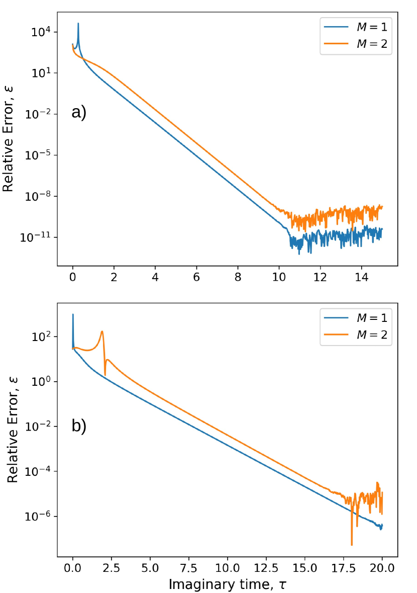
Figure 1: Relative error $\epsilon$ in $\Delta E$ computed via Eq. (3) plotted versus imaginary time $\tau$ for a) the 1D transverse field Ising and b) the Fermi Hubbard models with $M=1$ (blue) and $M=2$ (orange). We observe that in both models $\epsilon$ reaches a value of $10^{-4}$ or lower, which indicates that our method is able to accurately determine $\Delta E$. The negative linear trends in $\epsilon$ shown on these semilog plots are predicted by the error term in Eq. (3). The deviation from this trend at higher $\tau$ is an indication that the system has propagated in $\tau$ for too long and has lost information about the first excited state.

	$\Delta E_{\mathrm{exact}}$	$\Delta E_{\mathrm{method}}$	Relative Error
$E_{0}+E_{1}$	-10.05	-10.05	7.4 $\times 10^{-7}$
$E_{2}-E_{1}$	2.664	2.804	0.058
a) 1D Transverse Field Ising Model
	$\Delta E_{\mathrm{exact}}$	$\Delta E_{\mathrm{method}}$	Relative Error
$E_{0}+E_{1}$	-5.633	-5.632	1.7 $\times 10^{-4}$
$E_{2}-E_{1}$	-0.8363	-0.8504	0.017
b) 1D Fermi-Hubbard Model

Table 1: Relative error in using Eq. (9) and Eq. (10) to calculate $E_{0}+E_{1}$ and $E_{2}-E_{1}$ respectively with $M=1$. These results indicate that Eq. (9) can be used to accurately calculate $E_{0}+E_{1}$ and that Eq. (10) can be used to obtain an estimate for the second spectral gap.

III.1 Transverse Field Ising Model

We first demonstrate this method through numerical simulation of the 1D transverse field Ising model. This model has been widely studied in the contexts of quantum phase transitions [22, 23], quantum spin glasses [24, 25], and quantum annealing processes [26, 27, 28, 29]. Additionally, the 1D version of the model is known to be exactly solvable, which makes it a very useful numerical testing ground [30, 22]. This model consists of a lattice of spin states with nearest-neighbor interactions $J$ governed by the alignment of the spins, and its Hamiltonian is given by

$$H=-J\sum_{l=0}^{L-1}Z_{l}Z_{l+1}-h\sum_{l=0}^{L-1}X_{l},$$ (11)

where $Z_{l}$, $X_{l}$ denote Pauli $Z$ and $X$ matrices on site $l$, respectively, $h$ is the uniform magnetic field strength in the $z$-direction, and $L$ is the total number of lattice sites. Here we use periodic boundary conditions such that $\sigma_{L}=\sigma_{0}$. We choose the coordinating observable to be

$$O=-J(Z_{0}+Z_{1}),$$ (12)

which corresponds to the individual magnetization of spins on sites 1 and 2 scaled by $J$. To check the performance of the method, we plot the relative error

$$\epsilon=\frac{|\Delta E_{\mathrm{exact}}-\Delta E_{\mathrm{method}}|}{\Delta E_{\mathrm{exact}}},$$ (13)

as a function of $\tau$ for the transverse field Ising model with $J=1$, $L=4$, $h=1$ in Fig. 1a. In Eq. (13), $\Delta E_{\mathrm{exact}}$ is obtained via diagonalization of Eq. (11) and $\Delta E_{\mathrm{method}}$ is obtained using Eq. (3) with $M=1$ (blue) and $M=2$ (orange). In both cases, $\epsilon$ reaches approximately $10^{-8}$ or lower, which indicates that this method is able to accurately calculate the spectral gap for this system. Furthermore, the linear trend in the error on a log plot is predicted by the error term in Eq. (3) being exponential in $-\tau$. The change in the trend of the error above $\tau\approx 10$ is due primarily to the fact that the system has propagated too far in $\tau$ and thus lost the information about the first excited state.

We also check the performance of using Eq. (9) to calculate $E_{0}+E_{1}$ and Eq. (10) to calculate the second spectral gap $E_{2}-E_{1}$ by calculating the relative error of each. Here we use the same parameters for the transverse field Ising model as before, but only consider the $M=1$ case. These results are presented in Table  1a. As before, $\Delta E_{\mathrm{exact}}$ refers to the values for $E_{0}+E_{1}$ and $E_{2}-E_{1}$ obtained via diagonalization of Eq. (11), while $\Delta E_{\mathrm{method}}$ refers to the values obtained using Eq. (9) or (10). These results show that Eq. (9) can be used to accurately determine $E_{0}+E_{1}$. If $E_{0}$ or $E_{1}$ are known, this can be used to calculate the spectral gap without taking the ratio of potentially small numbers. These results also demonstrate that Eq. (10) can be used to estimate the second spectral gap once $\Delta E$ has been obtained.

III.2 Fermi-Hubbard

We next consider applications to the 1D Fermi-Hubbard model. This model describes strongly-correlated systems of fermions arranged on a lattice and has been used to describe transitions between conducting and insulating behavior [31], superconductivity [32], and magnetism [33]. The model Hamiltonian is

$$H =-t\sum_{l=0,\sigma}^{L-1}(c_{l\sigma}^{\dagger}c_{l+1,\sigma}-c_{l\sigma}c_{l+1,\sigma}^{\dagger})+U\sum_{l=0}^{L-1}n_{l\uparrow}n_{l\downarrow},$$ (14)

where $c_{l\sigma}^{\dagger},c_{l\sigma}$ are the fermionic creation and annihilation operators respectively at site $l$ with spin $\sigma$, $n_{l\sigma}=c_{l\sigma}^{\dagger}c_{l\sigma}$ is the occupation number operator, $t$ denotes the tunneling amplitude, and $U$ denotes the on-site interaction parameter. We choose

$$O=n_{0}+n_{1}$$ (15)

to be the coordinating observable, where $n_{l}=n_{l\uparrow}+n_{l\downarrow}$. As for the transverse field Ising model investigated in Sec. III.1, we demonstrate the effectiveness of the method by plotting the relative error $\epsilon$ as a function of imaginary time $\tau$, where the spectral gap $\Delta E$ is obtained by applying Eq. (3) to the Fermi-Hubbard model at half-filling with $t=1,L=4,U=\sqrt{2}$ for $M=1$ (blue) and $M=2$ (orange) in Fig. 1b. From this, we see that this method shows good agreement with the exact spectral gap obtained by diagonalizing Eq. (14) for both the $M=1$ and $M=2$ cases. Additionally, we see the same linear trend in the relative error as predicted by the order of the error in Eq. (3).

We again show the effectiveness of using Eq. (9) and Eq. (10) to obtain $E_{0}+E_{1}$ and $E_{2}-E_{1}$ respectively by calculating the relative error of each for the Fermi-Hubbard model described above with $M=1$. The results are presented in Table  1b. Again, the column labelled $\Delta E_{\mathrm{exact}}$ contains the exact values of $E_{0}+E_{1}$ and $E_{2}-E_{1}$ as calculated from the spectrum of Eq. (14), while $\Delta E_{\mathrm{method}}$ contains the values obtainued using Eq. (9) or Eq. (10). These results demonstrate that Eq. (9) is an accurate method for calculating $E_{0}+E_{1}$ and could thus be a suitable alternative to Eq. (3) for calculating the spectral gap. Likewise, we see that Eq. (10) can be used to estimate the second gap after using Eq. (3) to get $\Delta E$.

IV Conclusion

We have developed a general method for calculating the spectral gap that makes use of imaginary time propagation and requires only the estimation of expectation values of local observables (Sec. II). This method takes advantage of imaginary time propagation’s ability to select out the lower energy states of a system. We demonstrate the performance of this method via numerical simulation of paradigmatic model systems: the transverse field Ising model (Sec. III.1) and the Fermi-Hubbard model (Sec. III.2).

Appendix A Commutator Expansion

We wish to demonstrate via induction that the $M$-th nested commutator of two general operators $H$ and $O$ is given by [19]

$$[H,O]_{M}=\sum_{m=0}^{M}(-1)^{m}\binom{M}{m}H^{M-m}OH^{m},$$ (16)

for any whole number $M$. Consider $[H,O]=HO-OH$. This can also be written as

$$[H,O] =\sum_{m=0}^{M=1}(-1)^{m}\binom{M}{m}H^{1-m}OH^{m},$$ (17)

$$=HO-OH.$$ (18)

Suppose this is true for the $M$-th commutator. Now consider calculating the commutator of $H$ with the previous expression to obtain the $M+1$-th commutator. Then we would have

$$[H,O]_{M+1} =\sum_{m=0}^{M}(-1)^{m}\binom{M}{m}H^{M-m+1}OH^{m}+$$

$$\sum_{m^{\prime}=0}^{M}(-1)^{m^{\prime}+1}\binom{M}{m^{\prime}}H^{M-m^{\prime}}OH^{m^{\prime}+1}.$$ (19)

Terms where $m=m^{\prime}+1$ can be simplified, but this requires separating the $m=0$ and $m^{\prime}=M$ terms from the sums to obtain

$$[H,O]_{M+1} =H^{M+1}O+X+(-1)^{M+1}OH^{M+1},$$ (20)

where $X$ is the summation containing like terms,

$$X =\sum_{m^{\prime}=0}^{M-1}(-1)^{m^{\prime}+1}H^{M-m^{\prime}}OH^{m^{\prime}+1}$$

$$\left[\binom{M}{m^{\prime}+1}+\binom{M}{m^{\prime}}\right].$$ (21)

Taking advantage of the fact that $\binom{n}{k}=\binom{n-1}{k}+\binom{n-1}{k-1}$ and adjusting indices to be clearer yields

$$X =\sum_{k=1}^{M}(-1)^{k}\binom{M+1}{k}H^{M+1-k}OH^{k},$$ (22)

Combining everything in Eq. (19), we have

$$[H,O]_{M+1} =H^{M+1}O$$

$$+\sum_{k=1}^{M}(-1)^{k}\binom{M+1}{k}H^{M+1-k}OH^{k}$$

$$+(-1)^{M+1}OH^{M+1},$$ (23)

or

$$[H,O]_{M+1} =\sum_{k=0}^{M+1}(-1)^{k}\binom{M+1}{k}H^{M+1-k}OH^{k}.$$ (24)

Thus, by induction, the expansion of the $M$-th order commutator is given by Eq. (16) for any $M$.