Composite Classical and Quantum Channel Discrimination

Abstract

We study the problem of binary composite channel discrimination in the asymmetric setting, where the hypotheses are given by fairly arbitrary sets of channels, and samples do not have to be identically distributed. In the case of quantum channels we prove: $(i)$ a characterization of the Stein exponent for parallel channel discrimination strategies and $(ii)$ an upper bound on the Stein exponent for adaptive channel discrimination strategies. We further show that already for classical channels this upper bound can sometimes be achieved and be strictly larger than what is possible with parallel strategies. Hence, there can be an advantage of adaptive channel discrimination strategies with composite hypotheses for classical channels, unlike in the case of simple hypotheses. Moreover, we show that classically this advantage can only exist if the sets of channels corresponding to the hypotheses are non-convex. As a consequence of our more general treatment, which is not limited to the composite i.i.d. setting, we also obtain a generalization of previous composite state discrimination results.

1 Introduction and Outline

Hypothesis testing, or finding optimal strategies and minimal errors for discrimination tasks is one of the oldest and most studied tasks in information theory. In the quantum setting there have been plenty of results regarding the optimal discrimination of states [helstrom_quantum_1976, Kho79, HP91, ON00, Nag06, Aud+07, Hay07, Aud+08, NS09, AMV12, BK15, mosonyi_error_2021] and also quantum channels [CDP08, DFY09, Hay09, Har+10, WW19, Fan+20, Wil+20]. However, most of the quantum literature focuses on the case where the two hypotheses are simple, i.e. the hypotheses state that what we are given is exactly one specific state (or channel). Arguably, much more practically relevant is the case where one allows for composite hypotheses, i.e. hypotheses stating that the given state (or channel) belongs to a certain set. This first of all includes the noisy regime, where we can assume that what we are given is approximately one of two possibilities, but also much more general settings, i.e. questions of discriminating big sets with a certain structure (for states this could for example be sets of separable [Bra+20] or coherent [BBH21] states).

Throughout this paper we will be looking at binary composite hypothesis testing in the asymmetric setting. We are given $n$ instances of an unknown object, and have to make a decision between two hypotheses based on these $n$ instances, and are ultimately interested in the asymptotic limit $n\to\infty$. We will start with introducing the problem for discriminating two sets of states, and give an overview of previous results in the literature, before moving on to the problem of discriminating two sets of channels. To our knowledge, the task of composite binary quantum channel discrimination has not been studied thus far. Throughout our analysis, we will not restrict ourselves to the composite i.i.d. setting, i.e. we will also allow the provided objects (states or channels) to vary within the sets corresponding to the hypotheses.

For binary asymmetric composite channel discrimination we show in this fairly general setting: $(i)$ a characterization of the Stein exponent for parallel channel discrimination strategies (Theorem 9), and $(ii)$ an upper bound on the Stein exponent for adaptive channel discrimination strategies (10). We further show that already classically this upper bound can sometimes be achieved and be strictly larger than what is possible with parallel strategies (12), and hence there can be an advantage of adaptive channel discrimination strategies with composite hypotheses. We go on to show that classically this advantage can only exist if the sets of channels corresponding to the hypotheses are non-convex, and additionally assuming this convexity makes parallel strategies asymptotically optimal (Theorem 13). We leave the question open whether an adaptive advantage can exist in the quantum case when the sets of channels are convex. Table 1 gives an overview of what we are able to show regarding composite channel discrimination, and illustrates in which cases an adaptive advantage exists.

As a consequence of our more general treatment which is not limited to the composite i.i.d. setting we also obtain a generalization of the composite state discrimination results of [BBH21] (Theorem 5). Note, however, that while we do not require provided states or channels to be identical, we still require them to be independent. Hence, our theorems do not aid in determining whether a generalized Stein’s lemma holds in cases where the alternative hypothesis is given by a set of non-independent states, as conjectured in [BP10, Ber+22a].

Summary of Main Results

Hypotheses	Asymptotic Parallel Exponent		Asymptotic Adaptive Exponent		Upper Bound	Shown in
Quantum Simple	$D_{\mathrm{reg}}(\mathcal{E}\|\mathcal{F})$	$=$	$D_{A}(\mathcal{E}\|\mathcal{F})$			[WW19] [Wil+20] [Fan+20]
Classical Composite Convex Sets	$\displaystyle\max_{\nu}\min_{\begin{subarray}{c}\mathcal{E}\in\mathcal{S}\\ \mathcal{F}\in\mathcal{T}\end{subarray}}D(\mathcal{E}(\nu)\|\mathcal{F}(\nu))$	$=$	$\displaystyle\min_{\begin{subarray}{c}\mathcal{E}\in\mathcal{S}\\ \mathcal{F}\in\mathcal{T}\end{subarray}}D(\mathcal{E}\|\mathcal{F})$	$=$	$\displaystyle\min_{\begin{subarray}{c}\mathcal{E}\in\mathcal{S}\\ \mathcal{F}\in\mathcal{T}\end{subarray}}D(\mathcal{E}\|\mathcal{F})$	Thm. 13
Classical Composite Finite Sets	$\displaystyle\max_{\nu}\min_{\begin{subarray}{c}\mathcal{E}\in\mathcal{S}\\ \mathcal{F}\in\mathcal{T}\end{subarray}}D(\mathcal{E}(\nu)\|\mathcal{F}(\nu))$	$<$ i.g.	$?$	$\leq$	$\displaystyle\min_{\begin{subarray}{c}\mathcal{E}\in\mathcal{S}\\ \mathcal{F}\in\mathcal{T}\end{subarray}}D(\mathcal{E}\|\mathcal{F})$	Prop. 14 Ex. 12 Prop. 10
Quantum Composite	$\displaystyle\lim_{n\to\infty}{1\over n}\min_{\begin{subarray}{c}\mathcal{E}_{n}\in\mathcal{C}(\mathcal{S}_{n})\\ \mathcal{F}_{n}\in\mathcal{C}(\mathcal{T}_{n})\end{subarray}}D(\mathcal{E}_{n}\|\mathcal{F}_{n})$	$<$ i.g.	$?$	$<$ i.g.	$\displaystyle\min_{\begin{subarray}{c}\mathcal{E}\in\mathcal{S}\\ \mathcal{F}\in\mathcal{T}\end{subarray}}D_{A}(\mathcal{E}\|\mathcal{F})$	Thm. 9 Ex. 12 Prop. 10 Rem. 11

Table 1: Illustration of the relation between adaptive and parallel type II error exponents for various channel discrimination tasks. For the composite problems the task is to discriminate between two sets of channels $\mathcal{S}$ and $\mathcal{T}$ and the table also includes an upper bound based on the worst-case simple i.i.d. problem. “Quantum Simple” refers to the quantum channel discrimination problem with simple hypotheses. With “Classical” we mean that all channels are classical, and “Convex Sets” or “Finite Sets” refers to whether the sets of channels $\mathcal{S}$ and $\mathcal{T}$ are convex or finite. Please see the respective theorems for a general formulation of the results and a precise definition of the quantities involved; $\mathcal{C}$ denotes the convex hull. We write i.g. to denote that these inequalities will be strict in general, although there exist specific examples where equality holds.

2 Mathematical Preliminaries

We write $\mathcal{H}$ for a complex finite-dimensional Hilbert space, and $\mathcal{B}\left(\mathcal{H}\right)$ for the set of linear operators acting on $\mathcal{H}$. We write $\mathscr{P}\left(\mathcal{H}\right)$ for the set of positive semi-definite operators acting on $\mathcal{H}$. For $A,B\in\mathscr{P}\left(\mathcal{H}\right)$, we further write $A\ll B$ if $\textrm{supp}\left(A\right)\subseteq\textrm{supp}\left(B\right)$ and $A\not\ll B$ if $\textrm{supp}\left(A\right)\not\subseteq\textrm{supp}\left(B\right)$. Let $\mathcal{D}\left(\mathcal{H}\right)$ denote the set of density matrices, i.e., the set of positive semi-definite operators with trace one. A quantum channel (in this paper usually denoted as $\mathcal{E}$ or $\mathcal{F}$) is a completely positive trace preserving map between density operators. We will label different quantum systems by capital Roman letters ($A$, $B$, $C$, etc.) and often use these letters interchangeably with the corresponding Hilbert space or set of density matrices (i.e., we write $\rho\in\mathcal{D}\left(A\right)$ instead of $\rho\in\mathcal{D}\left(\mathcal{H}_{A}\right)$ and $\mathcal{E}:A\to B$ instead of $\mathcal{E}:\mathcal{D}\left(\mathcal{H}_{A}\right)\to\mathcal{D}\left(\mathcal{H}_{B}\right)$). We will also concatenate these letters to mean tensor products of systems, i.e. we will write $\rho\in\mathcal{D}\left(RA\right)$ for $\rho\in\mathcal{D}\left(\mathcal{H}_{R}\otimes\mathcal{H}_{A}\right)$. We write $\mathrm{CPTP}(A\to B)$ for the set of all completely positive trace preserving maps from $\mathcal{D}\left(\mathcal{H}_{A}\right)$ to $\mathcal{D}\left(\mathcal{H}_{B}\right)$. Throughout the paper we will write $\mathcal{X}$ and $\mathcal{Y}$ for classical systems. A classical state $\rho\in\mathcal{D}\left(\mathcal{X}\right)$ is then diagonal in the computational basis, and we write $\mathrm{CPTP}(\mathcal{X}\to\mathcal{Y})$ for the set of classical channels.

For any subset $A$ of a vector space, we will write $\mathcal{C}(A)$ for the convex hull of $A$. We write $\log$ for the logarithm to the base two.

2.1 Measurements and POVMs

Throughout this paper we will treat measurements and POVMs as quantum-classical channels, i.e. we associate a POVM specified through the operators $\{M_{i}\}_{i=1}^{n}\subset\mathcal{B}\left(\mathcal{H}\right)$ with the quantum-classical channel

$$\mathcal{M}:\mathcal{D}\left(\mathcal{H}\right)\to\mathcal{D}\left(\mathbb{C}^{n}\right)\qquad\rho\mapsto\sum_{i=1}^{n}\Tr(\rho M_{i})\outerproduct{i}{i}\,.$$ (1)

2.2 Quantum Information Measures

For $\rho\in\mathcal{D}\left(\mathcal{H}\right)$ and $\sigma\in\mathscr{P}\left(\mathcal{H}\right)$ the (Umegaki) quantum relative entropy is defined as [Ume62]

$$D(\rho\|\sigma)\coloneqq\Tr(\rho(\log\rho-\log\sigma)),$$ (2)

if $\rho\ll\sigma$ and $D(\rho\|\sigma)\coloneqq\infty$ if $\rho\not\ll\sigma$. One of its most important properties is the data-processing inequality [Lin75], which states that for every quantum channel $\mathcal{E}$:

$$D(\rho\|\sigma)\geq D(\mathcal{E}(\rho)\|\mathcal{E}(\sigma))\,.$$ (3)

A self-contained proof can be found e.g. in [KW20]. More generally, we call a function of $\rho$ and $\sigma$ a divergence if it satisfies the data-processing inequality.

We can also define the measured relative entropy as the maximal classical relative entropy when measuring both states with some POVM. Specifically

$$D_{M}(\rho\|\sigma)\coloneqq\sup_{\mathcal{M}\text{ POVM}}D(\mathcal{M}(\rho)\|\mathcal{M}(\sigma))$$ (4)

where $\mathcal{M}$ is a POVM (with arbitrary many outcomes) interpreted as a quantum-classical channel as outlined above.

For $\rho\in\mathcal{D}\left(\mathcal{H}\right)$ and $\sigma\in\mathscr{P}\left(\mathcal{H}\right)$, define the quantum max-divergence (or the max-relative entropy) as [Dat09]

$$D_{\max}(\rho\|\sigma)\coloneqq\log\inf\Set{\lambda\in\mathbb{R}}{\rho\leq\lambda\sigma}\,.$$ (5)

The quantum max-divergence also satisfies the data-processing inequality [Dat09].

We will also frequently use the hypothesis testing relative entropy, which for $\rho,\sigma\in\mathcal{D}\left(\mathcal{H}\right)$ is defined as follows [WR12]

$$D_{H}^{\varepsilon}(\rho\|\sigma)\coloneqq\min_{\begin{subarray}{c}0\leq M\leq\IdentityMatrix_{\mathcal{H}}\\ \Tr(M\rho)\geq 1-\varepsilon\end{subarray}}\Tr(\sigma M)\,.$$ (6)

2.2.1 Channel Divergences

For every given divergence $\mathbf{D}$ for states, one can define an associated channel divergence [Led+18] by performing a (stabilized) maximization over all input states, i.e. with $\mathcal{E},\mathcal{F}:A\to B$ being quantum channels

$$\mathbf{D}(\mathcal{E}\|\mathcal{F})\coloneqq\sup_{\rho_{RA}\in\mathcal{D}\left(R\otimes A\right)}\mathbf{D}\big{(}(\textrm{id}_{R}\otimes\mathcal{E})(\rho)\|(\textrm{id}_{R}\otimes\mathcal{F})(\rho)\big{)}.$$ (7)

Since $\mathbf{D}$ satisfies the data-processing inequality by definition, the supremum can be restricted to pure states such that the reference system $R$ is isomorphic to the channel input system $A$ (this is shown below as 17).

For the Umegaki relative entropy $D$, we can also define the regularized and amortized [Wil+20] channel divergences as

$$D_{\mathrm{reg}}(\mathcal{E}\|\mathcal{F}) \coloneqq\lim_{n\to\infty}{1\over n}\mathbf{D}(\mathcal{E}^{\otimes n}\|\mathcal{F}^{\otimes n}),$$ (8)

$$D_{A}(\mathcal{E}\|\mathcal{F}) \coloneqq\sup_{\begin{subarray}{c}\rho,\sigma\in\mathcal{D}\left(RA\right)\\ R\text{ arbitrary}\end{subarray}}\quantity[\mathbf{D}(\mathcal{E}(\rho)\|\mathcal{F}(\sigma))-\mathbf{D}(\rho\|\sigma)].$$ (9)

Note that for the amortized divergence, there is no known way in which the size of the reference system can be restricted.

3 Composite State Discrimination

In simple quantum state discrimination, given $n$ identical copies of an unknown state which is promised to be either $\rho$ or $\sigma$, the task is to decide which of the two options it is. In composite quantum state discrimination, we are only promised that the states are all from one of two sets $S$ or $T$, and the task is to decide which set they come from (but not to further identify which state exactly was provided). Since there are now multiple states for each hypothesis, there are multiple possible scenarios how the $n$ input states one receives are related: We could still be given $n$ identical copies of a state, or alternatively, we could be given $n$ completely different states but all from the same set $S$ or $T$, or something in between, where the states are non-identical but still related. We would like to cover all these different scenarios in our analysis, and hence we will describe composite hypotheses as sequences of sets $S_{n}$ which include all the possible combinations of $n$ states we could get. We will make some small assumptions on these sets:

Definition 1.

For the purpose of this work, a composite quantum state hypothesis (in the asymptotic setting) is a sequence of sets of states

$$\bm{S}=(S_{n}\subset\mathcal{D}\left(\mathcal{H}^{\otimes n}\right))_{n}$$

such that

1. Each set $S_{n}$ is topologically closed.

2. Each element $\rho_{n}\in S_{n}$ is a tensor product of states $\rho_{n}=\rho^{(1)}\otimes\ldots\otimes\rho^{(n)}$, with each $\rho^{(i)}\in\mathcal{D}\left(\mathcal{H}\right)$ for $i=1,...,n$.

3. The sets $S_{n}$ are closed under tracing out any subsystem, i.e. for any $i=1,...,n$ and $\rho_{n}\in\mathcal{S}_{n}$ we have that $\Tr_{i}(\rho_{n})\in\mathcal{S}_{n-1}$, where $\Tr_{i}$ denotes the partial trace over the $i^{th}$ subsystem.

4. Each set $S_{n}$ is closed under permutation of the $n$ subsystems, i.e. for any permutation $\pi\in S(n)$ and associated canonical unitary representation $\Pi$, we have for all $\rho_{n}\in S_{n}$: $\Pi\rho_{n}\Pi\in\mathcal{S}_{n}$.

Interesting examples of this include:

1. The composite i.i.d. case: We have two sets $S$, $T\subset\mathcal{D}\left(\mathcal{H}\right)$, and are given $n$ identical copies of an element from $S$ if the null hypothesis is true, and $n$ identical copies of an element from $T$ if the alternate hypothesis is true. This corresponds to:

   $$S_{n} \coloneqq\Set{\rho^{\otimes n}}{\rho\in S},$$ (10)

   $$T_{n} \coloneqq\Set{\sigma^{\otimes n}}{\sigma\in T}.$$ (11)

2. The arbitrarily varying case: This is similar to the composite i.i.d. case, but we are not given $n$ identical copies, but $n$ (potentially different) elements from $S$ or $T$. This corresponds to:

   $$S_{n} \coloneqq\Set{\rho_{1}\otimes\ldots\otimes\rho_{n}}{\rho_{1},\ldots\rho_{n}\in S},$$ (12)

   $$T_{n} \coloneqq\Set{\sigma_{1}\otimes\ldots\otimes\sigma_{n}}{\sigma_{1},\ldots\sigma_{n}\in T}.$$ (13)

3. The slightly-varying case: This is an example of a scenario that lies in between the arbitrarily varying case (where there is no correlation between the samples, except for them all being in the same set) and the composite i.i.d. case (where there is maximal correlation between the samples, as they are all identical). For any given $\varepsilon\in[0,1]$ (which might depend on $n$) and any distance function $d:\mathcal{D}\left(\mathcal{H}\right)\crossproduct\mathcal{D}\left(\mathcal{H}\right)\to[0,1]$ (e.g.  trace distance or purified distance) set

   $$S_{n} \coloneqq\Set{\rho_{1}\otimes\ldots\otimes\rho_{n}}{\rho_{1},\ldots\rho_{n}\in S,\quad d(\rho_{i},\rho_{j})\leq\varepsilon\;\forall i,j},$$ (14)

   $$T_{n} \coloneqq\Set{\sigma_{1}\otimes\ldots\otimes\sigma_{n}}{\sigma_{1},\ldots\sigma_{n}\in T,\quad d(\sigma_{i},\sigma_{j})\leq\varepsilon\;\forall i,j}.$$ (15)

4. The simple i.i.d. case: The simple i.i.d. case can be seen as a special case of the above where $S$ and $T$ each contain one element.

Lemma 2.

If $\bm{S}$ is a quantum state hypothesis, then performing a measurement on any (joint) $k$ subsystems of a state $\rho_{n}\in S_{n}$, and conditioning on the measurement result, yields a state $\rho_{n-k}$ on the remaining subsystems that is an element of $S_{n-k}$. Precisely, let $k\in\{1,...,n\}$, $\rho_{n}\in S_{n}\subset\mathcal{D}\left(\mathcal{H}^{\otimes n}\right)$ and $0\leq M\leq\IdentityMatrix\in\mathcal{B}\left(\mathcal{H}^{\otimes k}\right)$. If

$$\omega_{n-k}\coloneqq\Tr_{1,...,k}\quantity[(M\otimes\IdentityMatrix_{\mathcal{H}_{k+1}}\otimes...\otimes\IdentityMatrix_{\mathcal{H}_{n}})\rho_{n}]$$ (16)

then either $\Tr(\omega_{n-k})=0$ or $\omega_{n-k}/\Tr(\omega_{n-k})\in S_{n-k}$.

Proof.

This follows immediately from the fact that each element $\rho_{n}\in S_{n}$ is a tensor product, and that removing an element in the tensor product gives an element in $S_{n-1}$. ∎

Remark 3.

Note that while we state the results below with the assumptions of 1, we could replace the required tensor product structure (point 2 in 1) with the statement of 2. While this might be more general, we find the assumptions of 1 to be more natural. Similarly, later on when talking about hypotheses in the context of channel discrimination, we could replace the tensor product structure for channels in (point 2 in 8) with the statement of 2 for any tensor product input state.

For our discrimination problem, given an $n$ and an unknown state in $\mathcal{D}\left(\mathcal{H}^{\otimes n}\right)$ we will want to perform a binary POVM (fully specified by one of its elements, which we write as $M$) to decide between the two hypotheses. In the end we want to avoid making an error, i.e. claiming that our state comes from $S_{n}$ when it actually comes from $T_{n}$ and vice-versa. These two errors are known as type I and type II errors. If we settle on a measurement $M$, the probability of making an error might still depend on which particular state from either $S_{n}$ or $T_{n}$ we actually end up getting. Here we will be focussing on minimizing the worst case errors, i.e. we want to choose measurements which minimize the error uniformly over all states from $S_{n}$ and $T_{n}$. More formally, we define the type I and type II error probabilities (also called type I and type II errors) as:

$$\alpha(M,S_{n}) =\sup_{\rho\in S_{n}}\Tr((\IdentityMatrix-M)\rho)$$ (17)

$$\beta(M,T_{n}) =\sup_{\sigma\in T_{n}}\Tr(M\sigma)\,.$$ (18)

We will be focussing on the asymmetric setting, where we want to minimize the type II error, $\beta$, under the constraint that the type I error $\alpha$ is below a certain threshold. The main quantity of interest is then the negative logarithm of this minimal type II error under the type I error constraint, which we also call the hypothesis testing relative entropy of the two sets $S_{n}$ and $T_{n}$:

$$D_{H}^{\varepsilon}(S_{n}\|T_{n})\coloneqq-\inf_{\begin{subarray}{c}0\leq M\leq\IdentityMatrix\\ \alpha(M,S_{n})\leq\varepsilon\end{subarray}}\log\beta(M,T_{n})\,.$$ (19)

As the expression in (17) is linear in $\rho$, it is easy to see that

$$\alpha(M,\mathcal{C}(S_{n}))=\alpha(M,S_{n})$$ (20)

(remember that $\mathcal{C}$ is the convex hull) as the supremum will be achieved at an extremal point, and the same holds also for $\beta$.

Hence,

$$D_{H}^{\varepsilon}(S_{n}\|T_{n})=D_{H}^{\varepsilon}(S_{n}\|\mathcal{C}(T_{n}))=D_{H}^{\varepsilon}(\mathcal{C}(S_{n})\|T_{n})=D_{H}^{\varepsilon}(\mathcal{C}(S_{n})\|\mathcal{C}(T_{n}))$$ (21)

and hence the discrimination task considered is equivalent to discriminating between these convex hulls of the sets $S_{n}$ and $T_{n}$. We are interested in the quantum Stein exponent for this discrimination task, i.e. the optimal exponential decay rate of the type II error in the limit of infinitely many copies of the state, given that the type I error also goes to zero asymptotically. This Stein exponent can be expressed as

$$\lim_{\varepsilon\to 0}\lim_{n\to\infty}\frac{1}{n}D^{\varepsilon}_{H}(S_{n}\|T_{n})\,.$$ (22)

In [BBH21], this problem was studied specifically in the composite i.i.d. case, i.e. with $S_{n}=\Set{\rho^{\otimes n}}{\rho\in S}$, $T_{n}=\Set{\sigma^{\otimes n}}{\sigma\in T}$, where $S,T\subset\mathcal{D}\left(\mathcal{H}\right)$ were also assumed to be closed and convex, leading to:

Theorem 4 ([BBH21]).

Let $S,T$ be closed and convex, and define for all $n$: $S_{n}\coloneqq\Set{\rho^{\otimes n}}{\rho\in S}$, $T_{n}\coloneqq\Set{\sigma^{\otimes n}}{\sigma\in T}$. Then

$$\lim_{\varepsilon\to 0}\lim_{n\to\infty}\frac{1}{n}D^{\varepsilon}_{H}(S_{n}\|T_{n})=\lim_{n\to\infty}\frac{1}{n}\inf_{\begin{subarray}{c}\rho_{n}\in\mathcal{S}_{n}\\ \sigma_{n}\in\mathcal{C}(T_{n})\end{subarray}}D(\rho_{n}\|\sigma_{n})\,,$$ (23)

and one can find cases where this is strictly smaller than

$$\inf_{\begin{subarray}{c}\rho\in S\\ \sigma\in T\end{subarray}}D(\rho\|\sigma)\,.$$ (24)

Remember that $\mathcal{C}$ stands for the convex hull, and it is precisely this convex hull in the infimum on the right-hand side of (23) which prevents the regularization from collapsing, as the elements of $S_{n}$ and $T_{n}$ are tensor products, and the relative entropy is additive. Without this convex hull, the exponent (23) would be exactly equal to the single-letter expression (24), which we call the worst-case i.i.d. exponent, as it is equal to the exponent of the worst-case simple i.i.d. problem. Intuitively, one pays for the compositeness by having to include convex combinations in the Stein exponent, and this makes the discrimination problem strictly harder in some cases.

As a consequence of our channel discrimination result further below (Theorem 9), we will arrive at this following generalization of Theorem 4:

Theorem 5.

Let $\bm{S}=(S_{n})_{n},\bm{T}=(T_{n})_{n}$ be two composite quantum state hypotheses. Then

$$\lim_{\varepsilon\to 0}\lim_{n\to\infty}\frac{1}{n}D_{H}^{\varepsilon}(S_{n}\|T_{n})=\lim_{n\to\infty}\frac{1}{n}\min_{\begin{subarray}{c}\rho_{n}\in\mathcal{C}(\mathcal{S}_{n})\\ \sigma_{n}\in\mathcal{C}(T_{n})\end{subarray}}D(\rho_{n}\|\sigma_{n})\,,$$ (25)

Furthermore, if each $S_{n}$ lies in a linear subspace of $\mathcal{D}\left(\mathcal{H}^{\otimes n}\right)$ with dimension polynomial in $n$ (this holds for example in the composite i.i.d. case, where each $\rho_{n}\in S_{n}$ is permutation invariant), then we can remove the first convex hull to get

$$\lim_{\varepsilon\to 0}\lim_{n\to\infty}\frac{1}{n}D^{\varepsilon}_{H}(S_{n}\|T_{n})=\lim_{n\to\infty}\frac{1}{n}\min_{\begin{subarray}{c}\rho_{n}\in\mathcal{S}_{n}\\ \sigma_{n}\in\mathcal{C}(T_{n})\end{subarray}}D(\rho_{n}\|\sigma_{n})\,.$$ (26)

Proof.

This follows as a special case of Theorem 9 below. ∎

Remark 6.

Our Theorem 5 generalizes the previous Theorem 4 in multiple ways: Already in the composite i.i.d. setting it no longer requires the sets $\mathcal{S}$ and $\mathcal{T}$ to be convex. Additionally our theorem also includes all the non-i.i.d. cases such as the arbitrarily (or slightly varying) cases defined above.

3.1 Classical Adversarial Hypothesis Testing

Similar to [Bra+20, BBH21] our results are based on a reduction to a classical problem, the one of adversarial hypothesis testing. The following is a brief recapitulation of the treatment of adversarial hypothesis testing in [Bra+20]. Let $P,Q\subset\mathbb{R}^{\Omega}$ (for a finite domain $\Omega$) be two sets of probability distributions. In the typical composite i.i.d. setting, we are presented with $n$ samples from a distribution in $P$ or $Q$ and have to make a decision which set the distribution comes from. In the adversarial setting, the adversary is allowed to change the distribution within $P$ or $Q$ for each sample, and he can make this change based on the samples we observed previously. Note that while the adversary has access to the previous samples, he can only select a probability distribution $p\in P$ or $q\in Q$ (depending on which hypothesis is true) for the next sample, but he cannot select the sample outcome itself. The adversary is fully specified by two sets of functions $\hat{p}_{k}:\Omega^{k-1}\to P$ and $\hat{q}_{k}:\Omega^{k-1}\to Q$, which for each $k$ specify how the adversary picks the next probability distribution based on the previous $k-1$ sample outcomes ($\hat{p}_{k}$ is used if the null hypothesis is true, and $\hat{q}_{k}$ is used if the alternate hypothesis is true). The probability of a sample string $\mathbf{x}\in\Omega^{n}$ is then given by

$$\hat{p}(\mathbf{x})\coloneqq\prod_{k=1}^{n}\hat{p}_{k}(x_{1},\ldots,x_{k-1})(x_{k})$$ (27)

For any decision region $A_{n}\subset\Omega^{n}$, the type I and type II errors are then going to be the worst-case errors over all adversarial strategies. We define the corresponding $n$-shot error exponent as

$$D_{\textrm{adv},n}^{\varepsilon}(P\|Q)=-\log\inf\Set{\sup_{\hat{q}}\hat{q}(A_{n})}{A_{n}\subset\Omega^{n},\;\sup_{\hat{p}}\hat{p}(A_{n}^{c})\leq\varepsilon}$$ (28)

The key statement of [Bra+20] is that if the sets $P$ and $Q$ are closed and convex, adversarial hypothesis testing is asymptotically no harder than the worst-case i.i.d. setting, specifically:

Theorem 7 ([Bra+20, Theorem 2]).

Let $\Omega$ be a finite domain and $P,Q\subset\mathbb{R}^{\Omega}$ be two closed, convex sets of probability distributions. Then, for any $\varepsilon\in(0,1)$:

$$\lim_{n\to\infty}{1\over n}D_{\mathrm{adv},n}^{\varepsilon}(P\|Q)=\min_{p\in P,q\in Q}D(p\|q)$$ (29)

Note that since we are taking the supremum over all adversaries, by picking an adversary that deterministically picks states in a certain sequence, this result implies that also any composite problem is classically asymptotically equally as hard as the worst-case i.i.d. problem (it is also easy to see that the composite problem cannot be simpler than the worst-case i.i.d. problem).

4 Composite Channel Discrimination

The task of composite channel discrimination is very similar in nature to composite state discrimination, but also considerably harder to study: Given an unknown quantum channel as a black box and the side information that it comes from two sets of possible channels, the task is again to determine the set (but not necessarily the exact identity) of the channel. The additional complexity here comes from the fact that, on top of finding the best measurement to perform on the output of the channel, we also have to figure out which quantum states to send as inputs to the channel.

If we are given access to the black box multiple times (or say we are given multiple black-boxes) the problem becomes considerably more interesting, as the channel inputs could be chosen based on previous channel outputs. Say we are given access to $n$ black-boxes (we will allow for the case where not all black-boxes are identical and will specify further below what scenarios exactly we consider, intuitively though the scenario is always that we want to distinguish $n$ black-boxes from one set to $n$ black-boxes from another set). There are now different strategies (sometimes also called protocols) in which we could set up our decision experiment – the so-called parallel and adaptive strategies.

In a parallel strategy one prepares a joint state, usually entangled between the input systems of all the $n$ channels and an additional reference (or memory) system. This state is then fed as input to all the $n$ channels at once (with the state of the reference system being left undisturbed). Finally, a binary positive operator-valued measure (POVM) is performed on the joint state at the output of the channels and the reference system in order to arrive at a decision. In an adaptive strategy, on the other hand, one prepares a state of the input system of a single channel (again usually entangled with a reference system) which is fed into the first channel, with the state of the reference system being left undisturbed. The input to the next use of the channel is then chosen depending on the output of the first channel and the state of our reference system. This is done, most generally, by subjecting the latter to an arbitrary quantum operation (or channel), which we call a preparation operation. This step is repeated for each successive black-box channel until all the $n$ black-boxes have been used. Then a binary POVM is performed on the joint state of the output of the last use of the channel and the reference system. See Figure 1 for a depiction of an adaptive strategy. Adaptive strategies are also sometimes called sequential, which is, however, not to be confused with the setting of sequential hypothesis testing [Mar+21, LTT22, LHT22], where samples (i.e. states or channels) can be requested one by one.

One particularly interesting question is whether and to what degree adaptive strategies give an advantage over parallel ones. Note that any parallel strategy can be written as an adaptive strategy by taking all but one channel input as part of the reference system, and then choosing each preparation operation such that it extracts the next part of the joint input state for the next channel use and replaces it by the output of the previous channel use. However, the converse is not true, and so adaptive strategies are more general. Parallel strategies are conceptually a lot simpler than adaptive ones – aside from the measurement, everything is specified just by the joint input state – in contrast to adaptive strategies, in which after each channel use we can perform an arbitrary quantum operation to prepare the input to the next use of the channel. It is thus interesting to determine to what degree parallel strategies can still be optimal.

This problem has been studied extensively for channel discrimination with simple hypotheses, where it is known that in certain cases adaptive strategies can give an advantage over parallel ones. In [Har+10] the authors constructed an example in which an adaptive strategy with only two channel uses could be used to discriminate two channels with certainty, which is shown not to be possible with a parallel strategy, even if arbitrarily many channel uses are allowed. Asymptotically, however, it was shown that in the simple binary asymmetric case adaptive and parallel strategies are equivalent [WW19, Fan+20, Wil+20]. We will show below that this fails to stay the case with composite hypotheses, already classically.

Specifically, in this section we will study the following: 1. We start with a treatment of parallel channel discrimination strategies, where we provide matching achievability and converse bounds for the Stein exponent in terms of a regularized expression (Theorem 9), in analogy to what has previously been shown [BBH21] for state discrimination (i.e. Theorem 4). 2. We prove an upper bound on the Stein exponent for adaptive strategies (10), where we show that this upper bound can sometimes but not always be achieved, and can also be larger than the parallel exponent (12), hence demonstrating that adaptive strategies can sometimes be advantageous (we show this even classically). 3. We show that classically, under an additional convexity assumption which was not satisfied in the previous example, parallel and adaptive strategies are asymptotically equivalent in the asymmetric composite setting, and the Stein exponent is given by a single-letter entropic formula (Theorem 13). 4. We further show classically, and in some further restricted setting, that if we replace the convexity assumption with a finiteness assumption, we can still get a single-letter entropic expression for the Stein exponent for parallel strategies (14).

Following the above discussion for composite state discrimination, we want to apply a similar level of generality to discriminating channels, where we want to allow the $n$ black-boxes not be identical. Hence, in analogy with 1 we will work with general hypotheses satisfying the following conditions:

Definition 8.

For the purpose of this work, a composite quantum channel hypothesis (in the asymptotic setting) is a sequence of sets of channels

$$\bm{\mathcal{S}}=(\mathcal{S}_{n}\subset\mathrm{CPTP}(A^{n}\to B^{n}))_{n}$$

such that

1. Each set $\mathcal{S}_{n}$ is topologically closed.

2. Each element $\mathcal{E}_{n}\in\mathcal{S}_{n}$ is a tensor product of channels $\mathcal{E}_{n}=\mathcal{E}^{(1)}\otimes\ldots\otimes\mathcal{E}^{(n)}$, with $\mathcal{E}^{(i)}\in\mathrm{CPTP}(A\to B)$, for $i=1,...,n$.

3. For every $\mathcal{E}_{n}=\mathcal{E}^{(1)}\otimes\ldots\otimes\mathcal{E}^{(n)}\in\mathcal{S}_{n}$, removing any element in the tensor product yields an element in $\mathcal{S}_{n-1}$.

4. Each set $\mathcal{S}_{n}$ is closed under permuting the $n$ subsystems of the input and output systems of a channel, i.e. for any permutation $\pi\in S(n)$ and associated canonical unitary representations $\Pi_{A}$ and $\Pi_{B}$ on $A^{n}$ and $B^{n}$, we have for all $\mathcal{E}_{n}\in\mathcal{S}_{n}$ that also the permuted channel $\rho\mapsto\Pi_{B}\mathcal{E}_{n}(\Pi_{A}\rho\Pi_{A})\Pi_{B}$ is an element of $\mathcal{S}_{n}$.

One can then define the same scenarios, such as the composite i.i.d. setting, the arbitrarily varying setting, and slightly varying settings, as we did for composite state discrimination in a completely analogous way for composite channel discrimination.

4.1 The Parallel Case

Given a set of channels $\mathcal{A}$ and an input state $\nu\in\mathcal{D}\left(RA\right)$ (where $R$ could be any system, possibly also just trivial), we define the set of all output states as

$$\mathcal{A}[\nu]\coloneqq\Set{(\textrm{id}_{R}\otimes\mathcal{E})(\nu)}{\mathcal{E}\in\mathcal{A}}\,.$$ (30)

Similar to the state discrimination problem above, we will be looking for the best input state $\nu_{n}$ and measurement $M$ such that for all $\mathcal{E}_{n}\in\mathcal{S}_{n}$ the error of claiming it coming from $\mathcal{T}_{n}$ (i.e. the type I error) stays below some threshold $\varepsilon$ and we otherwise minimize the worst case type II error, i.e. we want to make sure that the probability of claiming an element $\mathcal{F}_{n}\in\mathcal{T}_{n}$ to be from $\mathcal{S}_{n}$ is as low as possible uniformly over all $\mathcal{F}_{n}\in\mathcal{T}_{n}$. Given an input state $\nu$, the parallel channel discrimination problem turns into a state discrimination problem, and so we define the following type II error exponent for any $\mathcal{S}_{n}$ and $\mathcal{T}_{n}$ which satisfy the properties of 8:

$$D_{H}^{\varepsilon}(\mathcal{S}_{n}\|\mathcal{T}_{n}) \coloneqq\sup_{\nu\in\mathcal{D}\left(RA\right)}D^{\varepsilon}_{H}(\mathcal{S}_{n}[\nu]\|\mathcal{T}_{n}[\nu])=\sup_{\nu\in\mathcal{D}\left(RA\right)}\sup_{\begin{subarray}{c}0\leq M\leq\IdentityMatrix\\ \alpha(M,\mathcal{S}_{n}[\nu])\leq\varepsilon\end{subarray}}(-\log\beta(M,\mathcal{T}_{n}[\nu]))$$ (31)

$$e_{P}(n,\varepsilon,\mathcal{S}_{n},\mathcal{T}_{n}) \coloneqq\frac{1}{n}D_{H}^{\varepsilon}(\mathcal{S}_{n}\|\mathcal{T}_{n})\,.$$ (32)

It is easy to see that $\mathcal{C}(\mathcal{A}[\nu])=\mathcal{C}(\mathcal{A})[\nu]$, and hence as above:

$$D_{H}^{\varepsilon}(\mathcal{S}\|\mathcal{T})=D_{H}^{\varepsilon}(\mathcal{S}\|\mathcal{C}(\mathcal{T}))=D_{H}^{\varepsilon}(\mathcal{C}(\mathcal{S})\|\mathcal{T})=D_{H}^{\varepsilon}(\mathcal{C}(\mathcal{S})\|\mathcal{C}(\mathcal{T}))\,.$$ (33)

Our main theorem of this section is the following:

Theorem 9.

Let $\bm{\mathcal{S}}=(\mathcal{S}_{n})_{n},\bm{\mathcal{T}}=(\mathcal{T}_{n})_{n}$ be two composite quantum channel hypotheses. Then, the quantum Stein exponent of discriminating these two hypotheses with a parallel strategy is given by:

$$\lim_{\varepsilon\to 0}\lim_{n\to\infty}\frac{1}{n}D_{H}^{\varepsilon}(\mathcal{S}_{n}\|\mathcal{T}_{n})=\lim_{n\to\infty}\frac{1}{n}\min_{\begin{subarray}{c}\mathcal{E}_{n}\in\mathcal{C}(\mathcal{S}_{n})\\ \mathcal{F}_{n}\in\mathcal{C}(\mathcal{T}_{n})\end{subarray}}\max_{\nu\in\mathcal{D}\left(R\otimes A^{\otimes n}\right)}D(\mathcal{E}_{n}(\nu)\|\mathcal{F}_{n}(\nu))$$ (34)

Where the $\min$ and $\max$ can be exchanged, and one can choose the reference system $R$ to be isomorphic to $A^{\otimes n}$ for all $n$.

Furthermore, if each $\mathcal{S}_{n}$ lies in a linear subspace of $\mathrm{CPTP}(A^{n}\to B^{n})$ with dimension polynomial in $n$ (this is for example the case in the composite i.i.d. setting, where all the $\mathcal{E}_{n}\in\mathcal{S}_{n}$ are permutation covariant), we can also remove one convex hull:

$$\lim_{\varepsilon\to 0}\lim_{n\to\infty}\frac{1}{n}D_{H}^{\varepsilon}(\mathcal{S}_{n}\|\mathcal{T}_{n})=\lim_{n\to\infty}\frac{1}{n}\max_{\nu\in\mathcal{D}\left(R\otimes A^{\otimes n}\right)}\min_{\begin{subarray}{c}\mathcal{E}_{n}\in\mathcal{S}_{n}\\ \mathcal{F}_{n}\in\mathcal{C}(\mathcal{T}_{n})\end{subarray}}D(\mathcal{E}_{n}(\nu)\|\mathcal{F}_{n}(\nu))$$ (35)

where we however cannot say whether $\min$ and $\max$ can be exchanged.

Proof.

This proof is very much inspired by the results for composite state discrimination from [BBH21, Theroem 1.1] and [Bra+20, Theorem 16].

Achievability

For the achievability part, let $\varepsilon\in(0,1)$, fix an integer $k$, and let $\nu_{k}\in\mathcal{D}\left(RA^{k}\right)$ be an input state, where $R$ is isomorphic to $A^{k}$. Additionally, let $\mathcal{M}_{k}$ be a POVM measurement on $RB^{k}$ (where we interpret $\mathcal{M}_{k}$ as a quantum-classical channel that maps to the probability distribution of measurement outcomes, as specified in subsection 2.1). Define the two sets of classical probability distributions $P\coloneqq\Set{\mathcal{M}_{k}(\mathcal{E}_{k}(\nu_{k}))}{\mathcal{E}_{k}\in\mathcal{S}_{k}}$ and $Q\coloneqq\Set{\mathcal{M}_{k}(\mathcal{F}_{k}(\nu_{k}))}{\mathcal{F}_{k}\in\mathcal{T}_{k}}$. The operational procedure is now to take an unknown channel from either $\mathcal{S}_{nk}$ or $\mathcal{T}_{nk}$, feed it with the input state $\nu_{k}^{\otimes n}$ and apply the measurement $\mathcal{M}_{k}^{\otimes n}$ to the outcome. Crucially, due to the assumed structure of the $(\mathcal{S}_{n})_{n}$ and $(\mathcal{T}_{n})_{n}$ (as specified in 8, and written out more explicitly in 2), the measurement result of each of the individual $n$ POVM measurements will be distributed according to a $p\in P$ or $q\in Q$, also when conditioned on the outcomes of all the other $n-1$ POVM measurements. Hence, the overall structure of classical outcomes can be seen as an instance of adversarial hypothesis testing with a particular adversary. For this classical problem, by Theorem 7, the exponent

$$\inf_{p\in P,q\in Q}D(p\|q)$$ (36)

is asymptotically achievable as $n\to\infty$, which just means that

$$\liminf_{n\to\infty}\frac{1}{n}D^{\varepsilon}_{H}(\mathcal{S}_{nk}\|\mathcal{T}_{nk})\geq\inf_{p\in P,q\in Q}D(p\|q)=\inf_{\begin{subarray}{c}\rho_{k}\in\mathcal{S}_{k}[\nu_{k}]\\ \sigma_{k}\in\mathcal{T}_{k}[\nu_{k}]\end{subarray}}D(\mathcal{M}_{k}(\rho_{k})\|\mathcal{M}_{k}(\sigma_{k}))\,,$$ (37)

where dividing by $k$ yields:

$$\liminf_{n\to\infty}\frac{1}{nk}D^{\varepsilon}_{H}(\mathcal{S}_{nk}\|\mathcal{T}_{nk})\geq{1\over k}\inf_{\begin{subarray}{c}\rho_{k}\in\mathcal{S}_{k}[\nu_{k}]\\ \sigma_{k}\in\mathcal{T}_{k}[\nu_{k}]\end{subarray}}D(\mathcal{M}_{k}(\rho_{k})\|\mathcal{M}_{k}(\sigma_{k}))\,.$$ (38)

Now, to obtain a procedure for discriminating $m$ channels where $m$ is not a multiple of $k$, we can just ignore at most $k-1$ channels so that we are left with a multiple of $k$ channels and then do the above. This yields a strategy to distinguish $\mathcal{S}_{m}$ and $\mathcal{T}_{m}$ for any $m$ and asymptotically the $k-1$ discarded channels do not matter, so we get:

$$\liminf_{m\to\infty}\frac{1}{m}D^{\varepsilon}_{H}(\mathcal{S}_{m}\|\mathcal{T}_{m})\geq{1\over k}\inf_{\begin{subarray}{c}\rho_{k}\in\mathcal{S}_{k}[\nu_{k}]\\ \sigma_{k}\in\mathcal{T}_{k}[\nu_{k}]\end{subarray}}D(\mathcal{M}_{k}(\rho_{k})\|\mathcal{M}_{k}(\sigma_{k}))\geq\inf_{\begin{subarray}{c}\rho_{k}\in\mathcal{C}(\mathcal{S}_{k}[\nu_{k}])\\ \sigma_{k}\in\mathcal{C}(\mathcal{T}_{k}[\nu_{k}])\end{subarray}}{1\over k}D(\mathcal{M}_{k}(\rho_{k})\|\mathcal{M}_{k}(\sigma_{k}))\,.$$ (39)

where we added convex hulls on the right-hand side (this just makes the infimum smaller). We can now take the supremum over all measurements $\mathcal{M}_{k}$ on the right-hand side, and by [Bra+20, Lemma 13], we can exchange this supremum with the already present infimum, to find

$$\liminf_{m\to\infty}\frac{1}{m}D^{\varepsilon}_{H}(\mathcal{S}_{m}\|\mathcal{T}_{m})\geq\inf_{\begin{subarray}{c}\rho_{k}\in\mathcal{C}(\mathcal{S}_{k}[\nu_{k}])\\ \sigma_{k}\in\mathcal{C}(T_{k}[\nu_{k}])\end{subarray}}{1\over k}D_{M}(\rho_{k}\|\sigma_{k})\,.$$ (40)

Note that [Bra+20, Lemma 13] requires the infimum to be over a convex set, which is why we introduced convex hulls in the previous step. Additionally, we now take the supremum over $\nu_{k}$ to find

$$\liminf_{m\to\infty}\frac{1}{m}D^{\varepsilon}_{H}(\mathcal{S}_{m}\|\mathcal{T}_{m}) \geq\sup_{\nu_{k}\in\mathcal{D}\left(RA^{k}\right)}\inf_{\begin{subarray}{c}\rho_{k}\in\mathcal{C}(\mathcal{S}_{k}[\nu_{k}])\\ \sigma_{k}\in\mathcal{C}(T_{k}[\nu_{k}])\end{subarray}}{1\over k}D_{M}(\rho_{k}\|\sigma_{k})$$ (41)

$$=\sup_{\nu_{k}\in\mathcal{D}\left(RA^{k}\right)}\inf_{\begin{subarray}{c}\mathcal{E}_{k}\in\mathcal{C}(\mathcal{S}_{k})\\ \mathcal{F}_{k}\in\mathcal{C}(T_{k})\end{subarray}}{1\over k}D_{M}(\mathcal{E}_{k}(\nu_{k})\|\mathcal{F}_{k}(\nu_{k}))$$ (42)

$$=\inf_{\begin{subarray}{c}\mathcal{E}_{k}\in\mathcal{C}(\mathcal{S}_{k})\\ \mathcal{F}_{k}\in\mathcal{C}(T_{k})\end{subarray}}\sup_{\nu_{k}\in\mathcal{D}\left(RA^{k}\right)}{1\over k}D_{M}(\mathcal{E}_{k}(\nu_{k})\|\mathcal{F}_{k}(\nu_{k}))$$ (43)

where the first equality is just a rewriting, and for the second equality we used that by 19 (since the infimum is over convex sets) we can exchange infimum and supremum. We take the $\limsup$ over $k$ to get

$$\liminf_{m\to\infty}\frac{1}{m}D^{\varepsilon}_{H}(\mathcal{S}_{m}\|\mathcal{T}_{m})\geq\limsup_{k\to\infty}\inf_{\begin{subarray}{c}\mathcal{E}_{k}\in\mathcal{C}(\mathcal{S}_{k})\\ \mathcal{F}_{k}\in\mathcal{C}(T_{k})\end{subarray}}\sup_{\nu_{k}\in\mathcal{D}\left(RA^{k}\right)}{1\over k}D_{M}(\mathcal{E}_{k}(\nu_{k})\|\mathcal{F}_{k}(\nu_{k}))\,.$$ (44)

Now, by 23 the infimum is achieved for permutation covariant channels $\mathcal{E}_{k}$, $\mathcal{F}_{k}$, and by 24 the supremum is achieved for a permutation invariant state (note that the channels $\mathcal{E}_{k}$ and $\mathcal{F}_{k}$ are of course also permutation covariant with regards to permutations within $R$, as they act with the identity on the reference system). Hence the state $\mathcal{F}_{k}(\nu_{k})$ is permutation invariant, and thus by 25 we get

$$\liminf_{m\to\infty}\frac{1}{m}D^{\varepsilon}_{H}(\mathcal{S}_{m}\|\mathcal{T}_{m}) \geq\limsup_{k\to\infty}\min_{\begin{subarray}{c}\mathcal{E}_{k}\in\mathcal{C}(\mathcal{S}_{k})\\ \mathcal{F}_{k}\in\mathcal{C}(T_{k})\end{subarray}}\max_{\nu_{k}\in\mathcal{D}\left(R\otimes A^{k}\right)}{1\over k}D(\mathcal{E}_{k}(\nu_{k})\|\mathcal{F}_{k}(\nu_{k}))$$ (45)

$$=\limsup_{k\to\infty}\min_{\begin{subarray}{c}\mathcal{E}_{k}\in\mathcal{C}(\mathcal{S}_{k})\\ \mathcal{F}_{k}\in\mathcal{C}(T_{k})\end{subarray}}{1\over k}D(\mathcal{E}_{k}\|\mathcal{F}_{k})\,.$$ (46)

Converse

For the converse part, note that by 16:

$$D_{H}^{\varepsilon}(\mathcal{S}_{n}\|\mathcal{T}_{n})=\sup_{\nu_{n}}D_{H}^{\varepsilon}(\mathcal{S}_{n}[\nu_{n}]\|T_{n}[\nu_{n}])\leq\sup_{\nu_{n}}\inf_{\begin{subarray}{c}\rho_{n}\in\mathcal{S}_{n}[\nu_{n}]\\ \sigma_{n}\in\mathcal{T}_{n}[\nu_{n}]\end{subarray}}D_{H}^{\varepsilon}(\rho_{n}\|\sigma_{n})\,.$$ (47)

By 15 we have that for any two states $\rho,\sigma$:

$$D^{\varepsilon}_{H}(\rho\|\sigma)\leq\frac{1}{1-\varepsilon}\quantity(D(\rho\|\sigma)+h(\varepsilon))\,.$$ (48)

Thus,

$$\lim_{\varepsilon\to 0}\liminf_{n\to\infty}\frac{1}{n}D_{H}^{\varepsilon}(\mathcal{S}_{n}\|\mathcal{T}_{n}) =\lim_{\varepsilon\to 0}\liminf_{n\to\infty}\frac{1}{n}D_{H}^{\varepsilon}(\mathcal{C}(\mathcal{S}_{n})\|\mathcal{C}(\mathcal{T}_{n}))$$ (49)

$$\leq\liminf_{n\to\infty}\sup_{\nu_{n}}\min_{\begin{subarray}{c}\mathcal{E}_{n}\in\mathcal{C}(\mathcal{S}_{n})\\ \mathcal{F}_{n}\in\mathcal{C}(T_{n})\end{subarray}}{1\over n}D(\mathcal{E}_{n}(\nu_{n})\|\mathcal{F}_{n}(\nu_{n}))$$ (50)

$$\leq\liminf_{n\to\infty}\min_{\begin{subarray}{c}\mathcal{E}_{n}\in\mathcal{C}(\mathcal{S}_{n})\\ \mathcal{F}_{n}\in\mathcal{C}(T_{n})\end{subarray}}{1\over n}D(\mathcal{E}_{n}\|\mathcal{F}_{n})$$ (51)

where we used (33), (47), 19 and the optimizations are achieved as above. Equivalently, one finds the same with $\liminf$ replaced with $\limsup$:

$$\lim_{\varepsilon\to 0}\limsup_{n\to\infty}\frac{1}{n}D_{H}^{\varepsilon}(\mathcal{S}_{n}\|\mathcal{T}_{n})\leq\limsup_{n\to\infty}\min_{\begin{subarray}{c}\mathcal{E}_{n}\in\mathcal{C}(\mathcal{S}_{n})\\ \mathcal{F}_{n}\in\mathcal{C}(T_{n})\end{subarray}}{1\over n}D(\mathcal{E}_{n}\|\mathcal{F}_{n})$$ (52)

Combining (51) this with the achievability result (46), we find

$$\liminf_{n\to\infty}\min_{\begin{subarray}{c}\mathcal{E}_{n}\in\mathcal{C}(\mathcal{S}_{n})\\ \mathcal{F}_{n}\in\mathcal{C}(T_{n})\end{subarray}}{1\over n}D(\mathcal{E}_{n}\|\mathcal{F}_{n})\geq\lim_{\varepsilon\to 0}\liminf_{n\to\infty}\frac{1}{n}D_{H}^{\varepsilon}(\mathcal{S}_{n}\|\mathcal{T}_{n})\geq\limsup_{k\to\infty}\min_{\begin{subarray}{c}\mathcal{E}_{k}\in\mathcal{C}(\mathcal{S}_{k})\\ \mathcal{F}_{k}\in\mathcal{C}(T_{k})\end{subarray}}{1\over k}D(\mathcal{E}_{k}\|\mathcal{F}_{k})$$ (53)

and hence both inequalities in this line are in fact equalities. Also, combining this again with (51) and (52) we find

$$\lim_{k\to\infty}\min_{\begin{subarray}{c}\mathcal{E}_{k}\in\mathcal{C}(\mathcal{S}_{k})\\ \mathcal{F}_{k}\in\mathcal{C}(T_{k})\end{subarray}}{1\over k}D(\mathcal{E}_{k}\|\mathcal{F}_{k}) \leq\lim_{\varepsilon\to 0}\liminf_{n\to\infty}\frac{1}{n}D^{\varepsilon}_{H}(\mathcal{S}_{n}\|\mathcal{T}_{n})$$ (54)

$$\leq\lim_{\varepsilon\to 0}\limsup_{n\to\infty}\frac{1}{n}D^{\varepsilon}_{H}(\mathcal{S}_{n}\|\mathcal{T}_{n})\leq\lim_{n\to\infty}\min_{\begin{subarray}{c}\mathcal{E}_{n}\in\mathcal{C}(\mathcal{S}_{n})\\ \mathcal{F}_{n}\in\mathcal{C}(T_{n})\end{subarray}}{1\over n}D(\mathcal{E}_{n}\|\mathcal{F}_{n})\,,$$ (55)

and hence all limits coincide and exist without requiring $\liminf$ or $\limsup$.

Finally, the second part of the theorem that applies if $\mathcal{S}_{n}$ lies in a linear subspace of $\mathrm{CPTP}(A^{n}\to B^{n})$ with dimension polynomial in $n$, can be seen as an immediate consequence of the first part of the theorem after using 19 and 26. Note that after the application of 26 we do no longer satisfy the convexity assumption necessary for another application of 19, and hence we cannot conclude that the min and max can be exchanged again at this point. ∎

4.2 The Adaptive Case

As stated previously, the most general setup of the channels will allow for channel inputs to depend on previous channel outputs, which is called an adaptive protocol. Let $n$ be fixed and let $\Lambda_{n}=\Lambda^{(1)}\otimes\ldots\otimes\Lambda^{(n)}$ be $n$ black-box channels given to us, where the task is to determine whether they come from $\mathcal{S}_{n}$ or $\mathcal{T}_{n}$, where $\mathcal{S}_{n}$ and $\mathcal{T}_{n}$ are part of quantum channel hypotheses as specified in 8. We write $\Lambda_{i}\coloneqq\Lambda^{(1)}\otimes\ldots\otimes\Lambda^{(i)}$ for $i=1,...,n$. A general adaptive channel discrimination protocol for these $\Lambda_{n}$, can now be fully specified by an initial state $\omega_{0}\in\mathcal{D}\left(R\otimes A\right)$, a set of $n-1$ CPTP maps $\mathcal{N}_{i}:R\otimes B\to R\otimes A$, that transform the state before it is fed into the next black-box channel, and a final binary POVM $\{M,\IdentityMatrix-M\}$ on $R\otimes B$. We will assume the size of reference system $R$ to be fixed and identical throughout the protocol (this is without loss of generality). The protocol consists of alternating applications of a black-box channel and the preparation CPTP maps $\mathcal{N}_{i}$ (see Figure 1). We define:

$$\omega_{i}(\Lambda_{i})\coloneqq\Lambda^{(i)}(\mathcal{N}_{i}(\omega_{i-1}(\Lambda_{i-1}))),\qquad\text{for }i\in\{2,\ldots,n\},$$ (56)

where we do not make identities on reference systems explicit (as previously), and $\omega_{1}(\Lambda_{1})\coloneqq\Lambda^{(1)}(\omega_{0})$. With our notation, the final state before the action of the POVM will be $\omega_{n}(\Lambda_{n})$. Note that since the sets $\mathcal{S}_{n}$ and $\mathcal{T}_{n}$ were assumed to be permutation invariant, there is no advantage to be gained from reordering the black-box channels and so this is indeed the most general setup.

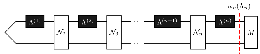
Figure 1: Illustration of a general adaptive protocol with $n$ black-box channels. The top row makes use of the given black-boxes while the bottom row depicts the memory system $R$.

For a set $\mathcal{S}_{n}$ corresponding to a hypothesis, we write $\omega_{n}(\mathcal{S}_{n})\coloneqq\Set{\omega_{n}(\mathcal{E}_{n})}{\mathcal{E}_{n}\in\mathcal{S}_{n}}$. Given an $\omega_{n}$, the problem then reduces to the composite state-discrimination problem $\omega_{n}(\mathcal{S}_{n})$ vs $\omega_{n}(\mathcal{T}_{n})$. Note that $\omega_{n}(\mathcal{S}_{n})\subset\mathcal{D}\left(R\otimes B\right)$, so this state discrimination problem will not be an instance of a many-copy discrimination problem as studied above, the $n$ just indicates how many channel black-boxes were used in obtaining the states in the set. We can again define the corresponding worst-case type II error exponent as

$$e_{A}(n,\varepsilon,\mathcal{S}_{n},\mathcal{T}_{n})\coloneqq\frac{1}{n}\sup_{\omega_{n}}D_{H}^{\varepsilon}(\omega_{n}(\mathcal{S}_{n})\|\omega_{n}(\mathcal{T}_{n}))=\frac{1}{n}\sup_{\omega_{n}}\sup_{\begin{subarray}{c}0\leq M\leq\IdentityMatrix\\ \alpha(M,\omega_{n}(\mathcal{S}_{n}))\leq\varepsilon\end{subarray}}\quantity[-\log\beta(M,\omega_{n}(\mathcal{T}_{n}))]$$ (57)

where the supremum over $\omega_{n}$ goes over all adaptive strategies, i.e. all initial states $\omega_{0}$ and all preparation maps $\mathcal{N}_{i}$, $i=2,...,n$.

4.2.1 An upper bound for adaptive strategies

We can prove the following upper bound on the Stein exponent for discriminating two composite channel hypotheses with adaptive strategies. This essentially captures the intuition that if the sets $\mathcal{S}_{n}$ and $\mathcal{T}_{n}$ are such that they include i.i.d. problem, then the error exponent has to be less than the worst-case i.i.d. error exponent.

Proposition 10.

Let $\bm{\mathcal{S}}=(\mathcal{S}_{n})_{n},\bm{\mathcal{T}}=(\mathcal{T}_{n})_{n}$ be two quantum composite channel hypotheses. Let $\mathcal{S}\coloneqq\mathcal{S}_{1}$ and $\mathcal{T}\coloneqq\mathcal{T}_{1}$. If the hypotheses are such that for all $n$

$$\mathcal{E}^{\otimes n} \in\mathcal{S}_{n}\quad\forall\,\mathcal{E}\in\mathcal{S}$$ (58)

$$\mathcal{F}^{\otimes n} \in\mathcal{T}_{n}\quad\forall\,\mathcal{F}\in\mathcal{T}$$ (59)

then the Stein exponent for distinguishing these two composite hypotheses by an adaptive strategy is upper bounded by

$$\lim_{\varepsilon\to 0}\lim_{n\to\infty}e_{A}(n,\varepsilon,\mathcal{S}_{n},\mathcal{T}_{n})\leq\min_{\begin{subarray}{c}\mathcal{E}\in\mathcal{S}\\ \mathcal{F}\in\mathcal{T}\end{subarray}}D_{A}(\mathcal{E}\|\mathcal{F})=\min_{\begin{subarray}{c}\mathcal{E}\in\mathcal{S}\\ \mathcal{F}\in\mathcal{T}\end{subarray}}D_{\mathrm{reg}}(\mathcal{E}\|\mathcal{F})\,.$$ (60)

Proof.

As mentioned above, let $\omega_{n}(\Lambda_{n})$ be the state at the end of the adaptive strategy with $n$ channel uses where the $n$ black-box channels are given by $\Lambda_{n}$. As specified above, given an $\omega_{n}$, the channel discrimination problem then reduces to the state-discrimination problem $\omega_{n}(\mathcal{S}_{n})$ vs. $\omega_{n}(\mathcal{T}_{n})$ with associated error exponent

$${1\over n}D_{H}^{\varepsilon}(\omega_{n}(\mathcal{S}_{n})\|\omega_{n}(\mathcal{T}_{n}))\,.$$ (61)

By 16 this is upper bounded as follows:

$${1\over n}D_{H}^{\varepsilon}(\omega_{n}(\mathcal{S}_{n})\|\omega_{n}(\mathcal{T}_{n})) \leq{1\over n}\inf_{\begin{subarray}{c}\rho_{n}\in\omega_{n}(\mathcal{S}_{n})\\ \sigma_{n}\in\omega_{n}(\mathcal{T}_{n})\end{subarray}}D_{H}^{\varepsilon}(\rho_{n}\|\sigma_{n})\leq{1\over n(1-\varepsilon)}\inf_{\begin{subarray}{c}\rho_{n}\in\omega_{n}(\mathcal{S}_{n})\\ \sigma_{n}\in\omega_{n}(\mathcal{T}_{n})\end{subarray}}D(\rho_{n}\|\sigma_{n})+o(1)$$ (62)

$$={1\over n(1-\varepsilon)}\inf_{\begin{subarray}{c}\mathcal{E}_{n}\in\mathcal{S}_{n}\\ \mathcal{F}_{n}\in\mathcal{T}_{n}\end{subarray}}D(\omega_{n}(\mathcal{E}_{n})\|\omega_{n}(\mathcal{F}_{n}))+o(1),$$ (63)

where the second inequality follows from 15. By using the sequential structure of the adaptive strategy, we find

$${1\over n}D(\omega_{n}(\mathcal{E}_{n})\|\omega_{n}(\mathcal{F}_{n}))\leq\sup_{k}\sup_{\rho,\sigma}\quantity[D(\mathcal{E}_{n}^{(k)}(\rho)\|\mathcal{F}_{n}^{(k)}(\sigma))-D(\rho\|\sigma)]$$ (64)

where $\mathcal{E}_{n}^{(k)}$ denote the $k^{th}$ channel in the tensor product of channels in $\mathcal{E}_{n}$. Since tensor products of the form $\mathcal{E}^{\otimes n}$ for $\mathcal{E}\in\mathcal{S}$ are included in $\mathcal{S}_{n}$ by assumption (and similarly for $\mathcal{T}_{n}$) this can be further upper bounded as (up to $o(1)$):

$${1\over n}D_{H}^{\varepsilon}(\omega_{n}(\mathcal{S}_{n})\|\omega_{n}(\mathcal{T}_{n}))\leq{1\over 1-\varepsilon}\inf_{\begin{subarray}{c}\mathcal{E}\in\mathcal{S}\\ \mathcal{F}\in\mathcal{T}\end{subarray}}\sup_{\rho,\sigma}\quantity[D(\mathcal{E}(\rho)\|\mathcal{F}(\sigma))-D(\rho\|\sigma)]={1\over 1-\varepsilon}\inf_{\begin{subarray}{c}\mathcal{E}\in\mathcal{S}\\ \mathcal{F}\in\mathcal{T}\end{subarray}}D_{A}(\mathcal{E}\|\mathcal{F})\,.$$ (65)

Finally, the $o(1)$ term disappears in the limit $n\to\infty$ and the factor $1\over{1-\varepsilon}$ goes to $1$ in the limit $\varepsilon\to 0$. Also, it is known [Fan+20] that $D_{A}(\mathcal{E}\|\mathcal{F})=D_{\mathrm{reg}}(\mathcal{E}\|\mathcal{F})$. The expression $\frac{1}{n}D(\mathcal{E}^{\otimes n}\|\mathcal{F}^{\otimes n})$ is monotonically increasing in $n$, and hence we can replace the limit $n\to\infty$ in the regularized divergence with a supremum over $n$. Hence the regularized divergence is lower semi-continuous (as a supremum of lower semi-continuous functions is lower semi-continuous), and hence the infimum is achieved. ∎

We will give a classical example in the next section where this upper bound is achieved and is strictly larger than the achievable exponent of parallel strategies. Hence this demonstrates an advantage of adaptive strategies for composite channel discrimination even if everything is classical.

Remark 11.

While the upcoming example demonstrates that this upper bound can sometimes be achieved, it cannot always be achieved. Hence, it is not a candidate for the optimal asymptotic exponent of adaptive strategies. This can be seen by taking all channels to be replacer channels. In this case the task of channel discrimination reduces to that of state discrimination, for which adaptive and parallel strategies are equivalent. In the composite i.i.d. setting (i.e. when $S_{n}=\Set{\rho^{\otimes n}}{\rho\in S}$ and $T_{n}=\Set{\sigma^{\otimes n}}{\sigma\in T}$) it has been shown that there exist sets $S$ and $T$ such that

$$\lim_{\varepsilon\to 0}\lim_{n\to\infty}D_{H}^{\varepsilon}(S_{n}\|T_{n})=\lim_{n\to\infty}{1\over n}\inf_{\begin{subarray}{c}\rho_{n}\in\mathcal{C}(S_{n})\\ \sigma_{n}\in\mathcal{C}(T_{n})\end{subarray}}D(\rho_{n}\|\sigma_{n})<\inf_{\begin{subarray}{c}\rho\in S\\ \sigma\in T\end{subarray}}D(\rho\|\sigma),$$ (66)

and different examples exist where $S$ and $T$ are either convex [BBH21, Section 4.2] or discrete [mosonyi_error_2021, Section IV.A].

4.2.2 A classical example of an adaptive advantage

In the following we give a fully classical example that demonstrates how adaptive strategies can be (also asymptotically) beneficial with composite hypotheses in the composite i.i.d. setting.

Example 12.

There exist classical composite channel hypotheses $\mathcal{S}=\{\mathcal{E}_{1},\mathcal{E}_{2}\}$ and $\mathcal{T}=\{\mathcal{F}_{1},\mathcal{F}_{2}\}$, such that the adaptive error exponent in the composite i.i.d. setting is strictly larger than the parallel one. Specifically, we show that

$$\lim_{\varepsilon\to 0}\lim_{n\to\infty}{1\over n}e_{A}(n,\varepsilon,\mathcal{S}_{n},\mathcal{T}_{n})=\min_{i,j\in\{1,2\}}D(\mathcal{E}_{i}\|\mathcal{F}_{j})=2\lim_{\varepsilon\to 0}\lim_{n\to\infty}{1\over n}e_{P}(n,\varepsilon,\mathcal{S}_{n},\mathcal{T}_{n})$$ (67)

where $\mathcal{S}_{n}=\Set{\mathcal{E}_{i}^{\otimes n}}{i=1,2}$, $\mathcal{T}_{n}=\Set{\mathcal{F}_{i}^{\otimes n}}{i=1,2}$.

When defining the channels, we will use quantum notation for convenience, but everything should be seen as classical, i.e. all states are diagonal in the computational basis.

The channels used in our example are then:

$$\mathcal{E}_{1}(\rho) =\tau\otimes\outerproduct{0}{0}$$ (68)

$$\mathcal{E}_{2}(\rho) =\tau\otimes\outerproduct{1}{1}$$ (69)

$$\mathcal{F}_{1}(\rho) =\frac{1}{2}\left[\tau+\braket{0}{\rho}{0}\outerproduct{0}{0}+\braket{1}{\rho}{1}\tau\right]\otimes\outerproduct{0}{0}$$ (70)

$$\mathcal{F}_{2}(\rho) =\frac{1}{2}\left[\tau+\braket{0}{\rho}{0}\tau+\braket{1}{\rho}{1}\outerproduct{0}{0}\right]\otimes\outerproduct{1}{1}$$ (71)

Where $\tau=\IdentityMatrix_{2}/2$ is the maximally mixed state. For notational simplicity, we denote $\mathcal{E}(0)\coloneqq\mathcal{E}(\outerproduct{0}{0})$, $\mathcal{E}(1)\coloneqq\mathcal{E}(\outerproduct{1}{1})$.

The adaptive strategy

The channels are constructed to allow for the following adaptive strategy: Given a black-box channel, we first use it with an arbitrary input state. Depending on the second output bit we will be able to determine with certainty the “index” of the channel, i.e. we will know that the channel is either $\mathcal{E}_{1}$ or $\mathcal{F}_{1}$ if the second bit is zero, or alternatively if the second bit is one we will know that the channel is either $\mathcal{E}_{2}$ or $\mathcal{F}_{2}$. It is easy to see that the optimal input state to discriminate $\mathcal{E}_{1}$ from $\mathcal{F}_{1}$ is $\outerproduct{0}{0}$, whereas the optimal input state to discriminate $\mathcal{E}_{2}$ from $\mathcal{F}_{2}$ is $\outerproduct{1}{1}$. Hence, in our adaptive strategy, for all subsequent channel uses, we input the value of the second bit we received out of the first channel use. This will lead to the following exponent:

$$\min_{i\in\{1,2\}}\,\max_{\rho\in\mathcal{D}\left(\mathcal{X}\right)}D(\mathcal{E}_{i}(\rho)\|\mathcal{F}_{i}(\rho))=D\big{(}\mathcal{E}_{1}(0)\|\mathcal{F}_{1}(0)\big{)}=D\big{(}\mathcal{E}_{2}(1)\|\mathcal{F}_{2}(1)\big{)}=\log_{2}(4/3)/2\,.$$ (72)

It is easy to see that this is also equal to

$$\min_{i,j\in\{1,2\}}\,\max_{\rho\in\mathcal{D}\left(\mathcal{X}\right)}D(\mathcal{E}_{i}(\rho)\|\mathcal{F}_{i}(\rho))$$ (73)

since this minimum is always achieved for $i=j$, as otherwise the second output bit allows for the two channels to be distinguished with certainty, which makes the relative entropy infinite. Since this is equal to the upper bound from 10 (for classical channels the regularized channel divergence collapses to the single-letter channel divergence), this is an asymptotically optimal adaptive strategy.

The best parallel strategy

By 14 below, the optimal parallel exponent is given by

$$\max_{\nu\in\mathcal{D}\left(\mathcal{X}^{\prime}\mathcal{X}\right)}\min_{\begin{subarray}{c}\mathcal{E}\in\mathcal{S}\\ \mathcal{F}\in T\end{subarray}}D(\mathcal{E}(\nu)\|\mathcal{F}(\nu))\,.$$ (74)

Similarly to the argument used in the proof of 14, by using the joint convexity of the relative entropy we find that for any state $\nu\in\mathcal{D}\left(\mathcal{X}^{\prime}\mathcal{X}\right)$ there exists a $p\in[0,1]$ such that for any $i,j$:

$$D(\mathcal{E}_{i}(\nu)\|\mathcal{F}_{j}(\nu))\leq pD(\mathcal{E}_{i}(0)\|\mathcal{F}_{j}(0))+(1-p)D(\mathcal{E}_{i}(1)\|F_{j}(1))\,,$$ (75)

and picking $\nu=p\outerproduct{00}{00}_{\mathcal{X}^{\prime}\mathcal{X}}+(1-p)\outerproduct{11}{11}_{\mathcal{X}^{\prime}\mathcal{X}}$ achieves the right-hand side. Hence, we can write:

$$\max_{\nu\in\mathcal{D}\left(\mathcal{X}^{\prime}\mathcal{X}\right)}\min_{\begin{subarray}{c}\mathcal{E}\in\mathcal{S}\\ \mathcal{F}\in T\end{subarray}}D(\mathcal{E}(\nu)\|\mathcal{F}(\nu))=\max_{0\leq p\leq 1}\,\min_{i,j\in\{1,2\}}\big{(}pD(\mathcal{E}_{i}(0)\|\mathcal{F}_{j}(0))+(1-p)D(\mathcal{E}_{i}(1)\|F_{j}(1))\big{)}\,.$$ (76)

Similarly to above, the minimum will be achieved at $i=j$, and it is easy to see by explicit computation that the optimum value of $p$ is $1/2$. Since $D(\mathcal{E}_{2}(0)\|\mathcal{F}_{2}(0))=D(\mathcal{E}_{1}(1)\|F_{1}(1))=0$ the parallel exponent is thus

$$\frac{1}{2}D\big{(}\mathcal{E}_{1}(0)\|\mathcal{F}_{1}(0)\big{)}$$ (77)

which is half the exponent we were able to achieve with the adaptive strategy. It is also easy to see that a way to achieves this parallel exponent is just to alternate the two input states $0$ and $1$.

4.2.3 Classical equality under convexity

Looking back at the previous example, one finds that the advantage of the adaptive strategy can be seen as coming from the fact that the order of the maximum over input states and minimum over channels (for example in (72)) matters: The parallel strategy has to find a good input state for all channels (this corresponds to taking the maximum over states outside), whereas the adaptive strategy can reduce the problem to a simple discrimination problem between just two channels and then tailor the input state to these two channels (this corresponds to taking the infimum over channels outside). Indeed, one also finds that an application of our exchange result 19 (or similar minimax theorems) is not permitted in this example, as the sets of channels $\mathcal{S}$ and $\mathcal{T}$ are not convex. We show subsequently that, in the classical case, convexity of these sets is indeed sufficient for there not to be an advantage of adaptive strategies.

Theorem 13.

Let $\bm{\mathcal{S}}=(\mathcal{S}_{n}\subset\mathrm{CPTP}(\mathcal{X}^{n}\to\mathcal{Y}^{n}))_{n},\bm{\mathcal{T}}=(\mathcal{T}_{n}\subset\mathrm{CPTP}(\mathcal{X}^{n}\to\mathcal{Y}^{n}))_{n}$ be two composite classical channel hypotheses (still satisfying the properties of 8). If $\mathcal{S}\coloneqq\mathcal{S}_{1}$ and $\mathcal{T}\coloneqq\mathcal{T}_{1}$ are convex, and additionally for all $n$

$$\mathcal{E}^{\otimes n} \in\mathcal{S}_{n}\quad\forall\mathcal{E}\in\mathcal{S}$$ (78)

$$\mathcal{F}^{\otimes n} \in\mathcal{T}_{n}\quad\forall\mathcal{F}\in\mathcal{T}$$ (79)

then the Stein exponent of distinguishing these two composite hypotheses is given by

$$\lim_{\varepsilon\to 0}\lim_{n\to\infty}e(n,\varepsilon,\mathcal{S}_{n},\mathcal{T}_{n})=\min_{\begin{subarray}{c}\mathcal{E}\in\mathcal{S}\\ \mathcal{F}\in\mathcal{T}\end{subarray}}\max_{\nu\in\mathcal{D}\left(\mathcal{X}\right)}D(\mathcal{E}(\nu)\|\mathcal{F}(\nu))$$ (80)

where this optimal exponent can be achieved with a parallel strategy.

Proof.

Achievability

Picking any classical input state $\nu\in\mathcal{D}\left(\mathcal{X}\right)$ and feeding identical copies of it into the $n$ classical channels, turns this problem into the classical composite hypothesis testing problem which is at most as hard as distinguishing the sets $P=\mathcal{S}[\nu]$, $Q=\mathcal{T}[\nu]$ in an adversarial setting (this follows from the properties of a composite channel hypothesis as specified in 8). Then, by Theorem 7, the exponent

$$\min_{p\in P,q\in Q}D(p\|q)$$ (81)

is achievable, and hence, by optimizing over $\nu$, also the exponent

$$\sup_{\nu\in\mathcal{D}\left(\mathcal{X}\right)}\min_{\begin{subarray}{c}p\in\mathcal{S}[\nu]\\ q\in\mathcal{T}[\nu]\end{subarray}}D(p\|q)=\sup_{\nu\in\mathcal{D}\left(\mathcal{X}\right)}\min_{\begin{subarray}{c}\mathcal{E}\in\mathcal{S}\\ \mathcal{F}\in\mathcal{T}\end{subarray}}D(\mathcal{E}(\nu)\|\mathcal{F}(\nu))$$ (82)

is achievable. Now, since $\mathcal{S}$ and $\mathcal{T}$ are convex, we can apply 19 and exchange the minimum and the supremum (where the supremum is also achieved, e.g. by 22).

Converse

From 10 we get:

$$\lim_{\varepsilon\to 0}\lim_{n\to\infty}e(n,\varepsilon,\mathcal{S}_{n},\mathcal{T}_{n})\leq\min_{\begin{subarray}{c}\mathcal{E}\in\mathcal{S}\\ \mathcal{F}\in\mathcal{T}\end{subarray}}D_{\mathrm{reg}}(\mathcal{E}\|\mathcal{F})\,.$$ (83)

If all channels $\mathcal{E}$ and $\mathcal{F}$ are classical, the regularization is not necessary [Hay09]. This can be easily seen follows: Since the relative entropy is jointly convex, the optimization over the input state is achieved at an extreme point of the convex set of input states, and classically all extreme points are product distributions, which makes the regularization collapse and also eliminates the need for any reference system. Hence

$$\lim_{\varepsilon\to 0}\lim_{n\to\infty}e(n,\varepsilon,\mathcal{S}_{n},\mathcal{T}_{n})\leq\min_{\begin{subarray}{c}\mathcal{E}\in\mathcal{S}\\ \mathcal{F}\in\mathcal{T}\end{subarray}}\max_{\nu\in\mathcal{D}\left(\mathcal{X}\right)}D(\mathcal{E}(\nu)\|\mathcal{F}(\nu))$$ (84)

which is what we wanted to prove.

∎

4.3 Classical parallel exponent for finite sets in the composite i.i.d. setting

Theorem 13 leaves open the question what we can say about adaptive and parallel exponents with classical channels if the sets $\mathcal{S}$ and $\mathcal{T}$ are non-convex. 12 shows that these two exponents have to be different in general, however we would still like to find entropic expressions for them. The following proposition establishes a single-letter formula for the parallel exponent in the composite i.i.d. case when the two sets $\mathcal{S}$ and $\mathcal{T}$ are finite.

Proposition 14.

Let $\mathcal{S}$, $\mathcal{T}\subset\mathrm{CPTP}(\mathcal{X}\to\mathcal{Y})$ be two finite sets of classical channels. In the composite i.i.d setting, i.e. with

$$\mathcal{S}_{n} \coloneqq\Set{\mathcal{E}^{\otimes n}}{\mathcal{E}\in\mathcal{S}}$$ (85)

$$\mathcal{T}_{n} \coloneqq\Set{\mathcal{F}^{\otimes n}}{\mathcal{F}\in\mathcal{T}}$$ (86)

the Stein exponent of distinguishing these two hypotheses with a parallel strategy is given by

$$\lim_{\varepsilon\to 0}\lim_{n\to\infty}e_{P}(n,\varepsilon,\mathcal{S}_{n},\mathcal{T}_{n})=\max_{\nu\in\mathcal{D}\left(\mathcal{X}^{\prime}\mathcal{X}\right)}\min_{\begin{subarray}{c}\mathcal{E}\in\mathcal{S}\\ \mathcal{F}\in\mathcal{T}\end{subarray}}D(\mathcal{E}(\nu)\|\mathcal{F}(\nu))\,,$$ (87)

where $\mathcal{X}^{\prime}$ is another classical system with the size of $\mathcal{X}$.

Proof.

Achievability

Again, picking any classical input state $\nu\in\mathcal{D}\left(\mathcal{X}^{\prime}\mathcal{X}\right)$ and feeding identical copies of it into the $n$ classical channels, turns this problem into the classical composite i.i.d. hypothesis testing problem of distinguishing the sets $P=\mathcal{S}[\nu]$, $Q=\mathcal{T}[\nu]$. Since they are both finite, we can apply [mosonyi_error_2021, Theorem III.2], which states that the optimal exponent of this composite state discrimination problem is given by

$$\min_{p\in P,q\in Q}D(P\|Q)=\min_{\begin{subarray}{c}\mathcal{E}\in\mathcal{S}\\ \mathcal{F}\in\mathcal{T}\end{subarray}}D(\mathcal{E}(\nu)\|\mathcal{F}(\nu))\,.$$ (88)

Taking the supremum over all input states $\nu$ yields the desired achievability result, and the supremum is achieved by an argument similar to 22, as the minimum over a finite number of elements does not affect any of the required continuity properties.

Converse

It follows immediately from the definition (31), 16 and 15 that

$$\frac{1}{n}D_{H}^{\varepsilon}(\mathcal{S}_{n}\|\mathcal{T}_{n}) =\frac{1}{n}\sup_{\nu_{n}\in\mathcal{D}\left(R\mathcal{X}^{n}\right)}D_{H}^{\varepsilon}(\mathcal{S}_{n}[\nu_{n}]\|\mathcal{T}_{n}[\nu_{n}])$$ (89)

$$\leq{1\over n(1-\varepsilon)}\sup_{\nu_{n}\in\mathcal{D}\left(R\mathcal{X}^{n}\right)}\inf_{\begin{subarray}{c}\mathcal{E}\in\mathcal{S}\\ \mathcal{F}\in\mathcal{T}\end{subarray}}D(\mathcal{E}^{\otimes n}(\nu_{n})\|\mathcal{F}^{\otimes n}(\nu_{n}))+o(1)\,.$$ (90)

where strictly speaking $R$ could be a quantum system, and hence $\nu_{n}$ a quantum-classical state of the form

$$\nu_{n}=\sum_{i=1}^{d^{n}}p_{i}\rho_{R}^{(i)}\otimes\outerproduct{i}{i}_{\mathcal{X}^{n}}$$ (91)

where $\{p_{i}\}_{i=1}^{d^{n}}$ is a probability distribution and the $\rho_{R}^{(i)}$ are density matrices on $R$.

By using the joint convexity of relative entropy and additivity under tensor products, it is easy to see though that for any such state $\nu_{n}$ there exists a probability distribution $\{q_{i}\}_{i=1}^{d}$ such that for all channels $\mathcal{E}$ and $\mathcal{F}$:

$${1\over n}D(\mathcal{E}^{\otimes n}(\nu_{n})\|\mathcal{F}^{\otimes n}(\nu_{n}))\leq\sum_{i=1}^{d}q_{i}D(\mathcal{E}(\outerproduct{i}{i})\|\mathcal{F}(\outerproduct{i}{i}))=D(\mathcal{E}(\nu)\|\mathcal{F}(\nu))\,.$$ (92)

where $\nu=\sum_{i}q_{i}\outerproduct{i}{i}_{\mathcal{X}^{\prime}}\otimes\outerproduct{i}{i}_{\mathcal{X}}$. Hence, we can upper bound the last part of (90) with the single-letter expression

$${1\over(1-\varepsilon)}\sup_{\nu\in\mathcal{D}\left(\mathcal{X}^{\prime}\mathcal{X}\right)}\min_{\begin{subarray}{c}\mathcal{E}\in\mathcal{S}\\ \mathcal{F}\in\mathcal{T}\end{subarray}}D(\mathcal{E}(\nu)\|\mathcal{F}(\nu))+o(1)$$ (93)

and the statement follows in the limit $n\to\infty$, $\varepsilon\to 0$.

∎

5 Open Problems

We have been able to provide new insight into the relation between adaptive and parallel channel discrimination strategies, by studying such strategies for composite channel hypotheses and demonstrating that there is a gap in the asymptotic setting. However, there are still many open questions regarding composite channel discrimination, as can be seen by the number of cells in Table 1 for which we cannot give a definitive answer. Here, we want to briefly describe some of these problems and elaborate on possible solutions.

First of all, for classical composite hypotheses which are non-convex, we currently do not have an entropic expression for the optimal achievable rate of adaptive strategies, so far we have not even been able to prove that the worst-case i.i.d. upper bound cannot always be achieved. Intuitively though, we consider it to be unlikely that this bound is always achieved, and we are also not particularly hopeful that there will be a simple entropic formula for the adaptive exponent. This comes from imagining generalizations of 12: In our example, determining the index of the channel within the two sets was possible perfectly after only one use, and hence one was able to use the optimal input state for all subsequent channel uses. One could, however, think about examples where determining this index is not perfectly possible, and hence one is expected to have to pay a certain (asymptotically non-vanishing) number of channel uses to distinguish the individual elements of the sets and then prepare the best input state, which should make the upper bound of 10 not achievable in this case. This procedure of determining which channels in the set we seem to be provided with also becomes significantly more complex once one stops having the symmetry between the sets $\mathcal{S}$ and $\mathcal{T}$ which we have in 12, and in the general case it is not obvious at all how one could capture in a simple entropic expression the intricacies of gaining knowledge about which elements in this set one might be given.

Additionally, we would like to see if there is an advantage for adaptive strategies in the quantum composite i.i.d. case when the sets of channels $\mathcal{S}_{1}$ and $\mathcal{T}_{1}$ are convex (recall that we showed that this is not possible classically). Given that the regularization is necessary in general in the quantum case, and the sets $\mathcal{S}_{n}$ and $\mathcal{T}_{n}$ will not be convex even if $\mathcal{S}_{1}$ and $\mathcal{T}_{1}$ are, we consider it not unlikely that there will again be an asymptotic gap between adaptive and parallel strategies.

Finally, we have only studied asymmetric error exponents in this work, even though it would of course also be very interesting to look at similar problems for symmetric error exponents and potentially also Hoeffding exponents.

helstrom_quantum_1976helstrom_quantum_1969 mosonyi_error_2021mosonyi_error_2022

Appendix A Technical Lemmas

Lemma 15 is a well-known consequence of the data-processing inequality of the relative entropy and has been widely used in converse proofs in information theory. A statement and proof using our notation can be found in [WR12], although the essence of the statement can already be found much earlier, for example in [HP91, Theorem 2.2] and also [Hay06, (3.30)].

Lemma 15 (Upper bound on $D_{H}^{\varepsilon}$).

Let $\rho,\sigma\in\mathcal{D}\left(\mathcal{H}\right)$ be quantum states. Then for all $\varepsilon\in[0,1)$

$$D_{H}^{\varepsilon}(\rho\|\sigma)\leq\frac{1}{1-\varepsilon}\big{(}D(\rho\|\sigma)+h(\varepsilon)\big{)},$$ (94)

where $h(\varepsilon)$ is the binary entropy function.

Lemma 16.

For any two sets of states $S$ and $T$, and any $\varepsilon\in[0,1]$,

$$D_{H}^{\varepsilon}(S\|T)\leq\inf_{\begin{subarray}{c}\rho\in S\\ \sigma\in T\end{subarray}}D_{H}^{\varepsilon}(\rho\|\sigma),$$ (95)

where the intuition is that the left-hand side corresponds to choosing one measurement for all pairings of $\rho$ and $\sigma$, and the right-hand side allows for a different measurement for each pairing.

Proof.

One finds that

$$2^{-D_{H}^{\varepsilon}(S\|T)} =\inf_{\begin{subarray}{c}0\leq M\leq\IdentityMatrix\\ \sup_{\rho\in S}\Tr(\bar{M}\rho)\leq\varepsilon\end{subarray}}\sup_{\sigma\in T}\Tr(M\sigma)\geq\sup_{\rho\in S}\inf_{\begin{subarray}{c}0\leq M\leq\IdentityMatrix\\ \Tr(\bar{M}\rho)\leq\varepsilon\end{subarray}}\sup_{\sigma\in T}\Tr(M\sigma)$$ (96)

$$\geq\sup_{\rho\in S}\sup_{\sigma\in T}\inf_{\begin{subarray}{c}0\leq M\leq\IdentityMatrix\\ \Tr(\bar{M}\rho)\leq\varepsilon\end{subarray}}\Tr(M\sigma)=\sup_{\begin{subarray}{c}\rho\in S\\ \sigma\in T\end{subarray}}2^{-D^{\varepsilon}_{H}(\rho\|\sigma)}$$ (97)

where we used the notation $\bar{M}=\IdentityMatrix-M$, and the first inequality can be seen as follows: For any $\rho\in S$, if an $M$ is chosen such that $\sup_{\rho^{\prime}\in S}\Tr(\bar{M}\rho^{\prime})\leq\varepsilon$, then obviously also $\Tr(\bar{M}\rho)\leq\varepsilon$ and hence the infimum on the right-hand is over a set of $M$ which can only be larger, and hence the expression can only be smaller. The second inequality is just a very basic property of infima and suprema, and the desired statement then follows by taking negative logarithms. ∎

The following is a standard argument used to show that the size of reference systems can be restricted. We prove it again here for completeness in a setting that also includes infima over channels.

Lemma 17.

Let $\mathbf{D}$ be a quantum divergence satisfying the data-processing inequality, and let $\mathcal{S},\mathcal{T}\subset\mathrm{CPTP}(A\to B)$ be two arbitrary sets of channels. Then,

$$\sup_{\begin{subarray}{c}\nu\in\mathcal{D}\left(R\otimes A\right)\\ R\text{ arbitrary}\end{subarray}}\inf_{\begin{subarray}{c}\mathcal{E}\in\mathcal{S}\\ \mathcal{F}\in\mathcal{T}\end{subarray}}\mathbf{D}(\mathcal{E}(\nu)\|\mathcal{F}(\nu))=\sup_{\begin{subarray}{c}\nu\in\mathcal{D}\left(R\otimes A\right)\\ R\cong A\end{subarray}}\inf_{\begin{subarray}{c}\mathcal{E}\in\mathcal{S}\\ \mathcal{F}\in\mathcal{T}\end{subarray}}\mathbf{D}(\mathcal{E}(\nu)\|\mathcal{F}(\nu)),$$ (98)

i.e. the size of the system $R$ can be restricted to be isomorphic to $A$.

Proof.

Let $R$ be an arbitrary reference system, and consider a state $\nu_{RA}\in\mathcal{D}\left(R\otimes A\right)$. Let $\nu$ have a purification $\nu_{PRA}$. Furthermore, take the state $\nu_{A}=\Tr_{R}\nu_{AR}$ and its canonical purification $\nu_{SA}$, where $S\cong A$ (it is well known that such a canonical purification always exists). Then, as also $\nu_{PRA}$ is a purification of $\nu_{A}$, $\nu_{PRA}$ and $\nu_{SA}$ are related by an isometry $V:PR\to S$. As the channels $\mathcal{E}$ and $\mathcal{F}$ act as identity on these systems the isometry commutes with them, and as any divergence satisfying the data-processing property is invariant under isometries (see e.g. [KW20])

$$D(\mathcal{E}(\nu_{RA})\|\mathcal{F}(\nu_{RA}))\leq D(\mathcal{E}(\nu_{PRA})\|\mathcal{F}(\nu_{PRA}))=D(\mathcal{E}(\nu_{SA})\|\mathcal{F}(\nu_{SA})))$$ (99)

and hence the supremum can be restricted to reference systems isomorphic to $A$. Note that the set $\mathbf{D}(S\otimes A)=\mathbf{D}(A\otimes A)$ is compact. ∎

Lemma 18 (Generalized minimax theorem [FR06, Theorem 5.2]).

Let $X$ be a compact and convex subset of a Hausdorff topological vector space and let $Y$ be a convex subset of a linear space. Let $f:X\times Y\to\mathbb{R}\cup\{\infty\}$ be lower semi-continuous on $X$ for fixed $y\in Y$, convex in x and concave in y. Then

$$\sup_{y\in Y}\inf_{x\in X}f(x,y)=\inf_{y\in Y}\sup_{x\in X}f(x,y)\,.$$ (100)

We say that a divergence $\mathbf{D}$ satisfies the direct-sum property, if

$$\mathbf{D}\left(\bigoplus_{i=1}^{n}p_{i}\rho_{i}\;\middle\|\;\bigoplus_{i=1}^{n}p_{i}\sigma_{i}\right)=\sum_{i=1}^{n}p_{i}\mathbf{D}(\rho_{i}\|\sigma_{i})\,.$$ (101)

whenever $\rho_{i},\sigma_{i}\in\mathcal{H}_{i}$ are two sets of density matrices and $\{p_{i}\}_{i=1}^{n}$ is a probability distribution.

Proposition 19.

Let $\mathcal{S},\mathcal{T}\subset\mathrm{CPTP}(A\to B)$ be two closed, convex sets of channels. Let $\mathbf{D}$ be a quantum divergence that satisfies the data-processing inequality, is (jointly) lower semi-continuous, and also satisfies the direct-sum property. Then

$$\inf_{\begin{subarray}{c}\mathcal{E}\in\mathcal{S}\\ \mathcal{F}\in\mathcal{T}\end{subarray}}\sup_{\nu\in\mathcal{D}\left(R\otimes A\right)}\mathbf{D}(\mathcal{E}(\nu)\|\mathcal{F}(\nu))=\sup_{\nu\in\mathcal{D}\left(R\otimes A\right)}\inf_{\begin{subarray}{c}\mathcal{E}\in\mathcal{S}\\ \mathcal{F}\in\mathcal{T}\end{subarray}}\mathbf{D}(\mathcal{E}(\nu)\|\mathcal{F}(\nu)).$$ (102)

Proof.

This proof is inspired by the proof of the similar minimax result [Bra+20, Lemma 13]. The $\geq$ direction follows immediately from very basic properties of $\inf$ and $\sup$. For the $\leq$ direction, let $\mu$ be a discrete measure on the set of density matrices $\mathcal{D}\left(RA\right)$, and consider the function:

$$f((\mathcal{E},\mathcal{F}),\mu)\coloneqq\underset{\nu\sim\mu}{\mathbb{E}}\mathbf{D}(\mathcal{E}(\nu)\|\mathcal{F}(\nu))\,.$$ (103)

where we write $\underset{\nu\sim\mu}{\mathbb{E}}$ for the expectation value with respect to the measure $\mu$ (this is the same as integrating $\nu$ with respect to the measure $\mu$). It is easy to see that a divergence that satisfies the data-processing inequality and the direct-sum property is jointly convex (see e.g. [KW20]). Hence the function $f$ is convex in its first argument, and it is clearly also linear (and hence concave) in the second argument. Note also that the set of channels $\mathrm{CPTP}(A\to B)$ is bounded (for example in diamond norm) and hence compact, and so are the closed subsets $\mathcal{S}$ and $\mathcal{T}$. Then, by 18 we have

$$\inf_{\begin{subarray}{c}\mathcal{E}\in\mathcal{S}\\ \mathcal{F}\in\mathcal{T}\end{subarray}}\sup_{\mu}\underset{\nu\sim\mu}{\mathbb{E}}\mathbf{D}(\mathcal{E}(\nu)\|\mathcal{F}(\nu))=\sup_{\mu}\inf_{\begin{subarray}{c}\mathcal{E}\in\mathcal{S}\\ \mathcal{F}\in\mathcal{T}\end{subarray}}\underset{\nu\sim\mu}{\mathbb{E}}\mathbf{D}(\mathcal{E}(\nu)\|\mathcal{F}(\nu)).$$ (104)

We can lower bound the left-hand side by restricting the supremum to singular (i.e. Dirac) measures, which recovers the left-hand side of (102). For the right-hand side, note that by Caratheodory’s theorem we can write the expectation value as a convex combination with a finite number of terms. For a given $\mu$ we will write

$$\underset{\nu\sim\mu}{\mathbb{E}}\mathbf{D}(\mathcal{E}(\nu)\|\mathcal{F}(\nu))=\sum_{x}p_{x}\mathbf{D}(\mathcal{E}(\nu_{x})\|\mathcal{F}(\nu_{x})).$$ (105)

Now define the new state

$$\tilde{\nu}_{XRA}\coloneqq\sum_{x}p_{x}\outerproduct{x}{x}\otimes\nu_{x}.$$ (106)

By the direct-sum property of $\mathbf{D}$ (note that $\mathcal{E}$ and $\mathcal{F}$ act with an identity on the new system $X$)

$$\mathbf{D}(\mathcal{E}(\tilde{\nu})\|\mathcal{F}(\tilde{\nu}))=\sum_{x}p_{x}\mathbf{D}(\mathcal{E}(\nu_{x})\|\mathcal{F}(\nu_{x}))$$ (107)

And so the supremum over measures can be replaced by a supremum over states $\nu_{XRA}$. Finally, by 17 the supremum can further be restricted to states $\nu_{RA}$ where $R\cong A$. ∎

It is well-known (see e.g. [KW20]) that the properties of $\mathbf{D}$ required in 19 are satisfied for the Umegaki relative entropy. They are also satisfied for the measured relative entropy:

Lemma 20.

The measured relative entropy $D_{M}$ satisfies the data-processing inequality, is lower semi-continuous, and satisfies the direct-sum property.

Proof.

For the data-processing inequality it is easy to see that concatenating a POVM $\mathcal{M}$ (treated as a classical-quantum channel as explained in the mathematical preliminaries) and an arbitrary quantum channel $\mathcal{E}$ as $\mathcal{M}\circ\mathcal{E}$ yields another POVM, and hence $D_{M}$ satisfies the data-processing inequality as the supremum over all POVMs of the form $\mathcal{M}\circ\mathcal{E}$ can only be smaller than the supremum over all POVMs. $D_{M}$ is also lower semi-continuous as a supremum of lower semi-continuous functions is lower semi-continuous, and $D$ is lower semi-continuous. For the direct-sum property, let $\mathcal{H}=\bigoplus_{i=1}^{n}\mathcal{H}_{i}$, and $\rho_{i}$, $\sigma_{i}\in\mathcal{D}\left(\mathcal{H}_{i}\right)$ be two sets of density matrices, $\mathcal{M}_{i}$ be a set of POVMs each on $\mathcal{H}_{i}$ and $\{p_{i}\}_{i}$ be a probability distribution, where all indices are in the range $i=1,...n$. Define $\rho=\bigoplus_{i=1}^{n}p_{i}\rho_{i}$, $\sigma=\bigoplus_{i=1}^{n}p_{i}\sigma_{i}$ and $\bar{\mathcal{M}}\coloneqq\bigoplus_{i=1}^{n}\mathcal{M}_{i}$. It is easy to see that

$$\bar{\mathcal{M}}\quantity(\bigoplus_{i=1}^{n}p_{i}\rho_{i})=\bigoplus_{i=1}^{n}p_{i}\mathcal{M}_{i}(\rho_{i})$$ (108)

and hence

$$D_{M}\left(\bigoplus_{i=1}^{n}p_{i}\rho_{i}\;\middle\|\;\bigoplus_{i=1}^{n}p_{i}\sigma_{i}\right) \geq D\left(\bar{M}\quantity(\bigoplus_{i=1}^{n}p_{i}\rho_{i})\;\middle\|\;\bar{M}\quantity(\bigoplus_{i=1}^{n}p_{i}\sigma_{i})\right)$$ (109)

$$=D\left(\bigoplus_{i=1}^{n}p_{i}\mathcal{M}_{i}(\rho_{i})\;\middle\|\;\bigoplus_{i=1}^{n}p_{i}\mathcal{M}_{i}(\sigma_{i})\right)$$ (110)

$$=\sum_{i=1}^{n}p_{i}D(\mathcal{M}_{i}(\rho_{i})\|\mathcal{M}_{i}(\sigma_{i})),$$ (111)

which leads to the $\geq$ direction in the direct-sum property after optimizing over the $\mathcal{M}_{i}$. For the reverse direction, let $\mathcal{M}$ be an arbitrary POVM on $\mathcal{H}$. Then

$$D(\mathcal{M}(\rho)\|\mathcal{M}(\sigma))=D\left(\sum_{i}p_{i}\mathcal{M}(\rho_{i})\;\middle\|\;\sum_{i}p_{i}\mathcal{M}(\sigma_{i})\right)\leq\sum_{i}p_{i}D(\mathcal{M}(\rho_{i})\|\mathcal{M}(\sigma_{i}))\leq\sum_{i}p_{i}D_{M}(\rho_{i}\|\sigma_{i}),$$ (112)

where we used the joint convexity of the relative entropy. The claim follows by optimizing over all $\mathcal{M}$. ∎

Lemma 21.

Let $\mathcal{E},\mathcal{F}\in\mathrm{CPTP}(A\to B)$ be such that $D_{\max}(\mathcal{E}\|\mathcal{F})<\infty$, and let $R$ be an arbitrary auxiliary system. Then the function

$$(\mathcal{M},\nu)\mapsto D(\mathcal{M}\circ\mathcal{E}(\nu)\|\mathcal{M}\circ\mathcal{F}(\nu))$$ (113)

is continuous on $\mathrm{CPTP}(B\to C)\times\mathcal{D}\left(R\otimes A\right)$.

Proof.

It is easy to see that for $0<\alpha<1$ the Petz-Rényi divergence [Pet86]

$$D_{\alpha}(\rho\|\sigma)\coloneqq\frac{1}{\alpha-1}\log\Tr(\rho^{\alpha}\sigma^{1-\alpha})$$ (114)

is jointly continuous in $\rho$ and $\sigma$. Using the continuity bound from [Ber+22, Lemma 9], we find

$$|D_{\alpha}(\rho\|\sigma)-D(\rho\|\sigma)|\leq(1-\alpha)\log^{2}\quantity(2^{D_{\max}(\rho\|\sigma)}+2)\,.$$ (115)

As $D_{\max}(\mathcal{M}\circ\mathcal{E}(\nu)\|\mathcal{M}\circ\mathcal{F}(\nu))\leq D_{\max}(\mathcal{E}\|\mathcal{F})$ which is independent of $\mathcal{M}$ and $\nu$, we get that $D_{\alpha}(\mathcal{M}\circ\mathcal{E}(\nu)\|\mathcal{M}\circ\mathcal{F}(\nu))$ converges to $D(\mathcal{M}\circ\mathcal{E}(\nu)\|\mathcal{M}\circ\mathcal{F}(\nu))$ uniformly in $\nu$ and $\mathcal{M}$ as $\alpha\uparrow 1$. Hence, also the limiting function $(\mathcal{M},\nu)\mapsto D(\mathcal{M}\circ\mathcal{E}(\nu)\|\mathcal{M}\circ\mathcal{F}(\nu))$ is continuous. ∎

Lemma 22.

Let $\mathcal{E},\mathcal{F}\in\mathrm{CPTP}(A\to B)$, and $R$ be an arbitrary auxiliary system. Then, if $\mathbf{D}$ is either $D$ or $D_{M}$:

$$\sup_{\nu\in\mathcal{D}\left(R\otimes A\right)}\mathbf{D}(\mathcal{E}(\nu)\|\mathcal{F}(\nu))=\max_{\begin{subarray}{c}\nu\in\mathcal{D}\left(R\otimes A\right)\\ R\cong A\end{subarray}}\mathbf{D}(\mathcal{E}(\nu)\|\mathcal{F}(\nu))$$ (116)

i.e. the supremum is achieved and $R$ can be chosen isomorphic to $A$.

Proof.

The restriction to $R$ isomorphic to $A$ follows from 17. What remains to show is that the supremum is achieved. Consider first the case where $D_{\max}(\mathcal{E}\|\mathcal{F})=\infty$. As shown in [Wil+20], $D_{\max}(\mathcal{E}\|\mathcal{F})=D_{\max}(\mathcal{E}(\Omega)\|\mathcal{F}(\Omega))$ where $\Omega=\Omega_{RA}$ is a maximally entangled state. It is well known that (in finite dimensions) $D_{\max}(\rho\|\sigma)=\infty\Rightarrow D(\rho\|\sigma)=\infty$ for all states $\rho$, $\sigma$, and hence if $\mathbf{D}=D$ the value of infinity is achieved in this case. It is also not hard to see that if $D(\rho\|\sigma)=\infty$ also $D_{M}(\rho\|\sigma)=\infty$ (in this case $\sigma$ will have a smaller support than $\rho$, so a POVM built from the projection onto the support of $\sigma$ will achieve infinity). Hence in this case also with $\mathbf{D}=D_{M}$ the supremum is achieved. So assume $D_{\max}(\mathcal{E}\|\mathcal{F})<\infty$. If $\mathbf{D}=D$, then by 21, the function is continuous in $\nu$ and hence, since the set of density matrices optimized over is compact, the optimum value is achieved. If $\mathbf{D}=D_{M}$ we have the expression

$$\sup_{\nu\in\mathcal{D}\left(R\otimes A\right)}D_{M}(\mathcal{E}(\nu)\|\mathcal{F}(\nu))=\sup_{\nu\in\mathcal{D}\left(R\otimes A\right)}\sup_{\mathcal{M}\text{ POVM}}D(\mathcal{M}\circ\mathcal{E}(\nu)\|\mathcal{M}\circ\mathcal{F}(\nu))$$ (117)

Again, by 21 the expression optimized over is continuous in $\nu$ and $\mathcal{M}$. Also, by [BFT17] the optimization over $\mathcal{M}$ in the measured relative entropy can be restricted to von Neumann measurements (i.e. projective rank-1 measurements), and the set of these measurements is compact (as such a measurement is uniquely specified by a unitary matrix). Hence, also here the optimum value is achieved. ∎

We say that a state $\rho_{n}\in\mathcal{D}\left(\mathcal{H}^{\otimes n}\right)$ is permutation invariant, if for any permutation of $n$ systems $\pi\in S(n)$ and associated unitary operator $\Pi$ it holds that $\Pi\rho_{n}\Pi=\rho_{n}$. We say that a channel $\mathcal{E}_{n}\in\mathrm{CPTP}(A^{n}\to B^{n})$ is permutation covariant if $\mathcal{E}_{n}(\Pi_{A}\rho_{n}\Pi_{A})=\Pi_{B}\mathcal{E}_{n}(\rho_{n})\Pi_{B}$ for all input states $\rho_{n}\in\mathcal{D}\left(\mathcal{H}^{\otimes n}\right)$ and all permutations $\pi\in S(n)$ and associated canonical representations $\Pi_{A}$ on $A^{n}$ and $\Pi_{B}$ on $B^{n}$. We say a set of channels $\mathcal{S}_{n}\subset\mathrm{CPTP}(A^{n}\to B^{n})$ is closed under permutations, if for any $\mathcal{E}_{n}\in\mathcal{S}_{n}$ and any permutation $\pi\in S(n)$, with associated representations $\Pi_{A}$ on $A^{n}$ and $\Pi_{B}$ on $B^{n}$, also the channel with permuted input and output systems $\rho\mapsto\Pi_{B}\mathcal{E}_{n}(\Pi_{A}\rho\Pi_{A})\Pi_{B}$ is an element of $\mathcal{S}_{n}$.

Lemma 23.

Let $\mathcal{S}_{n}$, $\mathcal{T}_{n}\subset\mathrm{CPTP}(A^{n}\to B^{n})$ be closed convex and also closed under permutations, and let $\mathbf{D}$ be lower semi-continuous and satisfy the data-processing inequality. Then,

$$\inf_{\begin{subarray}{c}\mathcal{E}_{n}\in S_{n}\\ \mathcal{F}_{n}\in T_{n}\end{subarray}}\sup_{\begin{subarray}{c}\nu\in\mathcal{D}\left(R\otimes A^{\otimes n}\right)\\ R\text{ arbitrary}\end{subarray}}\mathbf{D}(\mathcal{E}_{n}(\nu)\|\mathcal{F}_{n}(\nu))=\min_{\begin{subarray}{c}\mathcal{E}_{n}\in S_{n}\\ \mathcal{F}_{n}\in T_{n}\\ \mathcal{E}_{n},\mathcal{F}_{n}\text{ perm. covariant.}\end{subarray}}\sup_{\begin{subarray}{c}\nu\in\mathcal{D}\left(R\otimes A^{\otimes n}\right)\\ R\text{ arbitrary}\end{subarray}}\mathbf{D}(\mathcal{E}_{n}(\nu)\|\mathcal{F}_{n}(\nu))$$ (118)

i.e. the infimum is achieved for permutation covariant elements of $\mathcal{S}_{n}$ and $\mathcal{T}_{n}$.

Proof.

First, the infimum is achieved since the infimum of a lower semi-continuous function over a compact set is achieved, and the supremum of a lower semi-continuous function is lower semi-continuous. Let $\mathcal{E}_{n}\in S_{n}$ and $\mathcal{F}_{n}\in T_{n}$ be two channels, and consider the permuted versions:

$$\bar{\mathcal{E}}_{n}(\rho) \coloneqq\frac{1}{n!}\sum_{\Pi\in S(n)}\Pi_{B}\mathcal{E}_{n}(\Pi_{A}\rho\Pi_{A})\Pi_{B}$$ (119)

$$\bar{\mathcal{F}}_{n}(\rho) \coloneqq\frac{1}{n!}\sum_{\Pi\in S(n)}\Pi_{B}\mathcal{F}_{n}(\Pi_{A}\rho\Pi_{A})\Pi_{B}$$ (120)

This can be seen as a permutation super-channel applied to $\mathcal{E}_{n}$ and $\mathcal{F}_{n}$, and it is known that any channel divergence can only decrease under such super-channels (see e.g. [Gou19]), however, we will still show this explicitly again here for the reader’s convenience:

Define the channel $\mathcal{A}:A^{n}\to A^{n}\otimes R^{\prime}$

$$\mathcal{A}(\rho)\coloneqq\frac{1}{n!}\sum_{\Pi\in S(n)}(\Pi_{A}\rho\Pi_{A})\otimes\outerproduct{\Pi}{\Pi}_{R^{\prime}}$$ (121)

where $R^{\prime}$ is some additional classical register storing the permutation $\Pi$. Defining $\mathcal{B}:B^{n}\otimes R^{\prime}\to B^{n}$:

$$\mathcal{B}(\rho)\coloneqq\sum_{\Pi\in S(n)}\Pi_{B}\bra{\Pi}_{R^{\prime}}\rho\ket{\Pi}_{R^{\prime}}\Pi_{B}$$ (122)

we find that

$$\bar{\mathcal{E}}_{n}=\mathcal{B}\circ(\mathcal{E}_{n}\otimes\textrm{id}_{R^{\prime}})\circ\mathcal{A}$$ (123)

$$\bar{\mathcal{F}}_{n}=\mathcal{B}\circ(\mathcal{F}_{n}\otimes\textrm{id}_{R^{\prime}})\circ\mathcal{A}\,.$$ (124)

Hence

$$\sup_{\begin{subarray}{c}\nu\in\mathcal{D}\left(R\otimes A^{\otimes n}\right)\\ R\text{ arbitrary}\end{subarray}}\mathbf{D}(\bar{\mathcal{E}}_{n}(\nu)\|\bar{\mathcal{F}}_{n}(\nu))\leq\sup_{\begin{subarray}{c}\nu\in\mathcal{D}\left(R\otimes A^{\otimes n}\right)\\ R\text{ arbitrary}\end{subarray}}\mathbf{D}(\mathcal{E}_{n}(\mathcal{A}(\nu))\|\mathcal{F}_{n}(\mathcal{A}(\nu)))\leq\sup_{\begin{subarray}{c}\nu\in\mathcal{D}\left(R\otimes A^{\otimes n}\right)\\ R\text{ arbitrary}\end{subarray}}\mathbf{D}(\mathcal{E}_{n}(\nu)\|\mathcal{F}_{n}(\nu))$$ (125)

where the first inequality is the normal data-processing inequality (we omitted the $\textrm{id}_{R^{\prime}}$), and the second inequality uses that all the states $\mathcal{A}(\nu)$ are itself included in the supremum. As it is easy to see that the channels $\bar{\mathcal{E}}_{n}$ and $\bar{\mathcal{F}}_{n}$ are permutation covariant and are also included in $\mathcal{S}_{n}$ and $\mathcal{T}_{n}$ (as they were assumed to be closed under complete permutations), the minimum will be achieved for permutation covariant channels. ∎

Lemma 24.

Let $\mathcal{E}_{n},\mathcal{F}_{n}\in\mathrm{CPTP}(A^{n}\to B^{n})$ both be permutation covariant and let $\mathbf{D}$ be $D$ or $D_{M}$. Then,

$$\sup_{\begin{subarray}{c}\nu\in\mathcal{D}\left(R\otimes A^{\otimes n}\right)\\ R\text{ arbitrary}\end{subarray}}\mathbf{D}(\mathcal{E}_{n}(\nu)\|\mathcal{F}_{n}(\nu))=\max_{\begin{subarray}{c}\nu\in\mathcal{D}\left(R^{\otimes n}\otimes A^{\otimes n}\right)\\ R\cong A\\ \nu\text{ permut. invariant}\end{subarray}}\mathbf{D}(\mathcal{E}_{n}(\nu)\|\mathcal{F}_{n}(\nu))$$ (126)

i.e. the supremum is achieved for a permutation invariant state $\nu_{R^{n}A^{n}}=\nu_{(RA)^{n}}$ where $R$ is isomorphic to $A$. Note that we mean permutation invariant with respect to permutations permuting the n copies of $(RA)$.

Proof.

This can be seen as a special case of [Led+18, Proposition II.4], although we provide a slightly simpler proof for this special case for the reader’s convenience. For $\pi\in S(n)$ we write $\Pi_{A}$ for the unitary matrix that permutes the $n$ copies of the system $A$ and ignores any additional reference systems (and similarly for $\Pi_{B}$). Let $\nu=\nu_{R_{0}A^{n}}\in\mathcal{D}\left(R_{0}\otimes A^{\otimes n}\right)$ be an arbitrary state, where $R_{0}$ is an arbitrary reference system, and let $\pi\in S(n)$. Then by unitary invariance of $\mathbf{D}$

$$\mathbf{D}(\mathcal{E}_{n}(\nu)\|\mathcal{F}_{n}(\nu))=\mathbf{D}(\Pi_{B}\mathcal{E}_{n}(\nu)\Pi_{B}\|\Pi_{B}\mathcal{F}_{n}(\nu)\Pi_{B})=\mathbf{D}(\mathcal{E}_{n}(\Pi_{A}\nu\Pi_{A})\|\mathcal{F}_{n}(\Pi_{A}\nu\Pi_{A}))$$ (127)

Define

$$\omega_{PR_{0}A^{n}}={1\over n!}\sum_{\Pi\in S(n)}\outerproduct{\Pi}{\Pi}\otimes\Pi_{A}\nu_{R_{0}A^{n}}\Pi_{A}\,,$$ (128)

where the first register is classical and stores the permutation $\Pi$. By the direct sum property we have

$$\mathbf{D}(\mathcal{E}_{n}(\nu)\|\mathcal{F}_{n}(\nu))={1\over n!}\sum_{\Pi\in S(n)}\mathbf{D}(\mathcal{E}_{n}(\Pi_{A}\nu\Pi_{A})\|\mathcal{F}_{n}(\Pi_{A}\nu\Pi_{A}))=\mathbf{D}(\mathcal{E}_{n}(\omega_{PR_{0}A^{n}})\|\mathcal{F}_{n}(\omega_{PR_{0}A^{n}}))\,.$$ (129)

Let $\omega_{SPR_{0}A^{n}}$ be a purification of $\omega_{PR_{0}A^{n}}$. Note that

$$\omega_{A^{n}}={1\over n!}\sum_{\Pi\in S(n)}\Pi_{A}\nu_{A^{n}}\Pi_{A}$$ (130)

is permutation invariant, and hence by [Chr+07, Lemma II.5] there exists a permutation invariant purification $\omega_{(KA)^{n}}\in\mathcal{D}\left(K^{\otimes n}\otimes A^{\otimes n}\right)$ where the permutations act on $\omega_{(KA)^{n}}$ by permuting the copies of $(KA)$, and $K$ can be chosen isomorphic to $A$. Now the two purifications $\omega_{(KA)^{n}}$ and $\omega_{SPR_{0}A^{n}}$ will be related by an isometry $V:K^{n}\to SPR_{0}$ which commutes with $\mathcal{E}_{n}$ and $\mathcal{F}_{n}$ (since they only act on $A^{n}$). Hence,

$$\mathbf{D}(\mathcal{E}_{n}(\omega_{PR_{0}A^{n}})\|\mathcal{F}_{n}(\omega_{PR_{0}A^{n}})) \leq\mathbf{D}(\mathcal{E}_{n}(\omega_{SPR_{0}A^{n}})\|\mathcal{F}_{n}(\omega_{SPR_{0}A^{n}}))$$ (131)

$$=\mathbf{D}(\mathcal{E}_{n}(\omega_{(KA)^{n}})\|\mathcal{F}_{n}(\omega_{(KA)^{n}}))$$ (132)

by the data processing inequality and isometric invariance. The fact that the supremum is also achieved follows from the same argument as in 22. ∎

The significance of these restrictions to permutation covariant channels and permutation invariant input states comes from the fact that both terms $\mathcal{E}_{n}(\nu_{n})$ and $\mathcal{F}_{n}(\nu_{n})$ will then be permutation invariant, and this allows us to use:

Lemma 25 ([BBH21, Lem. 2.4]).

Let $\rho_{n},\sigma_{n}\in\mathcal{D}\left(\mathcal{H}^{\otimes n}\right)$ with $\sigma_{n}$ permutation invariant. Then,

$$D(\rho_{n}\|\sigma_{n})-\log\text{\emph{poly}}(n)\leq D_{M}(\rho_{n}\|\sigma_{n})\leq D(\rho_{n}\|\sigma_{n})\,.$$ (133)

Additionally, we have the following lemma (essentially a variant of [BBH21, Lemma 2.5]) which allows us to remove a convex hull in the infimum over the first argument, if the states are all in a sufficiently small linear subspace. This is for example the case if all states are permutation invariant, as the dimension of the symmetric subspace of $\mathcal{H}^{\otimes n}$ is upper bounded by $(n+1)^{\dim\mathcal{H}-1}$.

Lemma 26.

Let $\sigma\in\mathcal{D}\left(\mathcal{H}\right)$, and let $S\subset\mathcal{W}\subset\mathcal{D}\left(\mathcal{H}\right)$ be a set of density matrices, where $\mathcal{W}$ is a linear subspace of $\mathcal{D}\left(\mathcal{H}\right)$. Then,

$$\inf_{\rho\in\mathcal{C}(S)}D(\rho\|\sigma)\geq\inf_{\rho\in S}D(\rho\|\sigma)-\log(\dim\mathcal{W}+1)$$ (134)

Proof.

By Caratheodory’s theorem, we can write any element $\rho\in\mathcal{C}(S)$ as $\sum_{i=1}^{n}p_{i}\rho_{i}$ where $p_{i}$ is a probability distribution, $\rho_{i}\in S$ and $n=\dim\mathcal{W}+1$. Then,

$$D\quantity(\sum p_{i}\rho_{i}\|\sigma) =\Tr[\quantity(\sum_{i}p_{i}\rho_{i})\quantity(\log(\sum_{j}p_{j}\rho_{j})-\log(\sigma))]$$ (135)

$$\geq\Tr[\quantity(\sum_{i}p_{i}\rho_{i})\quantity(\log(p_{i}\rho_{i})-\log(\sigma))]$$ (136)

$$=\sum_{i}p_{i}\Tr[\rho_{i}(\log\rho_{i}-\log\sigma+\log p_{i})]$$ (137)

$$=\sum_{i}p_{i}D(\rho_{i}\|\sigma)-H(p)\geq\sum_{i}p_{i}D(\rho_{i}\|\sigma)-\log(n)$$ (138)

$$\geq\inf_{\rho\in S}D(\rho\|\sigma)-\log(n)$$ (139)

where for the first inequality we used the operator monotonicity of the logarithm and that $\sum_{j}p_{j}\rho_{j}\geq p_{i}\rho_{i}$ for every $i$. ∎

References

• [AMV12] Koenraad M.. Audenaert, Milan Mosonyi and Frank Verstraete “Quantum State Discrimination Bounds for Finite Sample Size” In Journal of Mathematical Physics 53.12, 2012, pp. 122205 DOI: 10.1063/1.4768252
• [Aud+07] K… Audenaert, J. Calsamiglia, R. Muñoz-Tapia, E. Bagan, Ll. Masanes, A. Acin and F. Verstraete “Discriminating States: The Quantum Chernoff Bound” In Physical Review Letters 98.16, 2007, pp. 160501 DOI: 10.1103/PhysRevLett.98.160501
• [Aud+08] K… Audenaert, M. Nussbaum, A. Szkola and F. Verstraete “Asymptotic Error Rates in Quantum Hypothesis Testing” In Communications in Mathematical Physics 279.1, 2008, pp. 251–283 DOI: 10.1007/s00220-008-0417-5
• [BBH21] Mario Berta, Fernando G… Brandao and Christoph Hirche “On Composite Quantum Hypothesis Testing” In Communications in Mathematical Physics 385.1, 2021, pp. 55–77 DOI: 10.1007/s00220-021-04133-8
• [Ber+22] Bjarne Bergh, Nilanjana Datta, Robert Salzmann and Mark M. Wilde “Parallelization of Sequential Quantum Channel Discrimination in the Non-Asymptotic Regime”, 2022 DOI: 10.48550/arXiv.2206.08350
• [Ber+22a] Mario Berta, Fernando G… Brandão, Gilad Gour, Ludovico Lami, Martin B. Plenio, Bartosz Regula and Marco Tomamichel “On a Gap in the Proof of the Generalised Quantum Stein’s Lemma and Its Consequences for the Reversibility of Quantum Resources”, 2022 DOI: 10.48550/arXiv.2205.02813
• [BFT17] Mario Berta, Omar Fawzi and Marco Tomamichel “On Variational Expressions for Quantum Relative Entropies” In Letters in Mathematical Physics 107.12, 2017, pp. 2239–2265 DOI: 10.1007/s11005-017-0990-7
• [BK15] Joonwoo Bae and Leong-Chuan Kwek “Quantum State Discrimination and Its Applications” In Journal of Physics A: Mathematical and Theoretical 48.8, 2015, pp. 083001 DOI: 10.1088/1751-8113/48/8/083001
• [BP10] Fernando G… Brandao and Martin B. Plenio “A Generalization of Quantum Stein’s Lemma” In Communications in Mathematical Physics 295.3, 2010, pp. 791–828 DOI: 10.1007/s00220-010-1005-z
• [Bra+20] Fernando G… Brandão, Aram W. Harrow, James R. Lee and Yuval Peres “Adversarial Hypothesis Testing and a Quantum Stein’s Lemma for Restricted Measurements” In IEEE Transactions on Information Theory 66.8, 2020, pp. 5037–5054 DOI: 10.1109/TIT.2020.2979704
• [CDP08] Giulio Chiribella, Giacomo M. D’Ariano and Paolo Perinotti “Memory Effects in Quantum Channel Discrimination” In Physical Review Letters 101.18, 2008, pp. 180501 DOI: 10.1103/PhysRevLett.101.180501
• [Chr+07] Matthias Christandl, Robert Koenig, Graeme Mitchison and Renato Renner “One-and-a-Half Quantum de Finetti Theorems” In Communications in Mathematical Physics 273.2, 2007, pp. 473–498 DOI: 10.1007/s00220-007-0189-3
• [Dat09] Nilanjana Datta “Min- and Max- Relative Entropies and a New Entanglement Monotone” In IEEE Transactions on Information Theory 55.6, 2009, pp. 2816–2826 DOI: 10.1109/TIT.2009.2018325
• [DFY09] Runyao Duan, Yuan Feng and Mingsheng Ying “Perfect Distinguishability of Quantum Operations” In Physical Review Letters 103.21 American Physical Society, 2009, pp. 210501 DOI: 10.1103/PhysRevLett.103.210501
• [Fan+20] Kun Fang, Omar Fawzi, Renato Renner and David Sutter “A Chain Rule for the Quantum Relative Entropy” In Physical Review Letters 124.10, 2020, pp. 100501 DOI: 10.1103/PhysRevLett.124.100501
• [FR06] Balint Farkas and Szilard Gy Revesz “Potential Theoretic Approach to Rendezvous Numbers” In Monatshefte fur Mathematik, 148, 2006, pp. 309–331 DOI: 10.48550/arXiv.math/0503423
• [Gou19] Gilad Gour “Comparison of Quantum Channels by Superchannels” In IEEE Transactions on Information Theory 65.9, 2019, pp. 5880–5904 DOI: 10.1109/TIT.2019.2907989
• [Har+10] Aram W. Harrow, Avinatan Hassidim, Debbie W. Leung and John Watrous “Adaptive versus Nonadaptive Strategies for Quantum Channel Discrimination” In Physical Review A 81.3 American Physical Society, 2010, pp. 032339 DOI: 10.1103/PhysRevA.81.032339
• [Hay06] Masahito Hayashi “Quantum Information: An Introduction” Berlin: Springer, 2006
• [Hay07] Masahito Hayashi “Error Exponent in Asymmetric Quantum Hypothesis Testing and Its Application to Classical-Quantum Channel Coding” In Physical Review A 76.6, 2007, pp. 062301 DOI: 10.1103/PhysRevA.76.062301
• [Hay09] Masahito Hayashi “Discrimination of Two Channels by Adaptive Methods and Its Application to Quantum System” In IEEE Transactions on Information Theory 55.8, 2009, pp. 3807–3820 DOI: 10.1109/TIT.2009.2023726
• [Hel69] Carl W. Helstrom “Quantum Detection and Estimation Theory” In Journal of Statistical Physics 1.2, 1969, pp. 231–252 DOI: 10.1007/BF01007479
• [HP91] Fumio Hiai and Dénes Petz “The Proper Formula for Relative Entropy and Its Asymptotics in Quantum Probability” In Communications in Mathematical Physics 143.1 Springer, 1991, pp. 99–114 DOI: 10.1007/BF02100287
• [Kho79] A.. Kholevo “On Asymptotically Optimal Hypothesis Testing in Quantum Statistics” In Theory of Probability & Its Applications 23.2, 1979, pp. 411–415 DOI: 10.1137/1123048
• [KW20] Sumeet Khatri and Mark M. Wilde “Principles of Quantum Communication Theory: A Modern Approach”, 2020 arXiv: http://arxiv.org/abs/2011.04672
• [Led+18] Felix Leditzky, Eneet Kaur, Nilanjana Datta and Mark M. Wilde “Approaches for Approximate Additivity of the Holevo Information of Quantum Channels” In Physical Review A 97.1, 2018, pp. 012332 DOI: 10.1103/PhysRevA.97.012332
• [LHT22] Yonglong Li, Christoph Hirche and Marco Tomamichel “Sequential Quantum Channel Discrimination” In 2022 IEEE International Symposium on Information Theory (ISIT) Espoo, Finland: IEEE Press, 2022, pp. 270–275 DOI: 10.1109/ISIT50566.2022.9834768
• [Lin75] Göran Lindblad “Completely Positive Maps and Entropy Inequalities” In Communications in Mathematical Physics 40.2, 1975, pp. 147–151 DOI: 10.1007/BF01609396
• [LTT22] Yonglong Li, Vincent Y.. Tan and Marco Tomamichel “Optimal Adaptive Strategies for Sequential Quantum Hypothesis Testing” In Communications in Mathematical Physics 392.3, 2022, pp. 993–1027 DOI: 10.1007/s00220-022-04362-5
• [Mar+21] Esteban Martínez Vargas, Christoph Hirche, Gael Sentís, Michalis Skotiniotis, Marta Carrizo, Ramon Muñoz-Tapia and John Calsamiglia “Quantum Sequential Hypothesis Testing” In Physical Review Letters 126.18 American Physical Society, 2021, pp. 180502 DOI: 10.1103/PhysRevLett.126.180502
• [MSW22] Milán Mosonyi, Zsombor Szilágyi and Mihály Weiner “On the Error Exponents of Binary State Discrimination With Composite Hypotheses” In IEEE Transactions on Information Theory 68.2, 2022, pp. 1032–1067 DOI: 10.1109/TIT.2021.3125683
• [Nag06] Hiroshi Nagaoka “The Converse Part of The Theorem for Quantum Hoeffding Bound”, 2006 arXiv: http://arxiv.org/abs/quant-ph/0611289
• [NS09] Michael Nussbaum and Arleta Szkoła “The Chernoff Lower Bound for Symmetric Quantum Hypothesis Testing” In The Annals of Statistics 37.2, 2009 DOI: 10.1214/08-AOS593
• [ON00] T. Ogawa and H. Nagaoka “Strong Converse and Stein’s Lemma in Quantum Hypothesis Testing” In IEEE Transactions on Information Theory 46.7, 2000, pp. 2428–2433 DOI: 10.1109/18.887855
• [Pet86] Dénes Petz “Quasi-Entropies for Finite Quantum Systems” In Reports on Mathematical Physics 23.1, 1986, pp. 57–65 DOI: 10.1016/0034-4877(86)90067-4
• [Ume62] Hisaharu Umegaki “Conditional Expectation in an Operator Algebra. IV. Entropy and Information” In Kodai Mathematical Seminar Reports 14.2 Tokyo Institute of Technology, Department of Mathematics, 1962, pp. 59–85 DOI: 10.2996/kmj/1138844604
• [Wil+20] Mark M. Wilde, Mario Berta, Christoph Hirche and Eneet Kaur “Amortized Channel Divergence for Asymptotic Quantum Channel Discrimination” In Letters in Mathematical Physics 110.8, 2020, pp. 2277–2336 DOI: 10.1007/s11005-020-01297-7
• [WR12] Ligong Wang and Renato Renner “One-Shot Classical-Quantum Capacity and Hypothesis Testing” In Physical Review Letters 108.20, 2012, pp. 200501 DOI: 10.1103/PhysRevLett.108.200501
• [WW19] Xin Wang and Mark M. Wilde “Resource Theory of Asymmetric Distinguishability for Quantum Channels” In Physical Review Research 1.3, 2019, pp. 033169 DOI: 10.1103/PhysRevResearch.1.033169
\keyalias