Summary Statistic Privacy in Data Sharing

Abstract

We study a setting where a data holder wishes to share data with a receiver, without revealing certain summary statistics of the data distribution (e.g., mean, standard deviation). It achieves this by passing the data through a randomization mechanism. We propose summary statistic privacy, a metric for quantifying the privacy risk of such a mechanism based on the worst-case probability of an adversary guessing the distributional secret within some threshold. Defining distortion as a worst-case Wasserstein-1 distance between the real and released data, we prove lower bounds on the tradeoff between privacy and distortion. We then propose a class of quantization mechanisms that can be adapted to different data distributions. We show that the quantization mechanism’s privacy-distortion tradeoff matches our lower bounds under certain regimes, up to small constant factors. Finally, we demonstrate on real-world datasets that the proposed quantization mechanisms achieve better privacy-distortion tradeoffs than alternative privacy mechanisms.

I Introduction

Data sharing is an important enabler for data-driven product development [1], coordination efforts (e.g., cybersecurity [2], law enforcement [3]), and the creation of benchmarks for evaluating scientific progress [4, 5, 6]. However, summary statistics of shared data may leak sensitive information [7, 8]. For example, property inference attacks allow an attacker to infer properties about the individuals in the training dataset of a released machine learning model [9, 10, 11, 12, 13]. An institution that shares DNS data may not want to disclose even aggregated queries, as these quantities can be used to infer details about the institution [14]. A cloud provider that shares cluster performance traces may not want to reveal the proportions of different server types that the cloud provider owns, which are regarded as business secrets [15]. Note that this information (aggregate DNS queries, proportions of server types) cannot be inferred from any record, but is a property of the data distribution (or the aggregate dataset).

Our setup is as follows (detailed formulation in §III). A data holder possesses a data distribution. The data holder chooses one or more secrets, which are defined as deterministic functions of the distribution. For example, a video analytics company might choose the mean daily observed traffic as a secret quantity. Then, the data holder obfuscates their data distribution according to a randomization mechanism and releases the output (Fig. 1). The goal is to prevent an adversary from estimating the value of the secrets, while preserving data utility.

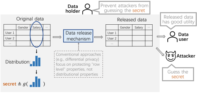
Figure 1: Problem overview. The data holder produces released data and wants to hide statistical secrets of the original data. The attacker (could be the data user) observes the released data, and wants to guess the secrets of the original data. We focus on secrets about the underlying distribution (e.g., mean, quantile, standard deviation of a specific data column). Many existing frameworks (e.g., differential privacy [16]) protect information from individual samples (rows).

Many widely-used privacy metrics and data sharing algorithms are not designed to protect summary statistic privacy, instead protecting the privacy of individual records in a database (e.g., differential privacy [16], anonymization [17], sub-sampling [17]). For example, differential privacy (DP) [16] evaluates how much individual samples influence the final output of an algorithm, and does not inherently protect summary statistics [9].

Many other frameworks have been designed specifically to hide aggregate properties of a dataset (or a distribution) [18, 19, 20]; we discuss these in detail in Section II. Many of these frameworks define privacy in terms of information-theoretic quantities such as mutual information [19] or other divergences [21]. In this work, we directly define the privacy of a mechanism as the posterior probability that a worst-case attacker can infer the data holder’s true secret after observing the released data. This definition is related to prior work analyzing min-entropy as a privacy metric [22]. To capture the utility of released data, we define the distortion of a mechanism as the worst-case Wasserstein-1 distance between the original and released data distributions. Our goal is to design data release mechanisms that efficiently trade off privacy and distortion (defined in III).

I-A Contributions

Our contributions are as follows.

• Lower bounds (§ IV): We derive general lower bounds on distortion given a privacy budget for any mechanism. These bounds depend on both the secret function and the data distribution. We derive closed-form lower bounds for a number of case studies (i.e., combinations of prior beliefs on the data distribution and secret functions).

• Mechanism design and upper bounds (§ V): We propose a class of mechanisms that achieve summary statistic privacy called quantization mechanisms, which intuitively quantize a data distribution’s parameters into bins. We show that for the case studies analyzed theoretically in Table I, the quantization mechanism achieves a privacy-distortion tradeoff within a small constant factor of optimal (usually $\leq$3) in the regime where quantization bins are small relative to the overall support set of the distribution parameters. We present a sawtooth technique for theoretically analyzing the quantization mechanism’s privacy tradeoff under various types of secret functions and data distributions (§ V-C). Intuitively, the sawtooth technique exploits the geometry of the distribution parameter(s) to divide the parametric space into two regions: one in which privacy risk is small and analytically tractable, and another in which privacy risk can be high, but which occurs with low probability. For the case studies that we do not analyze theoretically, we provide a dynamic programming algorithm that efficiently numerically instantiates the quantization mechanism.

• Empirical evaluation (§ VII): We give empirical results showing how to use summary statistic privacy to release a real dataset, and how to evaluate the corresponding summary statistic privacy metric. We show that the proposed quantization mechanism achieves better privacy-distortion tradeoffs than other related privacy mechanisms.

II Related Work

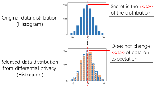
Figure 2: An illustrative example of why naive differential privacy mechanisms do not protect summary statistics. Assume that we want to protect the mean of the data. A typical differential privacy algorithm [23] would add zero-mean noise (e.g., Laplace noise) to the bins. This mechanism does not change the expected mean of the data.

We divide the related work into two categories: approaches based on indistinguishability over candidate inputs, and information-theoretic approaches.

II-A Indistinguishability-Based Approaches

Differential privacy (DP) [16] is one of the most commonly-adopted privacy frameworks. A random mechanism $\mathcal{M}{}$ is $(\epsilon,\delta)$-differentially-private if for any neighboring datasets $\mathcal{X}_{0}$ and $\mathcal{X}_{1}$ (i.e., $\mathcal{X}_{0}$ and $\mathcal{X}_{1}$ differ one sample), and any set $S\subseteq range\left(\mathcal{M}{}\right)$, we have

$$\mathbb{P}\left(\mathcal{M}\left(\mathcal{X}_{0}\right)\in S\right)\leq e^{\epsilon}\cdot\mathbb{P}\left(\mathcal{M}\left(\mathcal{X}_{1}\right)\in S\right)+\delta~{}~{}.$$

One could try to apply DP to our problem by treating $\mathcal{M}{}$ as the data release mechanism that reads the original dataset and outputs the released dataset. However, the threat models of DP and our framework are different: we want to hide functions of a distribution, while DP aims to hide whether any given sample contributed to the shared data. For example, when releasing the data in Fig. 2 as a histogram while preserving its mean, a typical DP algorithm [23] adds zero-mean noise (e.g., Laplace noise) to the bins. This process maintains the expected mean of the data, still allowing the attacker to derive an unbiased estimator of the mean from the released data.

A natural alternative is to devise a DP-like definition that explicitly protects the secret quantity. For instance, we could ask that for any pair of input distributions that differ in their secret quantity, the data release mechanism outputs similar released data distributions. Such an approach provides strong privacy guarantees, but may have poor utility. For instance, consider two Gaussian input distributions $\mathcal{N}\left(\mu_{1},\sigma_{1}^{2}\right)$ and $\mathcal{N}\left(\mu_{2},\sigma_{2}^{2}\right)$ with the secret as the mean. The values of $\sigma_{1}^{2}$ and $\sigma_{2}^{2}$ could be arbitrarily different. To make input distributions indistinguishable given the released data, we must destroy information about the true $\sigma$, which requires adding potentially unbounded noise. While relaxations like metric differential privacy may help [24], they may introduce new challenges, e.g., how to choose the metric function to map dataset distance to a privacy parameter.

Attribute privacy [18] tackles these challenges in part by constraining the space of distributions that should be indistinguishable [11]. Attribute privacy protects a function of a sensitive column in the dataset (named dataset attribute privacy) or a sensitive parameter of the underlying distribution from which the data is sampled (named distribution attribute privacy). It addresses the previously-mentioned shortcomings of vanilla DP under the pufferfish privacy framework [25]. Precisely, let $\mathcal{X}$ be the dataset, $\mathcal{G}$ be the possible range of a secret $g$, and $\mathcal{G}_{a},\mathcal{G}_{b}\subseteq\mathcal{G}$ be two non-overlapping subsets of the secret range $\mathcal{G}$. A mechanism $\mathcal{M}$ is $(\epsilon,\delta)$-attribute private if for any dataset $\mathcal{X}$, secret range pairs $\mathcal{G}_{a},\mathcal{G}_{b}$, and any set $S\subseteq range(\mathcal{M})$:

$$\mathbb{P}\left(\mathcal{M}(\mathcal{X})\in S|g(\mathcal{X})\in\mathcal{G}_{a}\right)\leq e^{\epsilon}\mathbb{P}\left(\mathcal{M}(\mathcal{X})\in S|g(\mathcal{X})\in\mathcal{G}_{b}\right)+\delta.$$

Attribute privacy focuses on algorithms that output a statistical query of the dataset instead of the entire dataset. Though we may apply attribute privacy to analyze full-dataset-sharing algorithms; it may need to add substantial noise due to the high dimensionality of the dataset (§ VII).

Distribution privacy [26] is a closely related notion, which releases a full data distribution under DP-style indistinguishability guarantees. Roughly, for any two input distributions with parameters $\theta_{0}$ and $\theta_{1}$ from a pre-defined set of candidate distributions, a distribution private mechanism outputs a distribution $\mathcal{M}(\theta_{i})$ for $i\in\{0,1\}$ such that for any set $S$ in the output space, we have $\mathbb{P}[\mathcal{M}(\theta_{i})\in S]\leq e^{\epsilon}\mathbb{P}[\mathcal{M}(\theta_{1-i})\in S]+\delta$. By obfuscating the whole distribution, distribution privacy inherently protects the private information. However the required noise may be more than what is needed to protect only select secret(s). For example, as mentioned above, two datasets can have exactly the same secret statistic (e.g., mean), while differing significantly in other respects (e.g., variance)—this requires significant noise in general. A recent work [27] proposes mechanisms for distribution privacy, and we observe this trend experimentally in § VII; the noise added by the mechanisms in [27] is larger than what we require with summary statistic privacy (though the privacy guarantees are different, so it is difficult to do a fair comparison).

Distribution inference [7, 8] considers a hypothesis test in which the adversary must choose whether released data comes from one of two fixed input data distributions $\omega_{1},\omega_{2}$. Both distributions are assumed to be known to all parties. By defining the attacker’s guessed distribution as $\hat{\omega}$ and attacker’s advantage as $\left|{\mathbb{P}\left(\hat{\omega}|\omega_{1}\right)-\mathbb{P}\left(\hat{\omega}|\omega_{2}\right)}\right|$, distribution inference aims to ensure that the attacker’s advantage is negligible. However, it is unclear how to establish a reasonable pair of candidate distributions; moreover, as with distribution privacy and attribute privacy, distribution inference may require high noise since it requires the data distributions to be indistinguishable.

II-B Information-Theoretic Approaches

The second category of frameworks use information-theoretic measures of privacy and utility [28, 29, 30, 31, 20, 32, 22, 33, 31, 34, 35, 36]. Such works often measure disclosure via divergences, such as mutual information [19, 31, 37, 38], $f$-divergences [21, 39], or min-entropy [29, 40, 30, 22, 41]. We discuss a few examples in detail here.

Privacy funnel [19] is a well-known information-theoretic privacy framework. Let $X$ be the random variable of the original data, containing sensitive information $U$, and let $Y$ represent the (random) released data. The privacy funnel framework evaluates privacy leakage with the mutual information $I(U;Y)$, and the utility of $Y$ with mutual information $I(X;Y)$. To find a data release mechanism $P_{Y|X}$, privacy funnel solves the optimization $\min_{P_{Y|X}:I(X;Y)\geq R}I(U;Y),$ where $R$ is a desired threshold on the utility of $Y$. Prior work has argued that mutual information is not a good metric for either privacy or utility [20]. On the privacy front, $I(U;Y)$ can be reduced while allowing the attacker to guess $S$ correctly from $Y$ with higher probability (see Example 1 in [20]). On the utility front, high mutual information $I(X;Y)$ does not mean that the released data $Y$ is a useful representation of $X$; $Y$ could be an arbitrary one-to-one transformation of $X$.

Maximal leakage [20] is an information-theoretic framework for quantifying the leakage of sensitive information. Using the same notation as before, the adversary’s guess of secret $U$ is denoted by $\hat{U}$. Based on this setup, the Markov chain $U-X-Y-\hat{U}$ holds. Maximal leakage $\mathcal{L}$ from $X$ to $Y$ is defined as

$$\mathcal{L}{}\left(X\to Y\right)=\sup_{U-X-Y-\hat{U}}\log\frac{\mathbb{P}\left(U=\hat{U}\right)}{\max_{u}P_{U}(u)},$$ (1)

where the $\sup$ is taken over $U$ (i.e., considering the worst-case secret) and $\hat{U}$ (i.e., considering the strongest attacker). Intuitively, Eq. 1 evaluates the ratio (in nats) of the probabilities of guessing the secret $U$ correctly with and without observing $Y$. Variants and generalizations of maximal leakage have been proposed, modifying Eq. 1 to penalize different values of $\mathbb{P}\left(U=\hat{U}\right)$ differently, using so-called gain functions [33, 34, 36, 35]. Maximal leakage and its variants assume that the secret $U$ is unknown a priori and therefore considers the worst-case leakage over all possible secrets. However, in our problem, data holders know what secret they want to protect.

Min-entropy metrics. Several papers have studied privacy metrics related to min-entropy, or the probability of guessing the secret correctly [29, 40, 30, 22, 41]. Among these, the most closely-related paper is by Asoodeh et al. [22], which directly analyzes the probability of guessing the secret, as we do (within a threshold). Adopting the same notation as before (i.e., the Markov chain $U-X-Y$), [22] aims to maximize the disclosure of $X$ (i.e., $\max_{f}\mathbb{P}\left(X=f(Y)\right)$, where the $\max$ is taken over all functions $f$) to ensure high utility. This optimization is subject to a privacy constraint on the sensitive information $U$: $\max_{\hat{g}}\mathbb{P}\left(U=\hat{g}(Y)\right)\leq T$, where the $\max$ is taken over all attack strategies $\hat{g}$. However, the authors assume that for random variables $X$ and $Y$, the value of each dimension can only be either $0$ or $1$ (i.e, each dimension of the data distribution parameter is binary). Since their analysis relies on the properties of Bernoulli distribution, the results cannot be trivially extended to non-binary case, significantly constraining the range of distribution settings this framework can analyze. Furthermore, they assess utility based on the probability of precisely guessing the original data. However, in data-sharing contexts, this utility measure suffers from the same shortcomings as mutual information, namely that any random one-to-one mapping can achieve a high utility metric without having practical utility.

III Problem Formulation

Notation.  We denote random variables with uppercase English letters or upright Greek letters (e.g., $X,\text{\textmugreek}$), and their realizations with italicized lowercase letters (e.g., $x,\mu$). For a random variable $X$, we denote its probability density function (PDF) as $f_{X}$, and its distribution measure as $\omega_{X}$. If a random variable $X$ is drawn from a parametric family (e.g., Gaussian with specified mean and covariance), the parameters will be denoted with a subscript of $X$, i.e., the above notations become $X_{\theta}$, $f_{X_{\theta}}$, $\omega_{X_{\theta}}$ respectively for parameters $\theta\in\mathbb{R}^{q}$, where $q\geq 1$ denotes the dimension of the parameters. In addition, we denote $f_{X|Y}$ as the conditional PDF or PMF of $X$ given another random variable $Y$. We use $\mathbb{Z},\mathbb{Z}_{>0},\mathbb{N},\mathbb{R},\mathbb{R}_{>0},$ to denote the set of integers, positive integers, natural numbers, real numbers, and positive real numbers respectively.

Original data.  Consider a data holder who possesses a dataset of $n$ samples $\mathcal{X}=\left\{x_{1},\ldots,x_{n}\right\}$, where for each $i\in[n]$, $x_{i}\in\mathbb{R}$ is drawn i.i.d. from an underlying distribution. We assume the distribution comes from a parametric family, and the parameter vector $\theta\in\mathbb{R}^{q}$ of the distribution fully specifies the distribution. That is, $x_{i}\sim\omega_{X_{\theta}}$, where we further assume that $\theta$ is itself a realization of random parameter vector $\Theta$, and $\omega_{\Theta}$ is the probability measure for $\Theta$. We will discuss how to relax the assumption on this prior distribution of $\theta$ in § VIII. We assume that the data holder knows $\theta$ (and hence knows its full data distribution $\omega_{X_{\theta}}$); our results and mechanisms generalize to the case when the data holder only possesses the dataset $\mathcal{X}$ (see § VI).

For example, suppose the original data samples come from a Gaussian distribution. We have $\theta=\left(\mu,\sigma\right)$, and $X_{\theta}\sim\mathcal{N}\left(\mu,\sigma\right)$. $\omega_{\Theta}$ (or $f_{\Theta}$) describes the prior distribution over $\left(\mu,\sigma\right)$. For example, if we know a priori that the mean of the Gaussian is drawn from a uniform distribution between 0 and 1, and $\sigma$ is always 1, we could have $f_{\Theta}\left(\mu,\sigma\right)=\mathbb{I}\left(\mu\in\left[0,1\right]\right)\cdot\delta\left(\sigma\right)$, where $\mathbb{I}\left(\cdot\right)$ is the indicator function, and $\delta$ is the Dirac delta function.

Statistical secret to protect.  We assume the data holder wants to hide a secret quantity, which is defined as a function of the original data distribution. Since the true data distribution is fully specified by parameter vector $\theta$, we define the secret as a function of $\theta$ as follows: $g\left(\theta\right):\mathbb{R}^{q}\to\mathbb{R}$. In the Gaussian example $X_{\theta}\sim\mathcal{N}\left(\mu,\sigma\right)$, suppose the data holder wishes to hide the mean; we thus have that $g\left({\mu,\sigma}\right)=\mu$.

Data release mechanism.  The data holder releases data by passing the private parameter $\theta$ through a data release mechanism $\mathcal{M}_{g}$. That is, for a given $\theta$, the data holder first draws internal randomness $z\sim\omega_{Z}$, and then releases another distribution parameter $\theta^{\prime}=\mathcal{M}_{g}\left(\theta,z\right)$, where $\mathcal{M}_{g}$ is a deterministic function, and $\omega_{Z}$ is a fixed distribution from which $z$ is sampled. Note that we assume both the input and output of $\mathcal{M}_{g}$ are distribution parameters. It is straightforward to generalize to the case when the input and/or output are datasets of samples (see § VI).

For example, in the Gaussian case discussed above, one data release mechanism could be $\mathcal{M}_{g}\left(\left(\mu,\sigma\right),z\right)=\left(\mu+z,\sigma\right)$ where $z\sim\mathcal{N}\left(0,1\right)$. I.e., the mechanism shifts the mean by a random amount drawn from a standard Gaussian distribution and keeps the variance.

Threat model.  We assume that the attacker knows the parametric family from which our data is drawn, and has a prior over the parameter realization, but does not know the initial parameter $\theta$. The attacker is also assumed to know the data release mechanism $\mathcal{M}_{g}$ and output $\theta^{\prime}$ but not the realization of the data holder’s internal randomness $z$. The attacker guesses the initial secret $g\left(\theta\right)$ based on the released parameter $\theta^{\prime}$ according to estimate $\hat{g}\left(\theta^{\prime}\right)$. $\hat{g}$ can be either random or deterministic, and we assume no computational bounds on the adversary. For instance, in the running Gaussian example, an attacker may choose $\hat{g}\left({\mu^{\prime},\sigma^{\prime}}\right)=\mu^{\prime}$. When the data holder releases a dataset of samples instead of the parameter $\theta^{\prime}$, this formulation can be used to upper bound the attacker’s performance on correctly guessing the secret, since the estimation error on released distribution parameter is induced due to the finite samples in the released dataset.

Privacy metric.  The data holder wishes to prevent an attacker from guessing its secret $g\left(\theta\right)$. We define our privacy metric privacy $\Pi_{\epsilon,\omega_{\Theta}}{}$ as the attacker’s probability of guessing the secret(s) to within a tolerance $\epsilon$, taken worst-case over all attackers $\hat{g}$:

$$\Pi_{\epsilon,\omega_{\Theta}}{}\triangleq~{}\sup_{\hat{g}}~{}\mathbb{P}\left(\lvert\hat{g}\left(\theta^{\prime}\right)-g\left(\theta\right)\rvert\leq\epsilon\right)~{}.$$ (2)

The probability is taken over the randomness of the original data distribution ($\theta\sim\omega_{\Theta}$), the data release mechanism ($z\sim\omega_{Z}$), and the attacker strategy ($\hat{g}$).

Distortion metric.  The main goal of data sharing is to provide useful data; hence, we (and data holders and users) want to understand how much the released data distorts the original data. We define the distortion $\Delta$ of a mechanism as the worst-case distance between the original distribution and the released distribution:

$$\Delta\triangleq\sup_{\begin{subarray}{c}\theta\in\text{Supp}\left(\omega_{\Theta}\right),\theta^{\prime},\\ z\in\text{Supp}\left(\omega_{Z}\right):\mathcal{M}_{g}\left(\theta,z\right)=\theta^{\prime}\end{subarray}}d\left(\omega_{X_{\theta}}\|\omega_{X_{\theta^{\prime}}}\right),$$ (3)

where $d$ is

Wasserstein-1 distance. Wasserstein-1 distance is commonly used as the distance metric in neural network design (e.g., [42, 43]). Note that the definition in Eq. 3 can be extended to data release mechanisms that take datasets as inputs and/or outputs.

Formulation.  To summarize, the data holder’s objective is to choose a data release mechanism that minimizes distortion $\Delta{}$ subject to a constraint on privacy $\Pi_{\epsilon,\omega_{\Theta}}{}$:

$$\begin{split}\min_{\mathcal{M}_{g}}&\qquad\Delta{}\\ \text{subject to}&\qquad\Pi_{\epsilon,\omega_{\Theta}}\leq T.\end{split}$$ (4)

The reverse formulation, $\min_{\mathcal{M}_{g}}\Pi_{\epsilon,\omega_{\Theta}}{}~{}~{}\text{subject to}~{}~{}\Delta\leq T$ is analyzed in Appendix A.

The optimal data release mechanisms for Eq. 4 depends on the secrets and the characteristics of the original data. Data holders specify the secret function they want to protect and select the data release mechanism to process the raw data for sharing.

Our goal is to study: (1) What are fundamental limits on the tradeoff between privacy and distortion? (2) Do there exist data release mechanisms that can match or approach these fundamental limits? In general, these questions can have different answers for different parametric families of data distributions and secret functions. In § IV and § V, we first present general results that do not depend on data distribution or secret function. We then present case studies for specific secret functions and data distributions in § VI.

IV General Lower Bound on Privacy-Distortion Tradeoffs

Given a privacy budget $T$, we first present a lower bound on distortion that applies regardless of the prior distribution of data $\omega_{\Theta}$ and regardless of the secret $g$.

Theorem 1 (Lower bound of privacy-distortion tradeoff).

Let $D\left(X_{\theta_{1}},X_{\theta_{2}}\right)\triangleq\frac{1}{2}d\left(\omega_{X_{\theta_{1}}}\|\omega_{X_{\theta_{2}}}\right)$, where $d\left(\cdot\|\cdot\right)$ denotes Wasserstein-1 distance. Further, let $R\left(X_{\theta_{1}},X_{\theta_{2}}\right)\triangleq\lvert g{({{\theta_{1}}})-g{({{\theta_{2}}})}}\rvert$ and

$$\ratio\triangleq\inf_{\theta_{1},\theta_{2}\in\text{Supp}\left(\omega_{\Theta}\right)}\frac{D\left(X_{\theta_{1}},X_{\theta_{2}}\right)}{R\left(X_{\theta_{1}},X_{\theta_{2}}\right)}.$$ (5)

For any $T\in\left(0,1\right)$, when $\Pi_{\epsilon,\omega_{\Theta}}\leq T$,

$$\Delta>\left(\lceil{\frac{1}{T}}\rceil-1\right)\cdot 2\ratio\epsilon~{}.$$ (6)

The proof is shown as below. From Theorem 1 we see that the lower bound of distortion scales inversely with the privacy budget and positively with the tolerance threshold $\epsilon$. The dependent quantity $\gamma$ in Eq. 5 can be thought of as a conversion factor that bounds the translation from probability of detection to distributional distance. Note that we have not made exact as its form depends on the type of the secret and prior distribution of data. We will instantiate it in the cases studies in § VI.

Proof.

Our proof proceeds by constructing an ensemble of attackers, such that at least one of them will be correct by construction. We do this by partitioning the space of possible secret values, and having each attacker output the midpoint of one of the subsets of the partition. We then use the fact that each attacker can be correct with probability at most $T$, combined with $\gamma$, which intuitively relates the distance between distributions to the distance between their secrets, to derive the claim. Recall that $\theta$ is the true private parameter vector, $\theta^{\prime}$ is the released parameter vector as a result of the data release mechanism.

$$T \geq\Pi_{\epsilon,\omega_{\Theta}}$$

$$=\sup_{\hat{g}}\mathbb{P}\left(\hat{g}\left(\theta^{\prime}\right)\in\left[g\left(\theta\right)-\epsilon,g\left(\theta\right)+\epsilon\right]\right)$$

$$=\sup_{\hat{g}}\mathbb{E}\left(\mathbb{P}\left(\hat{g}\left(\theta^{\prime}\right)\in\left[g\left(\theta\right)-\epsilon,g\left(\theta\right)+\epsilon\right]\bigg{|}\theta^{\prime}\right)\right)$$

$$=\mathbb{E}\left(\sup_{\hat{g}}\mathbb{P}\left(\hat{g}\left(\theta^{\prime}\right)\in\left[g\left(\theta\right)-\epsilon,g\left(\theta\right)+\epsilon\right]\bigg{|}\theta^{\prime}\right)\right)~{}~{},$$ (7)

where Eq. 7 is due to the following facts: (1) LHS $\leq$ RHS because
$\sup_{\hat{g}}\mathbb{P}\left(\hat{g}\left(\theta^{\prime}\right)\in\left[g\left(\theta\right)-\epsilon,g\left(\theta\right)+\epsilon\right]\bigg{|}\theta^{\prime}\right)\geq\mathbb{P}\left(\hat{g}\left(\theta^{\prime}\right)\in\left[g\left(\theta\right)-\epsilon,g\left(\theta\right)+\epsilon\right]\bigg{|}\theta^{\prime}\right)$ for any $\theta^{\prime}$; (2) RHS $\leq$ LHS because $\hat{g}$ can only depend on $\theta^{\prime}$. Therefore, we can map any $\arg\sup_{\hat{g}}$ in the RHS to the LHS and obtain the same value, since the expectation is taken over $\theta^{\prime}$. Thus, there exists $\theta^{\prime}$ s.t. $\sup_{\hat{g}}\mathbb{P}\left(\hat{g}\left(\theta^{\prime}\right)\in\left[g\left(\theta\right)-\epsilon,g\left(\theta\right)+\epsilon\right]\bigg{|}\theta^{\prime}\right)\leq T$. Let

$$L_{\theta^{\prime}}\triangleq\inf_{\theta\in\text{Supp}\left(\omega_{\Theta}\right),z:\mathcal{M}_{g}\left(\theta,z\right)=\theta^{\prime}}g\left(\theta\right)~{},$$

$$R_{\theta^{\prime}}\triangleq\sup_{\theta\in\text{Supp}\left(\omega_{\Theta}\right),z:\mathcal{M}_{g}\left(\theta,z\right)=\theta^{\prime}}g\left(\theta\right)~{}.$$

We can define a sequence of attackers and a constant $N$ such that $\hat{g}_{i}\left(\theta^{\prime}\right)=L_{\theta^{\prime}}+\left(i+0.5\right)\cdot 2\epsilon$ for $i\in\left\{0,1,\ldots,N-1\right\}$ and $L_{\theta^{\prime}}+2N\epsilon\geq R_{\theta^{\prime}}>L_{\theta^{\prime}}+2(N-1)\epsilon$ (Fig. 3).

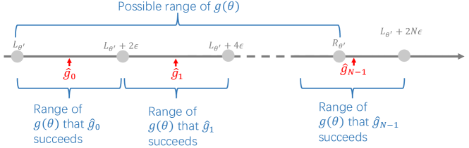
Figure 3: The construction of attackers for proof of Theorem 1. The $2\epsilon$ ranges of $\hat{g}_{0},...,\hat{g}_{N-1}$ jointly cover the entire range of possible secret $\left[L_{\theta^{\prime}},R_{\theta^{\prime}}\right]$. The probability of guessing the secret correctly for any attacker is $\leq T$. Therefore, $R_{\theta^{\prime}}-L_{\theta^{\prime}}>\left(\lceil{\frac{1}{T}}\rceil-1\right)\cdot 2\epsilon$ (Eq. 8).

From the above, we have

$$T\cdot N\geq\sum_{i}\mathbb{P}\left(\hat{g}_{i}\left(\theta^{\prime}\right)\in\left[g\left(\theta\right)-\epsilon,g\left(\theta\right)+\epsilon\right]\bigg{|}\theta^{\prime}\right)\geq 1,$$

Therefore, we have $N\geq\lceil{\frac{1}{T}}\rceil$, and

$$R_{\theta^{\prime}}-L_{\theta^{\prime}}>\left(\lceil{\frac{1}{T}}\rceil-1\right)\cdot 2\epsilon~{}~{}.$$ (8)

Then we have

$$\Delta \geq\sup_{\theta\in\text{Supp}\left(\omega_{\Theta}\right),z\in\text{Supp}\left(\omega_{Z}\right):\mathcal{M}_{g}\left(\theta,z\right)=\theta^{\prime}}d\left(\omega_{X_{\theta}}\|\omega_{X_{\theta^{\prime}}}\right)$$

$$\geq\sup_{\theta_{i}\in\text{Supp}\left(\omega_{\Theta}\right),z_{i}:\mathcal{M}_{g}\left(\theta_{i},z_{i}\right)=\theta^{\prime}}D\left(X_{\theta_{1}},X_{\theta_{2}}\right)$$ (9)

$$>\left(\lceil{\frac{1}{T}}\rceil-1\right)\cdot 2\ratio\epsilon.$$ (10)

where in Eq. 9, $\theta_{i}$ for $i\in\{1,2\}$ denotes two arbitrary parameter vectors in the support space, and Eq. 9 comes from the triangle inequality, and Eq. 10 utilizes $R_{\theta^{\prime}}-L_{\theta^{\prime}}>\left(\lceil{\frac{1}{T}}\rceil-1\right)\cdot 2\epsilon$ and the definition of . ∎

V Data Release Mechanisms

We first present in § V-A the quantization mechanism, a template for data release mechanisms used in the case studies of § VI. The quantization mechanism can be instantiated differently for different secret functions and data distributions. We show in § V-B techniques for instantiating the quantization mechanism, either based on theoretical insights or numerically. Finally, we give some intuition in § V-C about how to analyze the quantization mechanism. These insights will be used in our case studies (§ VI) to show that we can sometimes match the lower bounds from § IV up to small constant factors.

V-A The Quantization Mechanism

At a high level, the quantization mechanisms follow two steps:

1. Offline Phase: Partition the space of parameters $\text{Supp}\left(\Theta\right)$ into carefully-chosen bins.

2. Online Phase: For an observed data distribution parameter $\theta$, deterministically release the quantized parameters, according to the partition from the Offline Phase.

More precisely, we first divide the set of possible distribution parameters $\text{Supp}\left(\Theta\right)$ into subsets $\mathcal{S}_{i}$ such that $\cup_{i\in\mathcal{I}}\mathcal{S}_{i}\supseteq\text{Supp}\left(\Theta\right)$ and $\mathcal{S}_{i_{1}}\cap\mathcal{S}_{i_{2}}=\emptyset$ for $i_{1}\not=i_{2}$, where $\mathcal{I}$ is the (possibly uncountable) set of indices of the subsets. For $\theta\in\text{Supp}\left(\Theta\right)$, $I\left(\theta\right)$ is the index of the set that $\theta$ belongs to; in other words, we have $I\left(\theta\right)=i$, where $\theta\in\mathcal{S}_{i}$. The mechanism first looks up which set $\theta$ belongs to (i.e., $I\left(\theta\right)$), then deterministically releases a parameter $\theta^{*}_{I\left(\theta\right)}$ that corresponds to the set. Here, $\theta^{*}_{i}$ for $i\in\mathcal{I}$ denotes another parameter. In short, our data release mechanism has the form

$$\mathcal{M}_{g}\left(\theta,z\right)=\theta^{*}_{I\left(\theta\right)}~{}~{}.$$

Note that the policy is fully determined by $\mathcal{S}_{i}$ and $\theta^{*}_{i}$. In the remainder of the paper, we will show different ways of instantiating quantization mechanism to approach the lower bound in § IV.

Intuitively, quantization mechanisms will have a bounded distortion as long as $d\left(\omega_{X_{\theta}}\|\omega_{X_{\theta^{*}_{I\left(\theta\right)}}}\right)$ is bounded for all $\theta\in\text{Supp}\left(\Theta\right)$. At the same time, they obfuscate the secret as different data distributions within the same set are mapped to the same released parameter. It turns out this simple deterministic mechanism is sufficient to achieve the (order) optimal privacy-distortion trade-offs in many cases, as opposed to differential privacy, which requires randomness to provide theoretical guarantees [16] (examples in the case studies § VI).

V-B Algorithms for Instantiating the Quantization Mechanism

To implement the quantization mechanism, we need to define the quantization bins $\mathcal{S}_{i}$ and the released parameter per bin $\theta^{*}_{i}$. Depending on the data distribution, the secret function, and quantization mechanism parameters, the mechanism can have very different privacy-distortion tradeoffs. We present two methods for selecting quantization parameters: (1) an analytical approach, and (2) a numeric approach.

Analytical approach (sketch)

In some cases, outlined in the case studies of § VI and the appendices, we can find analytical expressions for $\mathcal{S}_{i}$ and $\theta^{*}_{i}$ while (near-)optimally trading off privacy for distortion. This is usually possible when the lower bound depends on the problem parameters in a specific way (see below). We will next illustrate the procedure through an example; precise analysis is given in §VI.

For example, for the Gaussian distribution where $\theta=\left(\mu,\sigma\right)$, when secret=standard deviation, we can work out the lower bound from Theorem 1 (details in Appendix G). Note that the lower bound is tight if our mechanism minimizes

$$\frac{D\left(X_{\mu_{1},\sigma_{1}},X_{\mu_{2},\sigma_{2}}\right)}{R\left(X_{\mu_{1},\sigma_{1}},X_{\mu_{2},\sigma_{2}}\right)}=\sqrt{\frac{1}{2\pi}}e^{-\frac{1}{2}\left(\frac{\mu_{1}-\mu_{2}}{\sigma_{1}-\sigma_{2}}\right)^{2}}-\left(\frac{\mu_{1}-\mu_{2}}{\sigma_{1}-\sigma_{2}}\right)\left(\frac{1}{2}-\Phi\left(\left(\frac{\mu_{1}-\mu_{2}}{\sigma_{1}-\sigma_{2}}\right)\right)\right)$$ (11)

where where $D\left(X_{\theta_{1}},X_{\theta_{2}}\right)$ and $R\left(X_{\theta_{1}},X_{\theta_{2}}\right)$ are defined in Theorem 1, and $\Phi$ denotes the CDF of the standard Gaussian distribution. That is, for any true parameters $\mu_{1}$ and $\sigma_{1}$, the mechanism should always choose to release $\mu_{2}$ and $\sigma_{2}$ such that Eq. 11 is as small as possible. The exact form of Eq. 11 is not important for now; notice instead that the problem parameters $(\sigma_{i},\mu_{i})$ take the same form every time they appear in this equation. We define $t(\theta_{1},\theta_{2})=\frac{\mu_{1}-\mu_{2}}{\sigma_{1}-\sigma_{2}}$ to be that form. Next, we find the $t(\theta_{1},\theta_{2})$ that minimizes Eq. 11:

$$t_{0}\triangleq\underset{t(\theta_{1},\theta_{2})}{\arg\inf}\ \frac{D\left(X_{\theta_{1}},X_{\theta_{2}}\right)}{R\left(X_{\theta_{1}},X_{\theta_{2}}\right)}$$

For instance, in our Gaussian example, we can write $t_{0}$ as

$$t_{0}=\underset{t(\theta_{1},\theta_{2})}{\arg\inf}\sqrt{\frac{1}{2\pi}}e^{-\frac{1}{2}\left(t(\theta_{1},\theta_{2})\right)^{2}}-\left(t(\theta_{1},\theta_{2})\right)\left(\frac{1}{2}-\Phi\left(t(\theta_{1},\theta_{2})\right)\right),$$

which can be solved numerically. Finally, we can choose $\mathcal{S}_{i}$ and $\theta^{*}_{i}$ to be sets for which $t\left(\theta,\theta^{*}_{i}\right)=t_{0},\ \forall\theta\in\mathcal{S}_{i}.$ Using this rule, we derive the mechanism:

$$\mathcal{S}_{\mu,i} =\left\{\left(\mu+t_{0}\cdot t,\underline{\sigma}+\left(i+0.5\right)\cdot s+t\right)|t\in\left[-\frac{s}{2},\frac{s}{2}\right)\right\}~{}~{},$$

$$\theta^{*}_{\mu,i} =\left(\mu,\underline{\sigma}+\left(i+0.5\right)\cdot s\right)~{}~{},$$

$$\mathcal{I} =\left\{\left(\mu,i\right)|i\in\mathbb{N},\mu\in\mathbb{R}\right\},$$

where $s$ is a hyper-parameter of the mechanism that divides $\left(\overline{\sigma}-\underline{\sigma}\right)$, and $\overline{\sigma},\underline{\sigma}$ are upper and lower bounds on $\sigma$, determined by the adversary’s prior.

For our Gaussian example, the resulting sets $\mathcal{S}_{\mu,i}$ for the quantization mechanism are shown in Fig. 4; the space of possible parameters is divided into infinitely many subsets $\mathcal{S}_{\mu,i}$, each consisting of a diagonal line segment (parallel blue lines in Fig. 4). The space of possible $\sigma$ values is divided into segments of length $s$, which correspond to the horizontal bands in Fig. 4. Given this choice of intervals, the mechanism proceeds as follows: when the true distribution parameters fall in one of these intervals, the mechanism releases the midpoint of the interval. The fact that the intervals $\mathcal{S}_{\mu,i}$ are diagonal lines arises from choosing $t(\theta_{1},\theta_{2})=\frac{\mu_{1}-\mu_{2}}{\sigma_{1}-\sigma_{2}}$; each interval corresponds to a set of points $(\tilde{\mu},\tilde{\sigma})$ that satisfy $t(\theta_{1},\theta_{2})=t_{0}$, i.e., with slope $1/t_{0}$.

We will see how to use this construction to obtain upper bounds on privacy-distortion tradeoffs in § V-C.

Numeric approach

In some cases, the above procedure may not be possible. To this end, we present a dynamic programming algorithm to numerically compute the quantization mechanism parameters. This algorithm achieves an optimal privacy-distortion tradeoff [44] among the class of quantization algorithms with finite precision and continuous intervals $\mathcal{S}_{i}$. We use this algorithm in some of the case studies in § VI. We present our dynamic programming algorithm for univariate data distributions.

We assume $\text{Supp}\left(\Theta\right)=\left[\underline{\theta},\overline{\theta}\right)$, where $\underline{\theta},\overline{\theta}$ are lower and upper bounds of $\theta$, respectively. We consider the class of quantization mechanisms such that $\mathcal{S}_{i}=\left[\underline{\theta^{i}},\overline{\theta^{i}}\right)$, i.e., each subset of parameters are in a continuous range. Furthermore, we explore mechanisms such that $\underline{\theta^{i}},\overline{\theta^{i}},\theta^{*}_{i}\in\left\{\underline{\theta},\underline{\theta}+\kappa,\underline{\theta}+2\kappa,\ldots,\overline{\theta}\right\}$, where $\kappa$ is a hyper-parameter that encodes numeric precision (and therefore divides $(\overline{\theta}-\underline{\theta})$). For example, if we want to hide the mean of a Geometric random variable with $\underline{\theta}=0.1$ and $\overline{\theta}=0.9$, we could consider three-decimal-place precision, i.e., $\kappa=0.001$ and $\underline{\theta^{i}},\overline{\theta^{i}},\theta^{*}_{i}\in\left\{0.100,0.101,0.102,\ldots,0.900\right\}$.

Since $\Delta$ (Eq. 3) is defined as the worst-case distortion whereas $\Pi_{\epsilon,\omega_{\Theta}}$ (Eq. 2) is defined as a probability, which is related to the original data distribution, optimizing $\Pi_{\epsilon,\omega_{\Theta}}$ given bounded $\Delta$ (Eq. 12) is easier to solve than the final goal of optimizing $\Delta$ given bounded $\Pi_{\epsilon,\omega_{\Theta}}$ (Eq. 4).

$$\begin{split}\min_{\mathcal{M}_{g}}~{}~{}\Pi_{\epsilon,\omega_{\Theta}}{}\quad\quad\quad\text{subject to}~{}~{}\Delta\leq T.\end{split}$$ (12)

Observing that in Eq. 4 the optimal value of $\min_{\mathcal{M}_{g}}\Delta{}$ is a monotonic decreasing function w.r.t. the threshold $T$, we can use a binary search algorithm (shown in Appendix B) to reduce problem Eq. 4 to problem Eq. 12. It calls an algorithm that finds the optimal quantization mechanism with numerical precision over continuous intervals under a distortion budget $T$ (i.e., solving Eq. 12). This problem can be solved by a dynamic programming algorithm. Let $pri\left(t^{*}\right)$ ($t^{*}\in\left\{\underline{\theta},\underline{\theta}+\kappa,\underline{\theta}+2\kappa,\ldots,\overline{\theta}\right\}$) be the minimal privacy $\Pi_{\epsilon,\omega_{\Theta}}{}$ we can get for $\text{Supp}\left(\Theta\right)=\left\{X_{\theta}:\theta\in\left[\underline{\theta},t^{*}\right)\right\}$ such that $\Delta\leq T$. Denote $\mathcal{D}\left(\theta_{1},\theta_{2}\right)$ as the minimal distortion a quantization mechanism can achieve under the quantization bin $\left[\theta_{1},\theta_{2}\right)$, we have

$$\mathcal{D}\left(\theta_{1},\theta_{2}\right)=\inf_{\theta\in\mathbb{R}^{q}}\sup_{\theta^{\prime\prime}\in\left[\theta_{1},\theta_{2}\right)}d\left(\omega_{X_{\theta^{\prime\prime}}}\|\omega_{X_{\theta}}\right),$$

where $d\left(\cdot\|\cdot\right)$ is defined in Eq. 3. We also denote $\mathcal{D}^{*}\left(\theta_{1},\theta_{2}\right)=\arg\inf_{\theta\in\left[\theta_{1},\theta_{2}\right)}\sup_{\theta^{\prime\prime}\in\left[\theta_{1},\theta_{2}\right)}d\left(\omega_{X_{\theta^{\prime\prime}}}\|\omega_{X_{\theta}}\right)$. If the prior over parameters is $f_{\Theta}$, we have the Bellman equation

$$pri\left(t^{*}\right)=\min_{\theta\in\left[\underline{\theta},t^{*}-\kappa\right],\mathcal{D}\left(\theta,t^{*}\right)\leq T}\frac{\int_{\underline{\theta}}^{\theta}f_{\Theta}\left(t\right)\mathrm{d}t}{\int_{\underline{\theta}}^{t^{*}}f_{\Theta}\left(t\right)\mathrm{d}t}\cdot pri\left(\theta\right)+\frac{\int_{\theta}^{t^{*}}f_{\Theta}\left(t\right)\mathrm{d}t}{\int_{\underline{\theta}}^{t^{*}}f_{\Theta}\left(t\right)\mathrm{d}t}\cdot\mathcal{P}\left(\theta,t^{*}\right)$$

with the initial state $pri\left(\underline{\theta}\right)=0$, where

$$\mathcal{P}\left(\theta,t^{*}\right) =\mathbb{P}\left(\hat{g}^{*}\left(\theta^{\prime}\right)\in\left[g\left(\theta_{0}\right)-\epsilon,g\left(\theta_{0}\right)+\epsilon\right]|\theta_{0}\in\left[\theta,t^{*}\right],\theta^{\prime}\right)$$

$$=\sup_{t_{1},t_{2}:\ \sup_{t^{\prime},t^{\prime\prime}\in\left[t_{1},t_{2}\right]}\lvert g\left(t^{\prime\prime}\right)-g\left(t^{\prime}\right)\rvert=2\epsilon}\frac{\int_{\max{\left\{t_{1},\theta\right\}}}^{\min{\left\{t_{2},t^{*}\right\}}}f_{\Theta}\left(t\right)\mathrm{d}t}{\int_{\theta}^{t^{*}}f_{\Theta}\left(t\right)\mathrm{d}t}.$$

$\theta^{\prime}$ is the released parameter when the private parameter $\theta_{0}\in\left[\theta,t^{*}\right]$ and $\hat{g}^{*}$ is the optimal attack strategy. The full algorithm is listed in Algorithm 1. The time complexity of this algorithm is $\mathcal{O}\left(\left(\nicefrac{{\overline{\theta}-\underline{\theta}}}{{\kappa}}\right)^{2}\cdot\mathcal{C}_{D}\cdot\mathcal{C}_{P}\cdot\mathcal{C}_{I}\right)$, where $\mathcal{C}_{D}$ is the time complexity for computing $\mathcal{D}$ and $\mathcal{D}^{*}$, $\mathcal{C}_{P}$ is the time complexity for computing $\mathcal{P}$, and $\mathcal{C}_{I}$ is the time complexity for computing the integrals in the Bellman equation. In our cases studies, $\mathcal{D}$ and $\mathcal{D}^{*}$ can be computed in $\mathcal{C}_{D}=\mathcal{O}\left(\nicefrac{{\overline{\theta}-\underline{\theta}}}{{\kappa}}\right)$, and $\mathcal{P}$ and the integrals can be computed in closed forms within constant time, i.e., $\mathcal{C}_{P}=\mathcal{C}_{I}=\mathcal{O}\left(1\right)$.

Input : Parameter range: $\left[\underline{\theta},\overline{\theta}\right)$

Prior over parameter: $f_{\Theta}$

Distortion budget: $T$

Step size: $\kappa$ (which divides $\overline{\theta}-\underline{\theta}$)

1 $pri(\underline{\theta})\leftarrow 0$

2 $\mathcal{I}\left(\underline{\theta}\right)\leftarrow\emptyset$

3

4for $t^{*}{}\leftarrow\underline{\theta}+\kappa,\underline{\theta}+2\kappa,\ldots,\overline{\theta}$ do

5       $pri(t^{*})\leftarrow\infty$

6       $min\_t\leftarrow$ NULL

7       for $\theta\leftarrow t^{*}-\kappa,\ldots,\underline{\theta}$ do

8             if $\mathcal{D}\left(\theta,t^{*}\right)>T$ then

9                  break

10            $p\leftarrow\frac{\int_{\underline{\theta}}^{\theta}f_{\Theta}\left(t\right)\mathrm{d}t}{\int_{\underline{\theta}}^{t^{*}}f_{\Theta}\left(t\right)\mathrm{d}t}\cdot pri\left(\theta\right)+\frac{\int_{\theta}^{t^{*}}f_{\Theta}\left(t\right)\mathrm{d}t}{\int_{\underline{\theta}}^{t^{*}}f_{\Theta}\left(t\right)\mathrm{d}t}\cdot\mathcal{P}\left(\theta,t^{*}\right)$

11             if $p<pri(t^{*})$ then

12                   $pri(t^{*})\leftarrow p$

13                   $min\_t\leftarrow\theta$

14            

15      if $min\_t$ is not NULL then

16             $\mathcal{S}_{t^{*}}\leftarrow\left[min\_t,~{}t^{*}\right)$

17             $\theta^{\prime}_{t^{*}}\leftarrow\mathcal{D}^{*}\left(min\_t,t^{*}\right)$

18             $\mathcal{I}\left(t^{*}\right)\leftarrow\mathcal{I}\left(min\_t\right)\cup\left\{t^{*}\right\}$

19            

20      

21if $pri(\overline{\theta})=\infty$ then

22      ERROR: No answer

return $pri(\overline{\theta})$, $\left\{\mathcal{S}_{i}:i\in\mathcal{I}\left(\overline{\theta}\right)\right\},\left\{\theta^{\prime}_{i}:i\in\mathcal{I}\left(\overline{\theta}\right)\right\}$

Algorithm 1 Dynamic-programming-based data release mechanism for single-parameter distributions.

When dynamic programming is not practical (e.g., in high-dimensional problems), we also provide a greedy algorithm in Appendix B as a baseline and show the empirical comparison between these two algorithms in the case studies (Appendices E, G and H).

V-C Technique for Analyzing the Quantization Mechanism

We next provide an overview of techniques for analyzing the quantization mechanism, both for privacy and for distortion. We use these techniques for the analysis in our case studies, where we will make the expressions and claims more precise. For concreteness, we will recall the Gaussian example from § V-B, for which we have already derived a mechanism.

The mechanism presented in § V-B can geometrically be interpreted as follows. Over the square of possible parameter values $\mu$ and $\sigma$ (Fig. 4), the mechanism selects intervals $\mathcal{S}_{\mu,i}$ that consist of short diagonal line segments (e.g., blue line segments in Fig. 4). When the true distribution parameters fall in one of these intervals, the mechanism releases the midpoint of the interval.

We find that many of our case studies naturally give rise to the same form of $t(\theta)$. As a result, all of the case studies we analyze theoretically (with multiple parameters) have mechanisms that instantiate intervals $\mathcal{S}_{\mu,i}$ as diagonal lines, as shown in Fig. 4. The sawtooth technique, which we present next, can be used to analyze the privacy of all such mechanism instantiations. More precisely, the following pattern of quantization mechanism admits diagonal line intervals, and can be analyzed with the sawtooth technique (§ VI, E and G):

$$\mathcal{S}_{\mu,i} =\left\{\left(\mu+t_{0}\cdot t,\underline{\sigma}+\left(i+0.5\right)\cdot s+t\right)|t\in\left[-\frac{s}{2},\frac{s}{2}\right)\right\}~{}~{},$$

$$\theta^{*}_{\mu,i} =\left(\mu,\underline{\sigma}+\left(i+0.5\right)\cdot s\right)~{}~{},$$

$$\mathcal{I} =\left\{\left(\mu,i\right)|i\in\mathbb{N},\mu\in\mathbb{R}\right\},$$

where $s$ is a hyper-parameter of the mechanism that denotes quantization bin size and divides $\left(\overline{\sigma}-\underline{\sigma}\right)$ and $t_{0}$ is a constant that can be determined by the mechanism design strategy described in § V-B.

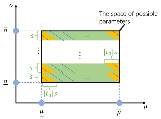
Figure 4: We separate the space of possible parameters into two regions (yellow and green) and bound the attacker’s success rate on each region separately. The blue lines represent examples of $\mathcal{S}_{\mu,i}$.

(1) Privacy analysis.  For ease of illustration, we assume that the support of parameters is $\text{Supp}\left(\Theta\right)=\left\{(a,b)|a\in\left[\underline{\mu},\overline{\mu}\right),b\in\left[\underline{\sigma},\overline{\sigma}\right)\right\}$, but the analysis can be generalized to any case.

In Fig. 4, we separate the space of possible data parameters into two regions represented by yellow and green colors. The yellow regions $S_{yellow}$ constitute right triangles with height $s$ and width $\lvert t_{0}\rvert s$. The green region $S_{green}$ is the rest of the parameter space. The high-level idea of our proof is as follows. Note that for any parameter $\theta\in S_{green}$, there exists a quantization bin $\mathcal{S}_{\mu,i}$ s.t. $\theta\in\mathcal{S}_{\mu,i}$ and $\mathcal{S}_{\mu,i}\subset S_{green}$. This occurs because the mechanism intervals (blue lines in Fig. 4) all have the same slope and a length of at most $s$ for $\sigma$. As such, each interval is either fully in the green region, or fully in the yellow region. Since we know the length of each bin, we can upper bound the attack success rate if $\theta\in S_{green}$. While the attacker can be more successful in the yellow region, the probability of $\theta\in S_{yellow}$ is small. Hence, we upper bound the overall attacker’s success rate (i.e., $\Pi_{\epsilon,\omega_{\Theta}}$). More specifically, let the optimal attacker be $\hat{g}^{*}$. We have

$$\Pi_{\epsilon,\omega_{\Theta}}{} =\mathbb{P}\left(\hat{g}^{*}\left(\theta^{\prime}\right)\in\left[g\left(\theta\right)-\epsilon,g\left(\theta\right)+\epsilon\right]\right)$$

$$=\int_{\theta\in S_{green}}p(\theta)\mathbb{P}\left(\hat{g}^{*}\left(\theta^{\prime}\right)\in\left[g\left(\theta\right)-\epsilon,g\left(\theta\right)+\epsilon\right]\right)d\theta$$

$$\quad+\int_{\theta\in S_{yellow}}p(\theta)\mathbb{P}\left(\hat{g}^{*}\left(\theta^{\prime}\right)\in\left[g\left(\theta\right)-\epsilon,g\left(\theta\right)+\epsilon\right]\right)d\theta$$

$$<\sup_{\theta\in S_{green}}\mathbb{P}\left(\hat{g}^{*}\left(\theta^{\prime}\right)\in\left[g\left(\theta\right)-\epsilon,g\left(\theta\right)+\epsilon\right]\right)+\int_{\theta\in S_{yellow}}p(\theta)d\theta$$

The first term can be bounded away from 1 due to the carefully chosen $t_{0}$. The second term is bounded away from 1 because the size of $S_{yellow}$ is relatively small. The formal justification is given in Propositions 2, C-D2, F-B and G-D.

(2) Distortion analysis.  For the distortion performance, it is straightforward to show that
$\Delta=\sup_{\theta\in\text{Supp}\left(\Theta\right)}d\left(\omega_{X_{\theta}}\|\omega_{X_{\theta^{*}_{I\left(\theta\right)}}}\right)$, where $\theta^{*}_{I\left(\theta\right)}$ is the released parameter when the original parameter is $\theta$. This quantity can often be derived directly from the mechanism and parameter support.

VI Case Studies

In this section, we instantiate the general results on concrete distributions and secrets (mean § VI-A, quantile § VI-B, and we defer standard deviation and discrete distribution fractions to Appendices G and H). See Table I for a summary of each setting we consider, and a pointer to any theoretical results. Our results in each setting generally include a privacy lower bound, a concrete instantiation of the quantization mechanism, and privacy-distortion analysis of the data release mechanisms. In § VI-C, we will discuss how to extend the data release mechanisms to the cases when data holders only have data samples and do not know the parameters of the underlying distributions.

TABLE I: Summary of the case studies we cover, and links to the corresponding results.

	Continuous Distribution (order-optimal mechanism)			Ordinal Distribution (Algorithm 1 and Algorithm 3)
	Gaussian	Uniform	Exponential	Geometric	Binomial	Poisson
Mean	§ VI-A			Appendix E
Quantile	§ VI-B and F			Not applicable
Standard Deviation	§ G-A			§ G-B
Fraction	Not applicable			§ H-A

VI-A Secret = Mean

In this section, we discuss how to protect the mean of a distribution for general continuous distributions. We start with a lower bound.

Corollary 1 (Privacy lower bound, secret = mean of a continuous distribution).

Consider the secret function $g\left(\theta\right)=\int_{x}xf_{X_{\theta}}\left(x\right)dx$. For any $T\in\left(0,1\right)$, when $\Pi_{\epsilon,\omega_{\Theta}}\leq T$, we have $\Delta>\left(\lceil{\frac{1}{T}}\rceil-1\right)\cdot\epsilon$.

The proof is in § C-A. We next design a data release mechanism that achieves a tradeoff close to this bound.

Data release mechanism.  To begin, we restrict ourselves to continuous distributions that can be parameterized with a location parameter, where the prior distribution of the location parameter is uniform and independent of other factors:

Assumption 1.

The distribution parameter vector $\theta$ can be written as $(u,v)$, where $u\in\mathbb{R}$, $v\in\mathbb{R}^{q-1}$, and for any $u\neq u^{\prime}$, $f_{X_{u,v}}\left(x\right)=f_{X_{u^{\prime},v}}\left(x-u^{\prime}+u\right)$. The prior over distribution parameters is $f_{U,V}\left(a,b\right)=f_{U}\left(a\right)\cdot f_{V}\left(b\right)$, where $f_{U}\left(a\right)=\frac{1}{\overline{u}-\underline{u}}\mathbb{I}\left(a\in\left[\underline{u},\overline{u}\right)\right)$.

Examples include the Gaussian, Laplace, and uniform distributions, as well as shifted distributions (e.g., shifted exponential, shifted log-logistic). We relax this assumption to Lipschitz-continuous priors in § D-A. Using the strategy from § V-B, we derive the following quantization mechanism.

Mechanism 1 (For secret = mean of a continuous distribution).

The parameters of the data release mechanism are

$$\mathcal{S}_{i,v}=\left\{\left(t,v\right)|t\in\left[\underline{u}+i\cdot s,~{}\underline{u}+\left(i+1\right)\cdot s\right)\right\},$$ (13)

$$\theta^{*}_{i,v}=\left(\underline{u}+\left(i+0.5\right)\cdot s,v\right),$$ (14)

$$\mathcal{I}=\left\{(i,v):i\in\left\{0,1,\ldots,N-1\right\},v\in\text{Supp}\left(\omega_{{V}}\right)\right\},$$ (15)

where $s$ is a hyper-parameter of the mechanism that divides $\left(\overline{u}-\underline{u}\right)$ and $N=\frac{\overline{u}-\underline{u}}{s}\in\mathbb{N}$.

Fig. 5 shows an example when the original data distribution is Gaussian, i.e., $X_{\theta}\sim\mathcal{N}\left(u,v\right)$, and $u\in\left[\underline{\mu},\overline{\mu}\right)$. Intuitively, our data release mechanism “quantizes” the range of possible mean values into segments of length $s$. It then shifts the mean of private distribution $f_{X_{u,v}}$ to the midpoint of its corresponding segment, and releases the resulting distribution. This simple deterministic mechanism is able to achieve order-optimal privacy-distortion tradeoff in some cases, as shown below.

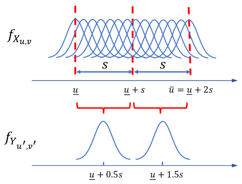
Figure 5: Illustration of the data release mechanism for continuous distributions when secret=mean.

Proposition 1.

Under Assumption 1, Mechanism 1 has privacy $\Pi_{\epsilon,\omega_{\Theta}}{}\leq\frac{2\epsilon}{s}$ and distortion $\Delta=\frac{s}{2}<2\Delta_{\text{opt}}(\Pi_{\epsilon,\omega_{\Theta}}{})$, where $\Delta_{\text{opt}}(\Pi_{\epsilon,\omega_{\Theta}}{})$ is the minimal distortion any data release mechanism can achieve given privacy level $\Pi_{\epsilon,\omega_{\Theta}}{}$.

The proof is in § C-B. The two takeaways from this proposition are that: (1) the data holder can use $s$ to control the trade-off between distortion and privacy, and (2) the mechanism achieves an order-optimal distortion with multiplicative factor $2$.

VI-B Secret = Quantiles

In this section, we show how to protect the $\alpha$-quantile of the exponential distribution and the shifted exponential distribution. We analyze the Gaussian and uniform distributions in Appendix F. We choose these distributions as a starting point of our analysis as many distributions in real-world data can be approximated by one of these distributions.

In our analysis, the parameters of (shifted) exponential distributions are denoted by:

• Exponential distribution: $\theta=\lambda$, where $\lambda$ is the scale parameter: $f_{X_{\lambda}}\left(x\right)=\frac{1}{\lambda}e^{-x/\lambda}$.

• Shifted exponential distribution generalizes the exponential distribution with an additional shift parameter $h$: $\theta=\left(\lambda,h\right)$. In other words, $f_{X_{\lambda,h}}\left(x\right)=\frac{1}{\lambda}e^{-\left(x-h\right)/\lambda}$.

As before, we first present a lower bound.

Corollary 2 (Privacy lower bound, secret = $\alpha$-quantile of a continuous distribution).

Consider the secret function $g\left(\theta\right)=\alpha$-quantile of $f_{X_{\theta}}$. For any $T\in\left(0,1\right)$, when $\Pi_{\epsilon,\omega_{\Theta}}\leq T$, we have $\Delta>\left(\lceil{\frac{1}{T}}\rceil-1\right)\cdot 2\ratio\epsilon$, where is defined as follows:

• Exponential:

  $$\ratio=-\frac{1}{2\ln\left(1-\alpha\right)}.$$

• Shifted exponential:

  $$\ratio=\begin{cases}\frac{1}{2}\left|1+\frac{\ln(1-\alpha)+1}{W_{-1}\left(-\frac{\ln\left(1-\alpha\right)+1}{2\left(1-\alpha\right)e}\right)}\right|&\alpha\in[0,1-e^{-1})\\ \frac{1}{2}\left|1+\frac{\ln(1-\alpha)+1}{W_{0}\left(-\frac{\ln\left(1-\alpha\right)+1}{2\left(1-\alpha\right)e}\right)}\right|&\alpha\in[1-e^{-1},1)\end{cases},$$

  where $W_{-1}$ and $W_{0}$ are Lambert $W$ functions.

The proof is in § C-C. Next, we provide data release mechanisms for each of the distributions that achieve trade-offs close to these bounds.

Mechanism 2 (For secret = $\alpha$-quantile of a continuous distribution).

We design mechanisms for each of the distributions. In both cases, $s>0$ is the quantization bin size chosen by the operator to divide $\left(\overline{\lambda}-\underline{\lambda}\right)$, where $\overline{\lambda}$ and $\underline{\lambda}$ are upper and lower bounds of $\lambda$.

• Exponential:

  $$\mathcal{S}_{i} =\left[\underline{\lambda}+i\cdot s,\underline{\lambda}+\left(i+1\right)\cdot s\right)~{}~{},$$

  $$\theta^{*}_{i} =\underline{\lambda}+\left(i+0.5\right)\cdot s~{}~{},$$

  $$\mathcal{I} =\mathbb{N}.$$

• Shifted exponential:

  $$\mathcal{S}_{i,h} =\left\{\left(\underline{\lambda}+\left(i+0.5\right)s+t,h-t_{0}\cdot t\right)|t\in\left[-\frac{s}{2},\frac{s}{2}\right)\right\}~{}~{},$$

  $$\theta^{*}_{i,h} =\left(\underline{\lambda}+\left(i+0.5\right)s,h\right)~{}~{},$$

  $$\mathcal{I} =\left\{(i,h)|i\in\mathbb{N},h\in\mathbb{R}\right\},$$

  where

  $$t_{0} =\begin{cases}-1-\ln\left(1-\alpha\right)-W_{-1}\left(-\frac{\ln\left(1-\alpha\right)+1}{2\left(1-\alpha\right)e}\right)&\left(\alpha\in[0,1-e^{-1})\right)\\ -1-\ln\left(1-\alpha\right)-W_{0}\left(-\frac{\ln\left(1-\alpha\right)+1}{2\left(1-\alpha\right)e}\right)&\left(\alpha\in[1-e^{-1},1)\right)\end{cases}.$$

For the privacy-distortion trade-off analysis of Mechanism 2, we assume that the parameters of the original data are drawn from a uniform distribution with lower and upper bounds. Again, we relax this assumption to Lipschitz priors in § D-B. Precisely,

Assumption 2.

The prior over distribution parameters is:

• Exponential: follows the uniform distribution over $\left[\underline{\lambda},\overline{\lambda}\right)$.

• Shifted exponential: $\left(\lambda,h\right)$ follows the uniform distribution over $\left\{(a,b)|a\in\left[\underline{\lambda},\overline{\lambda}\right),b\in\left[\underline{h},\overline{h}\right)\right\}$.

We relax Assumption 2 and analyze the privacy-distortion trade-off of Mechanism 2 in § D-B.

Proposition 2.

Under Assumption 2, Mechanism 2 has the following $\Pi_{\epsilon,\omega_{\Theta}}{}$ and $\Delta$ value/bound.

• Exponential:

  $$\Pi_{\epsilon,\omega_{\Theta}}=\frac{2\epsilon}{-\ln\left(1-\alpha\right)s},\quad\quad\Delta=\frac{1}{2}s<2\Delta_{\text{opt}}.$$

• Shifted exponential:

  $$\Pi_{\epsilon,\omega_{\Theta}} <\frac{2\epsilon}{\lvert\ln\left(1-\alpha\right)+t_{0}\rvert s}+\frac{\lvert t_{0}\rvert s}{\overline{h}-\underline{h}},$$

  $$\Delta =\frac{s}{2}\left(t_{0}-1\right)+se^{-t_{0}}<\left(2+\frac{\lvert t_{0}\rvert\cdot\lvert\ln\left(1-\alpha\right)+t_{0}\rvert s^{2}}{\epsilon\left(\overline{h}-\underline{h}\right)}\right)\Delta_{\text{opt}}.$$

  Under the high-precision regime where ${\frac{s^{2}}{\overline{h}-\underline{h}}}\rightarrow 0$ as $s,(\overline{h}-\underline{h})\to\infty$, when $\alpha\in[0.01,0.25]\cup[0.75,0.99]$, $\Delta$ satisfies

  $$\lim\sup_{{\frac{s^{2}}{\overline{h}-\underline{h}}}\rightarrow 0}\Delta<3\Delta_{\text{opt}}.$$

$\Delta_{\text{opt}}$ is the optimal achievable distortion given the privacy achieved by Mechanism 2, and $t_{0}$ is a constant defined in Mechanism 2.

The proof is in § C-D. Note that the quantization bin size $s$ cannot be too small, or the attacker can always successfully guess the secret within a tolerance $\epsilon$ (i.e., $\Pi_{\epsilon,\omega_{\Theta}}{}=1$). Therefore, for the “high-precision” regime, we consider the asymptotic scaling as both $s$ and $\overline{h}-\underline{h}$ grow. When $s>1$, the scaling condition ${\frac{s^{2}}{\overline{h}-\underline{h}}}\rightarrow 0$ implies a more interpretable condition of ${\frac{s}{\overline{h}-\underline{h}}}\rightarrow 0$, which says that the bin size is small relative to the parameter space. For example, this condition is required when the secret tolerance $\epsilon>1/2$ (i.e., we need a bin size $s>1$ to achieve non-trivial privacy guarantees).

Proposition 2 shows that the quantization mechanism is order-optimal with multiplicative factor $2$ for the exponential distribution. For shifted exponential distribution, order-optimality holds asymptotically in the high-precision regime.

VI-C Extending Data Release Mechanisms for Dataset Input/Output

The data release mechanisms discussed in previous sections assume that data holders know the distribution parameter of the original data. In practice, data holders often only have a dataset of samples from the data distribution and do not know the parameters of the underlying distributions. The quantization data release mechanisms can be easily adapted to handle dataset input/output.

The high-level idea is that the data holders can estimate the distribution parameters $\theta$ from the data samples and find the corresponding quantization bins $\mathcal{S}_{i}$ according to the estimated parameters, and then modify the original samples as if they are sampled according to the released parameter $\theta^{*}_{i}$. This may be infeasible for high-dimensional parameter vectors $\theta$; we did not explore this question in the current work. For brevity, we only present the concrete procedure for secret=mean on continuous distributions as an example. For a dataset of $\mathcal{X}=\left\{x_{1},\ldots,x_{n}\right\}$, the procedure is:

1. Estimate the mean from the data samples: $\hat{\mu}=\frac{1}{n}\sum_{i\in[n]}x_{i}$.

2. According to Eq. 13, compute the index of the corresponding set $i=\lfloor{\frac{\hat{\mu}-\underline{\mu}}{s}}\rfloor$.

3. According to Eq. 14, change the mean of the data samples to $\mu_{target}=\underline{\mu}+\left(i+0.5\right)\cdot s$. This can be done by sample-wise operation $x_{i}^{\prime}=x_{i}-\hat{\mu}+\mu_{target}$.

4. The released dataset is $\mathcal{M}_{g}\left(\mathcal{X},z\right)=\left\{x_{1}^{\prime},\ldots,x_{n}^{\prime}\right\}$.

Note that this mechanism applies to samples. Therefore, it can be applied either to the original data, or as an add-on to existing data sharing tools [45, 15, 46, 47, 48]. For example, it can be used to modify synthetically-generated samples after they are generated, or to modify the training dataset for a generative model, or to directly modify the original data for releasing.

VII Experiments

In the previous sections, we theoretically demonstrated the privacy-distortion tradeoffs of our data release mechanisms in some special case studies. In this section, we focus on orthogonal questions through real-world experiments: (1) how well our data release mechanisms perform in practice when the assumptions do not hold, and (2) how summary statistic privacy quantitatively compares with existing privacy frameworks (which we explained qualitatively in § II). The code is open-sourced at https://github.com/fjxmlzn/summary_statistic_privacy.

Datasets.  We use two real-world datasets to simulate the motivating scenarios.

1. Wikipedia Web Traffic Dataset (WWT) [49] contains the daily page views of 145,063 Wikipedia web pages in 2015-2016. To preprocess it for our experiments, we remove the web pages with empty page view record on any day (117,277 left), and compute the mean page views across all dates for each web page. Our goal is to release the page views (i.e., a 117,277-dimensional vector) while protecting the mean of the distribution (which reveals the business scales of the company).

2. Measuring Broadband America Dataset (MBA) [50] contains network statistics (including network traffic counters) collected by United States Federal Communications Commission from homes across United States. We select the average network traffic (GB/measurement) from AT&T clients as our data. Our goal is to release a copy of this data while hiding the 0.95-quantile (which reveals the network capability).

Baselines.  We compare our mechanisms discussed in § VI with three popular mechanisms proposed in prior work (§ II): differentially-private density estimation [23] (shortened to DP), attribute-private Gaussian mechanism [18] (shortened to AP), and Wasserstein mechanism for distribution privacy [27] (shortened to DistP). As these mechanisms provide different privacy guarantees than summary statistic privacy, it is difficult to do a fair comparison between these baselines and our quantization mechanism. We include them to quantitatively show the differences (and similarities) between various privacy frameworks.

For a dataset of samples $\mathcal{X}=\left\{x_{1},...,x_{n}\right\}$, DP works by: (1) Dividing the space into $m$ bins: $B_{1},...,B_{m}$.(2) Computing the histogram $C_{i}=\sum_{j=1}^{n}\mathbb{I}\left(x_{j}\in B_{i}\right)$. (3) Adding noise to the histograms $D_{i}=\max\left\{0,C_{i}+\text{Laplace}\left(0,\beta^{2}\right)\right\}$, where $\text{Laplace}\left(0,\beta^{2}\right)$ means a random noise from Laplace distribution with mean 0 and variance $\beta^{2}$. (4) Normalizing the histogram $p_{i}=\frac{D_{i}}{\sum_{j=1}^{m}D_{j}}$. We can then draw $y_{i}$ according to the histogram and release $\mathcal{Y}=\left\{y_{1},...,y_{n}\right\}$ with differential privacy guarantees. AP works by releasing $\mathcal{Y}=\left\{x_{i}+\mathcal{N}\left(0,\beta^{2}\right)\right\}_{i=1}^{n}$.DistP works by releasing $\mathcal{Y}=\left\{x_{i}+\text{Laplace}\left(0,\beta^{2}\right)\right\}_{i=1}^{n}$. Note that for each of these mechanisms, normally their noise parameters would be set carefully to match the desired privacy guarantees (e.g., differential privacy). In our case, since our privacy metric is different, it is unclear how to set the noise parameters for a fair privacy comparison. For this reason, we evaluate different settings of the noise parameters, and measure the empirical tradeoffs.

Metrics.  Our privacy and distortion metrics depend on the prior distribution of the original data $\theta\sim\omega_{\Theta}$ (though the mechanism does not). In practice (and also in these experiments), the data holder only has one dataset. Therefore, we cannot empirically evaluate the proposed privacy and distortion metrics, and resort to surrogate metrics to bound our true privacy and distortion.

Surrogate privacy metric.  For an original dataset $\mathcal{X}=\left\{x_{1},...,x_{n}\right\}$ and the released dataset $\mathcal{Y}=\left\{y_{1},...,y_{n}\right\}$, we define the surrogate privacy metric $\tilde{\Pi}_{\epsilon}$ as the error of an attacker who guesses the secret of the released dataset as the true secret: $\tilde{\Pi}_{\epsilon}\triangleq-\left|g\left(\mathcal{X}\right)-g\left(\mathcal{Y}\right)\right|$, where $g\left(\mathcal{D}\right)=$ mean of $\mathcal{D}$ and $0.95$-quantile of $\mathcal{D}$ in WWT and MBA datasets respectively. Note that in the definition of $\tilde{\Pi}_{\epsilon}$, a minus sign is added so that a smaller value indicates stronger privacy, as in privacy metric Eq. 2. This simple attacker strategy is in fact a good proxy for evaluating the privacy $\Pi_{\epsilon,\omega_{\Theta}}$ due to the following facts. (1) For our data release mechanisms for these secrets Mechanisms 1, 2 and 5, when the prior distribution is uniform, this strategy is actually optimal, so there is a direct mapping between $\tilde{\Pi}_{\epsilon}$ and $\Pi_{\epsilon,\omega_{\Theta}}$. (2) For AP applied on protecting mean of the data (i.e., Wikipedia Web Traffic Dataset experiments), this strategy gives an unbiased estimator of the secret. (3) For DP and AP on other cases, this mechanism may not be an unbiased estimator of the secret, but it gives an upper bound on the attacker’s error.

Surrogate distortion metric.  We define our surrogate distortion metric as the Wasserstein-1 distance between the two datasets: $\tilde{\Delta}\triangleq d\left(p_{\mathcal{X}}\|p_{\mathcal{Y}}\right)$ where $p_{D}$ denotes the empirical distribution of a dataset $D$. This metric evaluates how much the mechanism distorts the dataset.

In fact, we can deduce a theoretical lower bound for the surrogate privacy and distortion metrics for secret = mean (shown later in Fig. 6) using similar techniques as the proofs in the main paper (see § C-E).

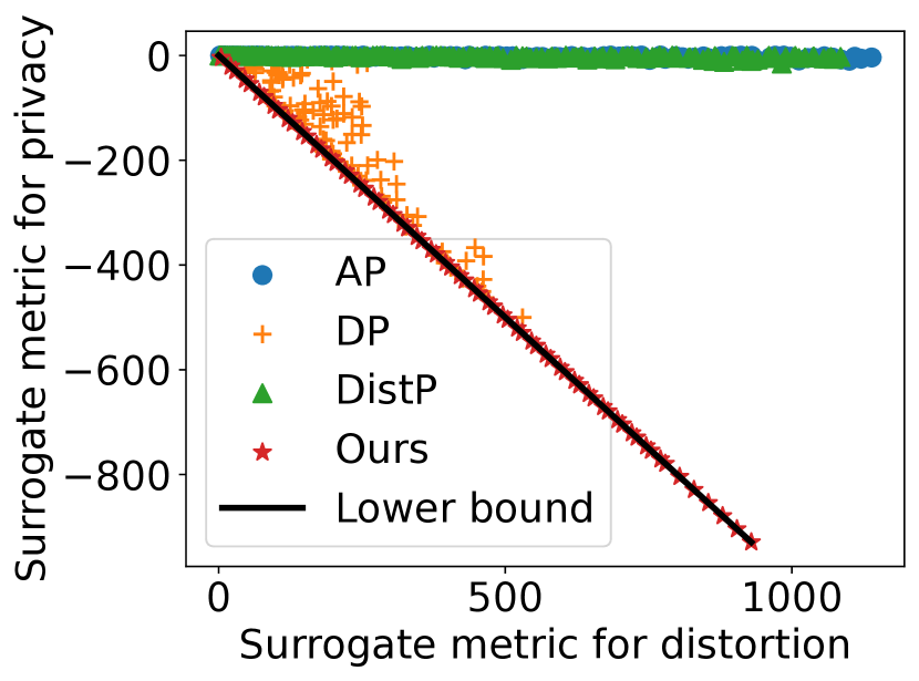
(a) Wikipedia Web Traffic Dataset.
(secret=mean)

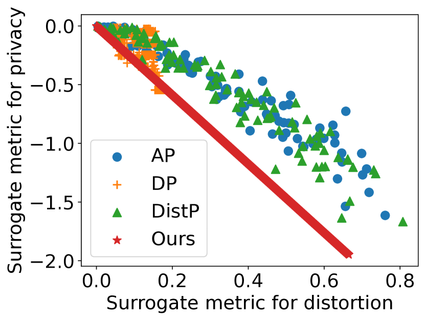
(b) Measuring Broadband America Dataset.
(secret=quantile)

Figure 6: Privacy (lower is better) and distortion (lower is better) of AP, DP, DistP, and ours. Each point represents one instance of data release mechanism with one hyper-parameter. “Lower bound” is the theoretical lower bound of the achievable region. Our data release mechanisms achieve better privacy-distortion tradeoff than AP, DP, and DistP.

VII-A Results

We enumerate the hyper-parameters of each method (bin size and $\beta$ for DP, $\beta$ for AP and DistP, and $s$ for ours). For each method and each hyper-parameter, we compute their surrogate privacy and distortion metrics. The results are shown in Fig. 6 (bottom left is best); each data point represents one realization of mechanism $\mathcal{M}_{g}$ under a distinct hyperparameter setting. Two takeaways are below.

(1) The proposed quantization data release mechanisms has a good surrogate privacy-distortion trade-off, even when the assumptions do not hold. In practical scenarios, the data distributions analyzed in § VI and in the Appendices may not always match real data exactly. Our data release mechanism for mean (i.e., Mechanism 1 used in WWT) supports general continuous distributions, and therefore, there is no such a distribution gap. Indeed, even for these surrogate metrics, our Mechanism 1 is also optimal (see § C-E). This is visualized in Fig. 6(a) where we can see that our data release mechanism matches the theoretical lower bound of the trade-off. However, the quantization data release mechanisms for quantiles (i.e., Mechanism 2 used in Fig. 6(b)) are order-optimal only when the distributions are within certain classes (§ VI-B). Observing that network traffic in MBA follows a one-side fat-tailed distribution (not shown), we apply the data release mechanism for the exponential distribution (Mechanism 2) for this dataset (which is not heavy-tailed). Despite the distribution mismatch, the quantization data release mechanism still achieves a good privacy-distortion compared to DP, AP, and DistP (Fig. 6(b)). More discussions are below.

(2) The quantization data release mechanisms achieve better privacy-distortion trade-off than DP, AP, and DistP. AP and DistP directly add Gaussian/Laplace noise to each sample. This process does not change the mean of the distribution on expectation. Therefore, Figure 6 shows that AP and DistP have a bad privacy-distortion tradeoff. DP quantizes (bins) the samples before adding noise. Quantization has a better property in terms of protecting the mean of the distribution, and therefore we see that DP has a better privacy-distortion tradeoff than AP and DistP, but still worse than the quantization mechanism. Note that in Fig. 6(b), a few of the DP instances have better privacy-distortion trade-offs than ours. This is not an indication that DP is fundamentally better. Due to the randomness in DP (from the added Laplace noise), some realizations of the noise in this experiment happened to lead to a better trade-off. Another instance of the DP algorithm could lead to a bad trade-off, and therefore, DP’s achievable trade-off points are widespread.

In summary, these empirical results confirm the intuition in § II that DP, AP, and DistP may not achieve good privacy-utility tradeoffs for our problem. This is expected—they are designed for a different objective. Additional results on downstream tasks are in Appendix I.

VIII Discussion and Future Work

This work introduces a framework for summary statistic privacy concerns in data sharing applications. This framework can be used to analyze the leakage of statistical information and the privacy-distortion trade-offs of data release mechanisms (§ III and IV). The quantization data release mechanisms can be used to protect statistical information (§ V and VI). However, many interesting open questions for future work remain.

Composition guarantees.  A limitation of the current privacy metric $\Pi_{\epsilon,\omega_{\Theta}}$ is that it does not provide composition guarantees; in other words, if one applies a summary statistic-private mechanism $\upsilon$ times, we cannot easily bound the privacy parameter of the $\upsilon$-fold composed mechanism. In contrast, composition is an important and desirable property exhibited by differential privacy [16]. The lack of composition can be problematic in situations where a data holder wants to release a dataset (or correlated datasets) multiple times. Understanding how to alter the definition to provide composition may be useful.

Number of secrets.  In this work, we studied the case where the data holder only wishes to hide a single secret. In practice, data holders often want to hide multiple properties of their underlying data. It would be useful to understand how to best extend the analysis to such a setting.

The dimension and the type of data distributions.  Although the proof for the lower bound in Section IV applies to general prior distributions, we analyze the quantization mechanism under a limited set of one-dimensional distributions (Table I), assuming different parameters of the distribution are drawn independently of each other. An interesting direction for future work is to define mechanisms that have good tradeoffs under prior distributions with correlated parameters and priors.

Relation to Differential Privacy  Figure 6 suggests that despite being designed for a different threat model, the DP mechanism does fairly well. As mentioned, this is because the mchanism first bins data points, which is similar to quantization. However, this raises an important question: under what conditions on the true data, the secret quantity, and the mechanism do differentially-private mechanisms achieve a good privacy-utility tradeoff for our problem?

Approximation error.  We studied a number of data distributions and prior distributions in this work. However, an interesting question is to bound the error in privacy and distortion metrics as a function of approximation error when describing either the original data distribution or the prior.

Extensions.  Finally, one limitation of the current privacy metric $\Pi_{\epsilon,\omega_{\Theta}}$ is that it depends on the prior distribution of the parameters $\omega_{\Theta}$, which is unknown in many applications. Motivated by maximal leakage [20], one possibility is to consider a normalized privacy metric:

$$\Pi_{\epsilon,\omega_{\Theta}}^{\prime}\triangleq\sup_{\omega_{\Theta}}~{}\log\frac{\Pi_{\epsilon,\omega_{\Theta}}}{\sup_{\hat{g}}~{}\mathbb{P}\left(\hat{g}\left(\omega_{\Theta}\right)\in\left[g\left(\theta\right)-\epsilon,g\left(\theta\right)+\epsilon\right]\right)},$$

where $\hat{g}\left(\omega_{\Theta}\right)$ is an attacker that knows the prior distribution but does not see the released data, and the denominator is the probability that the strongest attacker guesses the secret within tolerance $\epsilon$. Similar to maximal leakage, we consider the worst-case leakage among all possible priors. This normalized $\Pi_{\epsilon,\omega_{\Theta}}^{\prime}$ considers how much additional “information” that the released data provides to the attacker in the worst-case (see also inferential privacy [51]).

Appendix A Analysis of the Alternative Formulation

In this section, we present the alternative formulation of minimizing privacy metric $\Pi_{\epsilon,\omega_{\Theta}}{}$ subject to a constraint on distortion $\Delta{}$:

$$\begin{split}\min_{\mathcal{M}_{g}}~{}~{}\Pi_{\epsilon,\omega_{\Theta}}{}\quad\quad\quad\text{subject to}~{}~{}\Delta\leq T\end{split}$$ (16)

Theorem 2 (Lower bound of privacy-distortion tradeoff).

Let $D\left(X_{\theta_{1}},X_{\theta_{2}}\right)\triangleq\frac{1}{2}d\left(\omega_{X_{\theta_{1}}}\|\omega_{X_{\theta_{2}}}\right)$, where $d\left(\cdot\|\cdot\right)$ is defined in Eq. 3. Further, let $R\left(X_{\theta_{1}},X_{\theta_{2}}\right)\triangleq\lvert g{({{\theta_{1}}})-g{({{\theta_{2}}})}}\rvert$, and let $\ratio\triangleq$ $\ \inf_{\theta_{1},\theta_{2}\in\text{Supp}\left(\omega_{\Theta}\right)}\frac{D\left(X_{\theta_{1}},X_{\theta_{2}}\right)}{R\left(X_{\theta_{1}},X_{\theta_{2}}\right)}$. For any $T>0$, when $\Delta\leq T$, we have $\Pi_{\epsilon,\omega_{\Theta}}\geq\lceil{\frac{T}{2\ratio\epsilon}}\rceil^{-1}$.

Proof.

For any $\theta^{\prime}$, we have

$$T \geq\Delta$$

$$\geq\sup_{\theta\in\text{Supp}\left(\omega_{\Theta}\right),z\in\text{Supp}\left(\omega_{Z}\right):\mathcal{M}_{g}\left(\theta,z\right)=\theta^{\prime}}d\left(\omega_{X_{\theta}}\|\omega_{X_{\theta^{\prime}}}\right)$$

$$\geq\sup_{\theta_{i}\in\text{Supp}\left(\omega_{\Theta}\right),z_{i}:\mathcal{M}_{g}\left(\theta_{i},z_{i}\right)=\theta^{\prime}}D\left(X_{\theta_{1}},X_{\theta_{2}}\right)$$ (17)

$$\geq\ratio\cdot\sup_{\theta_{i}\in\text{Supp}\left(\omega_{\Theta}\right),z_{i}:\mathcal{M}_{g}\left(\theta_{i},z_{i}\right)=\theta^{\prime}}R\left(X_{\theta_{1}},X_{\theta_{2}}\right)$$

where Eq. 17 comes from triangle inequality.

Let

$$L_{\theta^{\prime}}\triangleq\inf_{\theta\in\text{Supp}\left(\omega_{\Theta}\right),z:\mathcal{M}_{g}\left(\theta,z\right)=\theta^{\prime}}g\left(\theta\right)~{},$$

$$R_{\theta^{\prime}}\triangleq\sup_{\theta\in\text{Supp}\left(\omega_{\Theta}\right),z:\mathcal{M}_{g}\left(\theta,z\right)=\theta^{\prime}}g\left(\theta\right)~{}.$$

From the above result, we know that $R_{\theta^{\prime}}-L_{\theta^{\prime}}\leq\frac{T}{\ratio}$. We can define a sequence of attackers such that $\hat{g}_{i}\left(\theta^{\prime}\right)=L_{\theta^{\prime}}+\left(i+0.5\right)\cdot 2\epsilon$ for $i\in\left\{0,1,\ldots,\lceil{\frac{T}{2\ratio\epsilon}}\rceil-1\right\}$ (Fig. 7).

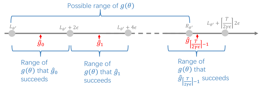
Figure 7: The construction of attackers for proof of Theorem 2. The $2\epsilon$ ranges of $\hat{g}_{0},...,\hat{g}_{\lceil{\frac{T}{2\ratio\epsilon}}\rceil-1}$ jointly cover the entire range of possible secret $\left[L_{\theta^{\prime}},R_{\theta^{\prime}}\right]$. Therefore, there exists one attacker whose probability of guessing the secret correctly within $\epsilon$ is $\geq\lceil{\frac{T}{2\ratio\epsilon}}\rceil^{-1}$ (Eq. 18).

We have

$$\sum_{i}\mathbb{P}\left(\hat{g}_{i}\left(\theta^{\prime}\right)\in\left[g\left(\theta\right)-\epsilon,g\left(\theta\right)+\epsilon\right]\bigg{|}\theta^{\prime}\right)\geq 1,$$

and therefore,

$$\max_{i}\mathbb{P}\left(\hat{g}_{i}\left(\theta^{\prime}\right)\in\left[g\left(\theta\right)-\epsilon,g\left(\theta\right)+\epsilon\right]\bigg{|}\theta^{\prime}\right)\geq\lceil{\frac{T}{2\ratio\epsilon}}\rceil^{-1},$$ (18)

which implies that

$$\sup_{\hat{g}}\mathbb{P}\left(\hat{g}\left(\theta^{\prime}\right)\in\left[g\left(\theta\right)-\epsilon,g\left(\theta\right)+\epsilon\right]\bigg{|}\theta^{\prime}\right)\geq\lceil{\frac{T}{2\ratio\epsilon}}\rceil^{-1}.$$

Therefore, we have

$$\Pi_{\epsilon,\omega_{\Theta}}{} =\sup_{\hat{g}}\mathbb{P}\left(\hat{g}\left(\theta^{\prime}\right)\in\left[g\left(\theta\right)-\epsilon,g\left(\theta\right)+\epsilon\right]\right)$$

$$=\sup_{\hat{g}}\mathbb{E}\left(\mathbb{P}\left(\hat{g}\left(\theta^{\prime}\right)\in\left[g\left(\theta\right)-\epsilon,g\left(\theta\right)+\epsilon\right]\bigg{|}\theta^{\prime}\right)\right)$$

$$=\mathbb{E}\left(\sup_{\hat{g}}\mathbb{P}\left(\hat{g}\left(\theta^{\prime}\right)\in\left[g\left(\theta\right)-\epsilon,g\left(\theta\right)+\epsilon\right]\bigg{|}\theta^{\prime}\right)\right)$$

$$\geq\lceil{\frac{T}{2\ratio\epsilon}}\rceil^{-1}.$$

∎

Appendix B Binary Search and Greedy Algorithms for Designing Quantization Mechanism

We use the binary search algorithm in Algorithm 2 to search for the distortion budget that matches the privacy budget under the optimal data release mechanism.

Input : Parameter range: $\left[\underline{\theta},\overline{\theta}\right)$

Privacy budget: $T$

Distortion budget search range: $[\underline{B},\overline{B}]$

Step size: $s$ (which divides $\overline{\theta}-\underline{\theta}$)

Precision: $\eta$

1

2while $\overline{T}-\underline{T}\geq\eta$ do

3       $pri,\mathcal{S},\theta^{\prime}\leftarrow\text{Algorithm-1}\left(\left[\underline{\theta},\overline{\theta}\right),\frac{\overline{T}+\underline{T}}{2},\kappa\right)$

4      

5      if $pri>T$ then

6            $\underline{B}\leftarrow\frac{\overline{T}+\underline{T}}{2}$

7      else

8            $\overline{B}\leftarrow\frac{\overline{T}+\underline{T}}{2}$

9      

10

return Data release mechanism parameters: $\mathcal{S},\theta^{\prime}$

Algorithm 2 Data release mechanism with privacy budget.

We provide the greedy algorithm in Algorithm 3. In this algorithm, we greedily select the ranges of $\theta$ for each $\mathcal{S}_{i}$ in order. The left end point of the first range is the parameter lower bound (Algorithm 3). We then scan across all possible right end point such that the distortion for this range will not exceed the budget $T$ (Algorithm 3), and pick the one that gives the minimal attacker confidence (Algorithm 3). After deciding the range of $\theta$, we will set of the released distribution for this range (Algorithm 3), and then move on to the next range (Algorithm 3). The time complexity of this algorithm is $\mathcal{O}\left(\left(\nicefrac{{\overline{\theta}-\underline{\theta}}}{{\kappa}}\right)^{2}\cdot\mathcal{C}_{D}\cdot\mathcal{C}_{P}\right)$, the same as the dynamic programming algorithm.

Input : Parameter range: $\left(\underline{\theta},\overline{\theta}\right]$

Prior over parameter: $f_{\Theta}$

Distortion budget: $T$

Step size: $\kappa$ (which divides $\overline{\theta}-\underline{\theta}$)

1 $\mathcal{I}\leftarrow\emptyset$

2 $L\leftarrow\underline{\theta}$

3 $privacy\leftarrow 0$

4 while $L<\overline{\theta}$ do

5       $min\_p\leftarrow\infty$

6       $min\_R\leftarrow$ NULL

7       $R\leftarrow L$

8       while $R\leq\overline{\theta}$ and $\mathcal{D}\left(L,R\right)\leq T$ do

9             $p\leftarrow\mathcal{P}\left(L,R\right)$

10             if $p\leq min\_p$ then

11                   $min\_p\leftarrow p$

12                   $min\_R\leftarrow R$

13                  

14            $R\leftarrow R+\kappa$

15            

16      if $min\_R$ is not NULL then

17             $\mathcal{S}_{L}\leftarrow\left\{X_{\theta}:\theta\in\left(L,~{}min\_R\right]\right\}$

18             $\theta^{\prime}_{L}\leftarrow\mathcal{D}\left(L,min\_R\right)$

19             $\mathcal{I}\leftarrow\mathcal{I}\cup\left\{L\right\}$

20             $privacy\leftarrow\frac{\int_{\underline{\theta}}^{L}f_{\Theta}\left(t\right)\mathrm{d}t}{\int_{\underline{\theta}}^{min\_R}f_{\Theta}\left(t\right)\mathrm{d}t}\cdot privacy+\frac{\int_{L}^{min\_R}f_{\Theta}\left(t\right)\mathrm{d}t}{\int_{\underline{\theta}}^{min\_R}f_{\Theta}\left(t\right)\mathrm{d}t}\cdot min\_p$

21      else

22            ERROR: No answer

23      $L\leftarrow min\_R$

return $privacy$, $\left\{\mathcal{S}_{i}:i\in\mathcal{I}\right\},\left\{\theta^{\prime}_{i}:i\in\mathcal{I}\right\}$

Algorithm 3 Greedy-based data release mechanism for single-parameter distributions.

Appendix C Proofs

C-A Proof of Corollary 1

Proof.

For any $X_{\theta_{1}},X_{\theta_{2}}$, we have

$$D\left(X_{\theta_{1}},X_{\theta_{2}}\right) =\frac{1}{2}d_{\text{Wasserstein-1}}\left(\omega_{X_{\theta_{1}}}\|\omega_{X_{\theta_{2}}}\right)$$

$$\geq\frac{1}{2}\lvert g\left(\theta_{1}\right)-g\left(\theta_{2}\right)\rvert$$ (19)

$$=\frac{1}{2}R\left(X_{\theta_{1}},X_{\theta_{2}}\right).$$

where Eq. 19 comes from Jensen’s inequality. Therefore, we have $\ratio=\inf_{\theta_{1},\theta_{2}\in\text{Supp}\left(\omega_{\Theta}\right)}\frac{D\left(X_{\theta_{1}},X_{\theta_{2}}\right)}{R\left(X_{\theta_{1}},X_{\theta_{2}}\right)}\geq\frac{1}{2}$. The result then follows from Theorem 1. ∎

C-B Proof of Proposition 1

Proof.

For any released parameter $\theta^{\prime}=(u^{\prime},v^{\prime})$, there exists $i\in\left\{0,...,N-1\right\}$ such that $u^{\prime}=\underline{u}+\left(i+0.5\right)\cdot s$. We have

$$\sup_{\hat{g}} \mathbb{P}\left(\hat{g}\left(\theta^{\prime}\right)\in\left[g\left(\theta\right)-\epsilon,g\left(\theta\right)+\epsilon\right]\big{|}\theta^{\prime}\right)$$

$$=\sup_{\hat{g}}\int_{\underline{u}+i\cdot s}^{\underline{u}+\left(i+1\right)\cdot s}f_{U|U^{\prime}}\left(u|u^{\prime}\right)\cdot\int_{u-\epsilon}^{u+\epsilon}f_{\hat{g}\left(u^{\prime},v^{\prime}\right)}\left(h\right)\ \mathrm{d}h\ \mathrm{d}u$$

$$=\sup_{\hat{g}}\int_{\underline{u}+i\cdot s-\epsilon}^{\underline{u}+\left(i+1\right)\cdot s+\epsilon}f_{\hat{g}\left(u^{\prime},v^{\prime}\right)}(h)\cdot\int_{\hat{g}\left(f_{X_{u^{\prime},v^{\prime}}}\right)-\epsilon}^{\hat{g}\left(f_{X_{u^{\prime},v^{\prime}}}\right)+\epsilon}f_{U|U^{\prime}}\left(u|u^{\prime}\right)\ \mathrm{d}u\ \mathrm{d}h$$

$$\leq\sup_{\hat{g}}\int_{\underline{u}+i\cdot s-\epsilon}^{\underline{u}+\left(i+1\right)\cdot s+\epsilon}\frac{2\epsilon}{s}\cdot f_{\hat{g}\left(u^{\prime},v^{\prime}\right)}(h)\ \mathrm{d}h$$

$$\leq\frac{2\epsilon}{s}.$$

Therefore, we have

$$\Pi_{\epsilon,\omega_{\Theta}}{} =\sup_{\hat{g}}\mathbb{P}\left(\hat{g}\left(\theta^{\prime}\right)\in\left[g\left(\theta\right)-\epsilon,g\left(\theta\right)+\epsilon\right]\right)$$

$$=\sup_{\hat{g}}\mathbb{E}\left(\mathbb{P}\left(\hat{g}\left(\theta^{\prime}\right)\in\left[g\left(\theta\right)-\epsilon,g\left(\theta\right)+\epsilon\right]\bigg{|}\theta^{\prime}\right)\right)$$

$$=\mathbb{E}\left(\sup_{\hat{g}}\mathbb{P}\left(\hat{g}\left(\theta^{\prime}\right)\in\left[g\left(\theta\right)-\epsilon,g\left(\theta\right)+\epsilon\right]\bigg{|}\theta^{\prime}\right)\right)$$

$$\leq\frac{2\epsilon}{s}.$$

For the distortion, we can easily get that $\Delta=\frac{s}{2}$. According to Corollary 1, we have $\Delta_{\text{opt}}>\left(\lceil{\frac{1}{\Pi_{\epsilon,\omega_{\Theta}}{}}}\rceil-1\right)\epsilon\geq\epsilon$. We can get that

$$\Delta =\Delta_{\text{opt}}+\Delta-\Delta_{\text{opt}}$$

$$<\Delta_{\text{opt}}+\Delta-\left(\lceil{\frac{1}{\Pi_{\epsilon,\omega_{\Theta}}}}\rceil-1\right)\cdot\epsilon$$

$$\leq\Delta_{\text{opt}}+\epsilon+\Delta-{{\frac{\epsilon}{\Pi_{\epsilon,\omega_{\Theta}}}}}$$

$$\leq\Delta_{\text{opt}}+\epsilon$$

$$\leq 2\Delta_{\text{opt}}.$$

∎

C-C Proof of Corollary 2

C-C1 Exponential Distribution

Proof.

Let $X_{\lambda_{1}},X_{\lambda_{2}}$ be two exponential random variables. We have

$$\frac{D\left(X_{\lambda_{1}},X_{\lambda_{2}}\right)}{R\left(X_{\lambda_{1}},X_{\lambda_{2}}\right)} =\frac{\frac{1}{2}\left({\lambda_{1}}-{\lambda_{2}}\right)}{-\ln\left(1-\alpha\right)\left({\lambda_{1}}-{\lambda_{2}}\right)}=-\frac{1}{2\ln\left(1-\alpha\right)}.$$ (20)

Therefore we can get that

$$\ratio=-\frac{1}{2\ln\left(1-\alpha\right)}.$$

∎

C-C2 Shifted Exponential Distribution

Proof.

Let $X_{\lambda_{1},h_{1}},X_{\lambda_{2},h_{2}}$ be random variables from shifted exponential distributions. Let $\lambda_{2}\leq\lambda_{1}$ without loss of generality. Let $a=\frac{\lambda_{1}}{\lambda_{2}}$ and $b=\left(h_{1}/\lambda_{1}-h_{2}/\lambda_{2}\right){\lambda_{2}}$. We can get that $f_{X_{\lambda_{1},h_{1}}}\left(x\right)=af_{X_{\lambda_{2},h_{2}}}\left(a\left(x+b\right)\right)$, and

$$D\left(X_{\lambda_{1},h_{1}},X_{\lambda_{2},h_{2}}\right)=\frac{1}{2}d_{\text{Wasserstein-1}}\left(\omega_{X_{\lambda_{1},h_{1}}}\|\omega_{X_{\lambda_{2},h_{2}}}\right)$$

$$=\frac{1}{2}\int_{h_{1}}^{+\infty}\left|x-\left(\frac{x}{a}-b\right)\right|f_{X_{\lambda_{1},h_{1}}}\left(x\right)\mathrm{d}x$$

$$=\frac{\lambda_{2}}{2\lambda_{1}}\int_{h_{1}}^{+\infty}\left|\left(1/\lambda_{2}-1/\lambda_{1}\right)x+h_{1}/\lambda_{1}-h_{2}/\lambda_{2}\right|e^{-\frac{1}{\lambda_{1}}\left(x-h_{1}\right)}\mathrm{d}x$$

$$=\begin{cases}\frac{1}{2}\left(h_{2}-h_{1}+{\lambda_{2}}-{\lambda_{1}}\right)-e^{\frac{h_{2}-h_{1}}{{\lambda_{2}}-{\lambda_{1}}}}\left({\lambda_{2}}-{\lambda_{1}}\right)&\left(h_{1}<h_{2}\right)\\ \frac{1}{2}\left(h_{1}-h_{2}+{\lambda_{1}}-{\lambda_{2}}\right)&\left(h_{1}\geq h_{2}\right)\end{cases},$$ (21)

$$R\left(X_{\lambda_{1},h_{1}},X_{\lambda_{2},h_{2}}\right)=\left|\ln\left(1-\alpha\right)\left({\lambda_{1}}-{\lambda_{2}}\right)+h_{2}-h_{1}\right|.$$

When $h_{1}<h_{2}$, let $t=\frac{h_{2}-h_{1}}{{\lambda_{1}}-{\lambda_{2}}}\in(0,+\infty)$. We have

$$\quad\frac{D\left(X_{\lambda_{1},h_{1}},X_{\lambda_{2},h_{2}}\right)}{R\left(X_{\lambda_{1},h_{1}},X_{\lambda_{2},h_{2}}\right)}$$

$$=\frac{h_{2}-h_{1}+{\lambda_{2}}-{\lambda_{1}}-2e^{\frac{h_{2}-h_{1}}{{\lambda_{2}}-{\lambda_{1}}}}\left({\lambda_{2}}-{\lambda_{1}}\right)}{2\left|\ln\left(1-\alpha\right)\left({\lambda_{1}}-{\lambda_{2}}\right)+h_{2}-h_{1}\right|}$$

$$=\frac{t+2e^{-t}-1}{2\left|\ln\left(1-\alpha\right)+t\right|}$$

$$\geq\begin{cases}\frac{1}{2}\left|1+\frac{\ln(1-\alpha)+1}{W_{-1}\left(-\frac{\ln\left(1-\alpha\right)+1}{2\left(1-\alpha\right)e}\right)}\right|&\alpha\in[0,1-e^{-1})\\ \frac{1}{2}\left|1+\frac{\ln(1-\alpha)+1}{W_{0}\left(-\frac{\ln\left(1-\alpha\right)+1}{2\left(1-\alpha\right)e}\right)}\right|&\alpha\in[1-e^{-1},1)\end{cases},$$

where $W_{-1}$ and $W_{0}$ are Lambert $W$ functions. “$=$” achieves when

$$t=t_{0}\triangleq\begin{cases}-1-\ln\left(1-\alpha\right)-W_{-1}\left(-\frac{\ln\left(1-\alpha\right)+1}{2\left(1-\alpha\right)e}\right)&\left(\alpha\in[0,1-e^{-1})\right)\\ -1-\ln\left(1-\alpha\right)-W_{0}\left(-\frac{\ln\left(1-\alpha\right)+1}{2\left(1-\alpha\right)e}\right)&\left(\alpha\in[1-e^{-1},1)\right)\end{cases}.$$

When $h_{1}\geq h_{2}$, let $t=\frac{h_{1}-h_{2}}{{\lambda_{1}}-{\lambda_{2}}}\in(0,+\infty)$. We have

$$\frac{D\left(X_{\lambda_{1},h_{1}},X_{\lambda_{2},h_{2}}\right)}{R\left(X_{\lambda_{1},h_{1}},X_{\lambda_{2},h_{2}}\right)} =\frac{h_{1}-h_{2}+{\lambda_{1}}-{\lambda_{2}}}{2\left|\ln\left(1-\alpha\right)\left({\lambda_{1}}-{\lambda_{2}}\right)+h_{2}-h_{1}\right|}$$

$$=\frac{t+1}{2\left|\ln\left(1-\alpha\right)-t\right|}$$

$$\geq\min\left\{\frac{1}{2},-\frac{1}{2\ln\left(1-\alpha\right)}\right\}.$$

Therefore we can get that

$$\ratio=\begin{cases}\frac{1}{2}\left|1+\frac{\ln(1-\alpha)+1}{W_{-1}\left(-\frac{\ln\left(1-\alpha\right)+1}{2\left(1-\alpha\right)e}\right)}\right|&\alpha\in[0,1-e^{-1})\\ \frac{1}{2}\left|1+\frac{\ln(1-\alpha)+1}{W_{0}\left(-\frac{\ln\left(1-\alpha\right)+1}{2\left(1-\alpha\right)e}\right)}\right|&\alpha\in[1-e^{-1},1)\end{cases}.$$

∎

C-D Proof of Proposition 2

C-D1 Exponential Distribution

Proof.

The proof of $\Delta$ and $\Pi_{\epsilon,\omega_{\Theta}}$ is the same as § C-B, except that we use the $D\left(\cdot,\cdot\right)$ and $R\left(\cdot,\cdot\right)$ from Eq. 20.

For $\Delta_{\text{opt}}$, we have $\Delta_{\text{opt}}>\left(\lceil{\frac{1}{\Pi_{\epsilon,\omega_{\Theta}}{}}}\rceil-1\right)\cdot 2\ratio\epsilon\geq 2\ratio\epsilon$, where $\ratio=-\frac{1}{2\ln(1-\alpha)}$. We can get that

$$\Delta =\Delta_{\text{opt}}+\Delta-\Delta_{\text{opt}}$$

$$<\Delta_{\text{opt}}+\Delta-\left(\lceil{\frac{1}{\Pi_{\epsilon,\omega_{\Theta}}}}\rceil-1\right)\cdot 2\ratio\epsilon$$

$$\leq\Delta_{\text{opt}}+2\ratio\epsilon+\Delta-{{\frac{2\ratio\epsilon}{\Pi_{\epsilon,\omega_{\Theta}}}}}$$

$$=\Delta_{\text{opt}}+2\ratio\epsilon$$

$$\leq 2\Delta_{\text{opt}}.$$

∎

C-D2 Shifted Exponential Distribution

Proof.

We first focus on the proof for $\Pi_{\epsilon,\omega_{\Theta}}$.

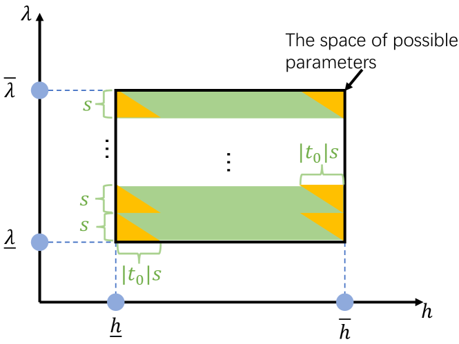
Figure 8: The construction for proof of Proposition 2 for shifted exponential distributions. We separate the space of possible parameters into two regions (yellow and green) and bound the attacker’s success rate on each region separately.

In Fig. 8, we separate the space of possible data parameters into two regions represented by yellow and green colors. The yellow regions $S_{yellow}$ constitute right triangles with height $s$ and width $\lvert t_{0}\rvert s$. The green region $S_{green}$ is the rest of the parameter space. The high-level idea of our proof is as follows. Note that for any parameter $\theta\in S_{green}$, there exists a $\mathcal{S}_{i,h}$ s.t. $\theta\in\mathcal{S}_{i,h}$ and $\mathcal{S}_{\mu,i}\subset S_{green}$. Therefore, we can bound the attack success rate if $\theta\in S_{green}$. At the same time, the probability of $\theta\in S_{yellow}$ is bounded. Therefore, we can bound the overall attacker’s success rate (i.e., $\Pi_{\epsilon,\omega_{\Theta}}$). More specifically, let the optimal attacker be $\hat{g}^{*}$. We have

$$\Pi_{\epsilon,\omega_{\Theta}}{} =\mathbb{P}\left(\hat{g}^{*}\left(\theta^{\prime}\right)\in\left[g\left(\theta\right)-\epsilon,g\left(\theta\right)+\epsilon\right]\right)$$

$$=\int_{\theta\in S_{green}}p(\theta)\mathbb{P}\left(\hat{g}^{*}\left(\theta^{\prime}\right)\in\left[g\left(\theta\right)-\epsilon,g\left(\theta\right)+\epsilon\right]\right)d\theta$$

$$\quad+\int_{\theta\in S_{yellow}}p(\theta)\mathbb{P}\left(\hat{g}^{*}\left(\theta^{\prime}\right)\in\left[g\left(\theta\right)-\epsilon,g\left(\theta\right)+\epsilon\right]\right)d\theta$$

$$<\frac{2\epsilon}{\lvert\ln\left(1-\alpha\right)+t_{0}\rvert s}+\frac{\lvert t_{0}\rvert s}{\overline{h}-\underline{h}}.$$

For the distortion, it is straightforward to get that $\Delta=\frac{s}{2}\left(t_{0}-1\right)+se^{-t_{0}}$ from Eq. 21, and $\Delta_{\text{opt}}>\left(\lceil{\frac{1}{\Pi_{\epsilon,\omega_{\Theta}}{}}}\rceil-1\right)\cdot 2\ratio\epsilon\geq 2\ratio\epsilon$, where is defined in Corollary 2. Denote $\zeta=\frac{2\epsilon}{\lvert\ln\left(1-\alpha\right)+t_{0}\rvert s}+\frac{\lvert t_{0}\rvert s}{\overline{h}-\underline{h}}-\Pi_{\epsilon,\omega_{\Theta}}$, we can get that $\left(\Pi_{\epsilon,\omega_{\Theta}}+\zeta-\frac{\lvert t_{0}\rvert s}{\overline{h}-\underline{h}}\right)\cdot\Delta=2\ratio\epsilon$ and

$$\Delta =\Delta_{\text{opt}}+\Delta-\Delta_{\text{opt}}$$

$$<\Delta_{\text{opt}}+\Delta-\left(\lceil{\frac{1}{\Pi_{\epsilon,\omega_{\Theta}}}}\rceil-1\right)\cdot 2\ratio\epsilon$$

$$\leq\Delta_{\text{opt}}+2\ratio\epsilon+\Delta-{{\frac{2\ratio\epsilon}{\Pi_{\epsilon,\omega_{\Theta}}}}}$$

$$=\Delta_{\text{opt}}+2\ratio\epsilon+\frac{\frac{\lvert t_{0}\rvert s}{\overline{h}-\underline{h}}-\zeta}{\frac{2\epsilon}{\lvert\ln\left(1-\alpha\right)+t_{0}\rvert s}+\frac{\lvert t_{0}\rvert s}{\overline{h}-\underline{h}}-\zeta}\cdot\Delta$$

$$<\Delta_{\text{opt}}+2\ratio\epsilon+\frac{\frac{\lvert t_{0}\rvert s}{\overline{h}-\underline{h}}}{\frac{2\epsilon}{\lvert\ln\left(1-\alpha\right)+t_{0}\rvert s}+\frac{\lvert t_{0}\rvert s}{\overline{h}-\underline{h}}}\cdot\Delta.$$

Therefore,

$$\Delta <\left(1+\frac{\lvert t_{0}\rvert\cdot\lvert\ln\left(1-\alpha\right)+t_{0}\rvert s^{2}}{2\epsilon\left(\overline{h}-\underline{h}\right)}\right)\left(\Delta_{\text{opt}}+2\ratio\epsilon\right)$$

$$\leq\left(2+\frac{\lvert t_{0}\rvert\cdot\lvert\ln\left(1-\alpha\right)+t_{0}\rvert s^{2}}{\epsilon\left(\overline{h}-\underline{h}\right)}\right)\Delta_{\text{opt}}.$$

$t_{0}$ is bounded when $\alpha\in\left[0,c_{1}\right]\cup\left[1-\frac{1}{e},c_{2}\right]$, where $c_{1}\in\left[0,1-\frac{1}{e}\right),c_{2}\in\left[1-\frac{1}{e},1\right)$. Therefore, when $\alpha\in[0.01,0.25]\cup[0.75,0.99]$, we can get that

$$\lim{\sup_{{\frac{s^{2}}{\overline{h}-\underline{h}}}\rightarrow 0}}\Delta<\lim{\sup_{{\frac{s^{2}}{\overline{h}-\underline{h}}}\rightarrow 0}}\left(2+\frac{\lvert t_{0}\rvert\cdot\lvert\ln\left(1-\alpha\right)+t_{0}\rvert s^{2}}{\epsilon\left(\overline{h}-\underline{h}\right)}\right)\Delta_{\text{opt}}<3\Delta_{\text{opt}}.$$

∎

C-E Proofs for the Surrogate Metrics

Secret=Mean: For any $p_{\mathcal{Y}}$, we have

$$\tilde{\Delta}=d_{\text{Wasserstein-1}}\left(p_{\mathcal{X}}\|p_{\mathcal{Y}}\right)\geq\left|\frac{1}{n}\sum_{i=1}^{n}x_{i}-\frac{1}{n}\sum_{i=1}^{n}y_{i}\right|=-\tilde{\Pi}_{\epsilon}.$$

For $p_{\mathcal{Y}}$ released from our mechanism (§ VI-C), we have

$$\tilde{\Delta}=d_{\text{Wasserstein-1}}\left(p_{\mathcal{X}}\|p_{\mathcal{Y}}\right)=\left|\frac{1}{n}\sum_{i=1}^{n}x_{i}-\frac{1}{n}\sum_{i=1}^{n}y_{i}\right|=-\tilde{\Pi}_{\epsilon}.$$

Appendix D Privacy-Distortion Performance of Data Release Mechanism with Relaxed Assumption

D-A Privacy-Distortion Performance of Mechanism 1 with Relaxed Assumption

We relax Assumption 1 as follows.

Assumption 3.

The distribution parameter vector $\theta$ can be written as $(u,v)$, where $u\in\mathbb{R}$, $v\in\mathbb{R}^{q-1}$, and for any $u\neq u^{\prime}$, $f_{X_{u,v}}\left(x\right)=f_{X_{u^{\prime},v}}\left(x-u^{\prime}+u\right)$. The prior over distribution parameters is $f_{U,V}\left(a,b\right)=f_{U}\left(a\right)\cdot f_{V}\left(b\right)$, where $\text{Supp}\left({U}\right)=\left[\underline{u},\overline{u}\right)$, and $f_{U}$ is $\mathcal{L}$-Lipschitz continuous and has lower bound $\underline{c}$.

Based on Assumption 3, the Privacy-distortion performance of Mechanism 1 is shown below.

Proposition 3.

Under Assumption 3, Mechanism 1 has $\Delta=\frac{s}{2}$ and $\Pi_{\epsilon,\omega_{\Theta}}{}\leq\frac{2\epsilon\left[\underline{c}+\mathcal{L}\left(s-x^{*}-\epsilon\right)\right]}{\underline{c}s+\frac{\mathcal{L}}{2}\left(s-x^{*}\right)^{2}}$, where $x^{*}=s+\frac{\underline{c}}{\mathcal{L}}-\epsilon-\sqrt{\left(\frac{\underline{c}}{\mathcal{L}}-\epsilon\right)^{2}+\frac{2\underline{c}s}{\mathcal{L}}}$.

Proof.

We first provide the following lemma.

Lemma 1.

For a $\mathcal{L}$-Lipschitz continuous function $f(x),x\in\left[\underline{x},\overline{x}\right]$, $\inf_{x\in\left[\underline{x},\overline{x}\right]}f(x)\geq\underline{c}\geq 0$, it satisfies

$$\sup_{x^{\prime}\in\left[\underline{x},\overline{x}-\delta\right]}\frac{\int_{x^{\prime}}^{x^{\prime}+\delta}f(x)\mathrm{d}x}{\int_{\underline{x}}^{\overline{x}}f(x)\mathrm{d}x}\leq\frac{\delta\left[\underline{c}+\mathcal{L}\left(\overline{x}-x^{*}-\frac{\delta}{2}\right)\right]}{\underline{c}\left(\overline{x}-\underline{x}\right)+\frac{\mathcal{L}}{2}\left(\overline{x}-x^{*}\right)^{2}},$$

where $x^{*}=\overline{x}+\frac{\underline{c}}{\mathcal{L}}-\frac{\delta}{2}-\sqrt{\left(\frac{\underline{c}}{\mathcal{L}}-\frac{\delta}{2}\right)^{2}+\frac{2\underline{c}\left(\overline{x}-\underline{x}\right)}{\mathcal{L}}}$.

For any released parameter $\theta^{\prime}=(u^{\prime},v^{\prime})$, there exists $i\in\left\{0,...,N-1\right\}$ such that $u^{\prime}=\underline{u}+\left(i+0.5\right)\cdot s$. We have

$$\sup_{\hat{g}} \ \mathbb{P}\left(\hat{g}\left(\theta^{\prime}\right)\in\left[g\left(\theta\right)-\epsilon,g\left(\theta\right)+\epsilon\right]\big{|}\theta^{\prime}\right)$$

$$=\sup_{\hat{g}}\int_{\underline{u}+i\cdot s}^{\underline{u}+\left(i+1\right)\cdot s}f_{U|U^{\prime}}\left(u|u^{\prime}\right)\cdot\int_{u-\epsilon}^{u+\epsilon}f_{\hat{g}\left(u^{\prime},v^{\prime}\right)}\left(h\right)\ \mathrm{d}h\ \mathrm{d}u$$

$$=\sup_{\hat{g}}\int_{\underline{u}+i\cdot s-\epsilon}^{\underline{u}+\left(i+1\right)\cdot s+\epsilon}f_{\hat{g}\left(u^{\prime},v^{\prime}\right)}(h)\cdot\int_{\hat{g}\left(f_{X_{u^{\prime},v^{\prime}}}\right)-\epsilon}^{\hat{g}\left(f_{X_{u^{\prime},v^{\prime}}}\right)+\epsilon}f_{U|U^{\prime}}\left(u|u^{\prime}\right)\ \mathrm{d}u\ \mathrm{d}h.$$

For $\int_{\hat{g}\left(f_{X_{u^{\prime},v^{\prime}}}\right)-\epsilon}^{\hat{g}\left(f_{X_{u^{\prime},v^{\prime}}}\right)+\epsilon}f_{U|U^{\prime}}\left(u|u^{\prime}\right)\ \mathrm{d}u$, denote

$$x_{1}=\max\left(0,\hat{g}\left(f_{X_{u^{\prime},v^{\prime}}}\right)-\epsilon-\underline{u}-i\cdot s\right),$$

$$x_{2}=\min\left(\hat{g}\left(f_{X_{u^{\prime},v^{\prime}}}\right)+\epsilon-\underline{u}-i\cdot s,s\right),$$

we have

$$\int_{\hat{g}\left(f_{X_{u^{\prime},v^{\prime}}}\right)-\epsilon}^{\hat{g}\left(f_{X_{u^{\prime},v^{\prime}}}\right)+\epsilon}f_{U|U^{\prime}}\left(u|u^{\prime}\right)\ \mathrm{d}u=\frac{\int_{x_{1}}^{x_{2}}f_{U}\left(\underline{u}+i\cdot s+x\right)\ \mathrm{d}x}{\int_{0}^{s}f_{U}\left(\underline{u}+i\cdot s+x\right)\ \mathrm{d}x}.$$

$f_{U}\left(\underline{u}+i\cdot s+x\right)$ is $\mathcal{L}$-Lipschitz and has lower bound $\underline{c}$. $x_{2}-x_{1}\leq 2\epsilon$ and $x_{1},x_{2}\in\left[0,s\right]$. According to Lemma 1, we have

$$\int_{\hat{g}\left(f_{X_{u^{\prime},v^{\prime}}}\right)-\epsilon}^{\hat{g}\left(f_{X_{u^{\prime},v^{\prime}}}\right)+\epsilon}f_{U|U^{\prime}}\left(u|u^{\prime}\right)\ \mathrm{d}u =\frac{\int_{x_{1}}^{x_{2}}f_{U}\left(\underline{u}+i\cdot s+x\right)\ \mathrm{d}x}{\int_{0}^{s}f_{U}\left(\underline{u}+i\cdot s+x\right)\ \mathrm{d}x}$$

$$\leq\frac{2\epsilon\left[\underline{c}+\mathcal{L}\left(s-x^{*}-\epsilon\right)\right]}{\underline{c}s+\frac{\mathcal{L}}{2}\left(s-x^{*}\right)^{2}},$$

where $x^{*}=s+\frac{\underline{c}}{\mathcal{L}}-\epsilon-\sqrt{\left(\frac{\underline{c}}{\mathcal{L}}-\epsilon\right)^{2}+\frac{2\underline{c}s}{\mathcal{L}}}$.

Therefore, we can get that

$$\sup_{\hat{g}}\ \mathbb{P}\left(\hat{g}\left(\theta^{\prime}\right)\in\left[g\left(\theta\right)-\epsilon,g\left(\theta\right)+\epsilon\right]\big{|}\theta^{\prime}\right)$$

$$\leq\sup_{\hat{g}}\int_{\underline{u}+i\cdot s-\epsilon}^{\underline{u}+\left(i+1\right)\cdot s+\epsilon}\frac{2\epsilon\left[\underline{c}+\mathcal{L}\left(s-x^{*}-\epsilon\right)\right]}{\underline{c}s+\frac{\mathcal{L}}{2}\left(s-x^{*}\right)^{2}}\cdot f_{\hat{g}\left(u^{\prime},v^{\prime}\right)}(h)\ \mathrm{d}h$$

$$\leq\frac{2\epsilon\left[\underline{c}+\mathcal{L}\left(s-x^{*}-\epsilon\right)\right]}{\underline{c}s+\frac{\mathcal{L}}{2}\left(s-x^{*}\right)^{2}}.$$

Therefore, we have

$$\Pi_{\epsilon,\omega_{\Theta}}{} =\sup_{\hat{g}}\mathbb{P}\left(\hat{g}\left(\theta^{\prime}\right)\in\left[g\left(\theta\right)-\epsilon,g\left(\theta\right)+\epsilon\right]\right)$$

$$=\sup_{\hat{g}}\mathbb{E}\left(\mathbb{P}\left(\hat{g}\left(\theta^{\prime}\right)\in\left[g\left(\theta\right)-\epsilon,g\left(\theta\right)+\epsilon\right]\bigg{|}\theta^{\prime}\right)\right)$$

$$=\mathbb{E}\left(\sup_{\hat{g}}\mathbb{P}\left(\hat{g}\left(\theta^{\prime}\right)\in\left[g\left(\theta\right)-\epsilon,g\left(\theta\right)+\epsilon\right]\bigg{|}\theta^{\prime}\right)\right)$$

$$\leq\frac{2\epsilon\left[\underline{c}+\mathcal{L}\left(s-x^{*}-\epsilon\right)\right]}{\underline{c}s+\frac{\mathcal{L}}{2}\left(s-x^{*}\right)^{2}}.$$

For the distortion, we can easily get that $\Delta=\frac{s}{2}$. ∎

D-A1 Proof of Lemma 1

Without loss of generality, we assume that $f(\overline{x})\geq f(\underline{x})$. Based on simple geometric analysis, we can get that when $\frac{\int_{x^{\prime}}^{x^{\prime}+\delta}f(x)\mathrm{d}x}{\int_{\underline{x}}^{\overline{x}}f(x)\mathrm{d}x}$ achieves supremum, as illustrated in Fig. 9, $f(\underline{x})=\underline{c}$, $x^{\prime}=\overline{x}-\delta$, and $f(\overline{x})=\underline{x}+\mathcal{L}\left(\overline{x}-x^{\prime\prime}\right)$, where $x^{\prime\prime}\in\left[\underline{x},x^{\prime}\right]$.

Figure 9: Illustration of $f(x)$ when $\frac{\int_{x^{\prime}}^{x^{\prime}+\delta}f(x)\mathrm{d}x}{\int_{\underline{x}}^{\overline{x}}f(x)\mathrm{d}x}$ achieves supremum.

In this case, we can get that

$$\frac{\int_{\overline{x}-\delta}^{\overline{x}}f(x)\mathrm{d}x}{\int_{\underline{x}}^{\overline{x}}f(x)\mathrm{d}x}=\frac{\delta\left[\underline{c}+\mathcal{L}\left(\overline{x}-x^{\prime\prime}-\frac{\delta}{2}\right)\right]}{\underline{c}\left(\overline{x}-\underline{x}\right)+\frac{\mathcal{L}}{2}\left(\overline{x}-x^{\prime\prime}\right)^{2}}\triangleq h\left(x^{\prime\prime}\right),$$

where $x^{\prime\prime}\in\left[\underline{x},x^{\prime}\right]$. When $x^{\prime\prime}=\overline{x}+\frac{\underline{c}}{\mathcal{L}}-\frac{\delta}{2}-\sqrt{\left(\frac{\underline{c}}{\mathcal{L}}-\frac{\delta}{2}\right)^{2}+\frac{2\underline{c}\left(\overline{x}-\underline{x}\right)}{\mathcal{L}}}\triangleq x^{*}$, $h(x^{\prime\prime})$ achieves supremum. Therefore, we have

$$\sup_{x^{\prime}\in\left[\underline{x},\overline{x}-\delta\right]}\frac{\int_{x^{\prime}}^{x^{\prime}+\delta}f(x)\mathrm{d}x}{\int_{\underline{x}}^{\overline{x}}f(x)\mathrm{d}x} \leq\sup_{f}\sup_{x^{\prime}\in\left[\underline{x},\overline{x}-\delta\right]}\frac{\int_{x^{\prime}}^{x^{\prime}+\delta}f(x)\mathrm{d}x}{\int_{\underline{x}}^{\overline{x}}f(x)\mathrm{d}x}$$

$$=\frac{\delta\left[\underline{c}+\mathcal{L}\left(\overline{x}-x^{*}-\frac{\delta}{2}\right)\right]}{\underline{c}\left(\overline{x}-\underline{x}\right)+\frac{\mathcal{L}}{2}\left(\overline{x}-x^{*}\right)^{2}}.$$

D-B Privacy-Distortion Performance of Mechanism 2 with Relaxed Assumption

We relax Assumption 2 as follows.

Assumption 4.

The prior over distribution parameters as specified below.

• Exponential: $\text{Supp}\left({\lambda}\right)=\left[\underline{\lambda},\overline{\lambda}\right)$, and $f_{\lambda}$ is $\mathcal{L}$-Lipschitz continuous and has lower bound $\underline{c}$.

• Shifted exponential: $\text{Supp}\left({\lambda,h}\right)=\left\{(a,b)|a\in\left[\underline{\lambda},\overline{\lambda}\right),b\in\left[\underline{h},\overline{h}\right)\right\}$, $f_{\lambda,h}\left(a,b\right)=f_{\lambda}\left(a\right)\cdot f_{h}\left(b\right)$, and $f_{\lambda}$ (resp. $f_{h}$) is $\mathcal{L}_{\lambda}$-Lipschitz (resp. $\mathcal{L}_{h}$-Lipschitz) and has lower bound $\frac{k_{\lambda}}{\overline{\mu}-\underline{\mu}}$ with $k_{\lambda}\in(0,1]$ (resp. $\frac{k_{h}}{\overline{\sigma}-\underline{\sigma}}$ with $k_{h}\in(0,1]$).

Based on Assumption 4, the Privacy-distortion performance of Mechanism 2 is shown below.

Proposition 4.

Under Assumption 4, Mechanism 2 has the following $\Delta$ and $\Pi_{\epsilon,\omega_{\Theta}}{}$ value/bound.

• Exponential:

  $$\Delta =\frac{1}{2}s,$$

  $$\Pi_{\epsilon,\omega_{\Theta}} \leq\frac{\frac{2\epsilon}{-\ln\left(1-\alpha\right)}\cdot\left[\underline{c}+\mathcal{L}\left(s-x^{*}+\frac{\epsilon}{\ln\left(1-\alpha\right)}\right)\right]}{\underline{c}s+\frac{\mathcal{L}}{2}\left(s-x^{*}\right)^{2}},$$

  where $x^{*}=s+\frac{\underline{c}}{\mathcal{L}}+\frac{\epsilon}{\ln\left(1-\alpha\right)}-\sqrt{\left(\frac{\underline{c}}{\mathcal{L}}+\frac{\epsilon}{\ln\left(1-\alpha\right)}\right)^{2}+\frac{2\underline{c}s}{\mathcal{L}}}$.

• Shifted exponential:

  $$\Delta =\frac{s}{2}\left(t_{0}-1\right)+se^{-t_{0}},$$

  $$\Pi_{\epsilon,\omega_{\Theta}} <\frac{\frac{2\epsilon}{\lvert\ln\left(1-\alpha\right)+t_{0}\rvert}\cdot\left[\underline{c}+\mathcal{L}_{\lambda,h}\left(\frac{s}{2}-t^{*}-\frac{\epsilon}{\lvert\ln\left(1-\alpha\right)+t_{0}\rvert}\right)\right]}{\underline{c}s+\frac{\mathcal{L}_{\lambda,h}}{2}\left(\frac{s}{2}-t^{*}\right)^{2}}+$$

  $$M\left(\overline{h}-\underline{h},\frac{k_{h}}{\overline{h}-\underline{h}},\mathcal{L}_{h},1\right)\cdot M\left(\overline{\lambda}-\underline{\lambda},\frac{k_{\lambda}}{\overline{\lambda}-\underline{\lambda}},\mathcal{L}_{\lambda},1\right)\cdot\left(\overline{\lambda}-\underline{\lambda}\right)\lvert t_{0}\rvert s,$$

  where $\underline{c}=\frac{k_{h}k_{\lambda}}{\left(\overline{h}-\underline{h}\right)\cdot\left(\overline{\lambda}-\underline{\lambda}\right)}$, function $M$ satisfies

  $$M\left(x,c,\mathcal{L},\mathcal{A}\right)=\begin{cases}\frac{\mathcal{A}}{x}+\frac{\mathcal{L}x}{2},&\text{if }c\leq\frac{\mathcal{A}}{x}-\frac{\mathcal{L}x}{2}\\ c+\sqrt{2\mathcal{L}\left(\mathcal{A}-cx\right)},&\text{if }c>\frac{\mathcal{A}}{x}-\frac{\mathcal{L}x}{2}\end{cases},$$

  $\mathcal{L}_{\lambda,h}=\mathcal{L}_{\lambda}M\left(\frac{\overline{h}-\underline{h}}{\lvert t_{0}\rvert},\frac{k_{h}}{\overline{h}-\underline{h}},\lvert t_{0}\rvert\mathcal{L}_{h},\frac{1}{\lvert t_{0}\rvert}\right)+\lvert t_{0}\rvert\mathcal{L}_{h}M\left(\overline{\lambda}-\underline{\lambda},\frac{k_{\lambda}}{\overline{\lambda}-\underline{\lambda}},\mathcal{L}_{\lambda},1\right)$, and
  $t^{*}=\frac{s}{2}+\frac{\underline{c}}{\mathcal{L}_{\lambda,h}}-\frac{\epsilon}{\lvert\ln\left(1-\alpha\right)+t_{0}\rvert}-\sqrt{\left(\frac{\underline{c}}{\mathcal{L}_{\lambda,h}}-\frac{\epsilon}{\lvert\ln\left(1-\alpha\right)+t_{0}\rvert}\right)^{2}+\frac{2\underline{c}s}{\mathcal{L}_{\lambda,h}}}$.

The $t_{0}$ parameter is defined in Mechanism 2.

D-B1 Proof of Proposition 4 for Exponential Distribution

It is straightforward to get the formula for $\Delta$ from Eq. 20. Here we focus on the proof for $\Pi_{\epsilon,\omega_{\Theta}}$.

Similar to the proof in § D-A, according to Lemma 1, we have

$$\Pi_{\epsilon,\omega_{\Theta}}{} =\mathbb{E}\left(\sup_{\hat{g}}\mathbb{P}\left(\hat{g}\left(\theta^{\prime}\right)\in\left[g\left(\theta\right)-\epsilon,g\left(\theta\right)+\epsilon\right]\bigg{|}\theta^{\prime}\right)\right)$$

$$\leq\sup_{i\in\mathbb{N},t^{\prime}\in\mathbb{R}}\frac{\int_{\max\left\{0,t^{\prime}\right\}}^{\min\left\{s,t^{\prime}-\frac{2\epsilon}{\ln\left(1-\alpha\right)}\right\}}f_{\lambda}\left(\underline{\lambda}+i\cdot s+t\right)\mathrm{d}t}{\int_{0}^{s}f_{\lambda}\left(\underline{\lambda}+i\cdot s+t\right)\mathrm{d}t}$$

$$\leq\frac{\frac{2\epsilon}{-\ln\left(1-\alpha\right)}\cdot\left[\underline{c}+\mathcal{L}\left(s-x^{*}+\frac{\epsilon}{\ln\left(1-\alpha\right)}\right)\right]}{\underline{c}s+\frac{\mathcal{L}}{2}\left(s-x^{*}\right)^{2}},$$

where $x^{*}=s+\frac{\underline{c}}{\mathcal{L}}+\frac{\epsilon}{\ln\left(1-\alpha\right)}-\sqrt{\left(\frac{\underline{c}}{\mathcal{L}}+\frac{\epsilon}{\ln\left(1-\alpha\right)}\right)^{2}+\frac{2\underline{c}s}{\mathcal{L}}}$.

D-B2 Proof of Proposition 4 for Shifted Exponential Distribution

It is straightforward to get the formula for $\Delta$ from Eq. 21. Here we focus on the proof for $\Pi_{\epsilon,\omega_{\Theta}}$.

According to LABEL:eqn:green-yellow, we can bound the attack success rate $\Pi_{\epsilon,\omega_{\Theta}}$ as

$$\Pi_{\epsilon,\omega_{\Theta}}{}<\sup_{\theta\in S_{green}}\mathbb{P}\left(\hat{g}^{*}\left(\theta^{\prime}\right)\in\left[g\left(\theta\right)-\epsilon,g\left(\theta\right)+\epsilon\right]\right)+\int_{\theta\in S_{yellow}}p(\theta)d\theta.$$

As for the first term $\sup_{\theta\in S_{green}}\mathbb{P}\left(\hat{g}^{*}\left(\theta^{\prime}\right)\in\left[g\left(\theta\right)-\epsilon,g\left(\theta\right)+\epsilon\right]\right)$, we can get that

$$\sup_{\theta\in S_{green}}\mathbb{P}\left(\hat{g}^{*}\left(\theta^{\prime}\right)\in\left[g\left(\theta\right)-\epsilon,g\left(\theta\right)+\epsilon\right]\right)$$

$$=\sup_{i\in\mathbb{N},h,t^{\prime}\in\mathbb{R}}\frac{\int_{\max\left\{-\frac{s}{2},t^{\prime}\right\}}^{\min\left\{\frac{s}{2},t^{\prime}+\frac{2\epsilon}{\lvert\ln\left(1-\alpha\right)+t_{0}\rvert}\right\}}f_{\lambda,h}\left(\underline{\lambda}+\left(i+0.5\right)\cdot s+t,h-t_{0}\cdot t\right)\mathrm{d}t}{\int_{-\frac{s}{2}}^{\frac{s}{2}}f_{\lambda,h}\left(\underline{\lambda}+\left(i+0.5\right)\cdot s+t,h-t_{0}\cdot t\right)\mathrm{d}t}.$$

To analyze the above term, we provide the following lemma.

Lemma 2.

For a $\mathcal{L}$-Lipschitz continuous function $f(x),x\in\left[\underline{x},\overline{x}\right]$, if $\int_{\underline{x}}^{\overline{x}}f(x)\mathrm{d}x=\mathcal{A}$ and $\inf_{x\in\left[\underline{x},\overline{x}\right]}f(x)\geq\underline{c}$, it satisfies

$$\sup_{x\in\left[\underline{x},\overline{x}\right]}f(x) \leq\begin{cases}\frac{\mathcal{A}}{\overline{x}-\underline{x}}+\frac{\mathcal{L}\left(\overline{x}-\underline{x}\right)}{2},&\text{if }\underline{c}\leq\frac{\mathcal{A}}{\overline{x}-\underline{x}}-\frac{\mathcal{L}\left(\overline{x}-\underline{x}\right)}{2}\\ \underline{c}+\sqrt{2\mathcal{L}\left(\mathcal{A}-\underline{c}\left(\overline{x}-\underline{x}\right)\right)},&\text{if }\underline{c}>\frac{\mathcal{A}}{\overline{x}-\underline{x}}-\frac{\mathcal{L}\left(\overline{x}-\underline{x}\right)}{2}\end{cases}$$

$$\triangleq M\left(\overline{x}-\underline{x},\underline{c},\mathcal{L},\mathcal{A}\right).$$

The proof is in § D-B3.

Since $f_{\lambda,h}\left(\underline{\lambda}+\left(i+0.5\right)\cdot s+t,h-t_{0}\cdot t\right)=f_{\lambda}\left(\underline{\lambda}+\left(i+0.5\right)\cdot s+t\right)\cdot f_{h}\left(h-t_{0}\cdot t\right)$, according to Lemma 2, we can get that $f_{\lambda,h}$ is $\mathcal{L}_{\lambda,h}$-Lipschitz continuous, where

$$\mathcal{L}_{\lambda,h}=\mathcal{L}_{\lambda}\cdot M\left(\frac{\overline{h}-\underline{h}}{\lvert t_{0}\rvert},\frac{k_{h}}{\overline{h}-\underline{h}},\lvert t_{0}\rvert\mathcal{L}_{h},\frac{1}{\lvert t_{0}\rvert}\right)+\lvert t_{0}\rvert\mathcal{L}_{h}\cdot M\left(\overline{\lambda}-\underline{\lambda},\frac{k_{\lambda}}{\overline{\lambda}-\underline{\lambda}},\mathcal{L}_{\lambda},1\right).$$

We can also get that

$$\inf_{a\in\left[\underline{\lambda},\overline{\lambda}\right),b\in\left[\underline{h},\overline{h}\right)}f_{\lambda,h}\left(a,b\right)\geq\frac{k_{h}k_{\lambda}}{\left(\overline{h}-\underline{h}\right)\cdot\left(\overline{\lambda}-\underline{\lambda}\right)}\triangleq\underline{c}.$$

Therefore, according to Lemma 1, we can get that

$$\sup_{\theta\in S_{green}}\mathbb{P}\left(\hat{g}^{*}\left(\theta^{\prime}\right)\in\left[g\left(\theta\right)-\epsilon,g\left(\theta\right)+\epsilon\right]\right)$$

$$=\sup_{i\in\mathbb{N},h,t^{\prime}\in\mathbb{R}}\frac{\int_{\max\left\{-\frac{s}{2},t^{\prime}\right\}}^{\min\left\{\frac{s}{2},t^{\prime}+\frac{2\epsilon}{\lvert\ln\left(1-\alpha\right)+t_{0}\rvert}\right\}}f_{\lambda,h}\left(\underline{\lambda}+\left(i+0.5\right)\cdot s+t,h-t_{0}\cdot t\right)\mathrm{d}t}{\int_{-\frac{s}{2}}^{\frac{s}{2}}f_{\lambda,h}\left(\underline{\lambda}+\left(i+0.5\right)\cdot s+t,h-t_{0}\cdot t\right)\mathrm{d}t}$$

$$\leq\frac{\frac{2\epsilon}{\lvert\ln\left(1-\alpha\right)+t_{0}\rvert}\cdot\left[\underline{c}+\mathcal{L}_{\lambda,h}\left(\frac{s}{2}-t^{*}-\frac{\epsilon}{\lvert\ln\left(1-\alpha\right)+t_{0}\rvert}\right)\right]}{\underline{c}s+\frac{\mathcal{L}_{\lambda,h}}{2}\left(\frac{s}{2}-t^{*}\right)^{2}},$$

where $t^{*}=\frac{s}{2}+\frac{\underline{c}}{\mathcal{L}_{\lambda,h}}-\frac{\epsilon}{\lvert\ln\left(1-\alpha\right)+t_{0}\rvert}-\sqrt{\left(\frac{\underline{c}}{\mathcal{L}_{\lambda,h}}-\frac{\epsilon}{\lvert\ln\left(1-\alpha\right)+t_{0}\rvert}\right)^{2}+\frac{2\underline{c}s}{\mathcal{L}_{\lambda,h}}}$, $\mathcal{L}_{\lambda,h}=\mathcal{L}_{\lambda}\cdot M\left(\frac{\overline{h}-\underline{h}}{\lvert t_{0}\rvert},\frac{k_{h}}{\overline{h}-\underline{h}},\lvert t_{0}\rvert\mathcal{L}_{h},\frac{1}{\lvert t_{0}\rvert}\right)+\lvert t_{0}\rvert\mathcal{L}_{h}\cdot M\left(\overline{\lambda}-\underline{\lambda},\frac{k_{\lambda}}{\overline{\lambda}-\underline{\lambda}},\mathcal{L}_{\lambda},1\right)$, and $\underline{c}=\frac{k_{h}k_{\lambda}}{\left(\overline{h}-\underline{h}\right)\cdot\left(\overline{\lambda}-\underline{\lambda}\right)}$.

As for $\int_{\theta\in S_{yellow}}p(\theta)d\theta$, we have

$$\int_{\theta\in S_{yellow}}p(\theta)d\theta$$

$$\leq M\left(\overline{h}-\underline{h},\frac{k_{h}}{\overline{h}-\underline{h}},\mathcal{L}_{h},1\right)\cdot M\left(\overline{\lambda}-\underline{\lambda},\frac{k_{\lambda}}{\overline{\lambda}-\underline{\lambda}},\mathcal{L}_{\lambda},1\right)\cdot\int_{\theta\in S_{yellow}}d\theta$$

$$=M\left(\overline{h}-\underline{h},\frac{k_{h}}{\overline{h}-\underline{h}},\mathcal{L}_{h},1\right)\cdot M\left(\overline{\lambda}-\underline{\lambda},\frac{k_{\lambda}}{\overline{\lambda}-\underline{\lambda}},\mathcal{L}_{\lambda},1\right)\cdot\left(\overline{\lambda}-\underline{\lambda}\right)\lvert t_{0}\rvert s.$$

Above all, we can get that

$$\Pi_{\epsilon,\omega_{\Theta}}{} <\sup_{\theta\in S_{green}}\mathbb{P}\left(\hat{g}^{*}\left(\theta^{\prime}\right)\in\left[g\left(\theta\right)-\epsilon,g\left(\theta\right)+\epsilon\right]\right)+\int_{\theta\in S_{yellow}}p(\theta)d\theta.$$

$$\leq\frac{\frac{2\epsilon}{\lvert\ln\left(1-\alpha\right)+t_{0}\rvert}\cdot\left[\underline{c}+\mathcal{L}_{\lambda,h}\left(\frac{s}{2}-t^{*}-\frac{\epsilon}{\lvert\ln\left(1-\alpha\right)+t_{0}\rvert}\right)\right]}{\underline{c}s+\frac{\mathcal{L}_{\lambda,h}}{2}\left(\frac{s}{2}-t^{*}\right)^{2}}+$$

$$M\left(\overline{h}-\underline{h},\frac{k_{h}}{\overline{h}-\underline{h}},\mathcal{L}_{h},1\right)\cdot M\left(\overline{\lambda}-\underline{\lambda},\frac{k_{\lambda}}{\overline{\lambda}-\underline{\lambda}},\mathcal{L}_{\lambda},1\right)\cdot\left(\overline{\lambda}-\underline{\lambda}\right)\lvert t_{0}\rvert s,$$

where $M(\cdot,\cdot,\cdot,\cdot),\underline{c},\mathcal{L}_{\lambda,h},t^{*}$ are defined as above.

D-B3 Proof of Lemma 2

Without loss of generality, we assume that $f(\overline{x})\geq f(\underline{x})$. Based on simple geometric analysis, we can get that there are two patterns when $\sup_{x\in\left[\underline{x},\overline{x}\right]}f(x)$ achieves supremum, which are shown in Fig. 10.

(a) Pattern 1.

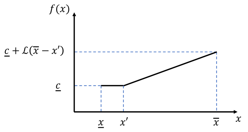
(b) Pattern 2.

Figure 10: Two patterns when $\sup_{x\in\left[\underline{x},\overline{x}\right]}f(x)$ achieves supremum.

For pattern 1, $f(\underline{x})=c_{1}\geq\underline{c}$, $f(\overline{x})=c_{1}+\mathcal{L}(\overline{x}-\underline{x})$, and $\int_{\underline{x}}^{\overline{x}}f(x)\mathrm{d}x=\left(c_{1}+\frac{\mathcal{L}}{2}(\overline{x}-\underline{x})\right)\cdot\left(\overline{x}-\underline{x}\right)=\mathcal{A}$. Therefore, when $\underline{c}\leq\frac{\mathcal{A}}{\overline{x}-\underline{x}}-\frac{\mathcal{L}\left(\overline{x}-\underline{x}\right)}{2}$, we have

$$\sup_{f}\sup_{x\in\left[\underline{x},\overline{x}\right]}f(x)=c_{1}+\mathcal{L}(\overline{x}-\underline{x})=\frac{\mathcal{A}}{\overline{x}-\underline{x}}+\frac{\mathcal{L}\left(\overline{x}-\underline{x}\right)}{2}.$$

For pattern 2, $f(\underline{x})=\underline{c}$, $f(\overline{x})=\underline{c}+\mathcal{L}(\overline{x}-x^{\prime})$, where $x^{\prime}\in\left(\underline{x},\overline{x}\right]$, and $\int_{\underline{x}}^{\overline{x}}f(x)\mathrm{d}x=\underline{c}(\overline{x}-\underline{x})+\frac{\mathcal{L}}{2}\left(\overline{x}-x^{\prime}\right)^{2}=\mathcal{A}$. Therefore, when $\underline{c}>\frac{\mathcal{A}}{\overline{x}-\underline{x}}-\frac{\mathcal{L}\left(\overline{x}-\underline{x}\right)}{2}$, we have

$$\sup_{f}\sup_{x\in\left[\underline{x},\overline{x}\right]}f(x)=\underline{c}+\mathcal{L}(\overline{x}-x^{\prime})=\underline{c}+\sqrt{2\mathcal{L}\left(\mathcal{A}-\underline{c}\left(\overline{x}-\underline{x}\right)\right)}.$$

Above all, we can get that

$$\sup_{x\in\left[\underline{x},\overline{x}\right]}f(x) \leq\sup_{f}\sup_{x\in\left[\underline{x},\overline{x}\right]}f(x)$$

$$=\begin{cases}\frac{\mathcal{A}}{\overline{x}-\underline{x}}+\frac{\mathcal{L}\left(\overline{x}-\underline{x}\right)}{2},&\text{if }\underline{c}\leq\frac{\mathcal{A}}{\overline{x}-\underline{x}}-\frac{\mathcal{L}\left(\overline{x}-\underline{x}\right)}{2}\\ \underline{c}+\sqrt{2\mathcal{L}\left(\mathcal{A}-\underline{c}\left(\overline{x}-\underline{x}\right)\right)},&\text{if }\underline{c}>\frac{\mathcal{A}}{\overline{x}-\underline{x}}-\frac{\mathcal{L}\left(\overline{x}-\underline{x}\right)}{2}\end{cases}.$$

Appendix E Discrete Distribution with Secret = Mean

Here, we consider three typical examples of discrete distributions: geometric distributions, binomial distributions, and Poisson distributions with parameter $\theta$. More specifically, the original distribution is

$$\mathbb{P}\left(X_{\theta}=k\right)=\begin{cases}\left(1-\theta\right)^{k}\theta&\text{(geometric distribution)}\\ \binom{n}{k}\theta^{k}\left(1-\theta\right)^{n-k}&\text{(binomial distribution)}\\ \frac{\theta^{k}e^{-\theta}}{k!}&\text{(Poisson distribution)}\end{cases}$$

where $n$ standards for the number of trials in binomial distribution. The support of the parameter is $\text{Supp}\left(\Theta\right)=\left\{X_{\theta}:\theta\in\left(\underline{\theta},\overline{\theta}\right]\right\}$ where $\left(\underline{\theta},\overline{\theta}\right]\subseteq\left(0,1\right)$ for geometric distribution and binomial distribution, and $\left(\underline{\theta},\overline{\theta}\right]\subseteq\left(0,\infty\right)$ for Poisson distribution.

We first analyze the lower bound.

Corollary 3 (Privacy lower bound, secret = mean of a discrete distribution).

Consider the secret function $g\left(\theta\right)=\sum_{x}xf_{X_{\theta}}\left(x\right)$. For any $T\in\left(0,1\right)$, when $\Pi_{\epsilon,\omega_{\Theta}}\leq T$, we have $\Delta>\left(\lceil{\frac{1}{T}}\rceil-1\right)\cdot 2\ratio\epsilon$, where the value of depends on the type of the distributions:

• Geometric:

  $$\ratio=\inf_{\underline{\theta}<\theta_{1}<\theta_{2}\leq\overline{\theta}}\frac{\left(1-\theta_{2}\right)^{h\left(\theta_{1},\theta_{2}\right)}-\left(1-\theta_{1}\right)^{h\left(\theta_{1},\theta_{2}\right)}}{2\left(\frac{1}{\theta_{2}}-\frac{1}{\theta_{1}}\right)}~{},$$

  where $h\left(\theta_{1},\theta_{2}\right)=\lfloor{\frac{\log\left(\theta_{2}\right)-\log\left(\theta_{1}\right)}{\log\left(1-\theta_{1}\right)-\log\left(1-\theta_{2}\right)}}\rfloor+1$.

• Binomial:

  $$\ratio=\inf_{\underline{\theta}<\theta_{1}<\theta_{2}\leq\overline{\theta}}$$

  where $h\left(\theta_{1},\theta_{2}\right)=\lfloor{k^{\prime}}\rfloor$, $k^{\prime}=n\ln\left(\frac{1-\theta_{2}}{1-\theta_{1}}\right)\Big{/}\ln\left({\frac{\theta_{1}\left(1-\theta_{2}\right)}{\theta_{2}\left(1-\theta_{1}\right)}}\right)$, and $I$ represents the regularized incomplete beta function.

• Poisson:

  $$\ratio=\inf_{\underline{\theta}<\theta_{1}<\theta_{2}\leq\overline{\theta}}\frac{Q\left(h\left(\theta_{1},\theta_{2}\right),\theta_{2}\right)-Q\left(h\left(\theta_{1},\theta_{2}\right),\theta_{1}\right)}{2\left(\theta_{1}-\theta_{2}\right)},$$

  where $h\left(\theta_{1},\theta_{2}\right)=\lfloor{\frac{\theta_{1}-\theta_{2}}{\ln\left(\theta_{1}\right)-\ln\left(\theta_{2}\right)}}\rfloor+1$ and $Q$ is the regularized gamma function.

The proof is in § E-A. The above lower bounds can be computed numerically.

Since these distributions only have one parameter, we can use Algorithm 1 and Algorithm 3 to derive a data release mechanism. The performance of greedy-based and dynamic-programming-based data release mechanisms for each distribution is shown in Fig. 11.

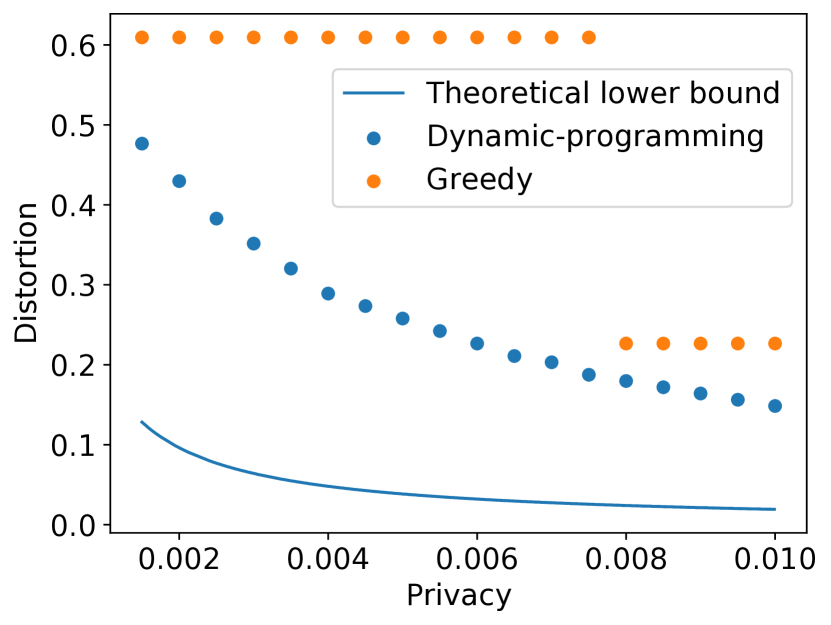
(a) Distribution = Geometric

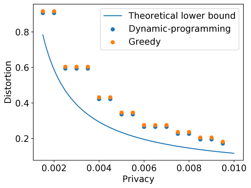
(b) Distribution = Binomial

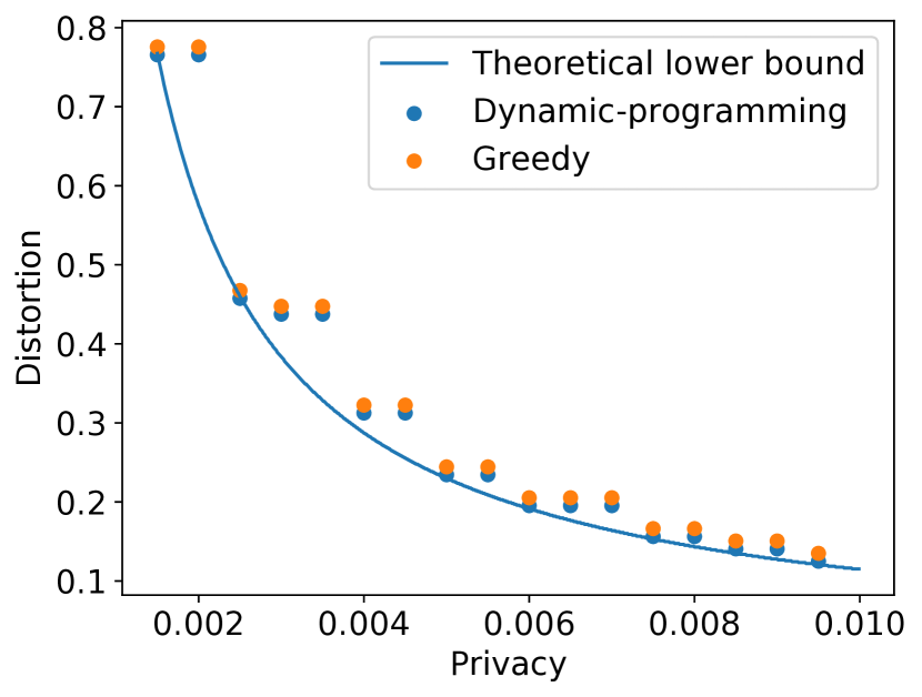
(c) Distribution = Poisson

Figure 11: Privacy-distortion performance of Algorithm 1 and Algorithm 3 for geometric, binomial and Poisson distribution when secret = mean.

As we can observe, the distortion that dynamic-programming-based data release mechanism achieves it is always smaller than or equal to that of the greedy-based data release mechanism.

E-A Proof of Corollary 3

E-A1 Geometric Distribution

Proof.

Let $X_{\theta_{1}}$ and $X_{\theta_{2}}$ be two Geometric random variables with parameters $\theta_{1}$ and $\theta_{2}$ respectively. We assume that $\theta_{1}>\theta_{2}$ without loss of generality. Let $k^{\prime}$ satisfy $\left(1-\theta_{1}\right)^{k^{\prime}}\theta_{1}=\left(1-\theta_{2}\right)^{k^{\prime}}\theta_{2}$ and $k_{0}=\lfloor{k^{\prime}}\rfloor+1$. Then we can get that

$$D\left(X_{\theta_{1}},X_{\theta_{2}}\right) =\frac{1}{2}d_{\text{TV}}\left(\omega_{X_{\theta_{1}}}\|\omega_{X_{\theta_{2}}}\right)$$

$$=\frac{1}{2}\left(1-\theta_{2}\right)^{k_{0}}-\frac{1}{2}\left(1-\theta_{1}\right)^{k_{0}},$$

$$R\left(X_{\theta_{1}},X_{\theta_{2}}\right) =\frac{1}{\theta_{2}}-\frac{1}{\theta_{1}}.$$

Therefore, we have

$$\ratio=\inf_{\underline{\theta}<\theta_{1}<\theta_{2}\leq\overline{\theta}}\frac{\left(1-\theta_{2}\right)^{k_{0}}-\left(1-\theta_{1}\right)^{k_{0}}}{2\left(\frac{1}{\theta_{2}}-\frac{1}{\theta_{1}}\right)}~{}~{}.$$

The rest follows from Theorem 1. ∎

E-A2 Binomial Distribution

Proof.

Let $X_{\theta_{1}}$ and $X_{\theta_{2}}$ be two binomial random variables with parameters $\theta_{1}$ and $\theta_{2}$ respectively with fixed number of trials $n$. We assume that $\theta_{1}>\theta_{2}$ without loss of generality. Let $k^{\prime}$ satisfy $\binom{n}{k^{\prime}}\theta_{1}^{k^{\prime}}\left(1-\theta_{1}\right)^{n-k^{\prime}}=\binom{n}{k^{\prime}}\theta_{2}^{k^{\prime}}\left(1-\theta_{1}\right)^{n-k^{\prime}}$ and $k_{0}=\lfloor k^{\prime}\rfloor$. We can get that

$$D\left(X_{\theta_{1}},X_{\theta_{2}}\right) =\frac{1}{2}d_{\text{TV}}\left(\omega_{X_{\theta_{1}}}\|\omega_{X_{\theta_{2}}}\right)$$

$$=\frac{1}{2}I_{1-\theta_{2}}\left(n-k_{0},1+k_{0}\right)-\frac{1}{2}I_{1-\theta_{1}}\left(n-k_{0},1+k_{0}\right),$$

$$R\left(X_{\theta_{1}},X_{\theta_{2}}\right) =n\left(\theta_{1}-\theta_{2}\right),$$

where $I$ represents the regularized incomplete beta function.

Therefore, we have

$$\ratio=\inf_{\underline{\theta}<\theta_{1}<\theta_{2}\leq\overline{\theta}}\frac{I_{1-\theta_{2}}\left(n-k_{0},1+k_{0}\right)-I_{1-\theta_{1}}\left(n-k_{0},1+k_{0}\right)}{2n\left(\theta_{1}-\theta_{2}\right)}.$$

The rest follows from Theorem 1. ∎

E-A3 Poisson Distribution

Proof.

Let $X_{\theta_{1}}$ and $X_{\theta_{2}}$ be two Poisson random variables with parameters $\theta_{1}$ and $\theta_{2}$ respectively. We assume that $\theta_{1}>\theta_{2}$ without loss of generality. Let $k^{\prime}$ satisfy $\theta_{1}^{k^{\prime}}e^{-\theta_{1}}=\theta_{2}^{k^{\prime}}e^{-\theta_{2}}$ and $k_{0}=\lfloor k^{\prime}\rfloor+1$. Then we can get that

$$D\left(X_{\theta_{1}},X_{\theta_{2}}\right) =\frac{1}{2}d_{\text{TV}}\left(\omega_{X_{\theta_{1}}}\|\omega_{X_{\theta_{2}}}\right)$$

$$=\frac{1}{2}Q\left(k_{0},\theta_{2}\right)-\frac{1}{2}Q\left(k_{0},\theta_{1}\right),$$

$$R\left(X_{\theta_{1}},X_{\theta_{2}}\right) =\theta_{1}-\theta_{2},$$

where $Q$ is the regularized gamma function.

Therefore, we have

$$\ratio=\inf_{\underline{\theta}<\theta_{1}<\theta_{2}\leq\overline{\theta}}\frac{Q\left(k_{0},\theta_{2}\right)-Q\left(k_{0},\theta_{1}\right)}{2\left(\theta_{1}-\theta_{2}\right)}.$$

The rest follows from Theorem 1. ∎

Appendix F More Distributions with Secret = Quantiles

In this section, we discuss how to protect the quantiles for typical examples of continuous distributions: Gaussian distributions and uniform distributions. In our analysis, their parameters are denoted by:

• Gaussian distributions: $\theta=\left(\mu,\sigma\right)$, where $\mu,\sigma$ are the mean and the standard deviation of the Gaussian distribution.

• Uniform distributions: $\theta=\left(m,n\right)$, where $m,n$ denote the lower and upper bound of the uniform distribution. In other words, $X_{m,n}$ is a random variable from uniform distribution $\text{U}\left(\left[m,n\right]\right)$.

As before, we first present the lower bound.

Corollary 4 (Privacy lower bound, secret = $\alpha$-quantile of a continuous distribution).

Consider the secret function $g\left(\theta\right)=\alpha$-quantile of $f_{X_{\theta}}$. For any $T\in\left(0,1\right)$, when $\Pi_{\epsilon,\omega_{\Theta}}\leq T$, we have $\Delta>\left(\lceil{\frac{1}{T}}\rceil-1\right)\cdot 2\ratio\epsilon$, where the value of depends on the type of the distributions:

• Gaussian:

  $$\ratio=\min_{t}\frac{\sqrt{\frac{1}{2\pi}}e^{-\frac{1}{2}t^{2}}-t\left(\frac{1}{2}-\Phi\left(t\right)\right)}{\lvert t+Q_{\alpha}\rvert},$$

  where $\Phi$ denotes the CDF of the standard Gaussian distribution and $Q_{\alpha}\triangleq\Phi^{-1}(\alpha)$.

• Uniform:

  $$\ratio=\begin{cases}\sqrt{\alpha^{2}-\alpha+\frac{1}{2}}+\alpha-\frac{1}{2}&\alpha\leq 0.5\\ \sqrt{\alpha^{2}-\alpha+\frac{1}{2}}-\alpha+\frac{1}{2}&\alpha>0.5\end{cases}.$$

The proof is in § F-A. The bound for uniform is in closed form, while the bound for Gaussian can be computed numerically.

Next, we provide data release mechanisms for each of the distributions. Here, we assume that the parameters of the original data are drawn from a uniform distribution with lower and upper bounds. In more details, we make the following assumptions.

Assumption 5.

The prior over distribution parameters as specified below.

• Gaussian: $\left(\text{\textmugreek},\text{\textsigma{}}\right)$ follows the uniform distribution over $\Big{\{}(a,b)|$ $\ a\in\left[\underline{\mu},\overline{\mu}\right),b\in\left[\underline{\sigma},\overline{\sigma}\right)\Big{\}}$.

• Uniform: $\left(M,N\right)$ follows the uniform distribution over $\big{\{}(a,b)|$ $\ a\in\left[\underline{m},\overline{m}\right),b\in\left[\underline{m},\overline{m}\right),a<b\big{\}}$.

Mechanism 3 (For secret = quantile of a continuous distribution).

We design mechanisms for each of the distributions.

• Gaussian:

  $$\mathcal{S}_{\mu,i} =\left\{\left(\mu+t_{0}\cdot t,\underline{\sigma}+\left(i+0.5\right)\cdot s+t\right)|t\in\left[-\frac{s}{2},\frac{s}{2}\right)\right\}~{}~{},$$

  $$\theta^{*}_{\mu,i} =\left(\mu,\underline{\sigma}+\left(i+0.5\right)\cdot s\right)~{}~{},$$

  $$\mathcal{I} =\left\{\left(\mu,i\right):i\in\mathbb{N},\mu\in\mathbb{R}\right\},$$

  where $s$ is a hyper-parameter of the mechanism that divides $\left(\overline{\sigma}-\underline{\sigma}\right)$ and

  $$t_{0}=\arg\min_{t}\frac{\sqrt{\frac{1}{2\pi}}e^{-\frac{1}{2}t^{2}}-t\left(\frac{1}{2}-\Phi\left(t\right)\right)}{\lvert t+Q_{\alpha}\rvert}.$$

  .

• Uniform:

  $$\mathcal{S}_{m,i} =\scalebox{0.8}{$\left\{\left(m-t_{0}\cdot t,m+\left(i+0.5\right)\cdot s+t\right)|t\in\left(-\frac{s}{2\left(t_{0}+1\right)},\frac{s}{2\left(t_{0}+1\right)}\right]\right\}$}~{}~{},$$

  $$\theta^{*}_{m,i} =\left(m,m+\left(i+0.5\right)\cdot s\right)~{}~{},$$

  $$\mathcal{I} =\left\{\left(m,i\right)|i\in\mathbb{Z}_{>0},m\in\mathbb{R}\right\},$$

  where $t_{0}=\frac{1}{\frac{1}{l}-1}$ for

  $$l=\begin{cases}\alpha+\sqrt{\alpha^{2}-\alpha+\frac{1}{2}}&\alpha\leq 0.5\\ \alpha-\sqrt{\alpha^{2}-\alpha+\frac{1}{2}}&\alpha>0.5\end{cases}.$$

  and $s>0$ is a hyper-parameter of the mechanism that divides $\left(\overline{m}-\underline{m}\right)$.

These data release mechanisms achieve the following $\Delta$ and $\Pi_{\epsilon,\omega_{\Theta}}$.

Proposition 5.

Under Assumption 5, Mechanism 3 has the following $\Delta$ and $\Pi_{\epsilon,\omega_{\Theta}}{}$ value/bound.

• Gaussian:

  $$\Pi_{\epsilon,\omega_{\Theta}} <\frac{2\epsilon}{\lvert t_{0}+Q_{\alpha}\rvert s}+\frac{\lvert t_{0}\rvert s}{\overline{\mu}-\underline{\mu}},$$

  $$\Delta =\frac{s}{2}\sqrt{\frac{2}{\pi}}e^{-\frac{1}{2}t_{0}^{2}}-\frac{t_{0}s}{2}\left(1-2\Phi\left(t_{0}\right)\right)<\left(2+\frac{\lvert t_{0}\rvert\cdot\lvert t_{0}+Q_{\alpha}\rvert s^{2}}{\left(\overline{\mu}-\underline{\mu}\right)\epsilon}\right)\Delta_{\text{opt}}.$$

  Under the “high-precision” regime where ${\frac{s^{2}}{\overline{\mu}-\underline{\mu}}}\rightarrow 0$ as $s,(\overline{\mu}-\underline{\mu})\to\infty$, $\Delta$ satisfies

  $$\lim{\sup_{{\frac{s^{2}}{\overline{\mu}-\underline{\mu}}}\rightarrow 0}}\Delta<3\Delta_{\text{opt}}.$$

• Uniform:

  $$\Pi_{\epsilon,\omega_{\Theta}} <\frac{2\epsilon\left(t_{0}+1\right)}{\lvert\left(1-\alpha\right)t_{0}-\alpha\rvert s}+\frac{2s\cdot t_{0}}{\left(t_{0}+1\right)\left(\overline{m}-\underline{m}\right)}+\frac{s^{2}}{2\left(\overline{m}-\underline{m}\right)^{2}},$$

  $$\Delta =\frac{\left(t_{0}^{2}+1\right)s}{4(t_{0}+1)^{2}}$$

  $$<\left(2+\frac{\lvert\left(1-\alpha\right)t_{0}-\alpha\rvert s}{\epsilon\left(t_{0}+1\right)}\cdot\left(\frac{2s\cdot t_{0}}{\left(t_{0}+1\right)\left(\overline{m}-\underline{m}\right)}+\frac{s^{2}}{2\left(\overline{m}-\underline{m}\right)^{2}}\right)\right)\Delta_{\text{opt}}.$$

  Under the “high-precision” regime where ${\frac{s^{2}}{\overline{m}-\underline{m}}}\rightarrow 0$ as $s,(\overline{m}-\underline{m})\to\infty$, $\Delta$ satisfies

  $$\lim{\sup_{{\frac{s^{2}}{\overline{m}-\underline{m}}}\rightarrow 0}}\Delta<3\Delta_{\text{opt}}.$$

The $t_{0}$ parameter is defined in Mechanism 3 for each distribution.

The proof is in § F-B. For Gaussian distribution, we relax Assumption 5 and analyze the privacy-distortion performance of Mechanism 3 in § F-C. For both distributions, we consider the “high-precision” regime. The two takeaways are that: (1) data holder can use $s$ to control the trade-off between distortion and privacy, and (2) the mechanism is order-optimal with multiplicative factor $3$.

F-A Proof of Corollary 4

F-A1 Gaussian Distribution

Proof.

Let $X_{\mu_{1},\sigma_{2}},X_{\mu_{2},\sigma_{2}}$ be two Gaussian random variables with means $\mu_{1},\mu_{2}$ and sigmas $\sigma_{1},\sigma_{2}$ respectively. Let $\Phi$ denotes the CDF of the standard Gaussian distribution and let $\Phi^{-1}(\alpha)\triangleq Q_{\alpha}$.

When $\sigma_{1}=\sigma_{2}$, we have

$$\frac{D\left(X_{\mu_{1},\sigma_{1}},X_{\mu_{2},\sigma_{2}}\right)}{R\left(X_{\mu_{1},\sigma_{1}},X_{\mu_{2},\sigma_{2}}\right)}=\frac{\frac{1}{2}\lvert\mu_{1}-\mu_{2}\rvert}{\lvert\mu_{1}+\sigma Q_{\alpha}-\left(\mu_{2}+\sigma Q_{\alpha}\right)\rvert}=\frac{1}{2}.$$

When $\sigma_{1}\not=\sigma_{2}$, we assume $\sigma_{2}>\sigma_{1}$ without loss of generality. Let $a=\frac{\sigma_{1}}{\sigma_{2}}$ and $b=\frac{\sigma_{2}}{\sigma_{1}}\mu_{1}-\mu_{2}$. Let $a=\frac{\sigma_{1}}{\sigma_{2}}$ and $b=\frac{\sigma_{2}}{\sigma_{1}}\mu_{1}-\mu_{2}$. We can get that $f_{X_{\mu_{1},\sigma_{1}}}\left(x\right)=af_{X_{\mu_{2},\sigma_{2}}}\left(a\left(x+b\right)\right)$, and

$$D\left(X_{\mu_{1},\sigma_{1}},X_{\mu_{2},\sigma_{2}}\right) =\frac{1}{2}d_{\text{Wasserstein-1}}\left(\omega_{X_{\mu_{1},\sigma_{1}}}\|\omega_{X_{\mu_{2},\sigma_{2}}}\right)$$

$$=\frac{1}{2}\int_{-\infty}^{+\infty}\left|x-\left(\frac{x}{a}-b\right)\right|f_{X_{\mu_{1},\sigma_{1}}}\left(x\right)\mathrm{d}x$$

$$=\left(\mu_{1}-\mu_{2}\right)\left(\Phi\left(\frac{\mu_{1}-\mu_{2}}{\sigma_{2}-\sigma_{1}}\right)-\frac{1}{2}\right)$$

$$\quad+\sqrt{\frac{1}{2\pi}}\left(\sigma_{2}-\sigma_{1}\right)e^{-\frac{1}{2}\left(\frac{\mu_{1}-\mu_{2}}{\sigma_{2}-\sigma_{1}}\right)^{2}},$$ (22)

$$R\left(X_{\mu_{1},\sigma_{1}},X_{\mu_{2},\sigma_{2}}\right) =\lvert\mu_{1}+\sigma_{1}Q_{\alpha}-\left(\mu_{2}+\sigma_{2}Q_{\alpha}\right)\rvert$$

$$=\lvert\left(\mu_{1}-\mu_{2}\right)+\left(\sigma_{1}-\sigma_{2}\right)Q_{\alpha}\rvert.$$

Let $\frac{\mu_{1}-\mu_{2}}{\sigma_{1}-\sigma_{2}}\triangleq t$, we can get that

$$\frac{D\left(X_{\mu_{1},\sigma_{1}},X_{\mu_{2},\sigma_{2}}\right)}{R\left(X_{\mu_{1},\sigma_{1}},X_{\mu_{2},\sigma_{2}}\right)} =\frac{\sqrt{\frac{1}{2\pi}}e^{-\frac{1}{2}t^{2}}-t\left(\frac{1}{2}-\Phi\left(t\right)\right)}{\lvert t+Q_{\alpha}\rvert}\triangleq h\left(t\right).$$

Since $\lim_{t\rightarrow\infty}=\frac{1}{2}$, we have $\min\left\{\min_{t}h\left(t\right),\frac{1}{2}\right\}=\min_{t}h\left(t\right)$, and therefore we can get that

$$\ratio=\min_{t}h\left(t\right).$$

∎

F-A2 Uniform Distribution

Proof.

Let $X_{m_{1},n_{1}},X_{m_{2},n_{2}}$ be two uniform random variables. Let $F_{X_{m_{1},n_{1}}},F_{X_{m_{2},n_{2}}}$ be their CDFs, and let $m_{2}\geq m_{1}$ without loss of generality. We can get that

$$D\left(X_{m_{1},n_{1}},X_{m_{2},n_{2}}\right) =\frac{1}{2}d_{\text{Wasserstein-1}}\left(\omega_{X_{m_{1},n_{1}}}\|\omega_{X_{m_{2},n_{2}}}\right)$$

$$=\frac{1}{2}\int_{-\infty}^{+\infty}\lvert F_{X_{m_{1},n_{1}}}\left(x\right)-F_{X_{m_{2},n_{2}}}\left(x\right)\rvert\mathrm{d}x$$

$$=\begin{cases}\frac{m_{2}-m_{1}+n_{2}-n_{1}}{4}&n_{2}\geq n_{1}\\ \frac{\left(m_{2}-m_{1}\right)^{2}+\left(n_{1}-n_{2}\right)^{2}}{4\left(m_{2}-m_{1}+\left(n_{1}-n_{2}\right)\right)}&n_{2}<n_{1}\end{cases},$$ (23)

$$R\left(X_{m_{1},n_{1}},X_{m_{2},n_{2}}\right) =\lvert m_{2}+\alpha\left(n_{2}-m_{2}\right)-\left[m_{1}+\alpha\left(n_{1}-m_{1}\right)\right]\rvert$$

$$=\lvert\left(1-\alpha\right)\left(m_{2}-m_{1}\right)+\alpha\left(n_{2}-n_{1}\right)\rvert.$$

When $n_{2}=n_{1}$, we have

$$\frac{D\left(X_{m_{1},n_{1}},X_{m_{2},n_{2}}\right)}{R\left(X_{m_{1},n_{1}},X_{m_{2},n_{2}}\right)}=\frac{m_{2}-m_{1}}{4\left(1-\alpha\right)\left(m_{2}-m_{1}\right)}=\frac{1}{4\left(1-\alpha\right)}.$$

When $n_{2}>n_{1}$, let $t_{1}=\frac{m_{2}-m_{1}}{n_{2}-n_{1}}\in\left[0,+\infty\right)$, we have

$$\frac{D\left(X_{m_{1},n_{1}},X_{m_{2},n_{2}}\right)}{R\left(X_{m_{1},n_{1}},X_{m_{2},n_{2}}\right)} =\frac{1}{4}\frac{m_{2}-m_{1}+n_{2}-n_{1}}{\left(1-\alpha\right)\left(m_{2}-m_{1}\right)+\alpha\left(n_{2}-n_{1}\right)}$$

$$=\frac{1}{4}\frac{t_{1}+1}{\left(1-\alpha\right)t_{1}+\alpha}$$

$$=\frac{1}{4\left(1-\alpha\right)}\left(1+\frac{1-2\alpha}{1-\alpha}\cdot\frac{1}{t_{1}+\frac{\alpha}{1-\alpha}}\right)$$

$$\geq\begin{cases}\frac{1}{4\left(1-\alpha\right)}&\alpha\leq 0.5\\ \frac{1}{4\alpha}&\alpha>0.5\end{cases}.$$

When $n_{2}<n_{1}$, let $t_{2}=\frac{m_{2}-m_{1}}{n_{1}-n_{2}}\in(0,+\infty)$, we have

$$\frac{D\left(X_{m_{1},n_{1}},X_{m_{2},n_{2}}\right)}{R\left(X_{m_{1},n_{1}},X_{m_{2},n_{2}}\right)} =\frac{1}{4}\frac{\left(m_{2}-m_{1}\right)^{2}+\left(n_{1}-n_{2}\right)^{2}}{\left(m_{2}-m_{1}+\left(n_{1}-n_{2}\right)\right)}\cdot$$

$$\quad\ \frac{1}{\lvert\left(1-\alpha\right)\left(m_{2}-m_{1}\right)-\alpha\left(n_{1}-n_{2}\right)\rvert}$$

$$=\frac{1}{4}\frac{t_{2}^{2}+1}{\left(t_{2}+1\right)\lvert\left(1-\alpha\right)t_{2}-\alpha\rvert}$$

$$\geq\begin{cases}\sqrt{\alpha^{2}-\alpha+\frac{1}{2}}+\alpha-\frac{1}{2}&\alpha\leq 0.5\\ \sqrt{\alpha^{2}-\alpha+\frac{1}{2}}-\alpha+\frac{1}{2}&\alpha>0.5\end{cases}.$$

“$=$” achieves when $t_{2}=\frac{1}{\frac{1}{l}-1}\triangleq t_{0}$, where

$$l=\begin{cases}\alpha+\sqrt{\alpha^{2}-\alpha+\frac{1}{2}}&\alpha\leq 0.5\\ \alpha-\sqrt{\alpha^{2}-\alpha+\frac{1}{2}}&\alpha>0.5\end{cases}.$$

Therefore we can get that

$$\ratio=\begin{cases}\sqrt{\alpha^{2}-\alpha+\frac{1}{2}}+\alpha-\frac{1}{2}&\alpha\leq 0.5\\ \sqrt{\alpha^{2}-\alpha+\frac{1}{2}}-\alpha+\frac{1}{2}&\alpha>0.5\end{cases}.$$

∎

F-B Proof of Proposition 5

F-B1 Gaussian Distribution

Proof.

We first focus on the proof for $\Pi_{\epsilon,\omega_{\Theta}}$.

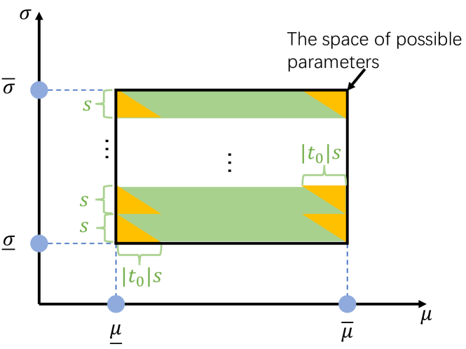
Figure 12: The construction for proof of Proposition 5 for Gaussian distributions. We separate the space of possible parameters into two regions (yellow and green) and bound the attacker’s success rate on each region separately.

In Fig. 12, we separate the space of possible data parameters into two regions represented by yellow and green colors. The yellow regions $S_{yellow}$ constitute right triangles with height $s$ and width $\lvert t_{0}\rvert s$. The green region $S_{green}$ is the rest of the parameter space. The high-level idea of our proof is as follows. Note that for any parameter $\theta\in S_{green}$, there exists a $\mathcal{S}_{\mu,i}$ s.t. $\theta\in\mathcal{S}_{\mu,i}$ and $\mathcal{S}_{\mu,i}\subset S_{green}$. Therefore, we can bound the attack success rate if $\theta\in S_{green}$. At the same time, the probability of $\theta\in S_{yellow}$ is bounded. Therefore, we can bound the overall attacker’s success rate (i.e., $\Pi_{\epsilon,\omega_{\Theta}}$). More specifically, let the optimal attacker be $\hat{g}^{*}$. We have

$$\Pi_{\epsilon,\omega_{\Theta}}{} =\mathbb{P}\left(\hat{g}^{*}\left(\theta^{\prime}\right)\in\left[g\left(\theta\right)-\epsilon,g\left(\theta\right)+\epsilon\right]\right)$$

$$=\int_{\theta\in S_{green}}p(\theta)\mathbb{P}\left(\hat{g}^{*}\left(\theta^{\prime}\right)\in\left[g\left(\theta\right)-\epsilon,g\left(\theta\right)+\epsilon\right]\right)d\theta$$

$$\quad+\int_{\theta\in S_{yellow}}p(\theta)\mathbb{P}\left(\hat{g}^{*}\left(\theta^{\prime}\right)\in\left[g\left(\theta\right)-\epsilon,g\left(\theta\right)+\epsilon\right]\right)d\theta$$

$$<\frac{2\epsilon}{\lvert t_{0}+Q_{\alpha}\rvert s}+\frac{\lvert t_{0}\rvert s}{\overline{\mu}-\underline{\mu}}.$$

For the distortion, it is straightforward to get that $\Delta=\frac{s}{2}\sqrt{\frac{2}{\pi}}e^{-\frac{1}{2}t_{0}^{2}}-\frac{t_{0}s}{2}\left(1-2\Phi\left(t_{0}\right)\right)$ from Eq. 22, and $\Delta_{\text{opt}}>\left(\lceil{\frac{1}{\Pi_{\epsilon,\omega_{\Theta}}{}}}\rceil-1\right)\cdot 2\ratio\epsilon\geq 2\ratio\epsilon$, where is defined in Corollary 4. We can get that $\left(\Pi_{\epsilon,\omega_{\Theta}}-\frac{\lvert t_{0}\rvert s}{\overline{\mu}-\underline{\mu}}\right)\cdot\Delta<2\ratio\epsilon$ and

$$\Delta =\Delta_{\text{opt}}+\Delta-\Delta_{\text{opt}}$$

$$<\Delta_{\text{opt}}+\Delta-\left(\lceil{\frac{1}{\Pi_{\epsilon,\omega_{\Theta}}}}\rceil-1\right)\cdot 2\ratio\epsilon$$

$$\leq\Delta_{\text{opt}}+2\ratio\epsilon+\Delta-{{\frac{2\ratio\epsilon}{\Pi_{\epsilon,\omega_{\Theta}}}}}$$

$$<\Delta_{\text{opt}}+2\ratio\epsilon+\frac{\frac{\lvert t_{0}\rvert s}{\overline{\mu}-\underline{\mu}}}{\frac{2\epsilon}{\lvert t_{0}+Q_{\alpha}\rvert s}+\frac{\lvert t_{0}\rvert s}{\overline{\mu}-\underline{\mu}}}\cdot\Delta$$

$$=\left(1+\frac{\lvert t_{0}\rvert\cdot\lvert t_{0}+Q_{\alpha}\rvert s^{2}}{2\epsilon\left(\overline{\mu}-\underline{\mu}\right)}\right)\left(\Delta_{\text{opt}}+2\ratio\epsilon\right)$$

$$\leq\left(2+\frac{\lvert t_{0}\rvert\cdot\lvert t_{0}+Q_{\alpha}\rvert s^{2}}{\epsilon\left(\overline{\mu}-\underline{\mu}\right)}\right)\Delta_{\text{opt}}.$$

∎

F-B2 Uniform Distribution

Proof.

We first focus on the proof for $\Pi_{\epsilon,\omega_{\Theta}}$.

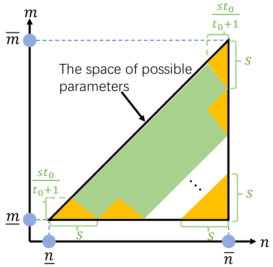
Figure 13: The construction for proof of Proposition 5 for uniform distributions. We separate the space of possible parameters into two regions (yellow and green) and bound the attacker’s success rate on each region separately.

In Fig. 13, we separate the space of possible data parameters into two regions represented by yellow and green colors. The yellow regions $S_{yellow}$ constitute triangles with height $\frac{st_{0}}{t_{0}+1}$ and width $s$ (except for the right-bottom triangle with height and width $s$). The green region $S_{green}$ is the rest of the parameter space. The high-level idea of our proof is as follows. Note that for any parameter $\theta\in S_{green}$, there exists a $\mathcal{S}_{\mu,i}$ s.t. $\theta\in\mathcal{S}_{\mu,i}$ and $\mathcal{S}_{\mu,i}\subset S_{green}$. Therefore, we can bound the attack success rate if $\theta\in S_{green}$. At the same time, the probability of $\theta\in S_{yellow}$ is bounded. Therefore, we can bound the overall attacker’s success rate (i.e., $\Pi_{\epsilon,\omega_{\Theta}}$). More specifically, let the optimal attacker be $\hat{g}^{*}$. We have

$$\Pi_{\epsilon,\omega_{\Theta}}{} =\mathbb{P}\left(\hat{g}^{*}\left(\theta^{\prime}\right)\in\left[g\left(\theta\right)-\epsilon,g\left(\theta\right)+\epsilon\right]\right)$$

$$=\int_{\theta\in S_{green}}p(\theta)\mathbb{P}\left(\hat{g}^{*}\left(\theta^{\prime}\right)\in\left[g\left(\theta\right)-\epsilon,g\left(\theta\right)+\epsilon\right]\right)d\theta$$

$$\quad+\int_{\theta\in S_{yellow}}p(\theta)\mathbb{P}\left(\hat{g}^{*}\left(\theta^{\prime}\right)\in\left[g\left(\theta\right)-\epsilon,g\left(\theta\right)+\epsilon\right]\right)d\theta$$

$$<\frac{2\epsilon\left(t_{0}+1\right)}{\lvert\left(1-\alpha\right)t_{0}-\alpha\rvert s}+\frac{2s\cdot t_{0}}{\left(t_{0}+1\right)\left(\overline{m}-\underline{m}\right)}+\frac{s^{2}}{2\left(\overline{m}-\underline{m}\right)^{2}}.$$

The second term $\frac{2s\cdot t_{0}}{\left(t_{0}+1\right)\left(\overline{m}-\underline{m}\right)}$ bounds the probability of the yellow region except for the right-bottom triangle, and the last term $\frac{s^{2}}{2\left(\overline{m}-\underline{m}\right)^{2}}$ is the probability of the right-bottom triangle.

For the distortion, it is straightforward to get that $\Delta=\frac{\left(t_{0}^{2}+1\right)s}{4(t_{0}+1)^{2}}$ from Eq. 23, and $\Delta_{\text{opt}}>\left(\lceil{\frac{1}{\Pi_{\epsilon,\omega_{\Theta}}{}}}\rceil-1\right)\cdot 2\ratio\epsilon\geq 2\ratio\epsilon$, where is defined in Corollary 4. We can get that $\left(\Pi_{\epsilon,\omega_{\Theta}}-\frac{2s\cdot t_{0}}{\left(t_{0}+1\right)\left(\overline{m}-\underline{m}\right)}-\frac{s^{2}}{2\left(\overline{m}-\underline{m}\right)^{2}}\right)\cdot\Delta<2\ratio\epsilon$ and

$$\Delta=\Delta_{\text{opt}}+\Delta-\Delta_{\text{opt}}$$

$$<\Delta_{\text{opt}}+\Delta-\left(\lceil{\frac{1}{\Pi_{\epsilon,\omega_{\Theta}}}}\rceil-1\right)\cdot 2\ratio\epsilon$$

$$\leq\Delta_{\text{opt}}+2\ratio\epsilon+\Delta-{{\frac{2\ratio\epsilon}{\Pi_{\epsilon,\omega_{\Theta}}}}}$$

$$<\Delta_{\text{opt}}+2\ratio\epsilon+\frac{\frac{2s\cdot t_{0}}{\left(t_{0}+1\right)\left(\overline{m}-\underline{m}\right)}+\frac{s^{2}}{2\left(\overline{m}-\underline{m}\right)^{2}}}{\frac{2\epsilon\left(t_{0}+1\right)}{\lvert\left(1-\alpha\right)t_{0}-\alpha\rvert s}+\frac{2s\cdot t_{0}}{\left(t_{0}+1\right)\left(\overline{m}-\underline{m}\right)}+\frac{s^{2}}{2\left(\overline{m}-\underline{m}\right)^{2}}}\cdot\Delta$$

$$=\left(1+\frac{\lvert\left(1-\alpha\right)t_{0}-\alpha\rvert s}{2\epsilon\left(t_{0}+1\right)}\left(\frac{2s\cdot t_{0}}{\left(t_{0}+1\right)\left(\overline{m}-\underline{m}\right)}+\frac{s^{2}}{2\left(\overline{m}-\underline{m}\right)^{2}}\right)\right)\left(\Delta_{\text{opt}}+2\ratio\epsilon\right)$$

$$\leq\left(2+\frac{\lvert\left(1-\alpha\right)t_{0}-\alpha\rvert s}{\epsilon\left(t_{0}+1\right)}\cdot\left(\frac{2s\cdot t_{0}}{\left(t_{0}+1\right)\left(\overline{m}-\underline{m}\right)}+\frac{s^{2}}{2\left(\overline{m}-\underline{m}\right)^{2}}\right)\right)\Delta_{\text{opt}}.$$

When ${\frac{s^{2}}{\overline{m}-\underline{m}}}\rightarrow 0$ as $s,(\overline{m}-\underline{m})\to\infty$, we can get that ${\frac{s^{3}}{\left(\overline{m}-\underline{m}\right)^{2}}}\rightarrow 0$. Therefore, in this case, $\lim{\sup_{{\frac{s^{2}}{\overline{m}-\underline{m}}}\rightarrow 0}}\Delta<3\Delta_{\text{opt}}$.

∎

F-C Privacy-Distortion Performance of Mechanism 3 with Relaxed Assumption

For Gaussian distribution, we relax Assumption 5 as follows.

Assumption 6.

The prior over Gaussian distribution parameters satisfies $\text{Supp}\left({\text{\textmugreek},\text{\textsigma{}}}\right)=\left\{(a,b)|a\in\left[\underline{\mu},\overline{\mu}\right),b\in\left[\underline{\sigma},\overline{\sigma}\right)\right\}$, $f_{\text{\textmugreek},\text{\textsigma{}}}\left(a,b\right)=f_{\text{\textmugreek}}\left(a\right)\cdot f_{\text{\textsigma{}}}\left(b\right)$, and $f_{\text{\textmugreek}}\left(a\right)$ (resp. $f_{\text{\textsigma{}}}\left(b\right)$) is $\mathcal{L}_{\mu}$-Lipschitz (resp. $\mathcal{L}_{\sigma}$-Lipschitz) and has lower bound $\frac{k_{\mu}}{\overline{\mu}-\underline{\mu}}$ with $k_{\mu}\in(0,1]$ (resp. $\frac{k_{\sigma}}{\overline{\sigma}-\underline{\sigma}}$ with $k_{\sigma}\in(0,1]$).

Based on Assumption 6, the Privacy-distortion performance of Mechanism 3 is shown below.

Proposition 6.

Under Assumption 6, Mechanism 3 has the following $\Delta$ and $\Pi_{\epsilon,\omega_{\Theta}}{}$ value/bound:

$$\Delta =\frac{s}{2}\sqrt{\frac{2}{\pi}}e^{-\frac{1}{2}t_{0}^{2}}-\frac{t_{0}s}{2}\left(1-2\Phi\left(t_{0}\right)\right),$$

$$\Pi_{\epsilon,\omega_{\Theta}} <\frac{\frac{2\epsilon}{\lvert t_{0}+Q_{\alpha}\rvert}\cdot\left[\underline{c}+\mathcal{L}_{\mu,\sigma}\left(\frac{s}{2}-t^{*}-\frac{\epsilon}{\lvert t_{0}+Q_{\alpha}\rvert}\right)\right]}{\underline{c}s+\frac{\mathcal{L}_{\mu,\sigma}}{2}\left(\frac{s}{2}-t^{*}\right)^{2}}+$$

$$M\left(\overline{\mu}-\underline{\mu},\frac{k_{\mu}}{\overline{\mu}-\underline{\mu}},\mathcal{L}_{\mu},1\right)\cdot M\left(\overline{\sigma}-\underline{\sigma},\frac{k_{\sigma}}{\overline{\sigma}-\underline{\sigma}},\mathcal{L}_{\sigma},1\right)\cdot\left(\overline{\sigma}-\underline{\sigma}\right)\lvert t_{0}\rvert s,$$

where $\underline{c}=\frac{k_{\mu}k_{\sigma}}{\left(\overline{\mu}-\underline{\mu}\right)\cdot\left(\overline{\sigma}-\underline{\sigma}\right)}$, function $M$ satisfies

$$M\left(x,c,\mathcal{L},\mathcal{A}\right)=\begin{cases}\frac{\mathcal{A}}{x}+\frac{\mathcal{L}x}{2},&\text{if }c\leq\frac{\mathcal{A}}{x}-\frac{\mathcal{L}x}{2}\\ c+\sqrt{2\mathcal{L}\left(\mathcal{A}-cx\right)},&\text{if }c>\frac{\mathcal{A}}{x}-\frac{\mathcal{L}x}{2}\end{cases},$$

$\mathcal{L}_{\mu,\sigma}=\mathcal{L}_{\sigma}\cdot M\left(\frac{\overline{\mu}-\underline{\mu}}{\lvert t_{0}\rvert},\frac{k_{\mu}}{\overline{\mu}-\underline{\mu}},\lvert t_{0}\rvert\mathcal{L}_{\mu},\frac{1}{\lvert t_{0}\rvert}\right)+\lvert t_{0}\rvert\mathcal{L}_{\mu}\cdot M\left(\overline{\sigma}-\underline{\sigma},\frac{k_{\sigma}}{\overline{\sigma}-\underline{\sigma}},\mathcal{L}_{\sigma},1\right)$, and $t^{*}=\frac{s}{2}+\frac{\underline{c}}{\mathcal{L}_{\mu,\sigma}}-\frac{\epsilon}{\lvert t_{0}+Q_{\alpha}\rvert}-\sqrt{\left(\frac{\underline{c}}{\mathcal{L}_{\mu,\sigma}}-\frac{\epsilon}{\lvert t_{0}+Q_{\alpha}\rvert}\right)^{2}+\frac{2\underline{c}s}{\mathcal{L}_{\mu,\sigma}}}$.

Proof.

It is straightforward to get the formula for $\Delta$ from Eq. 22. Here we focus on the proof for $\Pi_{\epsilon,\omega_{\Theta}}$.

Similar to § D-B2, based on Lemma 1 and Lemma 2, we can get that

$$\sup_{\theta\in S_{green}}\mathbb{P}\left(\hat{g}^{*}\left(\theta^{\prime}\right)\in\left[g\left(\theta\right)-\epsilon,g\left(\theta\right)+\epsilon\right]\right)$$

$$=\sup_{i\in\mathbb{N},\mu,t^{\prime}\in\mathbb{R}}\frac{\int_{\max\left\{-\frac{s}{2},t^{\prime}\right\}}^{\min\left\{\frac{s}{2},t^{\prime}+\frac{2\epsilon}{\lvert t_{0}+Q_{\alpha}\rvert}\right\}}f_{\text{\textmugreek},\text{\textsigma{}}}\left(\mu+t_{0}\cdot t,\underline{\sigma}+\left(i+0.5\right)\cdot s+t\right)\mathrm{d}t}{\int_{-\frac{s}{2}}^{\frac{s}{2}}f_{\text{\textmugreek},\text{\textsigma{}}}\left(\mu+t_{0}\cdot t,\underline{\sigma}+\left(i+0.5\right)\cdot s+t\right)\mathrm{d}t}$$

$$\leq\frac{\frac{2\epsilon}{\lvert t_{0}+Q_{\alpha}\rvert}\cdot\left[\underline{c}+\mathcal{L}_{\mu,\sigma}\left(\frac{s}{2}-t^{*}-\frac{\epsilon}{\lvert t_{0}+Q_{\alpha}\rvert}\right)\right]}{\underline{c}s+\frac{\mathcal{L}_{\mu,\sigma}}{2}\left(\frac{s}{2}-t^{*}\right)^{2}},$$

where $t^{*}=\frac{s}{2}+\frac{\underline{c}}{\mathcal{L}_{\mu,\sigma}}-\frac{\epsilon}{\lvert t_{0}+Q_{\alpha}\rvert}-\sqrt{\left(\frac{\underline{c}}{\mathcal{L}_{\mu,\sigma}}-\frac{\epsilon}{\lvert t_{0}+Q_{\alpha}\rvert}\right)^{2}+\frac{2\underline{c}s}{\mathcal{L}_{\mu,\sigma}}}$, $\mathcal{L}_{\mu,\sigma}=\mathcal{L}_{\sigma}\cdot M\left(\frac{\overline{\mu}-\underline{\mu}}{\lvert t_{0}\rvert},\frac{k_{\mu}}{\overline{\mu}-\underline{\mu}},\lvert t_{0}\rvert\mathcal{L}_{\mu},\frac{1}{\lvert t_{0}\rvert}\right)+\lvert t_{0}\rvert\mathcal{L}_{\mu}\cdot M\left(\overline{\sigma}-\underline{\sigma},\frac{k_{\sigma}}{\overline{\sigma}-\underline{\sigma}},\mathcal{L}_{\sigma},1\right)$, and $\underline{c}=\frac{k_{\mu}k_{\sigma}}{\left(\overline{\mu}-\underline{\mu}\right)\cdot\left(\overline{\sigma}-\underline{\sigma}\right)}$.

As for $\int_{\theta\in S_{yellow}}p(\theta)d\theta$, we have

$$\int_{\theta\in S_{yellow}}p(\theta)d\theta$$

$$\leq M\left(\overline{\mu}-\underline{\mu},\frac{k_{\mu}}{\overline{\mu}-\underline{\mu}},\mathcal{L}_{\mu},1\right)\cdot M\left(\overline{\sigma}-\underline{\sigma},\frac{k_{\sigma}}{\overline{\sigma}-\underline{\sigma}},\mathcal{L}_{\sigma},1\right)\cdot\int_{\theta\in S_{yellow}}d\theta$$

$$=M\left(\overline{\mu}-\underline{\mu},\frac{k_{\mu}}{\overline{\mu}-\underline{\mu}},\mathcal{L}_{\mu},1\right)\cdot M\left(\overline{\sigma}-\underline{\sigma},\frac{k_{\sigma}}{\overline{\sigma}-\underline{\sigma}},\mathcal{L}_{\sigma},1\right)\cdot\left(\overline{\sigma}-\underline{\sigma}\right)\lvert t_{0}\rvert s.$$

Above all, we can get that

$$\Pi_{\epsilon,\omega_{\Theta}}{} <\sup_{\theta\in S_{green}}\mathbb{P}\left(\hat{g}^{*}\left(\theta^{\prime}\right)\in\left[g\left(\theta\right)-\epsilon,g\left(\theta\right)+\epsilon\right]\right)+\int_{\theta\in S_{yellow}}p(\theta)d\theta.$$

$$\leq\frac{\frac{2\epsilon}{\lvert t_{0}+Q_{\alpha}\rvert}\cdot\left[\underline{c}+\mathcal{L}_{\mu,\sigma}\left(\frac{s}{2}-t^{*}-\frac{\epsilon}{\lvert t_{0}+Q_{\alpha}\rvert}\right)\right]}{\underline{c}s+\frac{\mathcal{L}_{\mu,\sigma}}{2}\left(\frac{s}{2}-t^{*}\right)^{2}}+$$

$$M\left(\overline{\mu}-\underline{\mu},\frac{k_{\mu}}{\overline{\mu}-\underline{\mu}},\mathcal{L}_{\mu},1\right)\cdot M\left(\overline{\sigma}-\underline{\sigma},\frac{k_{\sigma}}{\overline{\sigma}-\underline{\sigma}},\mathcal{L}_{\sigma},1\right)\cdot\left(\overline{\sigma}-\underline{\sigma}\right)\lvert t_{0}\rvert s,$$

where $M(\cdot,\cdot,\cdot,\cdot),\underline{c},\mathcal{L}_{\mu,\sigma},t^{*}$ are defined as above. ∎

Appendix G Case Study with Secret = Standard Deviation

In this section, we discuss how to protect standard deviation for several continuous and discrete distributions.

G-A Continuous Distributions

We consider the same distributions discussed in § VI-B and Appendix F: Gaussian, uniform, and (shifted) exponential distributions.

Corollary 5 (Privacy lower bound, secret = standard deviation of a continuous distribution).

Consider the secret function $g\left(\theta\right)=$ standard deviation of $f_{X_{\theta}}$. For any $T\in\left(0,1\right)$, when $\Pi_{\epsilon,\omega_{\Theta}}\leq T$, we have $\Delta>\left(\lceil{\frac{1}{T}}\rceil-1\right)\cdot 2\ratio\epsilon$, where the value of depends on the type of the distributions:

• Gaussian:

  $$\ratio=\min_{t}\sqrt{\frac{1}{2\pi}}e^{-\frac{1}{2}t^{2}}-t\left(\frac{1}{2}-\Phi\left(t\right)\right),$$

  where $\Phi$ denotes the CDF of the standard Gaussian distribution.

• Uniform: $\ratio=\frac{\sqrt{3}}{4}.$

• Exponential: $\ratio=\frac{1}{2}.$

• Shifted exponential: $\ratio=\frac{\ln{2}}{2}.$

The proof is in § G-C. The bounds for Gaussian can be computed numerically, while the bounds for all other distributions are in closed form.

Next, we present the data release mechanism for these distributions and the secret under the same assumption as Assumption 2.

Mechanism 4 (For secret = standard deviation of a continuous distribution).

We design mechanisms for each of the distributions.

• Gaussian:

  $$\mathcal{S}_{\mu,i} =\left\{\left(\mu+t_{0}\cdot t,\underline{\sigma}+\left(i+0.5\right)\cdot s+t\right)|t\in\left[-\frac{s}{2},\frac{s}{2}\right)\right\}~{}~{},$$

  $$\theta^{*}_{\mu,i} =\left(\mu,\underline{\sigma}+\left(i+0.5\right)\cdot s\right)~{}~{},$$

  $$\mathcal{I} =\left\{\left(\mu,i\right)|i\in\mathbb{N},\mu\in\mathbb{R}\right\},$$

  where $s$ is a hyper-parameter of the mechanism that divides $\left(\overline{\sigma}-\underline{\sigma}\right)$ and

  $$t_{0}=\arg\min_{t}\sqrt{\frac{1}{2\pi}}e^{-\frac{1}{2}t^{2}}-t\left(\frac{1}{2}-\Phi\left(t\right)\right).$$

  .

• Uniform:

  $$\mathcal{S}_{m,i} =\scalebox{0.8}{$\left\{\left(m-t,m+\left(i+0.5\right)\cdot s+t\right)|t\in\left(-\frac{s}{4},\frac{s}{4}\right]\right\}$}~{}~{},$$

  $$\theta^{*}_{m,i} =\left(m,m+\left(i+0.5\right)\cdot s\right)~{}~{},$$

  $$\mathcal{I} =\left\{\left(m,i\right)|i\in\mathbb{Z}_{>0},m\in\mathbb{R}\right\},$$

  where $s>0$ is a hyper-parameter of the mechanism that divides $\left(\overline{m}-\underline{m}\right)$.

• Exponential:

  $$\mathcal{S}_{i} =\left[\underline{\lambda}+i\cdot s,\underline{\lambda}+\left(i+1\right)\cdot s\right)~{}~{},$$

  $$\theta^{*}_{i} =\underline{\lambda}+\left(i+0.5\right)\cdot s~{}~{},$$

  $$\mathcal{I} =\mathbb{N},$$

  where $s>0$ is a hyper-parameter of the mechanism that divides $\left(\overline{\lambda}-\underline{\lambda}\right)$.

• Shifted exponential:

  $$\mathcal{S}_{i,h} =\left\{\left(\underline{\lambda}+\left(i+0.5\right)s+t,h-\ln 2\cdot t\right)|t\in\left[-\frac{s}{2},\frac{s}{2}\right)\right\}~{}~{},$$

  $$\theta^{*}_{i,h} =\left(\underline{\lambda}+\left(i+0.5\right)s,h\right)~{}~{},$$

  $$\mathcal{I} =\left\{(i,h)|i\in\mathbb{N},h\in\mathbb{R}\right\},$$

  where $s>0$ is a hyper-parameter of the mechanism that divides $\left(\overline{\lambda}-\underline{\lambda}\right)$.

These data release mechanisms achieve the following $\Delta$ and $\Pi_{\epsilon,\omega_{\Theta}}$.

Proposition 7.

Under Assumption 2, Mechanism 4 has the following $\Delta$ and $\Pi_{\epsilon,\omega_{\Theta}}{}$ value/bound.

• Gaussian:

  $$\Pi_{\epsilon,\omega_{\Theta}} <\frac{2\epsilon}{s}+\frac{\lvert t_{0}\rvert s}{\overline{\mu}-\underline{\mu}},$$

  $$\Delta =\frac{s}{2}\sqrt{\frac{2}{\pi}}e^{-\frac{1}{2}t_{0}^{2}}-\frac{t_{0}s}{2}\left(1-2\Phi\left(t_{0}\right)\right)<\left(2+\frac{\lvert t_{0}\rvert s^{2}}{\left(\overline{\mu}-\underline{\mu}\right)\epsilon}\right)\Delta_{\text{opt}},$$

  where $t_{0}$ is defined in Mechanism 4. Under the “high-precision” regime where ${\frac{s^{2}}{\overline{\mu}-\underline{\mu}}}\rightarrow 0$ as $s,(\overline{\mu}-\underline{\mu})\to\infty$, $\Delta$ satisfies

  $$\lim{\sup_{{\frac{s^{2}}{\overline{\mu}-\underline{\mu}}}\rightarrow 0}}\Delta<3\Delta_{\text{opt}}.$$

• Uniform:

  $$\Pi_{\epsilon,\omega_{\Theta}} <\frac{4\sqrt{3}\epsilon}{s}+\frac{s}{\left(\overline{m}-\underline{m}\right)}+\frac{s^{2}}{2\left(\overline{m}-\underline{m}\right)^{2}},$$

  $$\Delta =\frac{s}{8}<\left(2+\frac{s}{2\sqrt{3}\epsilon}\cdot\left(\frac{s}{{\overline{m}-\underline{m}}}+\frac{s^{2}}{2\left(\overline{m}-\underline{m}\right)^{2}}\right)\right)\Delta_{\text{opt}}.$$

  Under the “high-precision” regime where ${\frac{s^{2}}{\overline{m}-\underline{m}}}\rightarrow 0$ as $s,(\overline{m}-\underline{m})\to\infty$, $\Delta$ satisfies

  $$\lim{\sup_{{\frac{s^{2}}{\overline{m}-\underline{m}}}\rightarrow 0}}\Delta<3\Delta_{\text{opt}}.$$

• Exponential:

  $$\Pi_{\epsilon,\omega_{\Theta}} =\frac{2\epsilon}{s},$$

  $$\Delta =\frac{1}{2}s<2\Delta_{\text{opt}}.$$

• Shifted exponential:

  $$\Pi_{\epsilon,\omega_{\Theta}} <\frac{2\epsilon}{s}+\frac{s\ln 2}{\overline{h}-\underline{h}},$$

  $$\Delta =\frac{s\ln 2}{2}<\left(2+\frac{s^{2}\ln 2}{\epsilon\left(\overline{h}-\underline{h}\right)}\right)\Delta_{\text{opt}}.$$

  Under the “high-precision” regime where ${\frac{s^{2}}{\overline{h}-\underline{h}}}\rightarrow 0$ as $s,(\overline{h}-\underline{h})\to\infty$, $\Delta$ satisfies

  $$\lim{\sup_{{\frac{s^{2}}{\overline{h}-\underline{h}}}\rightarrow 0}}\Delta<3\Delta_{\text{opt}}.$$

The proof is in § G-D. For Gaussian, exponential and shifted exponential distributions, we relax Assumption 2 and analyze the privacy-distortion performance of Mechanism 4 in § G-E. From these propositions, we have similar takeaways as the alpha-quantile case ( § VI-B): (1) data holder can use $s$ to control the trade-off between distortion and privacy, and (2) the mechanism is order-optimal under the “high-precision” regime.

G-B Discrete Distributions

Here, we consider the same discrete distributions studied in Appendix E: Geometric distributions, binomial distributions, and Poisson distributions. We first analyze the lower bound.

Corollary 6 (Privacy lower bound, secret = standard deviation of a discrete distribution).

Consider the secret function $g\left(\theta\right)=$ standard deviation of $f_{X_{\theta}}$. For any $T\in\left(0,1\right)$, when $\Pi_{\epsilon,\omega_{\Theta}}\leq T$, we have $\Delta>\left(\lceil{\frac{1}{T}}\rceil-1\right)\cdot 2\ratio\epsilon$, where the value of depends on the type of the distributions:

• Geometric:

  $$\ratio=\inf_{\underline{\theta}<\theta_{1}<\theta_{2}\leq\overline{\theta}}\frac{\left(1-\theta_{2}\right)^{h\left(\theta_{1},\theta_{2}\right)}-\left(1-\theta_{1}\right)^{h\left(\theta_{1},\theta_{2}\right)}}{2\left(\frac{\sqrt{1-\theta_{2}}}{\theta_{2}}-\frac{\sqrt{1-\theta_{1}}}{\theta_{1}}\right)}~{}~{},$$

  where $h\left(\theta_{1},\theta_{2}\right)=\lfloor{\frac{\log\left(\theta_{2}\right)-\log\left(\theta_{1}\right)}{\log\left(1-\theta_{1}\right)-\log\left(1-\theta_{2}\right)}}\rfloor+1$.

• Binomial:

  $$\ratio=\inf_{\underline{\theta}<\theta_{1}<\theta_{2}\leq\overline{\theta}}$$

  where $h\left(\theta_{1},\theta_{2}\right)=\lfloor{k^{\prime}}\rfloor$, $k^{\prime}=n\ln\left(\frac{1-\theta_{2}}{1-\theta_{1}}\right)\Big{/}\ln\left({\frac{\theta_{1}\left(1-\theta_{2}\right)}{\theta_{2}\left(1-\theta_{1}\right)}}\right)$, and $I$ represents the regularized incomplete beta function.

• Poisson:

  $$\ratio=\inf_{\underline{\theta}<\theta_{1}<\theta_{2}\leq\overline{\theta}}\frac{Q\left(h\left(\theta_{1},\theta_{2}\right),\theta_{2}\right)-Q\left(h\left(\theta_{1},\theta_{2}\right),\theta_{1}\right)}{2\left(\sqrt{\theta_{1}}-\sqrt{\theta_{2}}\right)},$$

  where $h\left(\theta_{1},\theta_{2}\right)=\lfloor{\frac{\theta_{1}-\theta_{2}}{\ln\left(\theta_{1}\right)-\ln\left(\theta_{2}\right)}}\rfloor+1$ and $Q$ is the regularized gamma function.

The proof is in § G-F. The above lower bounds can be computed numerically.

Since these distributions only have one parameter, we can use Algorithm 1 and Algorithm 3 to derive a data release mechanism. The performance of greedy-based and dynamic-programming-based data release mechanisms for each distribution is shown in Fig. 14.

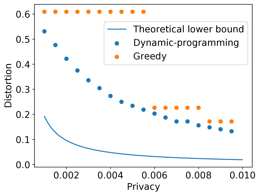
(a) Distribution = Geometric

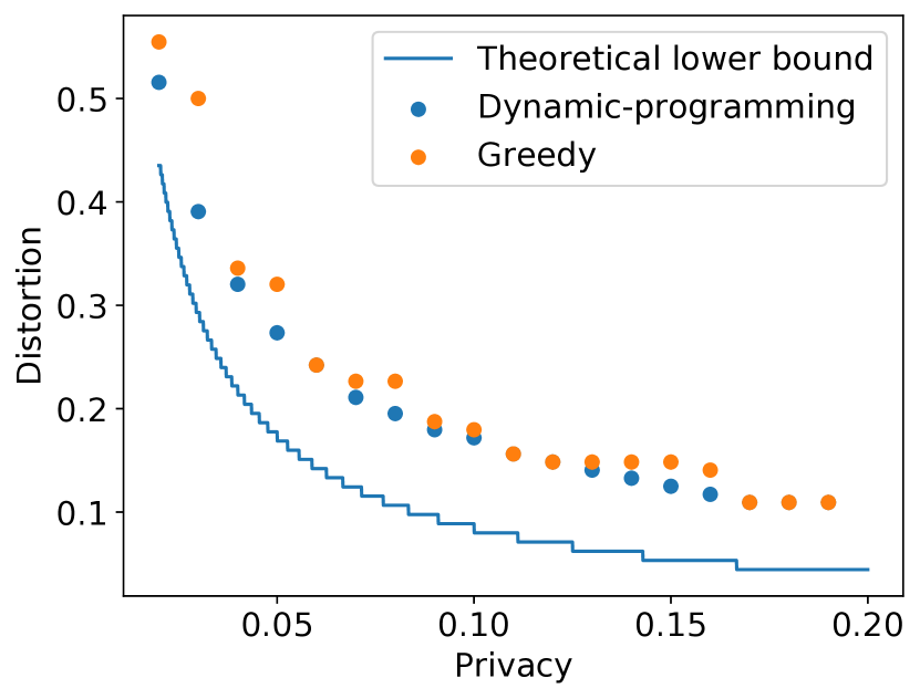
(b) Distribution = Binomial

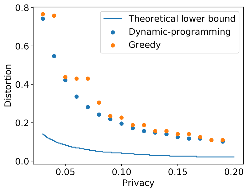
(c) Distribution = Poisson

Figure 14: Privacy-distortion performance of Algorithm 1 and Algorithm 3 for binomial and Poisson distribution when secret = standard deviation.

G-C Proof of Corollary 5

G-C1 Gaussian Distribution

Proof.

Let $X_{\mu_{1},\sigma_{2}},X_{\mu_{2},\sigma_{2}}$ be two Gaussian random variables with means $\mu_{1},\mu_{2}$ and sigmas $\sigma_{1},\sigma_{2}$ respectively, where $\sigma_{1}\not=\sigma_{2}$. Let $\Phi$ denotes the CDF of the standard Gaussian distribution. We can get that

$$D\left(X_{\mu_{1},\sigma_{1}},X_{\mu_{2},\sigma_{2}}\right) =\left(\mu_{1}-\mu_{2}\right)\left(\Phi\left(\frac{\mu_{1}-\mu_{2}}{\sigma_{2}-\sigma_{1}}\right)-\frac{1}{2}\right)$$

$$\quad+\sqrt{\frac{1}{2\pi}}\left(\sigma_{2}-\sigma_{1}\right)e^{-\frac{1}{2}\left(\frac{\mu_{1}-\mu_{2}}{\sigma_{2}-\sigma_{1}}\right)^{2}},$$

$$R\left(X_{\mu_{1},\sigma_{1}},X_{\mu_{2},\sigma_{2}}\right) =\lvert\sigma_{1}-\sigma_{2}\rvert.$$

Let $\frac{\mu_{1}-\mu_{2}}{\sigma_{1}-\sigma_{2}}\triangleq t$, we can get that

$$\frac{D\left(X_{\mu_{1},\sigma_{1}},X_{\mu_{2},\sigma_{2}}\right)}{R\left(X_{\mu_{1},\sigma_{1}},X_{\mu_{2},\sigma_{2}}\right)} =\sqrt{\frac{1}{2\pi}}e^{-\frac{1}{2}t^{2}}-t\left(\frac{1}{2}-\Phi\left(t\right)\right)\triangleq h\left(t\right).$$

Therefore we can get that

$$\ratio=\min_{t}h\left(t\right).$$

∎

G-C2 Uniform Distribution

Proof.

Let $X_{m_{1},n_{1}},X_{m_{2},n_{2}}$ be two uniform random variables. Let $F_{X_{m_{1},n_{1}}},F_{X_{m_{2},n_{2}}}$ be their CDFs, and let $m_{2}\geq m_{1}$ without loss of generality. We can get that

$$D\left(X_{m_{1},n_{1}},X_{m_{2},n_{2}}\right) =\frac{1}{2}d_{\text{Wasserstein-1}}\left(\omega_{X_{m_{1},n_{1}}}\|\omega_{X_{m_{2},n_{2}}}\right)$$

$$=\frac{1}{2}\int_{-\infty}^{+\infty}\lvert F_{X_{m_{1},n_{1}}}\left(x\right)-F_{X_{m_{2},n_{2}}}\left(x\right)\rvert\mathrm{d}x$$

$$=\begin{cases}\frac{m_{2}-m_{1}+n_{2}-n_{1}}{4}&n_{2}\geq n_{1}\\ \frac{\left(m_{2}-m_{1}\right)^{2}+\left(n_{1}-n_{2}\right)^{2}}{4\left(m_{2}-m_{1}+\left(n_{1}-n_{2}\right)\right)}&n_{2}<n_{1}\end{cases},$$

$$R\left(X_{m_{1},n_{1}},X_{m_{2},n_{2}}\right) =\left|\frac{1}{\sqrt{12}}\left(n_{1}-m_{1}\right)-\frac{1}{\sqrt{12}}\left(n_{2}-m_{2}\right)\right|$$

$$=\frac{1}{\sqrt{12}}\lvert m_{2}-m_{1}-\left(n_{2}-n_{1}\right)\rvert.$$

Therefore, we can get that when $n_{2}\geq n_{1}$, we have

$$\frac{D\left(X_{m_{1},n_{1}},X_{m_{2},n_{2}}\right)}{R\left(X_{m_{1},n_{1}},X_{m_{2},n_{2}}\right)} =\frac{\sqrt{3}}{2}\frac{m_{2}-m_{1}+n_{2}-n_{1}}{\lvert m_{2}-m_{1}-\left(n_{2}-n_{1}\right)\rvert}$$

$$\geq\frac{\sqrt{3}}{2}.$$

When $n_{2}<n_{1}$, we have

$$\frac{D\left(X_{m_{1},n_{1}},X_{m_{2},n_{2}}\right)}{R\left(X_{m_{1},n_{1}},X_{m_{2},n_{2}}\right)}=\frac{\sqrt{3}}{2}\frac{\left(m_{2}-m_{1}\right)^{2}+\left(n_{1}-n_{2}\right)^{2}}{\left(m_{2}-m_{1}+\left(n_{1}-n_{2}\right)\right)^{2}}$$

$$\quad=\frac{\sqrt{3}}{2}\frac{\left(m_{2}-m_{1}\right)^{2}+\left(n_{1}-n_{2}\right)^{2}}{\left(m_{2}-m_{1}\right)^{2}+\left(n_{1}-n_{2}\right)^{2}+2\left(m_{2}-m_{1}\right)\left(n_{1}-n_{2}\right)}$$

$$\quad\geq\frac{\sqrt{3}}{2}\cdot\frac{\left(m_{2}-m_{1}\right)^{2}+\left(n_{1}-n_{2}\right)^{2}}{2\left[\left(m_{2}-m_{1}\right)^{2}+\left(n_{1}-n_{2}\right)^{2}\right]}$$

$$\quad=\frac{\sqrt{3}}{4}.$$

Therefore we can get that

$$\ratio=\frac{\sqrt{3}}{4}.$$

∎

G-C3 Exponential Distribution

Proof.

Let $X_{\lambda_{1}},X_{\lambda_{2}}$ be two exponential random variables. We have

$$\frac{D\left(X_{\lambda_{1}},X_{\lambda_{2}}\right)}{R\left(X_{\lambda_{1}},X_{\lambda_{2}}\right)} =\frac{\frac{1}{\lambda_{1}}-\frac{1}{\lambda_{2}}}{2\left(\frac{1}{\lambda_{1}}-\frac{1}{\lambda_{2}}\right)}=\frac{1}{2}.$$

Therefore we can get that

$$\ratio=\frac{1}{2}.$$

∎

G-C4 Shifted Exponential Distribution

Proof.

Let $X_{\lambda_{1},h_{1}},X_{\lambda_{2},h_{2}}$ be random variables from shifted exponential distributions. Let $\lambda_{2}\leq\lambda_{1}$ without loss of generality. Let $a=\frac{\lambda_{1}}{\lambda_{2}}$ and $b=\left(h_{1}/\lambda_{1}-h_{2}/\lambda_{2}\right){\lambda_{2}}$. We can get that $f_{X_{\lambda_{1},h_{1}}}\left(x\right)=af_{X_{\lambda_{2},h_{2}}}\left(a\left(x+b\right)\right)$, and

$$D\left(X_{\lambda_{1},h_{1}},X_{\lambda_{2},h_{2}}\right)=\frac{1}{2}d_{\text{Wasserstein-1}}\left(\omega_{X_{\lambda_{1},h_{1}}}\|\omega_{X_{\lambda_{2},h_{2}}}\right)$$

$$=\frac{1}{2}\int_{h_{1}}^{+\infty}\left|x-\left(\frac{x}{a}-b\right)\right|f_{X_{\lambda_{1},h_{1}}}\left(x\right)\mathrm{d}x$$

$$=\frac{\lambda_{2}}{2\lambda_{1}}\int_{h_{1}}^{+\infty}\left|\left(1/\lambda_{2}-1/\lambda_{1}\right)x+h_{1}/\lambda_{1}-h_{2}/\lambda_{2}\right|e^{-\frac{1}{\lambda_{1}}\left(x-h_{1}\right)}\mathrm{d}x$$

$$=\begin{cases}\frac{1}{2}\left(h_{2}-h_{1}+{\lambda_{2}}-{\lambda_{1}}\right)-e^{\frac{h_{2}-h_{1}}{{\lambda_{2}}-{\lambda_{1}}}}\left({\lambda_{2}}-{\lambda_{1}}\right)&\left(h_{1}<h_{2}\right)\\ \frac{1}{2}\left(h_{1}-h_{2}+{\lambda_{1}}-{\lambda_{2}}\right)&\left(h_{1}\geq h_{2}\right)\end{cases},$$

$$R\left(X_{\lambda_{1},h_{1}},X_{\lambda_{2},h_{2}}\right)={\lambda_{1}}-{\lambda_{2}}.$$ (24)

When $\lambda_{1}=\lambda_{2}$ and $h_{1}\not=h_{2}$, we have $\frac{D\left(X_{\lambda_{1},h_{1}},X_{\lambda_{2},h_{2}}\right)}{R\left(X_{\lambda_{1},h_{1}},X_{\lambda_{2},h_{2}}\right)}=\infty$.

When $\lambda_{1}\not=\lambda_{2}$ and $h_{1}<h_{2}$, let $t=\frac{h_{2}-h_{1}}{{\lambda_{1}}-{\lambda_{2}}}\in(0,+\infty)$. We have

$$\frac{D\left(X_{\lambda_{1},h_{1}},X_{\lambda_{2},h_{2}}\right)}{R\left(X_{\lambda_{1},h_{1}},X_{\lambda_{2},h_{2}}\right)} =\frac{h_{2}-h_{1}+{\lambda_{2}}-{\lambda_{1}}-2e^{\frac{h_{2}-h_{1}}{{\lambda_{2}}-{\lambda_{1}}}}\left({\lambda_{2}}-{\lambda_{1}}\right)}{2\left({\lambda_{1}}-{\lambda_{2}}\right)}$$

$$=\frac{t+2e^{-t}-1}{2}$$

$$\geq\frac{\ln 2}{2}.$$

“$=$” achieves when $t=t_{0}=\ln 2$.

When $\lambda_{1}\not=\lambda_{2}$ and $h_{1}\geq h_{2}$, we have

$$\frac{D\left(X_{\lambda_{1},h_{1}},X_{\lambda_{2},h_{2}}\right)}{R\left(X_{\lambda_{1},h_{1}},X_{\lambda_{2},h_{2}}\right)} =\frac{h_{1}-h_{2}+{\lambda_{1}}-{\lambda_{2}}}{2\left({\lambda_{1}}-{\lambda_{2}}\right)}\geq\frac{{\lambda_{1}}-{\lambda_{2}}}{2\left({\lambda_{1}}-{\lambda_{2}}\right)}=\frac{1}{2}.$$

Therefore we can get that

$$\ratio=\frac{\ln 2}{2}.$$

∎

G-D Proof of Proposition 7

The proof outline is almost the same as the ones in § C-D and § F-B. We omit the details and point to the proof sections where we can adapt from.

G-D1 Gaussian Distribution

The proof is the same as § F-B1, except that we use the $D\left(\cdot,\cdot\right)$ and $R\left(\cdot,\cdot\right)$ from § G-C1.

G-D2 Uniform Distribution

The proof is the same as § F-B2, except that we use the $D\left(\cdot,\cdot\right)$ and $R\left(\cdot,\cdot\right)$ from § G-C2.

G-D3 Exponential Distribution

The proof is the same as § C-D1, except that we use the $D\left(\cdot,\cdot\right)$ and $R\left(\cdot,\cdot\right)$ from § G-C3.

G-D4 Shifted Exponential Distribution

The proof is the same as § C-D2, except that we use the $D\left(\cdot,\cdot\right)$ and $R\left(\cdot,\cdot\right)$ from § G-C4.

G-E Privacy-Distortion Performance of Mechanism 4 with Relaxed Assumption

Based on Assumption 6 and Assumption 4, the Privacy-distortion performance of Mechanism 4 is shown below.

Proposition 8.

Under Assumption 6 and Assumption 4, Mechanism 4 has the following $\Delta$ and $\Pi_{\epsilon,\omega_{\Theta}}{}$ value/bound.

• Gaussian:

  $$\Delta =\frac{s}{2}\sqrt{\frac{2}{\pi}}e^{-\frac{1}{2}t_{0}^{2}}-\frac{t_{0}s}{2}\left(1-2\Phi\left(t_{0}\right)\right),$$

  $$\Pi_{\epsilon,\omega_{\Theta}} <\frac{{2\epsilon}\cdot\left[\underline{c}+\mathcal{L}_{\mu,\sigma}\left(\frac{s}{2}-t^{*}-{\epsilon}\right)\right]}{\underline{c}s+\frac{\mathcal{L}_{\mu,\sigma}}{2}\left(\frac{s}{2}-t^{*}\right)^{2}}+$$

  $$M\left(\overline{\mu}-\underline{\mu},\frac{k_{\mu}}{\overline{\mu}-\underline{\mu}},\mathcal{L}_{\mu},1\right)\cdot M\left(\overline{\sigma}-\underline{\sigma},\frac{k_{\sigma}}{\overline{\sigma}-\underline{\sigma}},\mathcal{L}_{\sigma},1\right)\cdot\left(\overline{\sigma}-\underline{\sigma}\right)\lvert t_{0}\rvert s,$$

  where $t_{0}$ is defined in Mechanism 4, $\underline{c}=\frac{k_{\mu}k_{\sigma}}{\left(\overline{\mu}-\underline{\mu}\right)\cdot\left(\overline{\sigma}-\underline{\sigma}\right)}$, function $M$ satisfies

  $$M\left(x,c,\mathcal{L},\mathcal{A}\right)=\begin{cases}\frac{\mathcal{A}}{x}+\frac{\mathcal{L}x}{2},&\text{if }c\leq\frac{\mathcal{A}}{x}-\frac{\mathcal{L}x}{2}\\ c+\sqrt{2\mathcal{L}\left(\mathcal{A}-cx\right)},&\text{if }c>\frac{\mathcal{A}}{x}-\frac{\mathcal{L}x}{2}\end{cases},$$

  $\mathcal{L}_{\mu,\sigma}=\mathcal{L}_{\sigma}M\left(\frac{\overline{\mu}-\underline{\mu}}{\lvert t_{0}\rvert},\frac{k_{\mu}}{\overline{\mu}-\underline{\mu}},\lvert t_{0}\rvert\mathcal{L}_{\mu},\frac{1}{\lvert t_{0}\rvert}\right)+\lvert t_{0}\rvert\mathcal{L}_{\mu}M\left(\overline{\sigma}-\underline{\sigma},\frac{k_{\sigma}}{\overline{\sigma}-\underline{\sigma}},\mathcal{L}_{\sigma},1\right)$, and $t^{*}=\frac{s}{2}+\frac{\underline{c}}{\mathcal{L}_{\mu,\sigma}}-{\epsilon}-\sqrt{\left(\frac{\underline{c}}{\mathcal{L}_{\mu,\sigma}}-{\epsilon}\right)^{2}+\frac{2\underline{c}s}{\mathcal{L}_{\mu,\sigma}}}$.

• Exponential:

  $$\Delta =\frac{1}{2}s,$$

  $$\Pi_{\epsilon,\omega_{\Theta}} \leq\frac{{2\epsilon}\cdot\left[\underline{c}+\mathcal{L}\left(s-x^{*}+{\epsilon}\right)\right]}{\underline{c}s+\frac{\mathcal{L}}{2}\left(s-x^{*}\right)^{2}},$$

  where $x^{*}=s+\frac{\underline{c}}{\mathcal{L}}+\epsilon-\sqrt{\left(\frac{\underline{c}}{\mathcal{L}}+\epsilon\right)^{2}+\frac{2\underline{c}s}{\mathcal{L}}}$.

• Shifted exponential:

  $$\Delta =\frac{s\ln 2}{2},$$

  $$\Pi_{\epsilon,\omega_{\Theta}} <\frac{{2\epsilon}\cdot\left[\underline{c}+\mathcal{L}_{\lambda,h}\left(\frac{s}{2}-t^{*}-{\epsilon}\right)\right]}{\underline{c}s+\frac{\mathcal{L}_{\lambda,h}}{2}\left(\frac{s}{2}-t^{*}\right)^{2}}+$$

  $$\ln 2\cdot M\left(\overline{h}-\underline{h},\frac{k_{h}}{\overline{h}-\underline{h}},\mathcal{L}_{h},1\right)\cdot M\left(\overline{\lambda}-\underline{\lambda},\frac{k_{\lambda}}{\overline{\lambda}-\underline{\lambda}},\mathcal{L}_{\lambda},1\right)\cdot\left(\overline{\lambda}-\underline{\lambda}\right)s,$$

  where $\underline{c}=\frac{k_{h}k_{\lambda}}{\left(\overline{h}-\underline{h}\right)\cdot\left(\overline{\lambda}-\underline{\lambda}\right)}$, function $M$ satisfies

  $$M\left(x,c,\mathcal{L},\mathcal{A}\right)=\begin{cases}\frac{\mathcal{A}}{x}+\frac{\mathcal{L}x}{2},&\text{if }c\leq\frac{\mathcal{A}}{x}-\frac{\mathcal{L}x}{2}\\ c+\sqrt{2\mathcal{L}\left(\mathcal{A}-cx\right)},&\text{if }c>\frac{\mathcal{A}}{x}-\frac{\mathcal{L}x}{2}\end{cases},$$

  $\mathcal{L}_{\lambda,h}=\mathcal{L}_{\lambda}M\left(\frac{\overline{h}-\underline{h}}{\ln 2},\frac{k_{h}}{\overline{h}-\underline{h}},\ln 2\cdot\mathcal{L}_{h},\frac{1}{\ln 2}\right)+\ln 2\cdot\mathcal{L}_{h}M\left(\overline{\lambda}-\underline{\lambda},\frac{k_{\lambda}}{\overline{\lambda}-\underline{\lambda}},\mathcal{L}_{\lambda},1\right)$, and $t^{*}=\frac{s}{2}+\frac{\underline{c}}{\mathcal{L}_{\lambda,h}}-\epsilon-\sqrt{\left(\frac{\underline{c}}{\mathcal{L}_{\lambda,h}}-\epsilon\right)^{2}+\frac{2\underline{c}s}{\mathcal{L}_{\lambda,h}}}$.

The proofs are the same as § F-C, § D-B1 and § D-B2, except that we use the $D\left(\cdot,\cdot\right)$, and $R\left(\cdot,\cdot\right)$ from § G-C1, § G-C3, and § G-C4.

G-F Proof of Corollary 6

G-F1 Geometric Distribution

Proof.

Let $X_{\theta_{1}}$ and $X_{\theta_{2}}$ be two Geometric random variables with parameters $\theta_{1}$ and $\theta_{2}$ respectively. We assume that $\theta_{1}>\theta_{2}$ without loss of generality. Let $k^{\prime}$ satisfy $\left(1-\theta_{1}\right)^{k^{\prime}}\theta_{1}=\left(1-\theta_{2}\right)^{k^{\prime}}\theta_{2}$ and $k_{0}=\lfloor{k^{\prime}}\rfloor+1$. Then we can get that

$$D\left(X_{\theta_{1}},X_{\theta_{2}}\right) =\frac{1}{2}d_{\text{TV}}\left(\omega_{X_{\theta_{1}}}\|\omega_{X_{\theta_{2}}}\right)$$

$$=\frac{1}{2}\left(1-\theta_{2}\right)^{k_{0}}-\frac{1}{2}\left(1-\theta_{1}\right)^{k_{0}},$$

$$R\left(X_{\theta_{1}},X_{\theta_{2}}\right) =\frac{\sqrt{1-\theta_{2}}}{\theta_{2}}-\frac{\sqrt{1-\theta_{1}}}{\theta_{1}}.$$

Therefore, we can get that

$$\ratio=\inf_{\underline{\theta}<\theta_{1}<\theta_{2}\leq\overline{\theta}}\frac{\left(1-\theta_{2}\right)^{k_{0}}-\left(1-\theta_{1}\right)^{k_{0}}}{2\left(\frac{\sqrt{1-\theta_{2}}}{\theta_{2}}-\frac{\sqrt{1-\theta_{1}}}{\theta_{1}}\right)}.$$

∎

G-F2 Binomial Distribution

Proof.

Let $X_{\theta_{1}}$ and $X_{\theta_{2}}$ be two binomial random variables with parameters $\theta_{1}$ and $\theta_{2}$ respectively with fixed number of trials $n$. We assume that $\theta_{1}>\theta_{2}$ without loss of generality. Let $k^{\prime}$ satisfy $\binom{n}{k^{\prime}}\theta_{1}^{k^{\prime}}\left(1-\theta_{1}\right)^{n-k^{\prime}}=\binom{n}{k^{\prime}}\theta_{2}^{k^{\prime}}\left(1-\theta_{1}\right)^{n-k^{\prime}}$ and $k_{0}=\lfloor k^{\prime}\rfloor$. We can get that

$$D\left(X_{\theta_{1}},X_{\theta_{2}}\right) =\frac{1}{2}d_{\text{TV}}\left(\omega_{X_{\theta_{1}}}\|\omega_{X_{\theta_{2}}}\right)$$

$$=\frac{1}{2}I_{1-\theta_{2}}\left(n-k_{0},1+k_{0}\right)-\frac{1}{2}I_{1-\theta_{1}}\left(n-k_{0},1+k_{0}\right),$$

$$R\left(X_{\theta_{1}},X_{\theta_{2}}\right) =\left|\sqrt{n\theta_{2}\left(1-\theta_{2}\right)}-\sqrt{n\theta_{1}\left(1-\theta_{1}\right)}\right|,$$

where $I$ represents the regularized incomplete beta function.

Therefore, we can get that

$$\ratio=\inf_{\underline{\theta}<\theta_{1}<\theta_{2}\leq\overline{\theta}}\frac{I_{1-\theta_{2}}\left(n-k_{0},1+k_{0}\right)-I_{1-\theta_{1}}\left(n-k_{0},1+k_{0}\right)}{\left|\sqrt{n\theta_{2}\left(1-\theta_{2}\right)}-\sqrt{n\theta_{1}\left(1-\theta_{1}\right)}\right|}.$$

∎

G-F3 Poisson Distribution

Proof.

Let $X_{\theta_{1}}$ and $X_{\theta_{2}}$ be two Poisson random variables with parameters $\theta_{1}$ and $\theta_{2}$ respectively. We assume that $\theta_{1}>\theta_{2}$ without loss of generality. Let $k^{\prime}$ satisfy $\theta_{1}^{k^{\prime}}e^{-\theta_{1}}=\theta_{2}^{k^{\prime}}e^{-\theta_{2}}$ and $k_{0}=\lfloor k^{\prime}\rfloor+1$. Then we can get that

$$D\left(X_{\theta_{1}},X_{\theta_{2}}\right) =\frac{1}{2}d_{\text{TV}}\left(\omega_{X_{\theta_{1}}}\|\omega_{X_{\theta_{2}}}\right)$$

$$=\frac{1}{2}Q\left(k_{0},\theta_{2}\right)-\frac{1}{2}Q\left(k_{0},\theta_{1}\right),$$

$$R\left(X_{\theta_{1}},X_{\theta_{2}}\right) =\sqrt{\theta_{1}}-\sqrt{\theta_{2}},$$

where $Q$ is the regularized gamma function.

Therefore, we can get that

$$\ratio=\inf_{\underline{\theta}<\theta_{1}<\theta_{2}\leq\overline{\theta}}\frac{Q\left(k_{0},\theta_{2}\right)-Q\left(k_{0},\theta_{1}\right)}{2\left(\sqrt{\theta_{1}}-\sqrt{\theta_{2}}\right)}.$$

∎

Appendix H Case Study with Secret = Fraction

The fraction of discrete distributions can reveal sensitive information. In this section, we first present the results for ordinal distributions, where there is a specific formula for the fractions at each bin (i.e., binomial, Poisson, geometric that we discussed in Appendices E and G-B). We then present the results for categorical distributions, where there is no constraint on the fractions of the bins so long as they are normalized.

H-A Ordinal Distribution

Here, we consider the same three discrete distributions studied in Appendices E and G-B: geometric distributions, binomial distributions, and Poisson distributions. We first analyze the lower bound. We assume that the secrete is the fraction of the $j$-th bin.

Corollary 7 (Privacy lower bound, secret = fraction of an ordinal distribution).

Consider the secret function $g\left(\theta\right)=f_{X_{\theta}}\left(j{}\right)$. For any $T\in\left(0,1\right)$, when $\Pi_{\epsilon,\omega_{\Theta}}\leq T$, we have $\Delta>\left(\lceil{\frac{1}{T}}\rceil-1\right)\cdot 2\ratio\epsilon$, where the value of depends on the type of the distributions:

• Geometric:

  $$\ratio=\inf_{\underline{\theta}<\theta_{1}<\theta_{2}\leq\overline{\theta}}\frac{\left(1-\theta_{2}\right)^{h\left(\theta_{1},\theta_{2}\right)}-\left(1-\theta_{1}\right)^{h\left(\theta_{1},\theta_{2}\right)}}{2\left|\left(1-\theta_{2}\right)^{j{}}\theta_{2}-\left(1-\theta_{1}\right)^{j{}}\theta_{1}\right|}~{}~{},$$

  where $h\left(\theta_{1},\theta_{2}\right)=\lfloor{\frac{\log\left(\theta_{2}\right)-\log\left(\theta_{1}\right)}{\log\left(1-\theta_{1}\right)-\log\left(1-\theta_{2}\right)}}\rfloor+1$.

• Binomial:

  $$\ratio=\inf_{\underline{\theta}<\theta_{1}<\theta_{2}\leq\overline{\theta}}$$

  where $h\left(\theta_{1},\theta_{2}\right)=\lfloor{k^{\prime}}\rfloor$, $k^{\prime}=n\ln\left(\frac{1-\theta_{2}}{1-\theta_{1}}\right)\Big{/}\ln\left({\frac{\theta_{1}\left(1-\theta_{2}\right)}{\theta_{2}\left(1-\theta_{1}\right)}}\right)$, and $I$ represents the regularized incomplete beta function.

• Poisson:

  $$\ratio=\inf_{\underline{\theta}<\theta_{1}<\theta_{2}\leq\overline{\theta}}\frac{Q\left(h\left(\theta_{1},\theta_{2}\right),\theta_{2}\right)-Q\left(h\left(\theta_{1},\theta_{2}\right),\theta_{1}\right)}{2\left|\frac{\theta_{1}^{j}{}e^{-\theta_{1}}}{j{}!}-\frac{\theta_{2}^{j}{}e^{-\theta_{2}}}{j{}!}\right|},$$

  where $h\left(\theta_{1},\theta_{2}\right)=\lfloor{\frac{\theta_{1}-\theta_{2}}{\ln\left(\theta_{1}\right)-\ln\left(\theta_{2}\right)}}\rfloor+1$ and $Q$ is the regularized gamma function.

The proof is in § H-C. The above lower bounds can be computed numerically.

Since these distributions only have one parameter, we can use Algorithm 1 and Algorithm 3 to derive a data release mechanism. The performance of greedy-based and dynamic-programming-based data release mechanisms for each distribution is shown in Fig. 15.

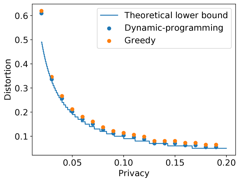
(a) Distribution = Geometric

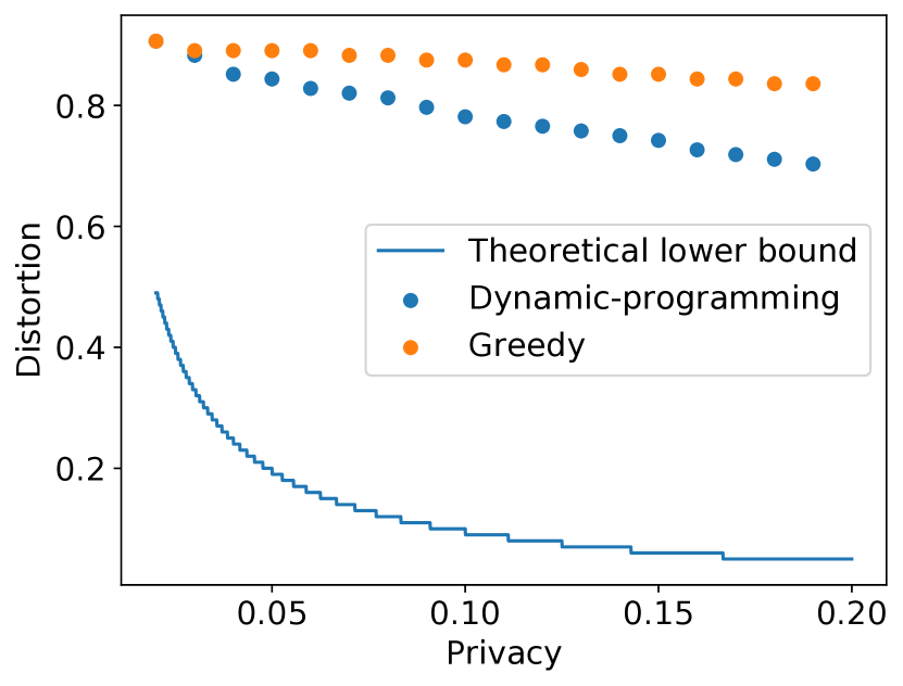
(b) Distribution = Binomial

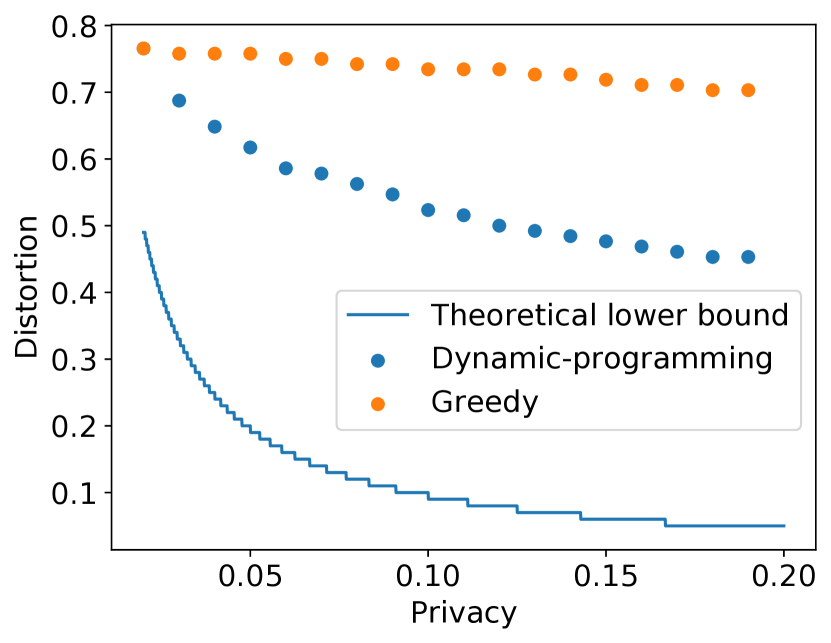
(c) Distribution = Poisson

Figure 15: Privacy-distortion performance of Algorithm 1 and Algorithm 3 for geometric, binomial and Poisson distribution when secret = fraction.

H-B Categorical Distribution

In this section, we consider categorical distributions where the fraction of each bin can be changed freely (as long as they are normalized). We assume that $\theta=\left(p_{1},p_{2},\ldots,p_{C}\right)$ s.t. $p_{i}\in\left[0,1\right]~{}\forall i\in[C]$ and $\sum_{i}p_{i}=1$. Note that this is completely different from the distributions discussed in § H-A where the parameter of the distribution is one-dimensional.

We first analyze the lower bound. Without loss of generality, we assume that we want to protect the fraction of the $j{}$-th bin, i.e. $p_{j}$.

Corollary 8 (Privacy lower bound, secret = fraction of a general discrete distribution).

Consider the secret function $g\left(\theta\right)=p_{1}$. For any $T\in\left(0,1\right)$, when $\Pi_{\epsilon,\omega_{\Theta}}\leq T$, we have $\Delta>\left(\lceil{\frac{1}{T}}\rceil-1\right)\cdot\epsilon$.

The proof is in § H-D. Next, we present the data release mechanism under the following assumption.

Assumption 7.

The prior distribution of $\left(p_{1},\ldots,p_{C}\right)$ is a uniform distribution over all the probability simplex $\{(p_{1},\ldots,p_{C})|p_{i}\in\left[0,1\right)$$\ \forall i\in[C]\text{ and }\sum_{i}p_{i}=1\}$.

Mechanism 5 (For secret = fraction of a categorical distribution).

The parameters of the mechanism are as follows.

$$\mathcal{S}_{p_{1},...,p_{C}} =\bigg{\{}\bigg{(}p_{1}-\frac{t}{C-1},\ldots,p_{j-1}-\frac{t}{C-1},p_{j}+t,$$

$$p_{j+1}-\frac{t}{C-1},\ldots,p_{C}-\frac{t}{C-1}\bigg{)}\bigg{|}t\in\left[-\frac{s}{2},\frac{s}{2}\right)\bigg{\}}~{}~{},$$

$$\theta^{*}_{p_{1},\ldots,p_{C}} =\bigg{(}p_{1}-T,\ldots,p_{j-1}-T,p_{j}+\left(C-1\right)T,$$

$$~{}~{}p_{j+1}-T,\ldots,p_{C+1}-T\bigg{)}~{}~{},$$

where $T=\min\left\{p_{1},\ldots,p_{j-1},p_{j+1},\ldots,p_{C},0\right\}$, and

$$\mathcal{I} =\bigg{\{}\left(p_{1},\ldots,p_{C}\right)\bigg{|}\forall i~{}p_{i}\in\left(-\frac{s}{2\left(C-1\right)},1\right],\sum_{i}p_{i}=1,$$

$$p_{j{}}=\left(k+0.5\right)s,\text{where }k\in\left\{0,1,\ldots,C-1\right\}\bigg{\}}.$$

Here $s>0$ is a hyper-parameter of the mechanism that divides 1.

This data release mechanism achieves the following privacy-distortion trade-off.

Proposition 9.

Under Assumption 7, Mechanism 5 has the following $\Pi_{\epsilon,\omega_{\Theta}}{}$ and $\Delta$ value/bound.

$$\Pi_{\epsilon,\omega_{\Theta}} <\frac{2\epsilon}{s}+1-\left(1-\frac{s}{C-1}\right)^{C-1},$$

$$\Delta =\frac{s}{2}<\left(2+\frac{s}{\epsilon}\right)\Delta_{\text{opt}}.$$

Under the regime $\sup\left(s\right)\rightarrow\mathcal{A}\epsilon$, where $\mathcal{A}$ is a constant larger than $2$, $\Delta$ satisfies

$$\lim_{\sup\left(s\right)\rightarrow\mathcal{A}\epsilon}\Delta<(2+\mathcal{A})\Delta_{\text{opt}}.$$

$\Delta_{\text{opt}}$ is the minimal distortion an optimal data release mechanism can achieve given the privacy Mechanism 5 achieves.

The proof is in § H-E. To ensure that $\Pi_{\epsilon,\omega_{\Theta}}{}<1$, $s$ should satisfy $s>2\epsilon$. According to LABEL:{thm:upperbound_discrete_general_fraction}, the mechanism is order-optimal with multiplicative factor $2+\mathcal{A}$ when $\sup\left(s\right)\rightarrow\mathcal{A}\epsilon$, where $\mathcal{A}>2$.

H-C Proof of Corollary 7

H-C1 Geometric Distribution

Proof.

Let $X_{\theta_{1}}$ and $X_{\theta_{2}}$ be two Geometric random variables with parameters $\theta_{1}$ and $\theta_{2}$ respectively. We assume that $\theta_{1}>\theta_{2}$ without loss of generality. Let $k^{\prime}$ satisfy $\left(1-\theta_{1}\right)^{k^{\prime}}\theta_{1}=\left(1-\theta_{2}\right)^{k^{\prime}}\theta_{2}$ and $k_{0}=\lfloor{k^{\prime}}\rfloor+1$. Then we can get that

$$D\left(X_{\theta_{1}},X_{\theta_{2}}\right) =\frac{1}{2}d_{\text{TV}}\left(\omega_{X_{\theta_{1}}}\|\omega_{X_{\theta_{2}}}\right)$$

$$=\frac{1}{2}\left(1-\theta_{2}\right)^{k_{0}}-\frac{1}{2}\left(1-\theta_{1}\right)^{k_{0}},$$

$$R\left(X_{\theta_{1}},X_{\theta_{2}}\right) =\left|\left(1-\theta_{2}\right)^{j{}}\theta_{2}-\left(1-\theta_{1}\right)^{j{}}\theta_{1}\right|.$$

Therefore, we can get that

$$\ratio=\inf_{\underline{\theta}<\theta_{1}<\theta_{2}\leq\overline{\theta}}\frac{\left(1-\theta_{2}\right)^{k_{0}}-\left(1-\theta_{1}\right)^{k_{0}}}{2\left|\left(1-\theta_{2}\right)^{j{}}\theta_{2}-\left(1-\theta_{1}\right)^{j{}}\theta_{1}\right|}~{}~{}.$$

∎

H-C2 Binomial Distribution

Proof.

Let $X_{\theta_{1}}$ and $X_{\theta_{2}}$ be two binomial random variables with parameters $\theta_{1}$ and $\theta_{2}$ respectively with fixed number of trials $n$. We assume that $\theta_{1}>\theta_{2}$ without loss of generality. Let $k^{\prime}$ satisfy $\binom{n}{k^{\prime}}\theta_{1}^{k^{\prime}}\left(1-\theta_{1}\right)^{n-k^{\prime}}=\binom{n}{k^{\prime}}\theta_{2}^{k^{\prime}}\left(1-\theta_{2}\right)^{n-k^{\prime}}$ and $k_{0}=\lfloor k^{\prime}\rfloor$. We can get that

$$D\left(X_{\theta_{1}},X_{\theta_{2}}\right) =\frac{1}{2}d_{\text{TV}}\left(\omega_{X_{\theta_{1}}}\|\omega_{X_{\theta_{2}}}\right)$$

$$=\frac{1}{2}I_{1-\theta_{2}}\left(n-k_{0},1+k_{0}\right)-\frac{1}{2}I_{1-\theta_{1}}\left(n-k_{0},1+k_{0}\right),$$

$$R\left(X_{\theta_{1}},X_{\theta_{2}}\right) =n\left(\theta_{1}-\theta_{2}\right),$$

where $I$ represents the regularized incomplete beta function.

Therefore, we can get that

$$\ratio=\inf_{\underline{\theta}<\theta_{1}<\theta_{2}\leq\overline{\theta}}\frac{I_{1-\theta_{2}}\left(n-k_{0},1+k_{0}\right)-I_{1-\theta_{1}}\left(n-k_{0},1+k_{0}\right)}{2\left|\binom{n}{j{}}\theta_{2}^{j{}}\left(1-\theta_{2}\right)^{n-j{}}-\binom{n}{j{}}\theta_{1}^{j{}}\left(1-\theta_{1}\right)^{n-j{}}\right|}.$$

∎

H-C3 Poisson Distribution

Proof.

Let $X_{\theta_{1}}$ and $X_{\theta_{2}}$ be two Poisson random variables with parameters $\theta_{1}$ and $\theta_{2}$ respectively. We assume that $\theta_{1}>\theta_{2}$ without loss of generality. Let $k^{\prime}$ satisfy $\theta_{1}^{k^{\prime}}e^{-\theta_{1}}=\theta_{2}^{k^{\prime}}e^{-\theta_{2}}$ and $k_{0}=\lfloor k^{\prime}\rfloor+1$. Then we can get that

$$D\left(X_{\theta_{1}},X_{\theta_{2}}\right) =\frac{1}{2}d_{\text{TV}}\left(\omega_{X_{\theta_{1}}}\|\omega_{X_{\theta_{2}}}\right)$$

$$=\frac{1}{2}Q\left(k_{0},\theta_{2}\right)-\frac{1}{2}Q\left(k_{0},\theta_{1}\right),$$

$$R\left(X_{\theta_{1}},X_{\theta_{2}}\right) =\left|\frac{\theta_{1}^{j}{}e^{-\theta_{1}}}{j{}!}-\frac{\theta_{2}^{j}{}e^{-\theta_{2}}}{j{}!}\right|,$$

where $Q$ is the regularized gamma function.

Therefore, we can get that

$$\ratio=\inf_{\underline{\theta}<\theta_{1}<\theta_{2}\leq\overline{\theta}}\frac{Q\left(k_{0},\theta_{2}\right)-Q\left(k_{0},\theta_{1}\right)}{2\left|\frac{\theta_{1}^{j}{}e^{-\theta_{1}}}{j{}!}-\frac{\theta_{2}^{j}{}e^{-\theta_{2}}}{j{}!}\right|}.$$

∎

H-D Proof of Corollary 8

Proof.

Let $X_{p_{1}^{1},p_{2}^{1},\ldots,p_{C}^{1}}$ and $X_{p_{1}^{2},p_{2}^{2},\ldots,p_{C}^{2}}$ be two categorical random variables. We have

$$\quad D\left(X_{p_{1}^{1},p_{2}^{1},\ldots,p_{C}^{1}},X_{p_{1}^{2},p_{2}^{2},\ldots,p_{C}^{2}}\right)$$

$$=\frac{1}{2}d_{\text{TV}}\left(\omega_{X_{p_{1}^{1},p_{2}^{1},\ldots,p_{C}^{1}}}\|\omega_{X_{p_{1}^{2},p_{2}^{2},\ldots,p_{C}^{2}}}\right)$$

$$\geq\frac{1}{2}\left|p_{j{}}^{1}-p_{j{}}^{2}\right|,$$ (25)

$$\quad R\left(X_{p_{1}^{1},p_{2}^{1},\ldots,p_{C}^{1}},X_{p_{1}^{2},p_{2}^{2},\ldots,p_{C}^{2}}\right)$$

$$=\left|p_{j{}}^{1}-p_{j{}}^{2}\right|.$$

Therefore, we can get that

$$\ratio\geq\frac{1}{2}.$$

∎

H-E Proof of Proposition 9

Proof.

We first focus on the proof for $\Pi_{\epsilon,\omega_{\Theta}}$.

We separate the space of possible data parameters into two regions: $S_{1}=\Big{\{}(p_{1},\ldots,p_{C})|p_{i}\in\left[\frac{s}{2\left(C-1\right)},1-\frac{s}{2\left(C-1\right)}\right]$ $\forall i\in[C]\text{ and }\sum_{i}p_{i}=1\Big{\}}$ and $S_{2}=\left\{(p_{1},\ldots,p_{C})|p_{i}\in\left[0,1\right)~{}\forall i\in[C]\text{ and }\sum_{i}p_{i}=1\right\}\setminus S_{1}$. The high-level idea of our proof is as follows. Note that for any parameter $\theta\in S_{1}$, there exists a $\mathcal{S}_{p_{1},\ldots,p_{C}}$ s.t. $\theta\in\mathcal{S}_{p_{1},\ldots,p_{C}}$ and $\mathcal{S}_{p_{1},\ldots,p_{C}}\subset S_{1}$. Therefore, we can bound the attack success rate if $\theta\in S_{1}$. At the same time, the probability of $\theta\in S_{2}$ is bounded. Therefore, we can bound the overall attacker’s success rate (i.e., $\Pi_{\epsilon,\omega_{\Theta}}$). More specifically, let the optimal attacker be $\hat{g}^{*}$. We have

$$\Pi_{\epsilon,\omega_{\Theta}}{} =\mathbb{P}\left(\hat{g}^{*}\left(\theta^{\prime}\right)\in\left[g\left(\theta\right)-\epsilon,g\left(\theta\right)+\epsilon\right]\right)$$

$$=\int_{\theta\in S_{1}}p(\theta)\mathbb{P}\left(\hat{g}^{*}\left(\theta^{\prime}\right)\in\left[g\left(\theta\right)-\epsilon,g\left(\theta\right)+\epsilon\right]\right)d\theta$$

$$\quad+\int_{\theta\in S_{2}}p(\theta)\mathbb{P}\left(\hat{g}^{*}\left(\theta^{\prime}\right)\in\left[g\left(\theta\right)-\epsilon,g\left(\theta\right)+\epsilon\right]\right)d\theta$$

$$<\frac{2\epsilon}{s}+\left(1-\left(1-\frac{s}{C-1}\right)^{C-1}\right).$$

For the distortion, it is straightforward to get that $\Delta=\frac{s}{2}$ from Eq. 25, and $\Delta_{\text{opt}}>\left(\lceil{\frac{1}{\Pi_{\epsilon,\omega_{\Theta}}{}}}\rceil-1\right)\cdot\epsilon\geq\epsilon$ from Corollary 2. We can get that $\left(\Pi_{\epsilon,\omega_{\Theta}}-\left(1-\left(1-\frac{s}{C-1}\right)^{C-1}\right)\right)\cdot\Delta=\epsilon$ and

$$\Delta =\Delta_{\text{opt}}+\Delta-\Delta_{\text{opt}}$$

$$<\Delta_{\text{opt}}+\Delta-\left(\lceil{\frac{1}{\Pi_{\epsilon,\omega_{\Theta}}}}\rceil-1\right)\cdot\epsilon$$

$$\leq\Delta_{\text{opt}}+\epsilon+\Delta-{{\frac{\epsilon}{\Pi_{\epsilon,\omega_{\Theta}}}}}$$

$$=\Delta_{\text{opt}}+\epsilon+\frac{\left(1-\left(1-\frac{s}{C-1}\right)^{C-1}\right)}{\frac{2\epsilon}{s}+\left(1-\left(1-\frac{s}{C-1}\right)^{C-1}\right)}\cdot\Delta$$

$$=\left(1+\frac{s}{2\epsilon}\left(1-\left(1-\frac{s}{C-1}\right)^{C-1}\right)\right)\left(\Delta_{\text{opt}}+2\ratio\epsilon\right)$$

$$\leq\left(2+\frac{s}{\epsilon}\left(1-\left(1-\frac{s}{C-1}\right)^{C-1}\right)\right)\Delta_{\text{opt}}$$

$$<\left(2+\frac{s}{\epsilon}\right)\Delta_{\text{opt}}.$$

∎

Appendix I Additional Results

In this section, we provide additional results on how released data from our mechanisms can support downstream applications.

We consider the salaries from people with Master’s and PhD degrees in this Kaggle dataset https://www.kaggle.com/datasets/rkiattisak/salaly-prediction-for-beginer. We plot its histogram in Fig. 16. We can see that there are two peaks. They correspond to people with age<=40 and age>40 (see Fig. 17).

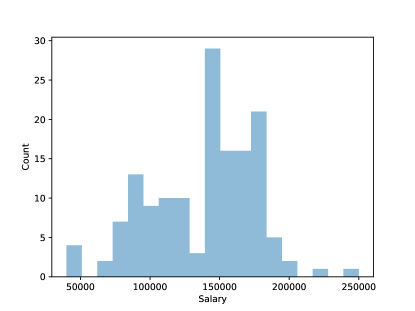
Figure 16: Histogram of salary dataset.

Figure 17: Histogram of salary dataset for people with age <= 40 and > 40.

Figure 18: Histogram of salary dataset for applying the mechanism in § VI-C.

Assume the goal is to release this dataset and preserve the salary difference between people with age<=40 and age>40, while protecting the mean salaries. We can apply our mechanism for mean (§ VI-C) on this dataset. The histogram of the released data is shown in Fig. 18. Data receivers can obtain the salary difference between people with age<=40 and age>40 accurately by computing the difference between the two peaks, while the mean salaries are protected under our mechanism.

Here we use the salary difference between people with age<=40 and age>40 as an example. In general, any downstream tasks that depend only on the “shape” of the distribution will not be affected by our mechanism, since our mechanism shifts all samples by the same amount.

References

• [1] H. L. Lee and S. Whang, “Information sharing in a supply chain,” International journal of manufacturing technology and management, vol. 1, no. 1, pp. 79–93, 2000.
• [2] N. Choucri, S. Madnick, and P. Koepke, “Institutions for cyber security: International responses and data sharing initiatives,” Cambridge, MA: Massachusetts Institute of Technology, 2016.
• [3] J. B. Jacobs and D. Blitsa, “Sharing criminal records: The united states, the european union and interpol compared,” Loy. LA Int’l & Comp. L. Rev., vol. 30, p. 125, 2008.
• [4] J. Deng, W. Dong, R. Socher, L.-J. Li, K. Li, and L. Fei-Fei, “Imagenet: A large-scale hierarchical image database,” in 2009 IEEE conference on computer vision and pattern recognition.   Ieee, 2009, pp. 248–255.
• [5] C. Reiss, J. Wilkes, and J. L. Hellerstein, “Google cluster-usage traces: format+ schema,” Google Inc., White Paper, pp. 1–14, 2011.
• [6] S. Luo, H. Xu, C. Lu, K. Ye, G. Xu, L. Zhang, Y. Ding, J. He, and C. Xu, “Characterizing microservice dependency and performance: Alibaba trace analysis,” in Proceedings of the ACM Symposium on Cloud Computing, 2021, pp. 412–426.
• [7] A. Suri and D. Evans, “Formalizing and estimating distribution inference risks,” arXiv preprint arXiv:2109.06024, 2021.
• [8] A. Suri, Y. Lu, Y. Chen, and D. Evans, “Dissecting distribution inference,” in First IEEE Conference on Secure and Trustworthy Machine Learning, 2023.
• [9] G. Ateniese, L. V. Mancini, A. Spognardi, A. Villani, D. Vitali, and G. Felici, “Hacking smart machines with smarter ones: How to extract meaningful data from machine learning classifiers,” International Journal of Security and Networks, vol. 10, no. 3, pp. 137–150, 2015.
• [10] K. Ganju, Q. Wang, W. Yang, C. A. Gunter, and N. Borisov, “Property inference attacks on fully connected neural networks using permutation invariant representations,” in Proceedings of the 2018 ACM SIGSAC conference on computer and communications security, 2018, pp. 619–633.
• [11] W. Zhang, S. Tople, and O. Ohrimenko, “Leakage of dataset properties in multi-party machine learning.” in USENIX Security Symposium, 2021, pp. 2687–2704.
• [12] S. Mahloujifar, E. Ghosh, and M. Chase, “Property inference from poisoning,” in 2022 IEEE Symposium on Security and Privacy (SP).   IEEE, 2022, pp. 1120–1137.
• [13] H. Chaudhari, J. Abascal, A. Oprea, M. Jagielski, F. Tramèr, and J. Ullman, “Snap: Efficient extraction of private properties with poisoning,” in 2023 IEEE Symposium on Security and Privacy (SP).   IEEE Computer Society, 2022, pp. 1935–1952.
• [14] B. Imana, A. Korolova, and J. Heidemann, “Institutional privacy risks in sharing dns data,” in Proceedings of the Applied Networking Research Workshop, 2021, pp. 69–75.
• [15] Z. Lin, A. Jain, C. Wang, G. Fanti, and V. Sekar, “Using gans for sharing networked time series data: Challenges, initial promise, and open questions,” in Proceedings of the ACM Internet Measurement Conference, 2020, pp. 464–483.
• [16] C. Dwork, F. McSherry, K. Nissim, and A. Smith, “Calibrating noise to sensitivity in private data analysis,” in Theory of Cryptography: Third Theory of Cryptography Conference, TCC 2006, New York, NY, USA, March 4-7, 2006. Proceedings 3.   Springer, 2006, pp. 265–284.
• [17] C. Reiss, J. Wilkes, and J. L. Hellerstein, “Obfuscatory obscanturism: making workload traces of commercially-sensitive systems safe to release,” in 2012 IEEE Network Operations and Management Symposium.   IEEE, 2012, pp. 1279–1286.
• [18] W. Zhang, O. Ohrimenko, and R. Cummings, “Attribute privacy: Framework and mechanisms,” in 2022 ACM Conference on Fairness, Accountability, and Transparency, 2022, pp. 757–766.
• [19] A. Makhdoumi, S. Salamatian, N. Fawaz, and M. Médard, “From the information bottleneck to the privacy funnel,” in 2014 IEEE Information Theory Workshop (ITW 2014).   IEEE, 2014, pp. 501–505.
• [20] I. Issa, A. B. Wagner, and S. Kamath, “An operational approach to information leakage,” IEEE Transactions on Information Theory, vol. 66, no. 3, pp. 1625–1657, 2019.
• [21] H. Wang, L. Vo, F. P. Calmon, M. Médard, K. R. Duffy, and M. Varia, “Privacy with estimation guarantees,” IEEE Transactions on Information Theory, vol. 65, no. 12, pp. 8025–8042, 2019.
• [22] S. Asoodeh, M. Diaz, F. Alajaji, and T. Linder, “Privacy-aware guessing efficiency,” in 2017 ieee international symposium on information theory (isit).   IEEE, 2017, pp. 754–758.
• [23] L. Wasserman and S. Zhou, “A statistical framework for differential privacy,” Journal of the American Statistical Association, vol. 105, no. 489, pp. 375–389, 2010.
• [24] K. Chatzikokolakis, M. E. Andrés, N. E. Bordenabe, and C. Palamidessi, “Broadening the scope of differential privacy using metrics,” in Privacy Enhancing Technologies: 13th International Symposium, PETS 2013, Bloomington, IN, USA, July 10-12, 2013. Proceedings 13.   Springer, 2013, pp. 82–102.
• [25] D. Kifer and A. Machanavajjhala, “Pufferfish: A framework for mathematical privacy definitions,” ACM Transactions on Database Systems (TODS), vol. 39, no. 1, pp. 1–36, 2014.
• [26] Y. Kawamoto and T. Murakami, “Local obfuscation mechanisms for hiding probability distributions,” in Computer Security–ESORICS 2019: 24th European Symposium on Research in Computer Security, Luxembourg, September 23–27, 2019, Proceedings, Part I 24.   Springer, 2019, pp. 128–148.
• [27] M. Chen and O. Ohrimenko, “Protecting global properties of datasets with distribution privacy mechanisms,” arXiv preprint arXiv:2207.08367, 2022.
• [28] H. Yamamoto, “A source coding problem for sources with additional outputs to keep secret from the receiver or wiretappers (corresp.),” IEEE Transactions on Information Theory, vol. 29, no. 6, pp. 918–923, 1983.
• [29] G. Smith, “On the foundations of quantitative information flow,” in International Conference on Foundations of Software Science and Computational Structures.   Springer, 2009, pp. 288–302.
• [30] M. S. Alvim, K. Chatzikokolakis, A. McIver, C. Morgan, C. Palamidessi, and G. Smith, “Additive and multiplicative notions of leakage, and their capacities,” in 2014 IEEE 27th Computer Security Foundations Symposium.   IEEE, 2014, pp. 308–322.
• [31] F. P. Calmon, A. Makhdoumi, and M. Médard, “Fundamental limits of perfect privacy,” in 2015 IEEE International Symposium on Information Theory (ISIT).   IEEE, 2015, pp. 1796–1800.
• [32] S. Asoodeh, M. Diaz, F. Alajaji, and T. Linder, “Information extraction under privacy constraints,” Information, vol. 7, no. 1, p. 15, 2016.
• [33] J. Liao, O. Kosut, L. Sankar, and F. du Pin Calmon, “Tunable measures for information leakage and applications to privacy-utility tradeoffs,” IEEE Transactions on Information Theory, vol. 65, no. 12, pp. 8043–8066, 2019.
• [34] S. Saeidian, G. Cervia, T. J. Oechtering, and M. Skoglund, “Pointwise maximal leakage,” in 2022 IEEE International Symposium on Information Theory (ISIT).   IEEE, 2022, pp. 626–631.
• [35] G. R. Kurri, L. Sankar, and O. Kosut, “An operational approach to information leakage via generalized gain functions,” arXiv preprint arXiv:2209.13862, 2022.
• [36] A. Gilani, G. R. Kurri, O. Kosut, and L. Sankar, “$(\alpha,\beta)$-leakage: A unified privacy leakage measure,” arXiv preprint arXiv:2304.07456, 2023.
• [37] B. Rassouli and D. Gündüz, “On perfect privacy,” IEEE Journal on Selected Areas in Information Theory, vol. 2, no. 1, pp. 177–191, 2021.
• [38] A. Zamani, T. J. Oechtering, and M. Skoglund, “Bounds for privacy-utility trade-off with non-zero leakage,” in 2022 IEEE International Symposium on Information Theory (ISIT).   IEEE, 2022, pp. 620–625.
• [39] B. Rassouli and D. Gündüz, “Optimal utility-privacy trade-off with total variation distance as a privacy measure,” IEEE Transactions on Information Forensics and Security, vol. 15, pp. 594–603, 2019.
• [40] S. A. Mario, K. Chatzikokolakis, C. Palamidessi, and G. Smith, “Measuring information leakage using generalized gain functions,” in 2012 IEEE 25th Computer Security Foundations Symposium.   IEEE, 2012, pp. 265–279.
• [41] S. Asoodeh, M. Diaz, F. Alajaji, and T. Linder, “Estimation efficiency under privacy constraints,” IEEE Transactions on Information Theory, vol. 65, no. 3, pp. 1512–1534, 2018.
• [42] M. Arjovsky, S. Chintala, and L. Bottou, “Wasserstein generative adversarial networks,” in International conference on machine learning.   PMLR, 2017, pp. 214–223.
• [43] Z. Lin, A. Khetan, G. Fanti, and S. Oh, “Pacgan: The power of two samples in generative adversarial networks,” Advances in neural information processing systems, vol. 31, 2018.
• [44] R. Bellman, “Dynamic programming,” Science, vol. 153, no. 3731, pp. 34–37, 1966.
• [45] C. Esteban, S. L. Hyland, and G. Rätsch, “Real-valued (medical) time series generation with recurrent conditional gans,” arXiv preprint arXiv:1706.02633, 2017.
• [46] Y. Yin, Z. Lin, M. Jin, G. Fanti, and V. Sekar, “Practical gan-based synthetic ip header trace generation using netshare,” in Proceedings of the ACM SIGCOMM 2022 Conference, 2022, pp. 458–472.
• [47] J. Jordon, J. Yoon, and M. Van Der Schaar, “Pate-gan: Generating synthetic data with differential privacy guarantees,” in International conference on learning representations, 2018.
• [48] J. Yoon, D. Jarrett, and M. Van der Schaar, “Time-series generative adversarial networks,” Advances in neural information processing systems, vol. 32, 2019.
• [49] Google, “Web traffic time series forecasting,” 2018, https://www.kaggle.com/c/web-traffic-time-series-forecasting.
• [50] F. C. Commission, “Raw data - measuring broadband america - seventh report,” 2018, https://www.fcc.gov/reports-research/reports/measuring-broadband-america/raw-data-measuring-broadband-america-seventh.
• [51] A. Ghosh and R. Kleinberg, “Inferential privacy guarantees for differentially private mechanisms,” arXiv preprint arXiv:1603.01508, 2016.