Abstract

Prediction models can perform poorly when deployed to target distributions different from the training distribution. To understand these operational failure modes, we develop a method, called DIstribution Shift DEcomposition (DISDE), to attribute a drop in performance to different types of distribution shifts. Our approach decomposes the performance drop into terms for 1) an increase in harder but frequently seen examples from training, 2) changes in the relationship between features and outcomes, and 3) poor performance on examples infrequent or unseen during training. Empirically, we demonstrate how our method can 1) inform potential modeling improvements across distribution shifts for employment prediction on tabular census data, and and 2) help to explain why certain domain adaptation methods fail to improve model performance for satellite image classification.

1 Introduction

Prediction models operate on data distributions different from those seen during training, but often perform worse on these target distributions than on the original training distribution. For example, Wong et al. [101] observed EPIC’s sepsis risk assessment model, which is deployed across hundreds of hospitals in the US, performs “substantially worse” in the wild compared to vendor claims. The lack of reliability in predictive performance across distributions has been documented in many domains including healthcare [55, 4, 107, 16, 101], loan approval [38], wildlife conservation [6], and education [1]. Similar performance degradation has been widely observed in computer vision and natural language processing (NLP) settings [75, 60, 93, 86, 61, 54]. As decisions are increasingly made based on model predictions, we need rigorous and scalable tools for diagnosing model failures in order to guide resources toward effective model improvements.

Different distribution shifts require different solutions. Understanding why model performance worsened is a fundamental step for informing subsequent methodological and operational interventions. While there are multiple taxonomies for discussing distribution shifts [58, 84, 97], we focus on a popular one: we categorize distribution shifts as either a change in the marginal distribution of the covariates ($X$), or a change in the conditional relationship between the label and covariate ($Y\mid X$). Since real distribution shifts occur as a combination of both types, we develop a framework for understanding how much performance degradation is assigned to each type in order to best improve model performance.

There are many reasons why the marginal distribution of the covariates $X$ can change. For example, training and target data may be collected from different points in time and space, marginalized groups may be underrepresented in the training data, or population demographics may change over time [87, 7, 17, 14]. If the shift in the distribution of covariates $X$ is small, then domain adaptation [87], warm-starting/fine-tuning [21, 102], or importance sampling-based reweighting [3, 68, 27] approaches can be effective. If there is a more extreme form of covariate shift, such as the presence of target covariate values $X$ that were unseen during training, then it may be necessary to collect data and labels over this new group.

On the other hand, shifts in the relationship between the outcomes and covariates $Y\mid X$ can be caused by changes in measurement errors, changes in user behavior, and unrecorded confounding factors whose distributions change [38]. In these cases, recent works on explicit causal or worst-case modeling may be helpful [103, 35, 12, 79, 9, 51, 100, 28]. When methods like these cannot address the performance drop, existing data from the training distribution may not be useful for the target distribution, so that further data collection and labeling may be necessary. Alternatively, the covariates $X$ may not be predictive of the outcome between both distributions, requiring changes in feature engineering.

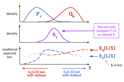
Figure 1: Diagnosing distribution shifts: Illustration of a key idea on a one-dimensional covariate $X$: we can only compare $Y\mid X$ for training vs test, and predictive performances thereof, on $X$’s that are common between both distributions. We use $L$ to denote the loss.

Towards diagnosing model performance degradations, we propose a new framework which we call DIstribution Shift DEcomposition (DISDE). At a high level, performance degradation attributed to $Y\mid X$ shift is obtained by varying $Y\mid X$ between training and test while keeping the distribution of $X$ fixed, and performance degradation attributed to $X$ shift is obtained by varying the distribution of $X$ while keeping $Y\mid X$ fixed. In order to make these comparisons, observe that the training and target distributions of $Y\mid X$—and predictive performances thereof—can only be compared over values of $X$ that are sufficiently common between training and target (see Figure 1). Thus, one core aspect of our framework is the notion of a shared distribution between $X$’s of the training and target distributions over which it is easy to estimate model performace (Section 3). Using this shared distribution, we decompose the performance degradation into three terms: one for changes in the relationship between $X$ and $Y$ on this shared distribution, and two for changes in the distribution of $X$ from both the training and target distributions to the shared distribution.

By attributing loss to different distribution shifts, our approach goes beyond detecting changes in the distribution, as DISDE quantifies how much each type of shift affects performance. The first term in our decomposition (Equation (2.1) to come) measures performance degradation due to an increase in the frequency of harder values of $X$ that are common between training and target distributions (an $X$ shift). The second term measures performance degradation due to changes in the relationship between $X$ and $Y$ (a $Y\mid X$ shift), over values of $X$ common to both distributions. The third measures performance degradation due to poor performance on values of $X$ that are infrequent or unseen during training (an $X$ shift).

One important aspect of DISDE is precisely defining and estimating the shared distribution. As we discuss in Section 2.2, we define this shared distribution so that it has the largest mass on values of $X$ that are most likely in both training and target. Our approach is motivated by weighting schemes in causal inference that focus on a subset of the population where treatment and control units are similar enough to compare [23, 57]. To estimate this shared distribution, we train a binary classifier to predict between the training and target distributions using features $X$, which we refer to as the auxiliary domain classifier. Using this classifier, we can reweight samples from training and test into the shared distribution; we operationalize “common” examples across train and target as those that cannot be confidently and correctly classified as being from either training or target.

Our approach is general, and DISDE can be extended to attribute performance degradation to use $Z$ in place of $X$ for any flexible feature vector $Z$ (Section 2.3). For example, $Z$ can be a subset of covariates (Section 4.1.1, a (learned) feature mapping (Section 4.2), some other piece of metadata, or even the label $Y$ itself, turning DISDE into a method for diagnosing label shift.

We apply our method to three real distribution shifts in Section 4. In the first example (Section 4.1), we predict employment from tabular census data [26] and study how predictive performance deteriorates over a variety of natural and semi-synthetic distribution shifts. We illustrate how DISDE gives correct performance attributions, and how it can inform different ways of improving performance on the target distribution. In the second example (Section 4.2), we study satellite image classification for land or building use (FMoW-WILDS [50]). We use DISDE to diagnose why a popular domain adaptation method, DANN [34], does not do better than standard empirical risk minimization over spatiotemporal shifts, even though DANN is designed to perform well over distribution shifts. This example also demonstrates how DISDE can be scaled to high-dimensional, complex data such as images. Overall, our experiments show how DISDE can be used to guide modeling improvements and to provide insight where specific interventions fail, and also to understand learned feature representations.

Finally, we analyze the large-sample statistical properties of the proposed estimation method in Section 5. By leveraging results from the semiparametric statistics literature [66], we give a central limit theorem for our estimator even when the auxiliary domain classifier is estimated nonparametrically. This provides a principled approach for generating confidence intervals in DISDE. We compare the asymptotic variance of our estimator to lower bounds under a well-developed calculus for statistical functionals [10, 64, 48] to confirm that our proposed approach is statistically efficient, under suitable regularity assumptions on the auxiliary classifier.

To summarize, our main contributions are as follows:

• We introduce a simple method, DIstribution Shift DEcomposition (DISDE), to attribute a change in model performance across a distribution shift to $X$ and $Y\mid X$ shifts.

• We empirically demonstrate how DISDE can inform model improvements across distribution shifts on both tabular and image data.

• We analyze the asymptotic properties of DISDE, provide a principled way to estimate confidence intervals, and show efficiency of our estimator under certain conditions.

As there is a large body of work on distribution shifts across multiple fields, we defer a discussion of related literature to Section 6 where we situate the current work in a broader context.

2 Decomposing the performance degradation

Consider a model $f$ that predicts outcome $Y$ from covariates $X$. Let $f$ be trained on data $(X,Y)$ drawn from the training distribution $P$. Let $\ell(f(x),y)$ be a loss function denoting a notion of predictive error (e.g. 0-1 error, cross-entropy loss). We consider a situation in which we observe a performance degradation from $P$ to a target distribution $Q$, i.e. $\mathbb{E}_{Q}[\ell(f(X),Y)]>\mathbb{E}_{P}[\ell(f(X),Y)]$. As a motivating example, consider a model trained to predict employment status based on demographic information, which could be important for economic policy-making and marketing.

Training accuracy	70%
Target accuracy	61%

Table 1: Performance degradation in the employment prediction example

Due to operational constraints, the model may be trained using data collected from one state, such as West Virginia (training distribution), but used across a range of different states, including Maryland (target distribution). In such cases, we may only have enough labeled data from Maryland to evaluate a model, but not enough to train a new model. As we show in Table 1 and further investigate in Section 4.1, the model trained on West Virginia performs poorly on Maryland. As collecting more training data from Maryland is costly, we seek to understand the performance drop to determine how best to improve our models for use on Maryland.

To understand how the distribution shift led to such a performance degradation, we attribute the performance degradation to shifts in the marginal distribution of $X$ and to the conditional distribution of $Y\mid X$. The natural objects to quantify $X$ and $Y\mid X$ shifts are, respectively, the marginal distributions of $X$, $P_{X}(\cdot)$ and $Q_{X}(\cdot)$, and the conditional risks on $P$ and $Q$,

$$R_{\mu}(x)\mathrel{\mathop{\mathchar 58\relax}}=\mathbb{E}_{\mu}[\ell(f(X),Y)\mid X=x]~{}\mbox{for}~{}\mu=P,Q.$$

However, there are two practical issues with studying these quantities directly. First, estimation of these functions is a challenging density estimation or nonparametric regression problem. As in our motivating example above, one of our primary use cases is when we only have limited labeled target data from $Q$. Second, even if we could derive reasonable estimates of these functions, it would be difficult to display them in a way that would be useful for a human to understand, especially for $X$ of larger dimension. Therefore, we need to summarize the infinite dimensional quantities $\{R_{P}(\cdot),R_{Q}(\cdot),P_{X},Q_{X}\}$ in a practical and statistically efficient way.

Our approach is the following: to attribute loss to $X$ shift, compare the conditional risk $R_{P}(x)$ (resp. $R_{Q}(x)$) under different marginal distributions of $X$. Then, to attribute loss to $Y\mid X$ shift, compare $R_{P}(x)$ and $R_{Q}(x)$ under the same marginal distribution of $X$. Recalling Figure 1, the main challenge in doing this is that $R_{P}(x)$ (resp. $R_{Q}(x)$) is only well-defined for values of $x$ that are in the support of $P_{X}$ (resp. $Q_{X}$). Therefore, when comparing performance $R_{Q}(x)-R_{P}(x)$ across different $Y\mid X$ distributions, we need to define a shared distribution $S_{X}$ with support contained in both $P_{X}$ and $Q_{X}$. We temporarily defer a discussion on different choices of formulations for shared distributions to Section 2.2 and first outline our approach for any fixed definition of the shared distribution $S_{X}$.

We thus attribute performance degradation to $Y\mid X$ by comparing the averages of the conditional risks $R_{P}(X)$ and $R_{Q}(X)$ on the marginal distribution $S_{X}$ as

$$\mathbb{E}_{S_{X}}[R_{\bm{P}}(X)]~{}\mbox{versus}~{}\mathbb{E}_{S_{X}}[R_{\bm{Q}}(X)].$$

Then, for $X$ shift, we can construct a well-defined comparison of the average of $R_{P}(X)$ under the two marginal distributions $P_{X}$ and $S_{X}$,

$$\mathbb{E}_{\bm{P_{X}}}[R_{P}(X)]~{}\mbox{versus}~{}\mathbb{E}_{\bm{S_{X}}}[R_{P}(X)],$$

and similarly for the average of $R_{Q}(X)$ under the marginal distributions $Q_{X}$ and $S_{X}$. Altogether, we can decompose the change in expected loss from $P$ to $Q$ as the telescoping sum

$$\mathbb{E}_{Q}[\ell(f(X),Y)]-\mathbb{E}_{P}[\ell(f(X),Y)] =\mathbb{E}_{S_{X}}[R_{P}(X)]-\mathbb{E}_{P}[R_{P}(X)] X P\rightarrow S$$ shift () (2.1a)

$$\hskip 15.00002pt+\mathbb{E}_{S_{X}}[R_{Q}(X)-R_{P}(X)] Y\mid X$$ shift (2.1b)

$$\hskip 15.00002pt+\mathbb{E}_{Q}[R_{Q}(X)]-\mathbb{E}_{S_{X}}[R_{Q}(X)]. X S\rightarrow Q$$ shift () (2.1c)

The telescoping sum is illustrated in Figure 2, where the bolded arrows represent the terms in Equation (2.1).

Figure 2: Diagram of decomposition: left to right represents changing $X$ distribution from $P_{X}$ to $S_{X}$ to $Q_{X}$. Up to down represents changing $Y\mid X$ from $P_{Y|X}$ to $Q_{Y|X}$, by replacing $R_{P}(X)$ with $R_{Q}(X)$. The bolded arrows correspond to the decomposition terms we propose, where each arrow $A\to B$ represents the difference $B-A$.

2.1 Interpreting the decomposition (2.1)

We provide intuition for the terms in Equation (2.1) and discuss ways to improve test performance for when each term is large.

2.1.1 $X$ shift ($P\to S$) term

$\mathbb{E}_{S_{X}}[R_{P}(X)]-\mathbb{E}_{P_{X}}[R_{P}(X)]$ is the expected difference in loss under $P_{Y|X}$ between examples with $X\sim P_{X}$ and $X\sim S_{X}$. This term is large if the model performs worse on covariates $X$ common in both $P_{X}$ and $Q_{X}$ under $P_{Y|X}$, compared to covariates from $P_{X}$. This can happen if e.g. $Q_{X}$ has more of the hard examples from $P_{X}$. If $P_{Y|X}=Q_{Y|X}$, then we expect the shared data $X\sim S_{X}$ to be able to inform good models under $Q_{X}$, e.g. by using domain adaptation methods.

In the context of the employment prediction problem described at the beginning of the section, a large $X$ shift ($P\to S$) term could indicate that the change in loss between West Virginia and Maryland is largely due to Maryland having more people than West Virginia of demographics that were difficult for the model to predict. In this case, we may refit the model by reweighting training observations from West Virginia to resemble the population in Maryland.

2.1.2 $Y\mid X$ shift term

$\mathbb{E}_{S_{X}}[R_{Q}(X)-R_{P}(X)]$ is the expected difference in loss between $Q_{Y|X}$ and $P_{Y|X}$ over the shared covariates $X\sim S_{X}$ common across $P_{X}$ and $Q_{X}$. We expect this term to be large if the loss is larger under $Q_{Y|X}$ than under $P_{Y|X}$ over shared covariates $X\sim S_{X}$. Loosely speaking, this can happen if the relationship $Y\mid X$ changes unfavorably from $P$ to $Q$ for the prediction model $f$. In cases with a large $Y\mid X$ shift term, it may be necessary to collect and label new data over $Q_{Y|X}$, or to modify the set of covariates.

In the context of employment prediction, a large $X$ shift ($S\to Q$) term may indicate that the change in model loss is largely due to a difference in the likelihood of whether a person of the same demographics is employed, in West Virginia vs Maryland, for people whose demographics are common in both states. Solving this may require investing in a new data collection campaign in Maryland large enough to train a new model. Alternatively, we may search for new covariates $X^{\prime}$ such that $Y\mid(X,X^{\prime})$ remains similar across West Virginia (training) and Maryland (target) and train a new model that also uses the additional features $X^{\prime}$.

2.1.3 $X$ shift ($S\to Q$) term

$\mathbb{E}_{Q_{X}}[R_{Q}(X)]-\mathbb{E}_{S_{X}}[R_{Q}(X)]$ is the expected difference in loss under $Q_{Y|X}$ between examples $X\sim S_{X}$ and $X\sim Q_{X}$. Consider values of $X$ that are frequent in the target distribution $Q_{X}$ but infrequent or unseen in the training distribution $P_{X}$. We colloquially refer to these as “newer examples”, which include unseen examples as well as values of $X$ that are relatively more common in $Q_{X}$ compared to $S_{X}$. The $X$ shift ($S\to Q$) term is large if the model performs poorly incurs higher loss on such “newer examples” under $Q_{Y|X}$. This type of performance degradation can be addressed by collecting “newer examples” and retraining or fine-tuning a model on these examples.

In our employment prediction example, a large $X$ shift ($S\to Q$) term could indiciate that the change in model loss is largely due to Maryland having people of demographics that are unseen or uncommon West Virginia, that are also difficult for the model to predict. A potential solution involves conducting a survey of employment status in Maryland targeting demographic groups that were rarely observed in West Virginia.

2.1.4 Comparisons

The two $X$ shift terms both attribute performance degradation to $X$ shift, but differ in the following way: the $X$ shift ($P\to S$) term contains performance degradation from $P_{X}$ having support on examples with low loss where $Q_{X}$ does not, and the $X$ shift ($S\to Q$) term contains performance degradation from $Q_{X}$ having support on examples with high loss where $P_{X}$ does not. However, beyond this distinction, how much a value of $X$ is “allocated” to either of these terms may not necessarily be meaningful. Another difference between the two $X$ shift terms is that the $X$ shift ($P\to S$) term uses $P_{Y|X}$ while the $X$ shift ($S\to Q$) term uses $Q_{Y|X}$. Because of this, one part of the $X$ shift (from $P_{X}$ to $S_{X}$) is measured under $P_{Y|X}$, while the rest (fom $S_{X}$ to $Q_{X}$) is measured under $Q_{Y|X}$. Again, this distinction can be somewhat arbitrary. Despite these subtleties, in practice, it may be helpful to think of these two terms as qualitatively similar when diagnosing a model’s failures in practice.

For concrete examples of decompositions for different $Y\mid X$ vs $X$ shifts and the corresponding modeling interventions, please refer to the experiments in Section 4.1.

2.2 Defining the shared distribution $S_{X}$

To operationalize our approach, we choose a specific shared distribution $S_{X}$ over $X$ whose support is contained in that of $P_{X}$ and $Q_{X}$. An ideal choice of shared distribution is one that has higher density when the $P_{X}$ and $Q_{X}$ both have higher density, and lower density when either of $P_{X}$ or $Q_{X}$ has a low density. This sharpens the above requirement of shared support to a stronger notion of sharing regions of high density. Letting $p_{X}$, $q_{X}$, and $s_{X}$ be the densities of $X$ under $P$, $Q$, and $S$ under a suitable base measure, consider choosing

$$s_{X}(x)\propto\frac{p_{X}(x)q_{X}(x)}{p_{X}(x)+q_{X}(x)}.$$ (2.2)

However, there are many shared distributions that satisfy our criteria, and the above choice is not unique. For example, other choices include

$$s_{X}(x) \propto\min\{p_{X}(x),q_{X}(x)\}~{}~{}~{}\mbox{or}~{}~{}~{}$$ (2.3a)

$$s_{X}(x) \propto\begin{cases}p_{X}(x)+q_{X}(x)~{}~{}&\mbox{if}~{}\min\left\{\frac{p_{X}(x)}{q_{X}(x)},\frac{q_{X}(x)}{p_{X}(x)}\right\}\geq\epsilon\\ 0~{}~{}&\mbox{otherwise}\end{cases}$$ (2.3b)

for some $\epsilon>0$. The shared distribution (2.3b) is particularly intuitive as it defines “shared” examples as those that have sufficiently high likelihood ratios. However, it is difficult to operationalize as it depends on an arbitrary choice of $\epsilon>0$. Observe that for all of the above definitions of $S_{X}$, if $P_{X}=Q_{X}$, then $S_{X}=P_{X}=Q_{X}$. Additionally observe that Equations (2.2) and (2.3a) become similar (up to a scaling factor) for regions of $x$ where $p_{X}(x)\gg q_{X}(x)$ or $p_{X}(x)\ll q_{X}(x)$.

For the shared distributions listed above, our decomposition can be estimated by reweighting data from $P$ and $Q$ to approximate samples from the shared distribution, as described in more detail in Section 3. We use an auxiliary binary classifier between $P$ and $Q$ to learn these importance weights, which are bounded under weak assumptions and provide low (asymptotic) variance estimates for $\mathbb{E}_{S_{X}}[R_{P}(X)]$ and $\mathbb{E}_{S_{X}}[R_{Q}(X)]$. Most of our method extends to the alternative shared distributions (2.3) in place of the one in Equation (2.2), and in practice we find that the qualitative conclusions obtained from our approach are not very sensitive to the specific choice of shared distribution (Appendix F). For ease of exposition, we focus on the shared distribution defined in Equation (2.2).

2.3 Generalization to other decompositions

Our approach generalizes to any choice of mapping $(X,Y)\mapsto Z$ in place of $X$. This generalization attributes performance degradation from $P$ to $Q$ to changes in the marginal distributions of $Z$, and to changes in the conditional distribution of the data $(X,Y)$ given $Z$. Specifically, we can generalize $R_{\mu}(z)$ to be

$$R_{\mu}(z)\mathrel{\mathop{\mathchar 58\relax}}=\mathbb{E}_{\mu}[\ell(f(X),Y)|Z=z]~{}\mbox{for}~{}\mu=P,Q,$$

and re-write the decomposition as

$$\mathbb{E}_{Q}[\ell(f(X),Y)]-\mathbb{E}_{P}[\ell(f(X),Y)] =\mathbb{E}_{S_{Z}}[R_{P}(Z)]-\mathbb{E}_{P}[R_{P}(Z)] Z P\to S$$ shift () (2.4a)

$$\hskip 15.00002pt+\mathbb{E}_{S_{Z}}[R_{Q}(Z)-R_{P}(Z)] (X,Y)\mid Z$$ shift (2.4b)

$$\hskip 15.00002pt+\mathbb{E}_{Q}[R_{Q}(Z)]-\mathbb{E}_{S_{Z}}[R_{Q}(Z)]. Z S\to Q$$ shift () (2.4c)

This generalization allows us to provide a richer diagnostic for machine learning applications. For example, when $Z=\phi(X)$ where $\phi(\cdot)$ is a feature mapping (e.g. from the prediction model $f$), large performance degradation attributed to $Y\mid\phi(X)$ shift may imply the relationship between $Y$ and $\phi(X)$ is not stable between training and target. This could suggest that those features are not appropriate for prediction across both distributions. This is demonstrated in experiments in Section 4.1.1, where $Z$ is a subset of $X$, and Section 4.2, where $Z$ is a learned feature representation.

We can also use metadata as $Z$. In this case, we can think of $X$ as containing both metadata and “regular” data, and $f(\cdot)$ to only use regular data. As an additional example, we can use $Y$ as $Z$, in which case the decomposition measures label shift [58].

The methodological (Section 3) and theoretical (Section 5) results in the rest of the paper extend immediately to using $Z$ instead of $X$; we would replace $\pi(x),R_{P}(x),R_{Q}(x)$ with $\pi(z),R_{P}(z),R_{Q}(z)$ and similarly for their estimates.

3 Estimation

In our decomposition (2.1), each term corresponds to the difference of consecutive pairs of $\mathbb{E}_{P}[R_{P}(X)]$, $\mathbb{E}_{S_{X}}[R_{P}(X)]$, $\mathbb{E}_{S_{X}}[R_{Q}(X)]$, $\mathbb{E}_{Q}[R_{Q}(X)]$, as illustrated in Figure 2. The first and last terms are easily estimated by the empirical average of losses over $(X_{i},Y_{i})\stackrel{{\scriptstyle\rm iid}}{{\sim}}P$ and $(X_{j},Y_{j})\stackrel{{\scriptstyle\rm iid}}{{\sim}}Q$, respectively. Thus, we focus on the estimation of the middle two terms

$$\mathbb{E}_{S_{X}}[R_{P}(X)]~{}~{}~{}\mbox{and}~{}~{}~{}\mathbb{E}_{S_{X}}[R_{Q}(X)].$$ (3.1)

A key statistical challenge is that we do not have access to samples from the shared distribution $S_{X}$ since it is a fictitious quantity defined for interpretating the performance degradation. As we only have samples $X_{i}\stackrel{{\scriptstyle\rm iid}}{{\sim}}P$ and $X_{j}\stackrel{{\scriptstyle\rm iid}}{{\sim}}Q$, our strategy is to reweight them to approximate samples from $S_{X}$, which in turn allows us to estimate the two terms (3.1). To see this, rewrite our estimands as

$$\theta_{P}\mathrel{\mathop{\mathchar 58\relax}}=\mathbb{E}_{S_{X}}[R_{P}(X)] =\mathbb{E}_{P}\left[R_{P}(X)\frac{dS_{X}}{dP_{X}}(X)\right]=\mathbb{E}_{P}\left[\ell(f(X),Y)\frac{dS_{X}}{dP_{X}}(X)\right]$$ (3.2a)

$$\theta_{Q}\mathrel{\mathop{\mathchar 58\relax}}=\mathbb{E}_{S_{X}}[R_{Q}(X)] =\mathbb{E}_{Q}\left[R_{Q}(X)\frac{dS_{X}}{dQ_{X}}(X)\right]=\mathbb{E}_{Q}\left[\ell(f(X),Y)\frac{dS_{X}}{dQ_{X}}(X)\right].$$ (3.2b)

Once we obtain estimates for the importance weights $\frac{dS_{X}}{dP_{X}}$ and $\frac{dS_{X}}{dQ_{X}}$, we estimate $\theta_{P}$ and $\theta_{Q}$ by using an empirical plug-in of Equation (3.2) above, and as described in Algorithm 1.

To calculate the importance weights $\frac{dS_{X}}{dP_{X}},\;\frac{dS_{X}}{dQ_{X}}$, we can use an auxiliary domain classifier. Recalling the definition of the shared distribution $S_{X}$ (2.2), we have

$$\frac{dS_{X}}{dP_{X}}(x)\propto\frac{q(x)}{p(x)+q(x)}~{}~{}~{}\mbox{and}~{}~{}~{}\frac{dS_{X}}{dQ_{X}}(x)\propto\frac{p(x)}{p(x)+q(x)}.$$ (3.3)

Now observe that $\frac{dS_{X}}{dP_{X}}\propto\frac{q(x)}{p(x)+q(x)}$ corresponds to the probability that a data point with value $x$ drawn from an even mixture distribution of $P_{X}$ and $Q_{X}$ actually came from $Q_{X}$, which can be estimated using any machine learning classifier that outputs class probabilities (e.g. neural networks, random forests, logistic regression), as we can consider coming from $Q_{X}$ vs $P_{X}$ to be the classes for classification. We can thus leverage a broad set of scalable and effective machine learning methods to estimate these probabilities.

Observe also that weighting samples from $P_{X}$ by the classifier probability that it came from $Q_{X}$ is consistent with the intuition that data points likely to be from the shared distribution $S_{X}$ are those that are difficult to classify correctly as being from $P_{X}$ or $Q_{X}$.

In practice, we may not have an even mixture of samples from $P_{X}$ and $Q_{X}$ on which to learn the auxiliary domain classifier, e.g. if we have fewer samples from target than training. In such cases, we can use standard techniques from the label-shift literature to adjust the base rate [32]. To help formalize this, define the following:

$$\begin{split}&\alpha^{*}~{}~{}\mbox{is the proportion of the pooled data that comes from}~{}Q_{X}\\ &T=\begin{cases}0~{}~{}&\mbox{if}~{}\tilde{X}~{}\mbox{is from}~{}P_{X}\\ 1~{}~{}&\mbox{if}~{}\tilde{X}~{}\mbox{is from}~{}Q_{X}\end{cases}\\ &\pi^{*}(x)\mathrel{\mathop{\mathchar 58\relax}}=\mathbb{P}(T=1\mid\tilde{X}=x)=\frac{\alpha^{*}q(x)}{\alpha^{*}q(x)+(1-\alpha^{*})p(x)}\end{split}$$ (3.4)

where the last equality is by Bayes’ rule, and $\mathbb{P}(\cdot)$ is probability under the distribution of the observed data. As before, $\pi^{*}(x)$ can also be interpreted as the probability output from the true domain classifier. Then we can express the importance ratios as follows:

$$\frac{dS_{X}}{dP_{X}}(x) \propto\frac{\pi(x)}{(1-\alpha)\pi(x)+\alpha(1-\pi(x))}=\mathrel{\mathop{\mathchar 58\relax}}w_{P}(\pi(x),\alpha)$$ (3.5a)

$$\frac{dS_{X}}{dQ_{X}}(x) \propto\frac{1-\pi(x)}{(1-\alpha)\pi(x)+\alpha(1-\pi(x))}=\mathrel{\mathop{\mathchar 58\relax}}w_{Q}(\pi(x),\alpha).$$ (3.5b)

1 Estimate $\mathbb{E}_{P}[R_{P}(X)]$ and $\mathbb{E}_{Q}[R_{Q}(X)]$ using data $(X_{i},Y_{i})\sim P$, with $i=1,\ldots,n_{P}$, and $(X_{j},Y_{j})\sim Q$, with $j=1,\ldots,n_{Q}$:

$$\mathbb{E}_{P}[R_{P}(X)]\approx\frac{1}{n_{P}}\sum_{i=1}^{n_{P}}\ell(f(X_{i}),Y_{i})~{}~{}\mbox{and}~{}~{}\mathbb{E}_{Q}[R_{Q}(X)]\approx\frac{1}{n_{Q}}\sum_{j=1}^{n_{Q}}\ell(f(X_{j}),Y_{j}).$$

2Estimate $\widehat{\alpha}=n_{Q}/(n_{P}+n_{Q})$.

3Estimate $\widehat{\pi}(x)\approx\mathbb{P}(T=1|X=x)$ by training a classifier on $X$’s from $P_{X}$ vs $Q_{X}$, where samples from $P_{X}$ and $Q_{X}$ are given labels 0 and 1, respectively.

4Calculate importance weights proportional to $\frac{dS_{X}}{dP_{X}}$ and $\frac{dS_{X}}{dQ_{X}}$:

$$w_{P}(\widehat{\pi}(x),\widehat{\alpha})=\frac{\widehat{\pi}(x)}{(1-\widehat{\alpha})\widehat{\pi}(x)+\widehat{\alpha}(1-\widehat{\pi}(x))}~{}~{}\mbox{and}~{}~{}w_{Q}(\widehat{\pi}(x),\widehat{\alpha})=\frac{1-\widehat{\pi}(x)}{(1-\widehat{\alpha})\widehat{\pi}(x)+\widehat{\alpha}(1-\widehat{\pi}(x))}.$$

5Estimate $\mathbb{E}_{S_{X}}[R_{P}(X)]$ and $\mathbb{E}_{S_{X}}[R_{Q}(X)]$ using these importance weights:

$$\mathbb{E}_{S_{X}}[R_{P}(X)] \approx\frac{\sum_{i=1}^{n_{P}}\ell(f(X_{i}),Y_{i})w_{P}(\widehat{\pi}(X_{i}),\widehat{\alpha})}{\sum_{i=1}^{n_{P}}w_{P}(\widehat{\pi}(X_{i}),\widehat{\alpha})}$$

$$\mathbb{E}_{S_{X}}[R_{Q}(X)] \approx\frac{\sum_{j=1}^{n_{Q}}\ell(f(X_{j}),Y_{j})w_{Q}(\widehat{\pi}(X_{j}),\widehat{\alpha})}{\sum_{j=1}^{n_{Q}}w_{Q}(\widehat{\pi}(X_{j}),\widehat{\alpha})}.$$

Estimate the terms in Equation (2.1) by taking differences between consecutive pairs of estimates for

$$\mathbb{E}_{P}[R_{P}(X)],\;\mathbb{E}_{S_{X}}[R_{P}(X)],\;\mathbb{E}_{S_{X}}[R_{Q}(X)],\;\mathbb{E}_{Q}[R_{Q}(X)].$$ (3.7)

Algorithm 1 Decompose change in loss under shift from $P$ to $Q$

Since $w_{Q}(\pi^{*}(x),\alpha^{*})\propto\frac{dS_{X}}{dQ_{X}}$ and $w_{P}(\pi^{*}(x),\alpha^{*})\propto\frac{dS_{X}}{dP_{X}}$, we rewrite the estimands $\theta_{P}$ and $\theta_{Q}$ from (3.2) as functionals of the observed data distributions $P$ and $Q$, the conditional probability $\pi^{*}(x)$, and the mixture proportion $\alpha^{*}$:

Proposition 1.

With $w_{P},w_{Q}$ as defined in Equation (3.5),

$$\theta_{P}=\frac{\mathbb{E}_{P}\left[\ell(f(X),Y)w_{P}(\pi^{*}(X),\alpha^{*})\right]}{\mathbb{E}_{P}\left[w_{P}(\pi^{*}(X),\alpha^{*})\right]}~{}~{}~{}\mbox{and}~{}~{}~{}\theta_{Q}=\frac{\mathbb{E}_{Q}\left[\ell(f(X),Y)w_{Q}(\pi^{*}(X),\alpha^{*})\right]}{\mathbb{E}_{Q}\left[w_{Q}(\pi^{*}(X),\alpha^{*})\right]}.$$ (3.8)

The reformulation (3.8) lends itself well to a two-stage semiparametric estimation technique. In the first stage, we can use various ML methods or nonparametric statistical estimators to estimate $\pi^{*}(x)$ as $\widehat{\pi}(x)$, and an empirical mean to estimate $\alpha^{*}$ as $\widehat{\alpha}$. Then, we plug the estimated quantities into the empirical expectations

$$\widehat{\theta}_{P}=\frac{\frac{1}{n_{P}}\sum_{i=1}^{n_{P}}\ell(f(X_{i}),Y_{i})w_{P}(\widehat{\pi}(X_{i}),\widehat{\alpha})}{\frac{1}{n_{P}}\sum_{i=1}^{n_{Q}}w_{P}(\widehat{\pi}(X_{i}),\widehat{\alpha})}~{}~{}\mbox{and}~{}~{}\widehat{\theta}_{Q}=\frac{\frac{1}{n_{Q}}\sum_{j=1}^{n_{Q}}\ell(f(X_{j}),Y_{j})w_{Q}(\widehat{\pi}(X_{j}),\widehat{\alpha})}{\frac{1}{n_{Q}}\sum_{i=1}^{n_{Q}}w_{Q}(\widehat{\pi}(X_{j}),\widehat{\alpha})}.$$ (3.9)

See Algorithm 1 for a summary of the procedure, Appendix D for discussion of data splits and additional implementation details, and Section 5 for statistical properties of the estimators.

Note that the domain classifier probability $\pi^{*}(x)$ is analogous to the propensity score in causal inference. Our method is motivated by weighting schemes in causal inference that focus on a subset of the population where treatment and control units are similar enough to compare [23, 57].

4 Experiments

We demonstrate the versatility of our approach with two sets of experiments. In the first experiment setting (Section 4.1), we predict employment status using tabular census data, as in our motivating example. We consider various known distribution shifts and verify that our decomposition attributes the observed performance degradation to the appropriate types of shift. We also illustrate how DISDE can help guide the allocation of resources toward more effective modeling interventions.

In the second experiment setting (Section 4.2), we study a satellite image classification problem where the baseline model performs poorly under spatiotemporal distribution shifts. We use DISDE to understand why a popular domain adaptation method (DANN) meant to improve performance under distribution shift fails to do so. Our experiments thus demonstrate how DISDE can be applied in various stages of the model development process and also help us understand learned feature representations. Code for our method can be found at https://github.com/namkoong-lab/disde.

4.1 Case studies: predicting employment from census data

In the following case studies, we consider natural and semi-synthetic $Y\mid X$ and $X$ shifts on tabular datasets. When some interventions are more expensive than others (e.g., collecting and labeling large quantities of new data vs model changes), it is useful to understand which modeling interventions are most likely to help. By studying specific types of distribution shifts, we illustrate how our diagnostic can guide modeling interventions such as reweighting existing data, using domain knowledge to identify and sample a missing covariate, and collecting new data samples from the target distribution. Additionally, understanding the distribution shifts that resulted in the change in model performance can be useful for its own sake.

Our task is to predict whether an individual is employed ($Y$) based on their (tabular) census data ($X$). We use the Adult census dataset [26] to train an employment classifier on one set of data (training), and apply the classifier to a different set (target). We use the decomposition (2.1) and focus on data from 2018. Both the employment model $f(x)$ and domain classifier $\hat{\pi}(x)$ are implemented as random forest classifiers from the sklearn Python package [70]. To measure performance degradation due to distribution shift and not to overfitting, all evaluated performances are on validation sets, i.e., data that are separate from the training set but are drawn from the same distribution as the training set. Additional implementation details are in Appendix E.1. Confidence intervals are in Table 2 in Section 5.

4.1.1 $Y\mid X$ shift: missing/unobserved covariates

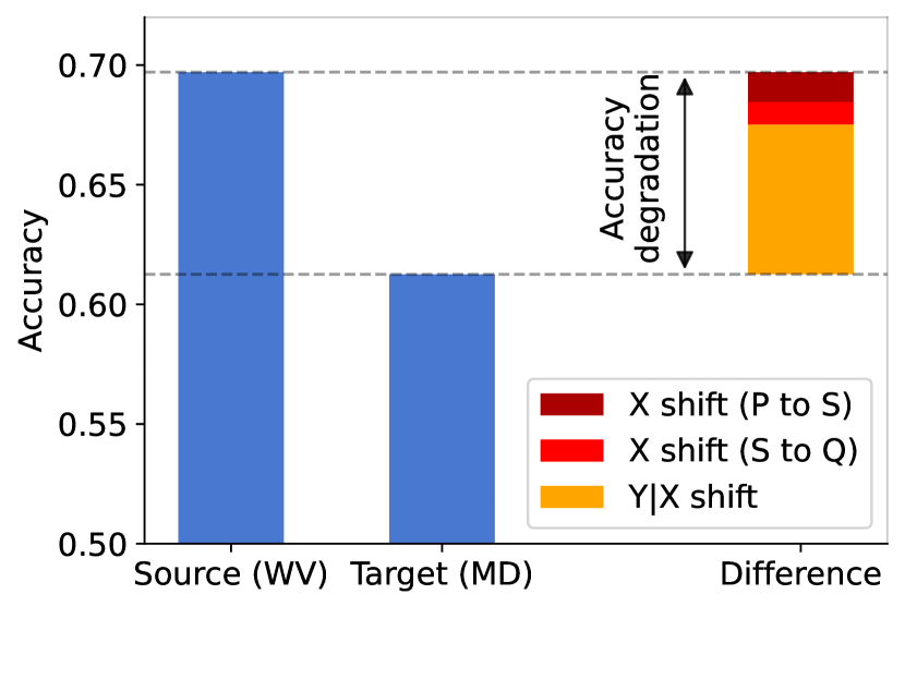
Figure 3: $Y\mid X$ shift: original model trained on West Virginia and evaluated on Maryland

Due to the cost of collecting and labeling enough data, it may be challenging to train a new model from scratch for each target site. Consider a prediction model trained on data collected from one site (West Virginia), which may be applied to other target sites (Maryland). To construct a specific type of $Y\mid X$ shift between sites, we consider a scenario where the initial feature set in the training data did not include educational attainment data. People in Maryland tend to be more educated than people in West Virginia, and educational attainment affects employment. Consequently, when educational attainment is not included in $X$, a $Y\mid X$ shift arises from marginalizing out the effect of education over a different distribution in West Virginia versus Maryland.

Let us now take the perspective of a modeler who did not know how this distribution shift was constructed. In Figure 3, observe that the prediction model trained in West Virginia performs worse in Maryland than in West Virginia; our goal is to understand this difference in performance. The decomposition depicted in the figure attributes substantial loss to a $Y\mid X$ shift. In response to such a decomposition, one might consider reasons why there is a $Y\mid X$ shift, including the possibility of a shift in the distribution of important unobserved variables. Analysts could use domain knowledge to consider educational attainment as one such unobserved variable, and obtain and append this feature to the original training set. Notably, collecting more features can often be less costly than collecting enough data from Maryland to fit a new model, and has the additional benefit of improving the model accuracy overall. Indeed, when we fit a new model on West Virginia incorporating educational attainment, we find that the new model performs well on both West Virginia and on Maryland, with an accuracy of 70% on Maryland, which is an improvement over the previous 61%.

4.1.2 $X$ shift: selection bias in age

Data can often be collected with unrecognized selection bias. Here, we consider a data collection process that oversamples people up to the age of 25 (e.g. from sampling near a college campus). We expect that it is easier to predict whether people of age $\leq 25$ are employed, as most of them are still in school. In contrast, older adults may encounter new situations that affect employment. Let us take the perspective of a modeler who notices that there is a difference between the training data and the general population (target $Q$) after the model is trained, and who obtains a carefully collected dataset over the general population for evaluation purposes. We demonstrate our approach on two training distributions that differ in their magnitude of selection bias and illustrate how the $X$ shift terms in the decomposition (2.1) can reflect such differences, and consequently inform future modeling interventions.

We first focus on the extreme case where the training data only consists of people of up to age 25. In Figure 4(a), the trained model performs much worse on the general population, and our decomposition correctly reveals that the decrease in performance is due to a $X$ shift. The performance degradation is primarily attributed to $X$ shift ($S\to Q$), indicating that the model performed poorly on examples in the general population ($Q$) that were rarely encountered during training. To better understand the shift from $P_{X}$ to $Q_{X}$, we use the feature importance method for random forests [70] on the domain classifier and find that the most important feature, as expected, is age. Our method thus suggests that data collection over an older population may be necessary in order to perform well on the general population. Indeed, a new employment model fitted on more samples from all ages has an improved target accuracy of 73%, compared to the original model’s target accuracy of 66%.

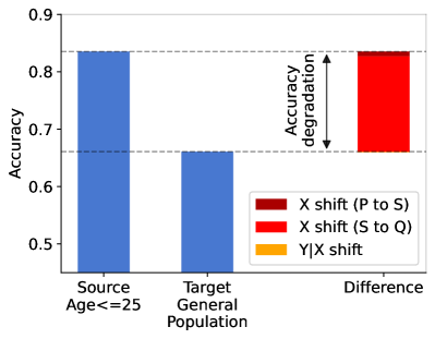
(a)

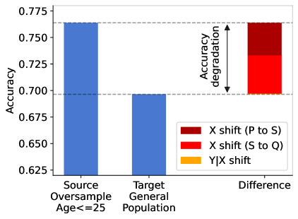
(b)

Figure 4: Moderate vs. severe $X$-shift. Both models are evaluated on the general population.

Next, we consider a less dramatic shift in the distribution of $X$, where people up to the age of $25$ are merely overrepresented in the training data. In Figure 4(b), we observe that the model performs worse on the general population as before, and our decomposition again reveals that the decrease in performance is primarily attributed to an $X$ shift. Unlike in the previous example, the training data here includes people of all ages, and we see that the $X$ shift ($P\to S$) term is larger as a result. This suggests that instead of resorting to an expensive data collection process, reweighting the original dataset may be an effective algorithmic solution to adapt to the target. We fit a new model on an appropriately re-weighted version of the original training data and find that the new model achieves an accuracy of 80% on the target, a significant improvement over the previous model’s target accuracy of 69%.

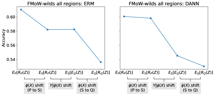
Figure 5: ERM (left) vs DANN (right) in the distribution shift from FMoW-wilds. On the vertical axis is model accuracy; all results hold using accuracy in place of $\ell(\cdot)$. On the horizontal axis are the four values in Equation (2.4). Their consecutive differences are the $Z=\phi(X)$ shift ($P\to S$), $Y\mid\phi(X)$ shift, and $\phi(X)$ shift ($S\to Q$) terms, respectively. Both ERM and DANN perform worse on target than training, and DANN is not better on target data compared to ERM. For ERM, the $\phi(X)$ shift terms are largest; for DANN, the $Y\mid\phi(X)$ terms are largest.

4.2 Diagnosing failures of domain-adaptation methods

We study an image classification problem where the learned feature representation plays a critical role in the distributional robustness of a prediction model. We focus on satellite image classification, which can inform humanitarian and sustainability efforts by tracking deforestation, population density, and other economic metrics [81]. In order to track these metrics effectively, such models must perform reliably over space and time. We consider a spatio-temporal distribution shift for classifying land use from satellite images on a variant of the Functional Map of the World dataset [81], called FMoW-wilds [19]. The training data consists of images before 2013, while the target data is from 2016 and after, and the proportion of samples from different geographical regions is different between training and target.

Sagawa et al. [81] recently observed that classifiers trained via the standard empirical risk minimization (ERM) approach (also known as sample average approximation) perform significantly worse on the target distribution compared to training. They also noted that algorithmic interventions do not, in fact, provide meaningful robustness gains over ERM. To illustrate how these methods can fail, we focus on a specific domain adaptation method, called Domain Adversarial Neural Network (DANN) [34]. The main idea of DANN is to learn a feature embedding $\phi(X)$ of $X$ such that the distribution of $\phi(X)$ is difficult to distinguish between training and target. Specifically, DANN uses labeled $(X,Y)$ data from training and unlabeled $X$ data from target to learn neural network feature representations $\phi(X)$ that are not only useful for predicting $Y$ on the training data, but are also difficult to classify as being from training vs target. Intuitively, requiring $\phi(X)$ to be difficult to classify as being from either distribution can reduce $\phi(X)$ shift, and thus also loss attributed to $\phi(X)$ shift.

We investigate why models trained using DANN perform poorly on the target, even though DANN was designed to perform well across a distribution shift. Using the output of the penultimate layer of the neural network as features so that $Z_{\rm ERM}=\phi_{\rm ERM}(X)$ and $Z_{\rm DANN}=\phi_{\rm DANN}(X)$ for the respective models, we fit $\hat{\pi}$ using a logistic regression and present our decomposition (2.4) in Figure 5. Compared to the ERM model, the DANN counterpart has less performance degradation attributed to $\phi(X)$ shift. However, the performance degradation attributed to $Y\mid\phi(X)$ is much larger for the DANN model, so that DANN performs poorly overall, even though it successfully has less performance degradation attributed to $\phi(X)$ shift. Such a performance degradation can occur if the assumption that the distributions of $\phi(X)$ should be indistinguishable between train and target is inappropriate. This trade-off between different types of distribution shifts highlights the pitfalls of solely focusing on protecting against $\phi(X)$-shifts, as is common practice in domain adaptation. See Section 5 for confidence intervals.

5 Statistical properties

In this section, we study the statistical properties of the estimators $\hat{\theta}_{P},\;\hat{\theta}_{Q}$ (3.9), and the estimators for the decomposition terms from Equation (2.1) from Algorithm 1. We show asymptotic normality, efficiency, and the validity of bootstrapping methods for estimating confidence intervals. Then, we apply our statistical guarantees to calculate confidence intervals for the experiments in Section 4.

We give conditions under which we know that $\hat{\theta}_{P},\;\hat{\theta}_{Q}$, and the estimators for the decomposition terms from Equation (2.1) from Algorithm 1 are asymptotically normal. Knowing the asymptotic distribution allows us construct confidence intervals for the true parameters $\theta_{P},\;\theta_{Q}$, and the decomposition terms from Equation (2.1). In Appendix C, we use heuristics developed by Kennedy [48] to show that our estimator is asymptotically efficient, suggesting that our estimator cannot be improved upon in terms of asymptotic variance.

Recall our notation from Section 3

$$\begin{split}&\alpha^{*}~{}~{}\mbox{is the proportion of the pooled data that comes from}~{}Q_{X}\\ &T=\begin{cases}0~{}~{}&\mbox{if}~{}\tilde{X}~{}\mbox{is from}~{}P_{X}\\ 1~{}~{}&\mbox{if}~{}\tilde{X}~{}\mbox{is from}~{}Q_{X}\end{cases}\\ &\pi^{*}(x)\mathrel{\mathop{\mathchar 58\relax}}=\mathbb{P}(T=1\mid\tilde{X}=x)=\frac{\alpha^{*}q(x)}{\alpha^{*}q(x)+(1-\alpha^{*})p(x)}\end{split}$$

The statistical behavior of $\hat{\theta}_{P},\;\hat{\theta}_{Q},$ and the estimators for the decomposition terms from Equation (2.1) depend on the estimator $\hat{\pi}(x)$ used for the nuisance parameter $\pi^{*}(x)$. However, as is the case for many other semiparametric estimators, when the nuisance parameter estimates converge sufficiently quickly and smoothly, the asymptotic distributions of $\hat{\theta}_{P}$ and $\hat{\theta}_{Q}$ are well-approximated in a way that does not depend on the form of the nuisance parameter estimator [64]. In particular, the nuisance parameters need not be estimated at the $\sqrt{n}$-rate for $\hat{\theta}_{P},\;\hat{\theta}_{Q}$ to be asymptotically normal at the $\sqrt{n}$-rate. We show asymptotic normality of the main estimators when the nuisance parameter $\pi^{*}(\cdot)$ can only be estimated at the $n^{1/4}$-rate. Key to this, however, is “undersmoothing” of the nuisance parameters [66], as we describe below.

In this section, we focus on understanding the approximation when the nuisance parameter is estimated using nonparametric kernel smoothing. Kernel smoothing is a well-established nonparametric estimation technique [66], where the prediction for a test point $x$ is a locally-weighted average of the outcomes for observations “near” $x$ in the training data. The weighting is defined by a kernel function $K(\cdot)$ and a bandwidth $\sigma>0$, and the weighting is done using $K_{\sigma}(t)\mathrel{\mathop{\mathchar 58\relax}}=\sigma^{-1}K(t/\sigma)$. Applying this approach to estimate $\pi^{*}(\cdot)$ gives

$$\hat{\pi}(x)=\frac{\frac{1}{n}\sum_{i=1}^{n}T_{i}K_{\sigma}(x-X_{i})}{\frac{1}{n}\sum_{i=1}^{n}K_{\sigma}(x-X_{i})}.$$

While other estimators will give similar results under different assumptions about the data generating process, focusing on this one allows us to take advantage of existing technical results for kernel smoothing and to focus our attention on the behavior of the semiparametric estimators themselves.

We write the kernel smoothing estimate $\hat{\pi}(\cdot)$ as the ratio of two kernel density estimators: let $A=[1,T]^{\top}$ and

$$\hat{\gamma}(x) =\frac{1}{n}\sum_{i=1}^{n}AK_{\sigma}(x-X_{i})$$ (5.1)

so that $\hat{\gamma}$ is an estimator for the true $\gamma^{*}$ with $\gamma_{j}^{*}(x)\mathrel{\mathop{\mathchar 58\relax}}=m_{X}(x)\mathbb{E}[A_{j}\mid X=x]$, with $\gamma_{1}^{*}(x)=m_{X}(x)$ the marginal density of $z$ across the pooled data from $P$ and $Q$, and $\gamma_{2}^{*}(x)=m_{X}(x)\mathbb{E}[T\mid X=x]$. Then $\hat{\pi}(x)=\hat{\gamma}_{2}(x)/\hat{\gamma}_{1}(x)$.

To get good rates of convergence, we need to be careful with choosing the kernel and bandwidth.

Assumption A (Kernel density estimator assumptions).

Let $d$ be the dimension of $X$. For some choice of constants $k$ and $p$,

1. $K(u)$ is differentiable of order $p$, the derivatives of order $p$ are bounded, $K(u)$ is zero outside of a bounded set, $\int K(u)du=1$, there is a positive integer $k$ such that for all $j<k$, $\int K(u)[\bigotimes_{l=1}^{j}u]du=0$.

2. The bandwidth $\sigma=\sigma(n)$ satisfies $n\sigma^{2d+4p}/(\ln n)^{2}\to\infty$ and $n\sigma^{2k}\to 0$.

Remark 1.

If the bandwidth $\sigma=\sigma(n)=n^{b}$, then for Assumption A to hold, we would need

$$-\frac{1}{2r+4d}<b<-\frac{1}{2k}.$$

This requires the bandwidth to shrink faster than the rate used to get minimax optimal convergence of the nuisance parameters themselves with kernel smoothing [90, 66]. As a result, the pointwise variance of the nuisance parameter estimates will be higher, and the bias will be lower. This turns out to be critical for getting $\sqrt{n}$-consistency of the semiparametric estimators $\hat{\theta}_{Q}$ and $\hat{\theta}_{P}$, and is one widely applicable lesson that applies broadly to most applicable methods for nuisance parameter estimation in our setting. Therefore, we recommend users to choose hyperparameters that lead to mild, yet notiable undersmoothing when fitting nuisance parameters for our method. Unfortunately, reliable methods for automatically choosing hyperparameters to achieve these requirements are currently not well-known in the literature.

To ensure that the estimates from nonparametric kernel smoothing converge sufficiently quickly over the entire domain, we additionally make the following assumptions.

Assumption B.

1. $X$ has support on a compact set $\mathcal{X}$, on which its density $m_{X}(x)$ is bounded above and below (away from 0): there are $B_{mL}>0$ and $B_{mU}<\infty$ such that $B_{mL}<m_{X}(x)<B_{mU}$ for all $x$.

2. $\pi^{*}(x)\mathrel{\mathop{\mathchar 58\relax}}=\mathbb{P}(T=1\mid X=x)$ is bounded away from 0 and 1: there is a $\delta_{\pi}>0$ such that $0<\delta_{\pi}<\pi^{*}(x)<1-\delta_{\pi}<1$ for almost every $x$.

3. $\pi^{*}(x)$ is continuous almost everywhere.

4. There is a version of $\gamma^{*}(x)$ that is continuously differentiable to order $p$ with bounded derivatives on an open set containing $\mathcal{X}$.

Assumptions like these are standard for kernel smoothing estimators [66, 99], and are necessary to ensure convergence over the entire domain.

With these assumptions, the nuisance parameters will not typically be estimated at the parametric $\sqrt{n}$ rate. However, when plugged into our semiparametric method, the overall estimators $\hat{\theta}_{P}$ and $\hat{\theta}_{Q}$ will converge at a $\sqrt{n}$ rate, and be asymptotically normal, so long as the loss $L=\ell(f(X),Y)$ is sufficiently regular. We describe sufficient regularity conditions for $L$ in the assumption below.

Assumption C.

1. $\mathbb{E}[L^{4}]<B_{L^{4}}$ for some $B_{L^{4}}<\infty$.

2. $\mu_{Q}(x)\mathrel{\mathop{\mathchar 58\relax}}=\mathbb{E}[L\mid T=1,X=x]$ and $\mu_{P}(x)\mathrel{\mathop{\mathchar 58\relax}}=\mathbb{E}[L\mid T=0,X=x]$ are continuous almost everywhere.

3. $\mu_{Q}(x),\mu_{P}(x)<B_{\mu}<\infty$ for some $B_{\mu}$ on $\mathcal{X}$.

Because our estimators (3.9) depend on the product of functions of $\hat{\pi}(\cdot)$ and the loss $L$, Assumption C ensures that small estimation errors in $\hat{\pi}(\cdot)$ aren’t amplified in pathological ways when multiplied by $L$. With these three assumptions, our estimators are jointly regular and asymptotically linear. Our main result (Theorem 2 to come) makes precise the asymptotic distribution of the estimator $\hat{\theta}_{Q}$. A symmetric result holds for $\hat{\theta}_{P}$, and from these we can deduce the asymptotic distribution of the decomposition terms in Equation (2.1).

To state Theorem 2, we introduce additional notation. Building on Equation (3.4), let $M(\cdot)$ denote the distribution of the observed data. Let $M_{X}(\cdot)$ be the marginal distribution of $X$ under this distribution, and $m_{X}(x)$ its density. As before, define $T$ as a binary dummy variable that is $1$ when the observation comes from the target distribution $Q$ and $0$ when it comes from the training distribution $P$. Then as in Section 3 we can write

$$\theta_{Q}=\mathbb{E}_{M}\left[\frac{\operatorname{d\!}{S_{X}}}{\operatorname{d\!}{M_{X}}}\frac{\mathbf{1}\left\{T=1\right\}}{\mathbb{P}_{M}(T=1\mid X)}L\right]~{}~{}\mbox{ and }~{}~{}\theta_{P}=\mathbb{E}_{M}\left[\frac{\operatorname{d\!}{S_{X}}}{\operatorname{d\!}{M_{X}}}\frac{\mathbf{1}\left\{T=0\right\}}{\mathbb{P}_{M}(T=0\mid X)}L\right].$$

Recalling that $\pi^{*}(x)\mathrel{\mathop{\mathchar 58\relax}}=\mathbb{P}_{M}(T=1\mid X=x)$, and using Equation (2.2) and some calculations,

$$\frac{\operatorname{d\!}S_{X}}{\operatorname{d\!}M_{X}}\propto\lambda(\pi^{*}(X),\alpha^{*})~{}~{}\text{ where}~{}~{}\lambda(\pi,\alpha)=\frac{\pi(1-\pi)}{(1-\alpha)\pi+\alpha(1-\pi)}.$$ (5.2)

Then we can write our estimands $\theta_{P}$, $\theta_{Q}$ as functionals of the data distribution $M$, the conditional probability $\pi^{*}(X)$, and the marginal probability $\alpha^{*}=\mathbb{P}_{M}(T=1)$ as

$$\theta_{P}=\frac{\mathbb{E}_{M}\left[L\frac{1-T}{1-\pi^{*}(X)}\lambda(\pi^{*}(X),\alpha^{*})\right]}{\mathbb{E}_{M}\left[\frac{1-T}{1-\pi^{*}(X)}\lambda(\pi^{*}(X),\alpha^{*})\right]}~{}~{}~{}\mbox{and}~{}~{}~{}\theta_{Q}=\frac{\mathbb{E}_{M}\left[L\frac{T}{\pi^{*}(X)}\lambda(\pi^{*}(X),\alpha^{*})\right]}{\mathbb{E}_{M}\left[\frac{T}{\pi^{*}(X)}\lambda(\pi^{*}(X),\alpha^{*})\right]}.$$ (5.3)

For brevity, let $W$ denote $(X,T,L)$. Then we show the asymptotic linearity of $\hat{\theta}_{Q}$:

Theorem 2.

Let $\hat{\gamma}$ be as in Equation (5.1). Then, under Assumptions A, B, and C,

$$\sqrt{n}(\hat{\theta}_{Q}-\theta_{Q})=\sum_{i=1}^{n}\psi_{Q}(w_{i})/\sqrt{n}+o_{P}(1),$$

so that

$$\sqrt{n}(\hat{\theta}_{Q}-\theta_{Q})\stackrel{{\scriptstyle d}}{{\rightsquigarrow}}N(0,{\rm Var}(\psi_{Q}(W))).$$

where

$$\psi_{Q}(w)=\left(\mathbb{E}\left[\frac{T}{\pi^{*}(X)}\lambda(\pi^{*}(X),\alpha^{*})\right]\right)^{-1} \Bigg{\{}(l-\theta_{Q})\frac{t}{\pi^{*}(x)}\lambda(\pi^{*}(x),\alpha^{*})$$

$$\hskip 10.00002pt+\mathbb{E}\left[(L-\theta_{Q})\frac{T}{\pi^{*}(X)}\frac{\partial}{\partial\alpha}\lambda(\pi^{*}(X),\alpha)\Big{|}_{\alpha=\alpha^{*}}\right](t-\alpha^{*})$$

$$\hskip 10.00002pt+(\mu_{Q}(x)-\theta_{Q})\pi^{*}(x)(t-\pi^{*}(x))\frac{\partial}{\partial\pi}\left[\frac{\lambda(\pi,\alpha^{*})}{\pi}\right]\Big{|}_{\pi=\pi^{*}(x)}\Bigg{\}}$$

See Appendix A for the proof. An analogous result holds for $\hat{\theta}_{P}$, and the decomposition terms from Equation (2.1) follows immediately as $\hat{\theta}_{P},\;\hat{\theta}_{Q}$ are asymptotically linear. Theorem 2 can be further generalized: Yadlowsky [104] shows that the assumptions needed to guarantee asymptotic linearity with the same influence function extend immediately to cross-fitted analogues of these estimators (see Appendix D.1 for more on cross-fitting). Additionally, the literature has many results showing asymptotic linearity of semiparametric methods using other nuisance parameter estimators under more general conditions than those assumed in the proofs provided here [65, 18]. This is because many of these results have a similar form, with the first order effect of estimating the nuisance parameters is the influence function in Theorem 2, and the remaining error terms that depend on the specific choice of nuisance parameter estimator are lower order. See, for example, Newey [64, 65], Kennedy [48], Yadlowsky [104].

The asymptotic linearity in our result directly ensures that subsampling procedures such as half-sampling [20] are justified for constructing calibrated confidence intervals. The half-sample bootstrap [29, 72] is a simple procedure of this form, which Yadlowsky et al. [105, Lemma 4] showed directly applies here (Corollary 1). The half-sample bootstrap is constructed by repeatedly drawing samples of half the data without replacement, constructing the estimator $\hat{\theta}_{Q}^{\ast}$ with each sample, and analyzing the distribution of the errors $\hat{\theta}_{Q}^{\ast}-\hat{\theta}_{Q}$. Our next result shows that this provides be a good approximation of the sampling distribution of $\hat{\theta}_{Q}-\theta_{Q}$. In this corollary (of Yadlowsky et al. [105, Lemma 4]), $P^{\ast}$ refers to the observed Monte Carlo distribution of the procedure, and is conditional on the observed data (and therefore, $\hat{\theta}_{Q}$).

Corollary 1.

Under the conditions of Theorem 2, conditionally on the observed data, the Monte Carlo distribution of $\sqrt{n}(\hat{\theta}_{Q}^{\ast}-\hat{\theta}_{Q})\overset{P^{\ast}}{\to}N(0,{\rm Var}(\psi_{Q}(W)))$.

Confidence intervals in practice

Showing that the nonparametric bootstrap [29] gives valid confidence intervals requires additional work. However, given the regularity of our functional, we conjecture that the nonparametric bootstrap also provides calibrated confidence intervals. The advantage of the nonparametric bootstrap is its simplicity and reduced sensitivity to finite sample defects resulting from each subsample being larger in size. In this subsection, we empirically verify that the nonparametric bootstrap provides similar inference to the theoretically-justified half-sample bootstrap, so we recommend this procedure for routine practice.

		Standard error
Term	Estimate	NP boot	HS boot	IF est
$X$ shift ($P\to S$)	0.78%	0.66%	0.71%	0.96%
$Y\mid X$ shift	6.29%	0.97%	1.17%	1.13%
$X$ shift ($S\to Q$)	1.35%	0.68%	0.75%	0.86%

(a) $Y|X$ shift: original model trained on West Virginia and evaluated on Maryland

		Standard error
Term	Estimate	NP boot	HS boot	IF est
$X$ shift ($P\to S$)	0.23%	0.38%	0.43%	0.53%
$Y\mid X$ shift	-0.01%	0.43%	0.53%	0.56%
$X$ shift ($S\to Q$)	17.21%	0.33%	0.34%	0.40%

(b) $X$ shift: model trained on only age $\leq$25 and evaluated on general population

		Standard error
Term	Estimate	NP boot	HS boot	IF est
$X$ shift ($P\to S$)	2.03%	0.79%	0.67%	1.13%
$Y\mid X$ shift	0.27%	0.97%	1.05%	1.26%
$X$ shift ($S\to Q$)	5.15%	0.64%	0.63%	0.89%

(c) $X$ shift: model trained on over-sampling age $\leq$25 and evaluated on general population

Table 2: Point estimate and estimates of standard error for estimators of decomposition terms for Section 4.1. The standard error column names are abbreviated: “NP boot” is short for nonparametric boostrap and “HS boot” is short for half-sample bootstrap, as described in Section 5. Each type of bootstrapping is done with 500 bootstrap re-samples. “IF est” is short for plug-in estimator of influence function: we calculate the standard error using influence functions as in results like Theorem 2 and plug in estimates $\hat{\pi}(x),\hat{\mu}_{Q}(x),\hat{\alpha}$ in place of $\pi^{*}(x),\mu_{Q}(x),\alpha^{*}$.

In Table 2, we first compare different ways of calculating confidence intervals for Section 4.1 using methods from Section 5. Next, we calculate nonparametric bootstrap confidence intervals for Section 4.2. The confidence intervals in Table 3 show that the conclusions drawn from our previous analysis are not due to happenstance and are statistically sound.

	ERM			DANN
Term	Estimate	NP boot SE		Estimate	NP Boot SE
$\phi(X)$ shift ($P\to S$)	2.82%	0.15%		0.25%	0.13%
$Y\mid\phi(X)$ shift	-0.04%	0.40%		5.29%	0.40%
$\phi(X)$ shift ($S\to Q$)	4.62%	0.15%		1.49%	0.13%

Table 3: Estimates for ERM vs DANN, corresponding to Figure 5. The standard errors are calculated using non-parametric bootstrap with 100 bootstrap samples (“NP boot SE”)

6 Discussion

Distribution shift is a fundamental problem in data-driven decision-making. Still, there are limited tools for understanding changes in model performance with respect to different types of distribution shifts. We introduce a simple method, DIstribution Shift DEcomposition (DISDE) that can diagnose out-of-distribution performance by attributing the change in loss to three terms, corresponding to 1) an increase in harder but frequently seen examples from training, 2) changes in the relationship between features and outcomes, and 3) poor performance on examples infrequent or unseen during training (Sections 2, 3). We empirically demonstrate how DISDE can inform modeling improvements on tabular and image data (Section 4), and we analyze its asymptotic properties (Section 5). In this final section, we situate the current work in the large body of literature on distribution shifts (Section 6.1) and discuss the limitations of our approach alongside future research directions (Section 6.2).

6.1 Related work

Distribution shift is an important topic across multiple research communities. Much of the work is on training better models through methodological improvements. Like ours, some works focus on taxonomies for discussing distribution shifts [58, 84, 97]. Complementary to our work, other works focus on collecting data across distribution shifts. However, there is not much research on attributing changes in model performance to different types of distribution shifts. Concurrent to our work, Zhang et al. [108] use Shapley value to attribute changes in performance to various types of shift, but do not address differences in support or density between distributions as we do with the shared distribution in DISDE (Section 2).

In the machine learning community, domain adaptation methods train models using data from a training distribution, and aim to perform well on a specified target distribution. Standard approaches assume the $Y\mid X$ distribution is fixed and reweight training data to resemble the target distribution [87, 41, 11, 92, 98]. When we expect shifts in the $Y\mid X$ distribution, Meinshausen and Bühlmann [59], Rothenhäusler et al. [79] propose learning models that have good performance against causal interventions that affect $Y\mid X$. More recently, several authors have studied approaches that aim to learn feature representations $\phi(X)$ such that $Y\mid\phi(X)$, or functionals thereof, is invariant across multiple environments [71, 80, 2, 78].

There is a large body of work on distributionally robust optimization (DRO) methods that optimize performance over distributions that are “close” to the training distribution. While the majority of these works consider shifts in the joint distribution $(X,Y)$ [31, 25, 103, 8, 53, 63, 9, 52, 89, 9, 100, 28], some notions of closeness (e.g., Wasserstein distance) can flexibly handle both joint and covariate shifts [85, 12, 35, 13, 51]. Despite the extensive literature on DRO, limited work study particular types of distribution shifts. Focusing on the case of covariate shifts, Duchi et al. [27] develop tailored methods that optimize worst-case subpopulation shifts over a set of covariates. Similarly, Sahoo et al. [82] propose a related worst-case subpopulation formulation over $Y\mid X$-shifts, holding the marginal distribution of $X$ fixed.

The causal inference community takes a more nuanced approach to distribution shift. There is extensive work on sensitivity analysis (e.g., [76, 77, 46, 33, 47, 106]), which studies the amount of unobserved confounding—analogous to the magnitude of $Y\mid X$ shift in predictive scenarios—to call into question the conclusion of observational studies. When a known target population differs from the study population, a large body of research adjusts observations to resemble the target [91, 94, 49, 56]. These approaches are analogous to domain adaptation under covariate shift; analogous to distributionally robust optimization, Jeong and Namkoong [45] recently formulate worst-case sensitivity approaches for covariate shift. More generally, the external validity of a study can be called into question due to different distribution shifts. Egami and Hartman [30] formalize and contextualize the type of shifts that naturally arise in social sciences.

Our approach complements design-based and benchmarking research in statistics and machine learning. Collecting maximally heterogeneous data is a classical idea in experimental design, with a recent focus on multi-site designs [22, 5, 36, 24, 96, 95]. In machine learning, building on older literature on distribution shifts [38, 74], there is renewed interest in benchmarking model performance on unseen test distributions different from training [75, 50, 39, 60]. For example,  Recht et al. [75], Taori et al. [93] observe a trend in which models trained on the same data universally suffer a relative performance degradation on new distributions, regardless of the training method and model capacity. By evaluating model robustness over multiple distributions, these works spur empirical progress by simulating typical ML deployment processes where models encounter a priori unknown distributions under operation. While out-of-distribution benchmarks and industrial monitoring systems primarily focus on detecting performance degradation [42], we build a diagnostic that generates qualitative insights on the cause of the observed failure. We hope this work provides a starting point for building a principled language for understanding performance degradation over distribution shifts.

6.2 Limitations and future work

Our work has several limitations, some of which are by design. For example, by design, DISDE does not directly propose new interventions; it is a diagnostic that can help decide between potential interventions, or to help assess existing interventions. In addition, DISDE only applies in certain settings: for now, it only concerns shifts between pairs of distributions, and not among more distributions. It also only applies to losses that can be written as $\mathbb{E}[\ell(f(X),Y)]$. Therefore, it does not directly apply to an F1-score or a worst-subgroup loss, for example. Lastly, our work assumes the existence of a shared distribution $S_{X}$ (Section 2). If there is no shared support between $P_{X}$ and $Q_{X}$, then our decomposition will not be valid.

Other limitations of our approach concern the limitations of the work that it builds on. In particular, our methodology involves an auxiliary domain classifier, which is analogous to the propensity score in causal inference. How best to learn a propensity score is a field of active research. For example, there are questions on the role of balancing covariates between treatment and control, versus modeling treatment assignment [43, 109, 15]. In our work we use a very simple way to learn a propensity score and leave extensions to future work.

Broadly speaking, our work highlights the potential benefits of an operations engineering approach to the training, deployment, and use of machine learning models. Classical quality control and reliability engineering methods have had major impacts across multiple industries (e.g., car manufacturing [73], electronics manufacturing [62], software development processes [69]). As the use of ML models becomes increasingly prevalent and complex, we will need ways to diagnose model failures and to direct resources to the appropriate modeling interventions. However, currently, even the most advanced industrial monitoring systems can only detect performance degradation, without attribution to its cause [42]. We hope this paper spurs further work to build rigorous and scalable tools for the quality management of ML applications. For example, to analyze the local sensitivity of a simulation output, several authors have used conditional variances to attribute variance due to different subsets of the input [40, 83, 67, 88] and related approaches may yield fruit in the context of ML models.

7 Acknowledgements

Tiffany Cai is supported by the National Science Foundation Graduate Research Fellowship under Grant No. DGE-2036197. Hongseok Namkoong was partially supported by the Amazon Research Award.

Appendix A Proofs for asymptotic properties for the estimator

In this section, we will prove Theorem 2, to show the asymptotically linear expansion of $\hat{\theta}_{Q}$. Recalling the definition of $\theta_{Q}$ (5.3), denote by $D_{Q}$ and $N_{Q}$ the denominator and the numerator

$$D_{Q}=\mathbb{E}\left[\frac{T}{\pi^{\star}(X)}\lambda(\pi^{\star}(X),\alpha^{\star})\right]~{}~{}~{}\text{and}~{}~{}~{}N_{Q}=\mathbb{E}\left[L\frac{T}{\pi^{\star}(X)}\lambda(\pi^{\star}(X),\alpha^{\star})\right].$$

Observe that the numerator and denominator of $\theta_{Q}$ (and also $\hat{\theta}_{Q}$) are nearly identical: we can think of the denominator $D_{Q}$ (and its empirical plug-in $\widehat{D}_{Q}$) as a special case of the numerator $N_{Q}$ (and also $\hat{N}_{Q}$) but with $L\mathrel{\mathop{\mathchar 58\relax}}=1$. Below, we focus on asymptotic expansions for $N_{Q}$ without loss of generality.

The following lemma shows it suffices to find the asymptotically linear expansion of the numerator and denominator of $\hat{\theta}_{Q}$ separately. We defer its proof to Section B.1.

Lemma 1.

Assume that $A_{n}\stackrel{{\scriptstyle p}}{{\rightarrow}}A$, $B_{n}\stackrel{{\scriptstyle p}}{{\rightarrow}}B$, $\sqrt{n}(A_{n}-A)=\frac{1}{\sqrt{n}}\sum_{i=1}^{n}a_{i}+o_{P}(1)$ and $\sqrt{n}(B_{n}-B)=\frac{1}{\sqrt{n}}\sum_{i=1}^{n}b_{i}+o_{P}(1)$. Additionally, assume that $B>0$. Then,

$$\sqrt{n}\left(\frac{A_{n}}{B_{n}}-\frac{A}{B}\right)=\frac{1}{\sqrt{n}}\sum_{i=1}^{n}\left(\frac{1}{B}a_{i}-\frac{A}{B^{2}}b_{i}\right)+o_{P}(1).$$

Because of Lemma 1, it suffices to prove the following proposition; we give its proof in the rest of this section. Let $\widehat{N}_{Q}$ be the empirical plug-in for $N_{Q}$

$$\widehat{N}_{Q}\mathrel{\mathop{\mathchar 58\relax}}=\sum_{i=1}^{n}l_{i}\frac{t_{i}}{\hat{\pi}(x_{i})}\lambda(\hat{\pi}(x_{i}),\hat{\alpha}).$$ (A.1)

Proposition 3.

$\sqrt{n}(\hat{N}_{Q}-N_{Q})=\frac{1}{\sqrt{n}}\sum_{i=1}^{n}\psi_{N_{Q}}(w_{i})+o_{P}(1)$, where $\psi_{N_{Q}}(w)=g(w)+h(w)+\delta(w)$ and

$$g(w) =l\frac{t}{\pi^{*}(x)}\lambda(\pi^{*}(x),\alpha^{*})-N_{Q}$$

$$h(w) =\mathbb{E}\left[L\frac{T}{\pi^{*}(X)}\frac{\partial}{\partial\alpha}\lambda(\pi^{*}(X),\alpha)\Big{|}_{\alpha=\alpha^{*}}\right](t-\alpha^{*})$$

$$\delta(w) =\mu_{Q}(x)\pi^{*}(x)(t-\pi^{*}(x))\frac{\partial}{\partial\pi}\left[\frac{\lambda(\pi,\alpha^{*})}{\pi}\right]\Big{|}_{\pi=\pi^{*}(x)}.$$

To begin, recall that $\pi(x)=\gamma_{2}(x)/\gamma_{1}(x)$ and define

$$g(w,\gamma,\alpha) =l\frac{t}{\pi(x)}\lambda(\pi(x),\alpha)-N_{Q}$$ (A.2)

so that

$$\widehat{N}_{Q}-N_{Q}=n^{-1}\sum_{i=1}^{n}g(w_{i},\hat{\gamma},\hat{\alpha}).$$

Since $g$ is continuously differentiable with respect to $\alpha$, expand $\hat{\alpha}$ around $\alpha^{*}$ as

$$g(w_{i},\hat{\gamma},\hat{\alpha}) =\nabla_{\alpha}g(w_{i},\hat{\gamma},\overline{\alpha})(\hat{\alpha}-\alpha^{*})+g(w_{i},\hat{\gamma},\alpha^{*})$$

where $\overline{\alpha}$ is a mean value. By Lemma 2 below, $n^{-1}\sum_{i=1}^{n}\nabla_{\alpha}g(w,\hat{\gamma},\alpha)\stackrel{{\scriptstyle p}}{{\rightarrow}}\mathbb{E}[\nabla_{\alpha}g(w,\gamma^{*},\alpha)].$

Lemma 2.

Under the assumptions and definitions of Theorem 2,

$$n^{-1}\sum_{i=1}^{n}\nabla_{\alpha}g(w,\hat{\gamma},\overline{\alpha})\stackrel{{\scriptstyle p}}{{\rightarrow}}\mathbb{E}[\nabla_{\alpha}g(w,\gamma^{*},\alpha^{*})]=\mathrel{\mathop{\mathchar 58\relax}}G_{\alpha}$$

Proof of this lemma is deferred to Section B.2. Noting that $\hat{\alpha}=n^{-1}\sum_{i=1}^{n}t_{i}$ and letting

$$h(w)\mathrel{\mathop{\mathchar 58\relax}}=\mathbb{E}[\nabla_{\alpha}g(w,\gamma^{*},\alpha^{*})](t-\alpha^{*})=\mathbb{E}\left[L\frac{T}{\pi^{*}(X)}\nabla_{\alpha}\lambda(\pi^{*}(X),\alpha^{*})\right](t-\alpha^{*}),$$

we arrive at

$$\sum_{i=1}^{n}g(w_{i},\hat{\gamma},\hat{\alpha})/\sqrt{n} =\sum_{i=1}^{n}[h(w_{i})+g(w_{i},\hat{\gamma},\alpha^{*})]/\sqrt{n}+o_{P}(1).$$ (A.3)

To find an asymptotically linear representation of $\sum_{i=1}^{n}g(w_{i},\hat{\gamma},\alpha^{*})/\sqrt{n},$ we will show that under the assumptions made in Theorem 2, $\sum_{i=1}^{n}g(w_{i},\hat{\gamma},\alpha^{*})/\sqrt{n}$ satisfies the assumptions of Newey and McFadden [66, Theorem 8.11], which we restate now for convenience. Note that while the theorem as stated in Newey and McFadden [66] only shows asymptotic normality, in the proof they show asymptotic linearity, so we have modified the result to state the asymptotic linearity result, instead. We have also modified the result for the case where $g$ is linear in the estimated parameter, in which case consistency of the estimated parameter does not need to be shown [66].

Assumption D (Newey and McFadden [66, Assumptions 8.1-8.3 and assumption from Theorem 8.11]).

Let $d$ be the dimension of $X$.

1. $K(u)$ is differentiable of order $p$, the derivatives of order $p$ are bounded, $K(u)$ is zero outside of a bounded set, $\int K(u)du=1$, there is a positive integer $m$ such that for all $j<m$, $\int K(u)[\bigotimes_{l=1}^{j}u]du=0$.

2. There is a version of $\gamma^{*}(x)$ that is continuously differentiable to order $p$ with bounded derivatives on an open set containing $\mathcal{X}$.

3. There is $r\geq 4$ such that $\mathbb{E}[\|A\|^{r}]<\infty$ and $\mathbb{E}[\|A\|^{r}|X=x]m_{X}(x)$ is bounded.

4. The bandwidth $\sigma=\sigma(n)$ satisfies $n\sigma^{2d+4p}/(\ln n)^{2}\to\infty$ and $n\sigma^{2m}\to 0$.

Assumption E (Newey and McFadden [66, assumptions from Theorem 8.11]).

Let $\beta$ be the parameter of interest, and $\hat{\beta}$ its estimator where $\hat{\beta}-\beta=\frac{1}{n}\sum_{i=1}^{n}g(W_{i},\hat{\gamma})$.

1. $\mathbb{E}[g(W,\gamma^{*})]=0$

2. $\mathbb{E}[\|g(W,\gamma^{*})\|^{2}]<\infty$

3. $\mathcal{X}$ is a compact set.

Assumption F (Newey and McFadden [66, enumerated assumptions from Theorem 8.11]).

There is a vector of functionals $G(w,\gamma)$ that is linear in $\gamma$ such that

1. for $\|\gamma-\gamma^{*}\|$ small where the norm is the Sobolev norm, $\|g(w,\gamma)-g(w,\gamma^{*})-G(w,\gamma-\gamma^{*})\|\leq b(w)\|\gamma-\gamma^{*}\|^{2}$, and $\mathbb{E}[b(W)]<\infty$;

2. $\|G(w,\gamma)\|\leq c(w)\|\gamma\|$ and $\mathbb{E}[c(W)^{2}]<\infty$;

3. there is $v(x)$ with $\int G(w,\gamma)dM(w)=\int v(x)\gamma(x)dx$ for all $\|\gamma\|<\infty$;

4. $v(x)$ is continuous almost everywhere, $\int\|v(x)\|dx<\infty$, and there is $\epsilon>0$ such that $\mathbb{E}[\sup_{\|\nu\|\leq\epsilon}\|v(X+\nu)\|^{4}]<\infty$.

Theorem 4 (N+M Theorem 8.11).

Let $\gamma^{*}$ be the nuisance parameter and $\hat{\gamma}$ its kernel density estimate satisfying Assumption D. Let $\beta$ be the parameter of interest, and $\hat{\beta}$ its estimator satisfying Assumption E. Assume there is a vector of functionals $G(w,\gamma)$ satisfying Assumption F. Then for $\delta(w)=v(x)a-\mathbb{E}[v(x)a]$,

$$\sum_{i=1}^{n}g(w_{i},\hat{\gamma})/\sqrt{n}=\sum_{i=1}^{n}[g(w_{i},\gamma^{*})+\delta(w_{i})]/\sqrt{n}+o_{P}(1).$$

We now proceed to use this result to prove the asymptotically linear representation

$$\sum_{i=1}^{n}g(w_{i},\hat{\gamma},\alpha^{*})/\sqrt{n} =\sum_{i=1}^{n}[g(w_{i},\gamma^{*},\alpha^{*})+\delta(w_{i})]/\sqrt{n}+o_{P}(1)$$ (A.4)

for our choice of $g(w,\gamma,\alpha)$. Then, the desired result follows from combining Equations (A.4) and (A.3), and then applying Lemma 1. What remains is to check the conditions of Theorem 4.

Verifying Assumption D:

1. Assumed in Assumption A

2. Assumed in Assumption B

3. There is $r\geq 4$ such that $\mathbb{E}[\|A\|^{r}]<\infty$ and $\mathbb{E}[\|A\|^{r}|X=x]m_{X}(x)$ is bounded: recall that $A=[1,T]$ and $T$ takes values in $\{0,1\}$. Then let $r=4$, $\|A\|^{r}\leq 2$, so that $\mathbb{E}[\|A\|^{r}]\leq 2<\infty$, and and $\mathbb{E}[\|A\|^{r}\mid X=x]m_{X}(x)\leq 2B_{mU}<\infty$ by Assumption B.

4. Assumed in Assumption A

Verifying Assumption E:

1. $\mathbb{E}[g(W,\gamma^{*},\alpha^{*})]=0$: this holds by definition of $g$ (Equation (A.2)) and $N_{Q}$ (Equation (A.1)).

2. $\mathbb{E}[|g(W,\gamma^{*},\alpha^{*})|^{2}]<\infty$:

   $$\mathbb{E}[|g(W,\gamma^{*},\alpha^{*})|^{2}] =\mathbb{E}\left[\left|L\frac{T}{\pi^{*}(X)}\lambda(\pi^{*}(X),\alpha^{*})-N_{Q}\right|^{2}\right].$$

   This is finite since $N_{Q}<\infty$, and then by Cauchy-Schwarz since $\mathbb{E}[L^{4}]<B_{L^{4}}$ by Assumption C, and $\left|\frac{T}{\pi^{*}(X)}\lambda(\pi^{*}(X),\alpha^{*})\right|^{4}$ is bounded, since $T\in\{0,1\}$ and

   $$\frac{\lambda(\pi^{*}(X),\alpha^{*})}{\pi^{*}(X)}=\frac{1-\pi^{*}(X)}{(1-\alpha^{*})\pi^{*}(X)+\alpha^{*}(1-\pi^{*}(X))}\leq\frac{1-\delta_{\pi}}{\delta_{\pi}}$$

   with $\delta_{\pi}$ from Assumption B.

3. Assumed in Assumption B.

Verifying Assumption F:

1. For $\|\gamma-\gamma^{*}\|$ small, $\left|g(w,\gamma,\alpha^{*})-g(w,\gamma^{*},\alpha^{*})-G(w,\gamma-\gamma^{*})\right|\leq b(w)\|\gamma-\gamma^{*}\|^{2}$, and $\mathbb{E}[b(W)]<\infty$: By Taylor-expanding $g$ around $\gamma^{*}(x)$ (where in the following equations we abuse notation and also use $g$ to mean $g(w,\gamma(x),\alpha)$, where the second argument is the value of the function $\gamma$ evaluated at $x$, rather than the function $\gamma$. We also write $\nabla_{\gamma}g(\cdot)$ to denote the derivative of this new $g$ with respect to its second argument, the value $\gamma(x)$, rather than to the function $\gamma(\cdot)$, and similarly for $\nabla^{2}_{\gamma}g(\cdot)$),

   $$g(w,\gamma,\alpha^{*}) =g(w,\gamma^{*}(x),\alpha^{*})+\nabla_{\gamma}g(w,\gamma^{*}(x),\alpha^{*})^{\top}(\gamma(x)-\gamma^{*}(x))$$

   $$\hskip 10.00002pt+\frac{1}{2}(\gamma(x)-\gamma^{*}(x))^{\top}\nabla_{\gamma}^{2}g(w,\overline{m},\alpha^{*})(\gamma(x)-\gamma^{*}(x))$$

   where $\overline{m}$ is a mean value on the line between $\gamma(x)$ and $\gamma^{*}(x)$. Note that $g$ is twice differentiable with respect to $\gamma(x)$ in an open set containing this line (since $\|\gamma-\gamma^{*}\|$ small, so that $\pi$ is bounded away from 0 and 1) so that the expansion holds. Thus let $G(w,\gamma-\gamma^{*})$ be the first-order term in the expansion above:

   $$G(w,\gamma) \mathrel{\mathop{\mathchar 58\relax}}=\nabla_{\gamma}g(w,\gamma(x),\alpha^{*})^{\top}\gamma(x)$$

   $$=lt\frac{\partial}{\partial\pi}\left(\frac{\lambda(\pi,\alpha^{*})}{\pi}\right)\Big{|}_{\pi=\pi^{*}(x)}\nabla_{\gamma}\pi(\gamma^{*}(x))^{\top}\gamma(x)$$

   $$=lt\frac{\partial}{\partial\pi}\left(\frac{\lambda(\pi,\alpha^{*})}{\pi}\right)\Big{|}_{\pi=\pi^{*}(x)}m_{X}(x)^{-1}[-\pi^{*}(x),1]\gamma(x)$$

   where we used $\pi(\gamma(x))=\gamma_{2}(x)/\gamma_{1}(x)$, $\gamma_{1}(x)=m_{X}(x)$ is the marginal density of $X$, and

   $$\frac{\partial}{\partial\pi}\left(\frac{\lambda(\pi,\alpha^{*})}{\pi}\right)\Big{|}_{\pi=\pi^{*}(x)}=-\frac{1-\alpha^{*}}{((1-\alpha^{*})\pi^{*}(x)+\alpha^{*}(1-\pi^{*}(x)))^{2}}.$$

   Then to verify the assumption,

   $$\left|g(w,\gamma,\alpha^{*})-g(w,\gamma^{*},\alpha^{*})-G(w,\gamma-\gamma^{*})\right|$$

   $$=\frac{1}{2}\left|(\gamma(x)-\gamma^{*}(x))^{\top}\nabla_{\gamma}^{2}g(w,\overline{m},\alpha^{*})(\gamma(x)-\gamma^{*}(x))\right|$$

   $$\leq\frac{1}{2}\left\|\nabla_{\gamma}^{2}g(w,\overline{m},\alpha^{*})\right\|_{F}\|\gamma-\gamma^{*}\|^{2}.$$

   Thus to verify the assumption, let $b(w)=\frac{1}{2}\left\|\nabla_{\gamma}^{2}g(w,\overline{m},\alpha^{*})\right\|_{F}$. Some simple calculus shows that $\nabla_{\gamma}^{2}g(w,\overline{m},\alpha^{*})=lt\phi(\overline{m})$ where

   $$\phi(\overline{m}) =\frac{\partial^{2}}{\partial\pi^{2}}\left(\frac{\lambda(\pi,\alpha^{*})}{\pi}\right)\Big{|}_{\pi=\overline{\pi}}\nabla_{\gamma}\pi(\overline{m})\nabla_{\gamma}\pi(\overline{m})^{\top}+\frac{\partial}{\partial\pi}\left(\frac{\lambda(\pi,\alpha^{*})}{\pi}\right)\Big{|}_{\pi=\overline{\pi}}\nabla_{\gamma}^{2}\pi(\overline{m}).$$

   Then $\mathbb{E}[\|\phi(\overline{m})\|_{F}^{2}]$ is bounded: since $\|\gamma-\gamma^{*}\|$ is small, $\overline{m}$ is close to $\gamma^{*}(x)$, so that $\overline{m}_{1}$ is bounded away from 0, and $\overline{\pi}$ is bounded away from both 0 and 1, so that each term in $\phi(\overline{m})$ is bounded, so that $\mathbb{E}[\|\phi(\overline{m})\|_{F}^{2}]$ is bounded. Then, applying Cauchy-Schwarz, $\mathbb{E}[b(W)]\leq\frac{1}{2}\sqrt{\mathbb{E}[(LT)^{2}]\mathbb{E}[\|\phi(\overline{m})\|_{F}^{2}]}<\infty$ as $\mathbb{E}[(LT)^{2}]\leq\mathbb{E}[L^{2}]\leq\mathbb{E}[L^{4}]<B_{L^{4}}$ by Assumption C.

2. $|G(w,\gamma)|\leq c(w)\|\gamma\|$ and $\mathbb{E}[c(w)^{2}]<\infty$:

   $$|G(w,\gamma)| =lt\left|\frac{\partial}{\partial\pi}\left(\frac{\lambda(\pi,\alpha^{*})}{\pi}\right)\Big{|}_{\pi=\pi^{*}(x)}m_{X}(x)^{-1}[-\pi^{*}(x),1]\gamma(x)\right|$$

   $$\leq lt\left|\frac{\partial}{\partial\pi}\left(\frac{\lambda(\pi,\alpha^{*})}{\pi}\right)\Big{|}_{\pi=\pi^{*}(x)}\right|m_{X}(x)^{-1}\|[-\pi^{*}(x),1]\|\|\gamma(x)\|$$

   $$\leq lt\left|\frac{\partial}{\partial\pi}\left(\frac{\lambda(\pi,\alpha^{*})}{\pi}\right)\Big{|}_{\pi=\pi^{*}(x)}\right|m_{X}(x)^{-1}\sup_{x\in\mathcal{X}}\left\{\|[-\pi^{*}(x),1]\|\right\}\|\gamma\|$$

   $$\leq ltC\|\gamma\|$$

   for some constant $C$ since $\left|\frac{\partial}{\partial\pi}\left(\frac{\lambda(\pi,\alpha^{*})}{\pi}\right)\Big{|}_{\pi=\pi^{*}(x)}\right|$ is bounded as in the previous part, and $m_{X}(x)^{-1},\pi^{*}(x)$ are bounded by Assumption B. Here, the norm $\|\gamma\|$ is the Sobolev norm while $\|\gamma(x)\|$ is the Euclidean norm. Thus let $c(w)=ltC$, and $\mathbb{E}[c(W)^{2}]=C^{2}\mathbb{E}[L^{2}T^{2}]\leq C^{2}\sqrt{\mathbb{E}[(LT)^{4}]}\leq C^{2}\sqrt{\mathbb{E}[L^{4}]}\leq C^{2}\sqrt{B_{L^{4}}}<\infty$ by Assumption C.

3. There is $v(x)$ with $\int G(w,\gamma)dM(w)=\int v(x)\gamma(x)dx$:

   Define $v(x)$ by rewriting $\int G(w,\gamma)dM(w)$:

   $$\int G(w,\gamma)dM(w) =\int lt\frac{\partial}{\partial\pi}\left[\frac{\lambda(\pi,\alpha^{*})}{\pi}\right]\Big{|}_{\pi=\pi^{*}(x)}m_{X}(x)^{-1}[-\pi^{*}(x),1]\gamma(x)dM(w)$$

   $$=\int\mu_{Q}(x)\pi^{*}(x)\frac{\partial}{\partial\pi}\left[\frac{\lambda(\pi,\alpha^{*})}{\pi}\right]\Big{|}_{\pi=\pi^{*}(x)}[-\pi^{*}(x),1]\gamma(x)dx$$

   where the last equality is essentially obtained by using iterated expectations to rewrite

   $$\mathbb{E}[LT\xi(X)]=\mathbb{E}[\mathbb{E}[L\mid T=1,X]\mathbb{E}[T\mid X]\xi(X)]$$

   since $T\in\{0,1\}$, for $\xi(x)=\frac{\partial}{\partial\pi}\left[\frac{\lambda(\pi,\alpha^{*})}{\pi}\right]\Big{|}_{\pi=\pi^{*}(x)}[-\pi^{*}(x),1]\gamma(x)$ so that

   $$v(x)=\mu_{Q}(x)\pi^{*}(x)\frac{\partial}{\partial\pi}\left[\frac{\lambda(\pi,\alpha^{*})}{\pi}\right]\Big{|}_{\pi=\pi^{*}(x)}[-\pi^{*}(x),1].$$

4. $v(x)$ is continuous almost everywhere, $\int\|v(x)\|dx<\infty$, and there is $\epsilon>0$ such that $\mathbb{E}[\sup_{\|\nu\|\leq\epsilon}\|v(X+\nu)\|^{4}]<\infty$:

   $v(x)$ is continuous almost everywhere since it is the product of functions that are continuous almost everywhere: $\pi^{*}(x)$ and $\mu_{Q}(x)$ are continuous almost everywhere by Assumptions B and C, and $\frac{\partial}{\partial\pi}\left[\frac{\lambda(\pi,\alpha^{*})}{\pi}\right]\Big{|}_{\pi=\pi^{*}(x)}$ is also continuous in $x$.

   $\int\|v(x)\|dx<\infty$: $\|v(x)\|$ is bounded on $\mathcal{X}$ since it is the product of several terms that are each bounded on $\mathcal{X}$: $\mu_{Q}(x)$ is bounded by Assumption C, $\pi^{*}(x)$ is bounded by Assumption B, and $\frac{\partial}{\partial\pi}\left[\frac{\lambda(\pi,\alpha^{*})}{\pi}\right]\Big{|}_{\pi=\pi^{*}(x)}$ is bounded since $\delta_{\pi}<\pi^{*}(x)<1-\delta_{\pi}$ for $\delta_{\pi}>0$ from in Assumption B. The integral is finite since $\mathcal{X}$ is compact.

   The sup condition is satisfied since $\|v(x)\|$ is bounded in $\mathcal{X}$.

Now that we have satisfied the conditions of Theorem 4 and we have $v(x)$, let $a=[1,t]^{\top}$ and define

$$\delta(w) =v(x)a-\mathbb{E}[v(X)A]$$

$$=\mu_{Q}(x)(t-\pi^{*}(x))\pi^{*}(x)\frac{\partial}{\partial\pi}\left[\frac{\lambda(\pi,\alpha^{*})}{\pi}\right]\Big{|}_{\pi=\pi^{*}(x)}.$$

Then by Theorem 4,

$$\sum_{i=1}^{n}g(w_{i},\hat{\gamma},\alpha^{*})/\sqrt{n} =\sum_{i=1}^{n}[g(w_{i},\gamma^{*},\alpha^{*})+\delta(w_{i})]/\sqrt{n}+o_{P}(1)$$

as desired.

Appendix B More proofs for asymptotic properties of the estimator

B.1 Proof of Lemma 1

Define $r(a,b)=a/b$. It is continuously differentiable, so we can apply the mean value theorem to its derivative, so that for some choices of values $\overline{A},\overline{B}$ between $A_{n}$ and $A$, and $B_{n}$ and $B$, respectively,

$$\sqrt{n}\left(\frac{A_{n}}{B_{n}}-\frac{A}{B}\right) =\sqrt{n}(r(A_{n},B_{n})-r(A,B))$$

$$=\sqrt{n}\nabla r(\overline{A},\overline{B})^{\top}\begin{bmatrix}A_{n}-A\\ B_{n}-B\end{bmatrix}$$

$$=[1/\overline{B},-\overline{A}/\overline{B}^{2}]\begin{bmatrix}\sum_{i=1}^{n}a_{i}/\sqrt{n}+o_{P}(1)\\ \sum_{i=1}^{n}b_{i}/\sqrt{n}+o_{P}(1)\end{bmatrix}.$$

Since $A_{n}\stackrel{{\scriptstyle p}}{{\rightarrow}}A$ and $B_{n}\stackrel{{\scriptstyle p}}{{\rightarrow}}B$, we have that $\overline{A}\stackrel{{\scriptstyle p}}{{\rightarrow}}A$ and $\overline{B}\stackrel{{\scriptstyle p}}{{\rightarrow}}B$, so

$$\sqrt{n}\left(\frac{A_{n}}{B_{n}}-\frac{A}{B}\right)=\frac{1}{\sqrt{n}}\sum_{i=1}^{n}\left(\frac{1}{B}a_{i}-\frac{A}{B^{2}}b_{i}\right)+o_{P}(1).$$

B.2 Proof of Lemma 2

We will use the following from Newey and McFadden [66]:

Lemma 3 (Direct consequence of Newey and McFadden [66, Lemma 8.10]).

If Assumption D is satisfied, then $\sqrt{n}\|\hat{\gamma}-\gamma^{*}\|^{2}\stackrel{{\scriptstyle p}}{{\rightarrow}}0$.

Since we are assuming Assumption D for showing Theorem 2, the conclusion holds.

Now, since $\frac{1}{n}\sum_{i=1}^{n}\nabla_{\alpha}g(w,\gamma^{*},\alpha^{*})\stackrel{{\scriptstyle p}}{{\rightarrow}}\mathbb{E}[\nabla_{\alpha}g(w,\gamma^{*},\alpha^{*})]$ by law of large numbers, it suffices to show

$$\frac{1}{n}\sum_{i=1}^{n}\left[\nabla_{\alpha}g(w_{i},\hat{\gamma},\overline{\alpha})-\nabla_{\alpha}g(w_{i},\gamma^{*},\alpha^{*})\right]\stackrel{{\scriptstyle p}}{{\rightarrow}}0.$$

Using the Markov inequality, it suffices to show that for $\|\hat{\gamma}-\gamma^{*}\|$ small enough,

$$\left|\nabla_{\alpha}g(w,\hat{\gamma},\overline{\alpha})-\nabla_{\alpha}g(w,\gamma^{*},\alpha^{*})\right|\leq b(w)\left[\|\hat{\gamma}-\gamma^{*}\|+\|\hat{\alpha}-\alpha^{*}\|\right]$$

for some $b(w)$ such that $\mathbb{E}[b(W)]<\infty$, since $\|\hat{\gamma}-\gamma^{*}\|\stackrel{{\scriptstyle p}}{{\rightarrow}}0$ and $\|\hat{\alpha}-\alpha^{*}\|\stackrel{{\scriptstyle p}}{{\rightarrow}}0$. Similar to verifying Assumption F (where again we abuse notation to write $g$ on the RHS to take $\gamma(x)$ as the second argument, rather than $\gamma(\cdot)$, and we write $\nabla_{\gamma}$ to denote derivatives with respect to $\gamma(x)$ instead of $\gamma(\cdot)$),

$$\nabla_{\alpha}g(w,\hat{\gamma},\overline{\alpha})-\nabla_{\alpha}g(w,\gamma^{*},\alpha^{*})=\nabla_{\gamma,\alpha}\nabla_{\alpha}g(w,\overline{m},\overline{\overline{\alpha}})^{\top}\begin{bmatrix}\hat{\gamma}(x)-\gamma^{*}(x)\\ \overline{\alpha}-\alpha^{*}\end{bmatrix}$$

where $(\overline{m},\overline{\overline{\alpha}})$ is a mean value on the line between $(\hat{\gamma}(x),\overline{\alpha})$ and $(\gamma^{*}(x),\alpha^{*})$. Then, note that $\hat{\gamma}(x)-\gamma^{*}(x)\leq\|\hat{\gamma}-\gamma^{*}\|$. Let

$$b(w)\mathrel{\mathop{\mathchar 58\relax}}=\sup_{\overline{m},\overline{\overline{\alpha}}}\|\nabla_{\gamma,\alpha}\nabla_{\alpha}g(w,\overline{m},\overline{\overline{\alpha}})\|_{\infty},$$

so that

$$\left|\nabla_{\alpha}g(w,\hat{\gamma},\overline{\alpha})-\nabla_{\alpha}g(w,\gamma^{*},\alpha^{*})\right|\leq b(w)\left[\|\hat{\gamma}-\gamma^{*}\|+\|\hat{\alpha}-\alpha^{*}\|\right].$$

Finally, $\mathbb{E}[b(W)]<\infty$ by an argument similar to the verification of Assumption F.

Appendix C Proofs for efficiency

We verify that our estimator in Theorem 2 attains the nonparametric efficiency bound, i.e. that our estimator has the best possible asymptotic variance. Instead of rigorously deriving the nonparametric efficiency bound, for brevity, we use heuristics from [48] to obtain the efficient influence function of the estimand. To show the desired result, we then show the efficient influence function of the estimand is the same as the influence function of the estimator in Theorem 2.

C.1 Efficient influence function

We calculate the efficient influence function for the estimand using heuristics from [48]. To simplify notation, we first deal with only the numerator of $\theta_{Q}$, which we denoted as

$$N_{Q}=\mathbb{E}_{M}\left[\ell(f(X),Y)\frac{T}{\pi^{*}(X)}\lambda(\pi^{*}(X),\alpha^{*})\right]=\mathbb{E}_{M}\left[\mu_{Q}(X)\lambda(\pi^{*}(X),\alpha^{*})\right].$$

To calculate the efficient influence function, as in [48], we treat $\mathcal{X}$ as discrete, and use derivative rules with simple influence functions as building blocks. For notational simplicity, we omit ^∗’s for $\pi^{*},\alpha^{*}$ for the calculation of efficient influence functions.

$$\mathbb{IF}\{\alpha\} =T-\alpha$$

$$\mathbb{IF}\{p(x)\} =\mathbf{1}\left\{X=x\right\}-p(x)$$

$$\mathbb{IF}\{p(t)\} =\mathbf{1}\left\{T=t\right\}-p(t)$$

$$\mathbb{IF}\{\pi(x)\} =\frac{\mathbf{1}\left\{X=x\right\}}{p(x)}(T-\pi(x))$$

$$\mathbb{IF}\{\mu_{Q}(x)\} =\frac{\mathbf{1}\left\{X=x,T=1\right\}}{\mathbb{P}(X=x,T=1)}(L-\mu_{Q}(x))=\frac{T\mathbf{1}\left\{X=x\right\}}{p(x)\pi(x)}(L-\mu_{Q}(x))$$

$$\mathbb{IF}\{\lambda(\pi(x),\alpha)\} =\nabla_{\pi}\lambda(\pi(x),\alpha)\mathbb{IF}\{\pi(x)\}+\nabla_{\alpha}\lambda(\pi(x),\alpha)\mathbb{IF}\{\alpha\}$$

$$=\nabla_{\pi}\lambda(\pi(x),\alpha)\frac{\mathbf{1}\left\{X=x\right\}}{p(x)}(T-\pi(x))+\nabla_{\alpha}\lambda(\pi(x),\alpha)(T-\alpha)$$

Then

$$\mathbb{IF}\{N_{Q}\} =\sum_{x\in\mathcal{X}}\mu_{Q}(x)\lambda(\pi(x),\alpha)p(x)$$

$$=\sum_{x\in\mathcal{X}}\left(\mathbb{IF}\{\mu_{Q}(x)\}\lambda(\pi(x),\alpha)p(x)+\mu_{Q}(x)\mathbb{IF}\{\lambda(\pi(x),\alpha)\}p(x)+\mu_{Q}(x)\lambda(\pi(x),\alpha)\mathbb{IF}\{p(x)\}\right)$$

$$=\sum_{x\in\mathcal{X}}\frac{T\mathbf{1}\left\{X=x\right\}}{p(x)\pi(x)}(L-\mu_{Q}(x))\lambda(\pi(x),\alpha)p(x)$$

$$\hskip 10.00002pt+\sum_{x\in\mathcal{X}}\mu_{Q}(x)\nabla_{\pi}\lambda(\pi,\alpha)\frac{\mathbf{1}\left\{X=x\right\}}{p(x)}(T-\pi(x))p(x)$$

$$\hskip 10.00002pt+\sum_{x\in\mathcal{X}}\mu_{Q}(x)\nabla_{\alpha}\lambda(\pi(x),\alpha)(T-\alpha)p(x)$$

$$\hskip 10.00002pt+\sum_{x\in\mathcal{X}}\mu_{Q}(x)\lambda(\pi(x),\alpha)(\mathbf{1}\left\{X=x\right\}-p(x))$$

$$=(L-\mu_{Q}(X))\frac{T}{\pi(X)}\lambda(\pi(X),\alpha)+\mu_{Q}(X)(T-\pi(X))\nabla_{\pi}\lambda(\pi,\alpha)$$

$$\hskip 10.00002pt+(T-\alpha)\mathbb{E}\left[\mu_{Q}(x)\nabla_{\alpha}\lambda(\pi(x),\alpha)\right]+\mu_{Q}(X)\lambda(\pi(X),\alpha)-N_{Q}.$$

C.2 Comparison

Now we show the efficient influence function from the previous section is the same as the influence function of the estimator in Theorem 2. We do so by first comparing the efficient influence function of the numerator of $\theta_{Q}$, $\mathbb{IF}(N_{Q})$, with the influence function of the estimator for the numerator of $\theta_{Q}$, $\psi_{N1}(w)$. Then we do the same for the denominator, then $\theta_{Q}$, then $\theta_{P}$, then the terms in the decomposition (2.1). We start with the numerator of $\theta_{Q}$, $N_{Q}$. Recall that from Proposition 3,

$$\sqrt{n}(\widehat{N}_{Q}-N_{Q}) =\sum_{i=1}^{n}\psi_{N1}(w_{i})/\sqrt{n}+o_{P}(1)$$

where $\psi_{N1}(w)=g(w)+h(w)+\delta(w)$ with

$$g(w) =l\frac{t}{\pi^{*}(x)}\lambda(\pi^{*}(x),\alpha^{*})-N_{Q}$$

$$h(w) =\mathbb{E}\left[L\frac{T}{\pi^{*}(X)}\nabla_{\alpha}\lambda(\pi^{*}(X),\alpha^{*})\right](t-\alpha^{*})$$

$$\delta(w) =\mu_{Q}(x)\pi^{*}(x)(t-\pi^{*}(x))\frac{\partial}{\partial\pi}\left[\frac{\lambda(\pi,\alpha^{*})}{\pi}\right]\Big{|}_{\pi=\pi^{*}(x)}.$$

Note that we can also express $\delta(w)$ as

$$\delta(w) =\mu_{Q}(x)(t-\pi^{*}(x))\left(\nabla_{\pi}\lambda(\pi^{*}(x),\alpha^{*})-\frac{\lambda(\pi^{*}(x),\alpha^{*})}{\pi^{*}(x)}\right)$$

$$=\mu_{Q}(x)\left(\lambda(\pi^{*}(x),\alpha^{*})-\frac{t}{\pi^{*}(x)}\lambda(\pi^{*}(x),\alpha^{*})+(t-\pi^{*}(x))\nabla_{\pi}\lambda(\pi^{*}(x),\alpha^{*})\right).$$

It is clear that $\psi_{N1}(W)$ is the same as $\mathbb{IF}\{N_{Q}\}$ from the previous section. Then

$$\sqrt{n}(\widehat{N}_{Q}-N_{Q})=\frac{1}{\sqrt{n}}\sum_{i=1}^{n}\psi_{N1}(w_{i})+o_{P}(1)\stackrel{{\scriptstyle d}}{{\rightsquigarrow}}N(0,{\rm Var}(\mathbb{IF}\{N_{Q}\}))$$

where $\psi_{N1}(w)\mathrel{\mathop{\mathchar 58\relax}}=g(w)+h(w)+\delta(w)$ as before. An analogous argument applies to the denominator $D_{Q}$, as $D_{Q}$ is the same as $N_{Q}$ but with $L$ replaced by 1. Then similar to before,

$$\sqrt{n}(\widehat{D}_{Q}-D_{Q})=\frac{1}{\sqrt{n}}\sum_{i=1}^{n}\psi_{D1}(w_{i})+o_{P}(1)\stackrel{{\scriptstyle d}}{{\rightsquigarrow}}N(0,{\rm Var}(\mathbb{IF}\{D_{Q}\})).$$

Then to see that

$$\sqrt{n}\left(\frac{\widehat{N}_{Q}}{\widehat{D}_{Q}}-\frac{N_{Q}}{D_{Q}}\right)=\frac{1}{\sqrt{n}}\sum_{i=1}^{n}\left(\frac{1}{D_{Q}}\psi_{N1}(w_{i})-\frac{N_{Q}}{D_{Q}^{2}}\psi_{D1}(w_{i})\right)\stackrel{{\scriptstyle d}}{{\rightsquigarrow}}N(0,{\rm Var}(\mathbb{IF}\{N_{Q}/D_{Q}\})),$$

note that $\mathbb{IF}\{N_{Q}/D_{Q}\}$ is composed of $\mathbb{IF}\{N_{Q}\}$ and $\mathbb{IF}\{D_{Q}\}$ the same way that $\psi_{1}$ is composed of $\psi_{N1}$ and $\psi_{D_{Q}}$:

$$\mathbb{IF}\{N_{Q}/D_{Q}\} =\frac{D_{Q}\mathbb{IF}\{N_{Q}\}-N_{Q}\mathbb{IF}\{D_{Q}\}}{D_{Q}^{2}}=[1/D_{Q},-N_{Q}/D_{Q}^{2}]\begin{bmatrix}\mathbb{IF}\{N_{Q}\}\\ \mathbb{IF}\{D_{Q}\}\end{bmatrix}$$

which is the same as for $\hat{\theta}_{Q}=\widehat{N}_{Q}/\widehat{D}_{Q}$ as in Lemma 1:

$$\sqrt{n}(\widehat{N}_{Q}/\widehat{D}_{Q}-N_{Q}/D_{Q}) =[1/D_{Q},-N_{Q}/D_{Q}^{2}]\begin{bmatrix}\sum_{i=1}^{n}\psi_{N1}(w_{i})/\sqrt{n}+o_{P}(1)\\ \sum_{i=1}^{n}\psi_{D1}(w_{i})/\sqrt{n}+o_{P}(1)\end{bmatrix}.$$

The results for the decomposition terms in Equation (2.1) follow similarly.

Appendix D Additional details for estimation algorithm

D.1 Data splits and cross-fitting

As is standard practice, performance for the model $f(\cdot)$ is not evaluated on training data so that we measure loss degradation only from distribution shift, rather than also from overfitting. Thus, the data from training distribution $P$ has separate training and validation splits, the evaluated model $f$ is trained on the training split, and evaluated on the validation split. The evaluated model is also evaluated on the data from target distribution $Q$ (which consists of only one split). We measure the change in performance on $Q$ vs on the validation split of $P$.

The practice of evaluating models on data separate from the data they were trained on also applies to the domain classifier classifier $\hat{\pi}(x)$. One natural option that uses all of the available data is called cross-fitting [110, 18, 104] in which the data are first split into $K$ folds. Then, for each fold $k$, the domain classifier is learned on the union of all the other folds, and finally evaluated on fold $k$.

There are various ways to set up the data splits. We use two different ways of splitting data in Sections 4.1 and 4.2 and describe them in Appendix E.1.2 and E.2.2, respectively.

D.2 Practical considerations for learning the domain classifier

To estimate $\hat{\pi}(x)=\mathbb{P}(T=1|X=x)$, we train classifier on samples from $P_{X}$ and $Q_{X}$ using logistic loss, since the true $\pi(x)$ minimizes the expected logistic loss, and furthermore minimizers of the logistic loss produce values in $[0,1]$, in contrast to squared loss.

To perform model checking, since the auxiliary domain classifier is analogous to a propensity score in causal inference, the usual checks on propensity scores can be used to check validity of the domain classifier. These include checks for balance, overlap, and calibration [44, 37]. It is also useful to check moments: for example, since $\mathbb{E}[\pi(X)]=\mathbb{P}(T=1)=\mathbb{E}[T]$, one should confirm that the sample mean of $\hat{\pi}(X)$ is also close to the sample mean of $T$.

Appendix E Additional details for experiments

E.1 Adult dataset experiment details

E.1.1 Models

We use random forest classifiers using default settings from the sklearn python package to fit both the employment model and the domain classifier $\hat{\pi}(x)$. The employment model has parameter max_depth set to 2.

E.1.2 Data splits

Each of train and target datasets are split into an 80%-20% split. The model to be evaluated is trained on the 80% split of the train dataset. The domain classifier is trained and the decomposition is evaluated on the 20% split of the train dataset and all of the target dataset, using cross-fitting with 3 splits as described in Section D.1. This way, both the model to be evaluated and the domain classifier are evaluated on data on which they are not trained.

E.1.3 Additional data processing

The $X$ features are all of those in the Adult dataset unless otherwise specified, but with some of them discretized and made into a binary encoding:

• SCHL (educational attainment) was made into the following binary outcomes:

  • Whether someone finished high school

  • Whether someone finished college

  • Whether someone finished a post-grad degree

• MIL (military) was made into the following:

  • Whether someone is active military

  • Whether someone is a veteran

• CIT (citizenship) was made into the following:

  • Whether someone is born in the US

  • Whether someone is born in a US territory

  • Whether someone has American parents

  • Whether someone is naturalized

  • Whether someone is not a citizen

• MIG (mobility) was made into the following:

  • Whether someone moved residence

• MAR (marriage) was made into the following:

  • Whether someone is married

E.2 FMoW-wilds experiment details

E.2.1 Models

The ERM and DANN models being evaluated are the ones trained in the WILDS papers and downloaded from the WILDS leaderboard. The domain classifiers are logistic regressions on top of last layer features from ERM and DANN, trained using sklearn [70]. For both ERM and DANN, the WILDS leaderboard provides three models each with different random seed, with the best hyperparameter settings. We repeat the decomposition for each seed, and present the average of the results. Reported bootstrap standard errors are thus standard errors of this average.

E.2.2 Data splits

The ERM and DANN models being evaluated have been trained on the training data split for ERM and DANN, and also on test-unlabeled for DANN. The domain classifiers are cross-fitted (with 2 splits) as described in Section D.1 on training and test. Then our decomposition is evaluated on test and the union of id_test and id_val, which are separate from but drawn from the same distribution as training. Because we used cross-fitting, we also evaluate the domain classifier on a different cross-fitting split from which it was trained.

Similar to Appendix E.1.2, both the model to be evaluated and the domain classifier are evaluated on data on which they are not trained, even though the data splits are different from those in Appendix E.1.2.

Appendix F Alternative definitions of shared space

The shared space $S_{X}$ we use in most of this work has density

$$s_{X}(x)\propto\frac{p_{X}(x)q_{X}(x)}{p_{X}(x)+q_{X}(x)}$$

as first defined in Equation (2.2), so that it has support only where both $p_{X}$ and $q_{X}$ has support, and also higher (resp. lower) density when $p_{X}(x)$ and $q_{X}(x)$ have higher (resp. lower) density. As mentioned in Equation (2.3), there are other definitions of $S_{X}$ that have similar properties. We repeat the experiments Section 4.1 with these alternative definitions of $S_{X}$ and show that the decompositions are generally not too sensitive to the specific choice of $S_{X}$ in Figure 7.

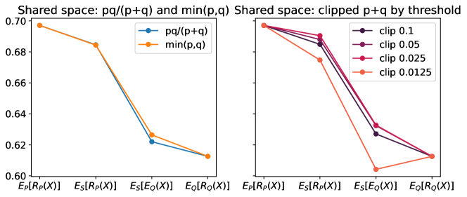
(a) $Y|X$ shift: original model trained on West Virginia and evaluated on Maryland

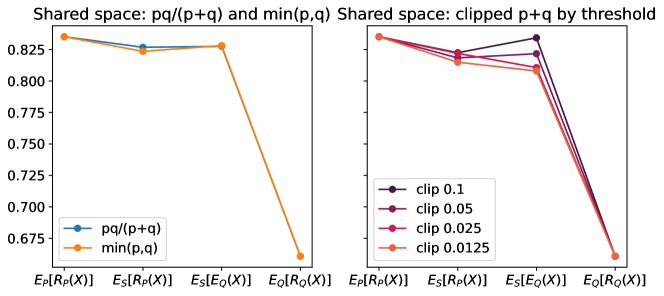
(b) $X$ shift: model trained on only age $\leq$25 and evaluated on general population

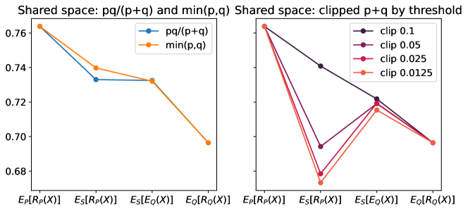
(c) $X$ shift: model trained on over-sampling age $\leq 25$ and evaluated on general population

Figure 7: Comparison of different shared spaces for experiments in Section 4.1. On the $Y$ axis is accuracy; note that all results hold if we replace $\ell(\cdot)$ with accuracy. The leftmost plots correspond to Equations (2.2) and (2.3a), while the rightmost plots correspond to Equation (2.3b). Observe that the decompositions tend to be qualitatively similar across different shared spaces, with the exception of those for Equation (2.3b). Because of the need to choose a threshold for Equation (2.3b) and the sensitivity of decompositions to the threshold value, we do not recommend it. Note that the performance change attributed to $Y\mid X$ does not always correspond to a worsening of performance. In those cases, it could be noise, but it could also be that performance for $Q_{Y\mid X}$ is better than $P_{Y\mid X}$ on the shared $X$ distribution.

References

- Amorim et al. [2018] E. Amorim, M. Cançado, and A. Veloso. Automated essay scoring in the presence of biased ratings. In Association for Computational Linguistics (ACL), pages 229–237, 2018.
- Arjovsky et al. [2019] M. Arjovsky, L. Bottou, I. Gulrajani, and D. Lopez-Paz. Invariant risk minimization. arXiv:1907.02893 [stat.ML], 2019.
- Asmussen and Glynn [2007] S. Asmussen and P. W. Glynn. Stochsatic Simulation: Algorithms and Analysis. Springer, 2007.
- Bandi et al. [2018] P. Bandi, O. Geessink, Q. Manson, M. Van Dijk, M. Balkenhol, M. Hermsen, B. E. Bejnordi, B. Lee, K. Paeng, A. Zhong, et al. From detection of individual metastases to classification of lymph node status at the patient level: the camelyon17 challenge. IEEE transactions on medical imaging, 38(2):550–560, 2018.
- Banerjee et al. [2015] A. Banerjee, D. Karlan, and J. Zinman. Six randomized evaluations of microcredit: Introduction and further steps. American Economic Journal: Applied Economics, 7(1):1–21, 2015.
- Beery et al. [2020] S. Beery, E. Cole, and A. Gjoka. The iwildcam 2020 competition dataset. arXiv:2004.10340 [cs.CV], 2020.
- Ben-David et al. [2007] S. Ben-David, J. Blitzer, K. Crammer, and F. Pereira. Analysis of representations for domain adaptation. In Advances in Neural Information Processing Systems 20, pages 137–144, 2007.
- Ben-Tal et al. [2013] A. Ben-Tal, D. den Hertog, A. D. Waegenaere, B. Melenberg, and G. Rennen. Robust solutions of optimization problems affected by uncertain probabilities. Management Science, 59(2):341–357, 2013.
- Bertsimas et al. [2018] D. Bertsimas, V. Gupta, and N. Kallus. Data-driven robust optimization. Mathematical Programming, Series A, 167(2):235–292, 2018.
- Bickel et al. [1998] P. Bickel, C. A. J. Klaassen, Y. Ritov, and J. Wellner. Efficient and Adaptive Estimation for Semiparametric Models. Springer Verlag, 1998.
- Bickel et al. [2007] S. Bickel, M. Brückner, and T. Scheffer. Discriminative learning for differing training and test distributions. In Proceedings of the 24th International Conference on Machine Learning, 2007.
- Blanchet et al. [2017] J. Blanchet, Y. Kang, F. Zhang, and K. Murthy. Data-driven optimal transport cost selection for distributionally robust optimizatio. arXiv:1705.07152 [stat.ML], 2017.
- Blanchet et al. [2019] J. Blanchet, Y. Kang, and K. Murthy. Robust Wasserstein profile inference and applications to machine learning. Journal of Applied Probability, 56(3):830–857, 2019.
- Buolamwini and Gebru [2018] J. Buolamwini and T. Gebru. Gender shades: Intersectional accuracy disparities in commercial gender classification. In Conference on Fairness, Accountability and Transparency, pages 77–91, 2018.
- Chattopadhyay et al. [2020] A. Chattopadhyay, C. H. Hase, and J. R. Zubizarreta. Balancing vs modeling approaches to weighting in practice. Statistics in Medicine, 39(24), 2020. doi: https://doi.org/10.1002/sim.8659. URL https://onlinelibrary.wiley.com/doi/abs/10.1002/sim.8659.
- Chen et al. [2020] I. Y. Chen, E. Pierson, S. Rose, S. Joshi, K. Ferryman, and M. Ghassemi. Ethical machine learning in health care. arXiv:2009.10576 [cs.SY], 2020.
- Chen et al. [2014] M. S. Chen, P. N. Lara, J. H. Dang, D. A. Paterniti, and K. Kelly. Twenty years post-NIH revitalization act: enhancing minority participation in clinical trials (EMPaCT): laying the groundwork for improving minority clinical trial accrual: renewing the case for enhancing minority participation in cancer clinical trials. Cancer, 120:1091–1096, 2014.
- Chernozhukov et al. [2018] V. Chernozhukov, D. Chetverikov, M. Demirer, E. Duflo, C. Hansen, W. Newey, and J. Robins. Double/debiased machine learning for treatment and structural parameters. The Econometrics Journal, 21(1):C1–C68, 2018.
- Christie et al. [2018] G. Christie, N. Fendley, J. Wilson, and R. Mukherjee. Functional map of the world. In Proceedings of the IEEE Conference on Computer Vision and Pattern Recognition, pages 6172–6180, 2018.
- Chung and Romano [2013] E. Chung and J. P. Romano. Exact and asymptotically robust permutation tests. The Annals of Statistics, 41(2):484 – 507, 2013.
- Colombo et al. [2011] M. Colombo, J. Gondzio, and A. Grothey. A warm-start approach for large-scale stochastic linear programs. Mathematical Programming, 127(2):371–397, 2011.
- Cruces and Galiani [2007] G. Cruces and S. Galiani. Fertility and female labor supply in latin america: New causal evidence. Labour Economics, 14(3):565–573, 2007.
- Crump et al. [2006] R. K. Crump, V. J. Hotz, G. W. Imbens, and O. A. Mitnik. Moving the goalposts: Addressing limited overlap in the estimation of average treatment effects by changing the estimand. Technical report, National Bureau of Economic Research, 2006.
- Dehejia et al. [2021] R. Dehejia, C. Pop-Eleches, and C. Samii. From local to global: External validity in a fertility natural experiment. Journal of Business & Economic Statistics, 39(1):217–243, 2021.
- Delage and Ye [2010] E. Delage and Y. Ye. Distributionally robust optimization under moment uncertainty with application to data-driven problems. Operations Research, 58(3):595–612, 2010.
- Ding et al. [2021] F. Ding, M. Hardt, J. Miller, and L. Schmidt. Retiring adult: New datasets for fair machine learning. Advances in Neural Information Processing Systems 34, 34, 2021.
- Duchi et al. [2022] J. Duchi, T. Hashimoto, and H. Namkoong. Distributionally robust losses for latent covariate mixtures. Operations Research, 2022.
- Duchi and Namkoong [2021] J. C. Duchi and H. Namkoong. Learning models with uniform performance via distributionally robust optimization. Annals of Statistics, 49(3):1378–1406, 2021.
- Efron [1982] B. Efron. The Jackknife, the Bootstrap and Other Resampling Plans. Society for Industrial and Applied Mathematics, 1982. doi: 10.1137/1.9781611970319.
- Egami and Hartman [2022] N. Egami and E. Hartman. Elements of external validity: Framework, design, and analysis. American Political Science Review, page 1–19, 2022.
- Eldar et al. [2004] Y. C. Eldar, A. Ben-Tal, and A. Nemirovski. Linear minimax regret estimation of deterministic parameters with bounded data uncertainties. IEEE Transactions on Signal Processing, 52(8):2177–2188, 2004.
- Elkan [2001] C. Elkan. The foundations of cost-sensitive learning. In International joint conference on artificial intelligence, volume 17, pages 973–978. Lawrence Erlbaum Associates Ltd, 2001.
- Fogarty [2019] C. B. Fogarty. Studentized sensitivity analysis for the sample average treatment effect in paired observational studies. Journal of the American Statistical Association, pages 1–13, 2019.
- Ganin et al. [2016] Y. Ganin, E. Ustinova, H. Ajakan, P. Germain, H. Larochelle, F. Laviolette, M. March, and V. Lempitsky. Domain-adversarial training of neural networks. Journal of Machine Learning Research, 17(59):1–35, 2016.
- Gao et al. [2017] R. Gao, X. Chen, and A. Kleywegt. Wasserstein distributional robustness and regularization in statistical learning. arXiv:1712.06050 [cs.LG], 2017.
- Gertler et al. [2015] P. Gertler, M. Shah, M. L. Alzua, L. Cameron, S. Martinez, and S. Patil. How does health promotion work? evidence from the dirty business of eliminating open defecation. Technical report, National Bureau of Economic Research, 2015.
- Gutman et al. [2022] R. Gutman, E. Karavani, and Y. Shimoni. Propensity score models are better when post-calibrated. arXiv:2211.01221 [stat.ML], 2022. URL https://arxiv.org/abs/2211.01221.
- Hand [2006] D. J. Hand. Classifier technology and the illusion of progress. Statistical Science, 21(1):1–14, 2006.
- Hendrycks et al. [2021] D. Hendrycks, S. Basart, N. Mu, S. Kadavath, F. Wang, E. Dorundo, R. Desai, T. Zhu, S. Parajuli, M. Guo, S. Dawn, J. Steinhardt, and J. Gilmer. The many faces of robustness: A critical analysis of out-of-distribution generalization. In Proceedings of the IEEE/CVF International Conference on Computer Vision, pages 8340–8349, 2021.
- Homma and Saltelli [1996] T. Homma and A. Saltelli. Importance measures in global sensitivity analysis of nonlinear models. Reliability Engineering & System Safety, 52(1):1–17, 1996.
- Huang et al. [2007] J. Huang, A. Gretton, K. M. Borgwardt, B. Schölkopf, and A. J. Smola. Correcting sample selection bias by unlabeled data. In Advances in Neural Information Processing Systems 20, pages 601–608, 2007.
- Huyen [2022] C. Huyen. Designing Machine Learning Systems: An Iterative Process for Production-Ready Applications. O’Reilly, 2022.
- Imai and Ratkovic [2014] K. Imai and M. Ratkovic. Covariate balancing propensity score. Journal of the Royal Statistical Society: Series B (Statistical Methodology), 76(1):243–263, 2014.
- Imbens and Rubin [2015] G. Imbens and D. Rubin. Causal Inference for Statistics, Social, and Biomedical Sciences. Cambridge University Press, 2015.
- Jeong and Namkoong [2020] S. Jeong and H. Namkoong. Assessing external validity over worst-case subpopulations. arXiv:2007.02411 [stat.ML], 2020.
- Kallus and Zhou [2018] N. Kallus and A. Zhou. Confounding-robust policy improvement. In Advances in Neural Information Processing Systems 31, pages 9269–9279, 2018.
- Kallus et al. [2019] N. Kallus, X. Mao, and A. Zhou. Interval estimation of individual-level causal effects under unobserved confounding. In Proceedings of the 22nd International Conference on Artificial Intelligence and Statistics, 2019.
- Kennedy [2022] E. H. Kennedy. Semiparametric doubly robust targeted double machine learning: a review. arXiv:2203.06469 [stat.ME], 2022.
- Kern et al. [2016] H. L. Kern, E. A. Stuart, J. Hill, and D. P. Green. Assessing methods for generalizing experimental impact estimates to target populations. Journal of Research on Educational Effectiveness, 9(1):103–127, 2016.
- Koh et al. [2020] P. W. Koh, S. Sagawa, H. Marklund, S. M. Xie, M. Zhang, A. Balsubramani, W. Hu, M. Yasunaga, R. L. Phillips, S. Beery, et al. Wilds: A benchmark of in-the-wild distribution shifts. arXiv:2012.07421 [cs.LG], 2020.
- Kuhn et al. [2019] D. Kuhn, P. M. Esfahani, V. A. Nguyen, and S. Shafieezadeh-Abadeh. Wasserstein distributionally robust optimization: Theory and applications in machine learning. In Operations Research & Management Science in the Age of Analytics, pages 130–166. INFORMS, 2019.
- Lam [2019] H. Lam. Recovering best statistical guarantees via the empirical divergence-based distributionally robust optimization. Operations Research, 67(4):1090–1105, 2019.
- Lam and Zhou [2015] H. Lam and E. Zhou. Quantifying input uncertainty in stochastic optimization. In Proceedings of the 2015 Winter Simulation Conference. IEEE, 2015.
- Lazaridou et al. [2021] A. Lazaridou, A. Kuncoro, E. Gribovskaya, D. Agrawal, A. Liska, T. Terzi, M. Gimenez, C. de Masson d'Autume, T. Kocisky, S. Ruder, D. Yogatama, K. Cao, S. Young, and P. Blunsom. Mind the gap: Assessing temporal generalization in neural language models. In nips21, 2021.
- Leek et al. [2010] J. T. Leek, R. B. Scharpf, H. C. Bravo, D. Simcha, B. Langmead, W. E. Johnson, D. Geman, K. Baggerly, and R. A. Irizarry. Tackling the widespread and critical impact of batch effects in high-throughput data. Nature Reviews Genetics, 11(10):733–739, 2010.
- Lesko et al. [2017] C. R. Lesko, A. L. Buchanan, D. Westreich, J. K. Edwards, M. G. Hudgens, and S. R. Cole. Generalizing study results: a potential outcomes perspective. Epidemiology (Cambridge, Mass.), 28(4):553, 2017.
- Li et al. [2018] F. Li, K. L. Morgan, and A. M. Zaslavsky. Balancing covariates via propensity score weighting. Journal of the American Statistical Association, 113(521):390–400, 2018.
- Lipton et al. [2018] Z. Lipton, Y.-X. Wang, and A. Smola. Detecting and correcting for label shift with black box predictors. In ICML18, 2018.
- Meinshausen and Bühlmann [2015] N. Meinshausen and P. Bühlmann. Maximin effects in inhomogeneous large-scale data. The Annals of Statistics, 43(4):1801–1830, 2015.
- Miller et al. [2020] J. Miller, K. Krauth, B. Recht, and L. Schmidt. The effect of natural distribution shift on question answering models. In International Conference on Machine Learning, pages 6905–6916. PMLR, 2020.
- Miller et al. [2021] J. Miller, R. Taori, A. Raghunathan, S. Sagawa, P. W. Koh, V. Shankar, P. Liang, Y. Carmon, and L. Schmidt. Accuracy on the line: on the strong correlation between out-of-distribution and in-distribution generalization. In Proceedings of the 38th International Conference on Machine Learning, 2021.
- Miner [1945] M. A. Miner. Cumulative Damage in Fatigue. Journal of Applied Mechanics, 12(3):A159–A164, 1945.
- Miyato et al. [2015] T. Miyato, S.-i. Maeda, M. Koyama, K. Nakae, and S. Ishii. Distributional smoothing with virtual adversarial training. arXiv:1507.00677 [stat.ML], 2015.
- Newey [1994] W. K. Newey. The asymptotic variance of semiparametric estimators. Econometrica, pages 1349–1382, 1994.
- Newey [1997] W. K. Newey. Convergence rates and asymptotic normality for series estimators. Journal of Econometrics, 79(1):147–168, 1997.
- Newey and McFadden [1994] W. K. Newey and D. McFadden. Large sample estimation and hypothesis testing. Handbook of Econometrics, 4:2111–2245, 1994.
- Owen [2014] A. B. Owen. Sobol’ indices and Shapley value. SIAM/ASA Journal on Uncertainty Quantification, 2(1):245–251, 2014.
- Owen [2015] A. B. Owen. Monte Carlo Theory, Methods, and Examples. 2015. Online at http://statweb.stanford.edu/~owen/mc/.
- Paulk et al. [1993] M. Paulk, B. Curtis, M. Chrissis, and C. Weber. Capability maturity model, version 1.1. IEEE Software, 10(4):18–27, 1993.
- Pedregosa et al. [2011] F. Pedregosa, G. Varoquaux, A. Gramfort, V. Michel, B. Thirion, O. Grisel, M. Blondel, P. Prettenhofer, R. Weiss, V. Dubourg, J. Vanderplas, A. Passos, D. Cournapeau, M. Brucher, M. Perrot, and E. Duchesnay. Scikit-learn: Machine learning in Python. Journal of Machine Learning Research, 12:2825–2830, 2011.
- Peters et al. [2016] J. Peters, P. Bühlmann, and N. Meinshausen. Causal inference by using invariant prediction: identification and confidence intervals. Journal of the Royal Statistical Society, Series B, 78(5):947–1012, 2016.
- Praestgaard and Wellner [1993] J. Praestgaard and J. A. Wellner. Exchangeably weighted bootstraps of the general empirical process. The Annals of Probability, 21(4):2053–2086, 1993.
- Pyzdek and Keller [2003] T. Pyzdek and P. A. Keller. Quality engineering handbook. CRC Press, 2003.
- Quiñonero-Candela et al. [2008] J. Quiñonero-Candela, M. Sugiyama, A. Schwaighofer, and N. D. Lawrence. Dataset shift in machine learning. MIT Press, 2008.
- Recht et al. [2019] B. Recht, R. Roelofs, L. Schmidt, and V. Shankar. Do ImageNet classifiers generalize to ImageNet? In Proceedings of the 36th International Conference on Machine Learning, 2019.
- Rosenbaum [2010] P. R. Rosenbaum. Design of Observational Studies. Springer Series in Statistics. Springer, 2010.
- Rosenbaum [2011] P. R. Rosenbaum. A new u-statistic with superior design sensitivity in matched observational studies. Biometrics, 67(3):1017–1027, 2011.
- Rosenfeld et al. [2021] E. Rosenfeld, P. Ravikumar, and A. Risteski. The risks of invariant risk minimization. In Proceedings of the Ninth International Conference on Learning Representations, 2021.
- Rothenhäusler et al. [2018] D. Rothenhäusler, P. Bühlmann, N. Meinshausen, and J. Peters. Anchor regression: heterogeneous data meets causality. arXiv:1801.06229 [stat.ME], 2018.
- Saenko et al. [2010] K. Saenko, B. Kulis, M. Fritz, and T. Darrell. Adapting visual category models to new domains. In Proceedings of the European Conference on Computer Vision, pages 213–226. Springer, 2010.
- Sagawa et al. [2021] S. Sagawa, P. W. Koh, T. Lee, I. Gao, S. M. Xie, K. Shen, A. Kumar, W. Hu, M. Yasunaga, H. Marklund, et al. Extending the wilds benchmark for unsupervised adaptation. In Advances in Neural Information Processing Systems 21, 2021.
- Sahoo et al. [2022] R. Sahoo, L. Lei, and S. Wager. Learning from a biased sample. arXiv:2209.01754 [stat.ME], 2022.
- Saltelli et al. [2008] A. Saltelli, M. Ratto, T. Andres, F. Campolongo, J. Cariboni, D. Gatelli, M. Saisana, and S. Tarantola. Global sensitivity analysis: the primer. John Wiley & Sons, 2008.
- Schölkopf et al. [2012] B. Schölkopf, D. Janzing, J. Peters, E. Sgouritsa, K. Zhang, and J. Mooij. On causal and anticausal learning. In Proceedings of the 29th International Conference on Machine Learning, pages 1255–1262, 2012.
- Shafieezadeh-Abadeh et al. [2015] S. Shafieezadeh-Abadeh, P. M. Esfahani, and D. Kuhn. Distributionally robust logistic regression. In Advances in Neural Information Processing Systems 28, pages 1576–1584, 2015.
- Shankar et al. [2019] V. Shankar, A. Dave, R. Roelofs, D. Ramanan, B. Recht, and L. Schmidt. Do image classifiers generalize across time? arXiv:1906.02168 [cs.LG], 2019.
- Shimodaira [2000] H. Shimodaira. Improving predictive inference under covariate shift by weighting the log-likelihood function. Journal of Statistical Planning and Inference, 90(2):227–244, 2000.
- Song et al. [2016] E. Song, B. L. Nelson, and J. Staum. Shapley effects for global sensitivity analysis: Theory and computation. SIAM/ASA Journal on Uncertainty Quantification, 4(1):1060–1083, 2016.
- Staib and Jegelka [2019] M. Staib and S. Jegelka. Distributionally robust optimization and generalization in kernel methods. In Advances in Neural Information Processing Systems, pages 9131–9141, 2019.
- Stone [1982] C. J. Stone. Optimal global rates of convergence for nonparametric regression. Annals of Statistics, 10(4):1040–1053, 1982.
- Stuart et al. [2011] E. A. Stuart, S. R. Cole, C. P. Bradshaw, and P. J. Leaf. The use of propensity scores to assess the generalizability of results from randomized trials. Journal of the Royal Statistical Society: Series A (Statistics in Society), 174(2):369–386, 2011.
- Sugiyama et al. [2007] M. Sugiyama, M. Krauledat, and K.-R. Müller. Covariate shift adaptation by importance weighted cross validation. Journal of Machine Learning Research, 8:985–1005, 2007.
- Taori et al. [2020] R. Taori, A. Dave, V. Shankar, N. Carlini, B. Recht, and L. Schmidt. Measuring robustness to natural distribution shifts in image classification. In Advances in Neural Information Processing Systems 20, 2020.
- Tipton [2013] E. Tipton. Improving generalizations from experiments using propensity score subclassification: Assumptions, properties, and contexts. Journal of Educational and Behavioral Statistics, 38(3):239–266, 2013.
- Tipton and Olsen [2018] E. Tipton and R. B. Olsen. A review of statistical methods for generalizing from evaluations of educational interventions. Educational Researcher, 47(8):516–524, 2018.
- Tipton and Peck [2017] E. Tipton and L. R. Peck. A design-based approach to improve external validity in welfare policy evaluations. Evaluation review, 41(4):326–356, 2017.
- Tran et al. [2022] D. Tran, J. Liu, M. W. Dusenberry, D. Phan, M. Collier, J. Ren, K. Han, Z. Wang, Z. Mariet, H. Hu, N. Band, T. G. J. Rudner, K. Singhal, Z. Nado, J. van Amersfoort, A. Kirsch, R. Jenatton, N. Thain, H. Yuan, K. Buchanan, K. Murphy, D. Sculley, Y. Gal, Z. Ghahramani, J. Snoek, and B. Lakshminarayanan. Plex: Towards reliability using pretrained large model extensions. arxiv:2207.07411 [stat.ML], 2022.
- Tsuboi et al. [2009] Y. Tsuboi, H. Kashima, S. Hido, S. Bickel, and M. Sugiyama. Direct density ratio estimation for large-scale covariate shift adaptation. Journal of Information Processing, 17:138–155, 2009.
- Tsybakov [2009] A. B. Tsybakov. Introduction to Nonparametric Estimation. Springer, 2009.
- Van Parys et al. [2021] B. P. Van Parys, P. M. Esfahani, and D. Kuhn. From data to decisions: Distributionally robust optimization is optimal. Management Science, 67(6):3387–3402, 2021.
- Wong et al. [2021] A. Wong, E. Otles, J. P. Donnelly, A. Krumm, J. McCullough, O. DeTroyer-Cooley, J. Pestrue, M. Phillips, J. Konye, C. Penoza, et al. External validation of a widely implemented proprietary sepsis prediction model in hospitalized patients. JAMA Internal Medicine, 181(8):1065–1070, 2021.
- Wortsman et al. [2021] M. Wortsman, G. Ilharco, M. Li, J. W. Kim, H. Hajishirzi, A. Farhadi, H. Namkoong, and L. Schmidt. Robust fine-tuning of zero-shot models. arXiv:2109.01903 [cs.CV], 2021.
- Xu et al. [2012] H. Xu, C. Caramanis, and S. Mannor. A distributional interpretation of robust optimization. Mathematics of Operations Research, 37(1):95–110, 2012.
- Yadlowsky [2022] S. Yadlowsky. On cross-fitting with plug-in estimators, Oct 2022. URL https://www.syadlowsky.com/blog/semiparametric/2022/10/24/on-cross-fitting-with-plug-in-estimators.html.
- Yadlowsky et al. [2021] S. Yadlowsky, S. Fleming, N. Shah, E. Brunskill, and S. Wager. Evaluating treatment prioritization rules via rank-weighted average treatment effects. arXiv:2111.07966 [stat.ML], 2021.
- Yadlowsky et al. [2022] S. Yadlowsky, H. Namkoong, S. Basu, J. Duchi, and L. Tian. Bounds on the conditional and average treatment effect with unobserved confounding factors. Annals of Statistics, 50(5):2587–2615, 2022.
- Zech et al. [2018] J. R. Zech, M. A. Badgeley, M. Liu, A. B. Costa, J. J. Titano, and E. K. Oermann. Variable generalization performance of a deep learning model to detect pneumonia in chest radiographs: a cross-sectional study. PLoS medicine, 15(11):e1002683, 2018.
- Zhang et al. [2022] H. Zhang, H. Singh, M. Ghassemi, and S. Joshi. ”why did the model fail?”: Attributing model performance changes to distribution shifts, 2022. URL https://arxiv.org/abs/2210.10769.
- Zhao [2019] Q. Zhao. Covariate balancing propensity score by tailored loss functions. The Annals of Statistics, 47(2):965–993, 2019.
- Zheng and van der Laan [2011] W. Zheng and M. J. van der Laan. Cross-Validated Targeted Minimum-Loss-Based Estimation, pages 459–474. Springer New York, New York, NY, 2011. ISBN 978-1-4419-9782-1. doi: 10.1007/978-1-4419-9782-1˙27. URL https://doi.org/10.1007/978-1-4419-9782-1_27.