The key to understanding complex quantum systems is information scrambling, originally proposed in the Hayden-Preskill recovery. The Hayden-Preskill recovery refers to the phenomena in which localized information is spread over the entire system and becomes accessible from any small subsystem. While this phenomena is well-understood in random unitary models, it has been hardly explored in Hamiltonian systems. In this Letter, we investigate the information recovery for various time-independent Hamiltonians, including chaotic spin chains and Sachdev-Ye-Kitaev (SYK) models. We show that information recovery is possible in certain, but not all, chaotic models, which highlightes that the information recovery differs from other concepts, such as quantum chaos based on energy statistics and the saturation of out-of-time-ordered correlators (OTOCs) for local observables. We further demonstrate that information recovery serves as a powerful tool to probe transitions that originates from the changes of information-theoretic properties of the dynamics.

Hayden-Preskill Recovery in Hamiltonian Systems

A central challenge in modern physics is to characterize the dynamics in far-from-equilibrium quantum systems. The Hayden-Preskill protocol [1] offers an operational approach toward this goal and attracts much attention [2, 3, 4, 5, 6, 7, 8, 9, 10, 11, 12, 13, 14, 15, 16, 17, 18, 19, 20, 21, 22, 23, 24, 10, 25, 26, 27, 28, 29]. The protocol addresses if the information initially localized in a small subsystem can be recovered from other subsystems after unitary time evolution. If the unitary dynamics is sufficiently random, the information rapidly spreads over the system, and information can be recovered from any small subsystem. This phenomenon is known as the Hayden-Preskill recovery.

The discovery of the Hayden-Preskill recovery in sufficiently complex quantum systems substantially accelerated the interdisciplinary research over theoretical physics: it is inspired by the information paradox of black holes [30, 31, 32], is formulated in the language of quantum information, and is investigated by the technique of random matrix theory (RMT) [33, 34]. The unitary dynamics leading to the Hayden-Preskill recovery is referred to as information scrambling [1], and a huge number of studies have been carried out from different perspectives, such as entanglement generation [2, 4], operator mutual information (OMI) [19, 35, 36, 37], and OTOCs [38, 39, 26].

A canonical model of these studies is the SYK model [40, 41, 11, 12] as it is a holographic dual to quantum gravity [14, 13, 42, 43, 44]. The dynamics of SYK model turns out to rapidly saturate OTOCs [11, 12] for local observables and to take the maximum possible value of the quantum Lyapunov exponent [45]. It was also shown to have RMT-like energy statistics, implying that it is quantum chaotic in a conventional notion based on the Bohigas-Giannoni-Schmit (BGS) conjecture [46]. To better understand the model, various variants have been proposed [47], and transitions from quantum chaos to a many-body localization (MBL) have been studied [48, 49].

Despite these progresses, the Hayden-Preskill recovery in time-independent Hamiltonian systems has rarely been explored so far [50]. The Hayden-Preskill recovery is widely believed to be achievable in quantum chaotic systems, but this is yet to be confirmed since the recovery strongly relies on the random unitary assumption that is unlikely to be satisfied even approximately in time-independent Hamiltonian systems [8, 51]. Furthermore, quantum chaos is commonly characterized by eigenenergy statistics which is a static property, but the Hayden-Preskill recovery is about the dynamical properties. Thus, the relation between quantum chaos and the information recovery is not a priori trivial.

In this Letter, we investigate information scrambling in Hamiltonian systems in the sense of the Hayden-Preskill recovery. We first provide a class of Hamiltonians that do not lead to information scrambling. Notably, this includes chaotic spin chains that saturate OTOCs for local observables. We then confirm information scrambling in the Sachdev-Ye-Kitaev (SYK) Hamiltonians and their sparse variants. We further demonstrate that information scrambling captures the transitions in a variant of SYK models, which is not captured by other means, showing that the transition is a manifestation of a drastic change of information-theoretic features of the dynamics.

The Hayden-Preskill protocol.– Given quantum many-body system $S$ of $N$ qubits, we encode quantum information into a localized subsystem $A\subset S$ of $k$ qubits ($k\ll N$). We then let the system $S$ undergo the Hamiltonian time-evolution $U_{\hat{H}}(t):=e^{-i\hat{H}t}$ for some time $t$, where $\hat{H}$ is the Hamiltonian in $S$. After the time-evolution, the information is tried to be recovered from an $\ell$-qubit subsystem $C\subset S$. Throughout our analysis, we assume $C\subset B:=S\setminus A$ as far as $\ell\leq N-k$. The question is how large $\ell$ should be for a successful recovery.

The answer depends on the initial state in $B$ as well as available resources in the recovery process. Here, we assume that the initial state in $B$ is a thermal state $\xi^{B}(\beta)$ at the inverse temperature $\beta$, which is purified to a thermofield-double state $\ket{\xi(\beta)}^{BB^{\prime}}$ by a system $B^{\prime}$. We consider the scenario that the system $B^{\prime}$ can be used in the recovery process. This has a natural interpretation in the black hole information paradox [1]. See Fig. 1.

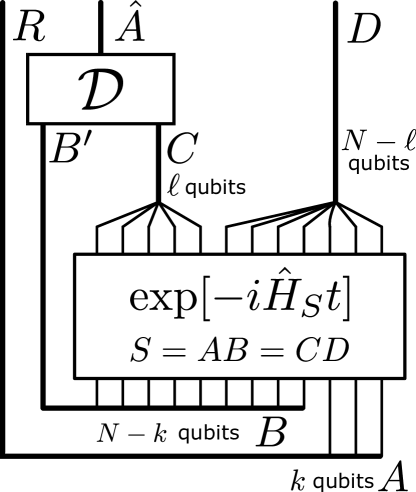
Figure 1: A diagram of the Hayden-Preskill protocol. Time flows from bottom to top. Horizontal lines imply that the qubits connected by the line may be entangled. The initial states on $AR$ and $BB^{\prime}$ are given by a maximally entangled state of $k$ ebits, i.e., $k$ EPR pairs, that keeps track of quantum information in $A$, and a thermofield double state $\ket{\xi(\beta)}$ at the inverse temperature $\beta$ in $B$, respectively. The system $S:=AB$ undergoes Hamiltonian dynamics by $\hat{H}_{S}$, and then, is split into two random subsystems $C$ of $\ell$ qubits and $D$ of $N-\ell$ qubits. By applying a quantum channel ${\mathcal{D}}$ onto $B^{\prime}C$, one aims to decode the quantum information in $A$, that is, to recover the $k$ EPR pairs between $\hat{A}$ and $R$. This protocol has a natural interpretation in the context of information paradox [1]. See also a tutorial [52].

The recovery of quantum information is defined using $k$ Einstein–Podolsky–Rosen (EPR) pairs $\ket{\Phi}^{AR}$ between $A$ and $R$, where the reference system $R$ is virtually introduced for analyses. If we can reproduce $k$ EPR pairs in $AR$ from the state in $B^{\prime}CR$ by a quantum operation $\mathcal{D}$ on $B^{\prime}C$ within some error, then it implies that information in $A$ is recoverable within that error. The precise definition is provided in Supplemental Material S1 [53].

It is in general difficult to compute the recovery error $\Delta_{\hat{H}}(t,\beta)$, which we normalize to be $\Delta_{\hat{H}}\in[0,1]$. Nevertheless, its upper bound can be computed based on the decoupling approach [54, 55, 56]. To this end, we use

$$\Psi_{\rm fin}^{SB^{\prime}R}(t,\beta)=U_{\hat{H}}^{S}(t)(\Phi^{AR}\otimes\xi^{BB^{\prime}})U^{S}_{\hat{H}}(t)^{\dagger}.$$ (1)

Below, we indicate the system over which the partial trace is taken by the superscript, such as $\Psi_{\rm fin}^{DR}(t,\beta)$, where $D=S\setminus C$, is the partial trace of $\Psi_{\rm fin}^{SB^{\prime}R}$ over $CB^{\prime}$. Using this notation, a calculable and typically good upper bound on the recovery error $\Delta_{\hat{H}}(t,\beta)$ is obtained (see Supplemental Material S1 [53])

$$\Delta_{\hat{H}}(t,\beta)\leq\bar{\Delta}_{\hat{H}}(t,\beta):=\min\bigl{\{}1,\sqrt{2\Sigma_{\hat{H}}(t,\beta)}\bigr{\}},$$ (2)

where $\Sigma_{\hat{H}}(t,\beta):=\|\Psi_{\rm fin}^{DR}(t,\beta)-\Psi_{\rm fin}^{D}(t,\beta)\otimes\pi^{R}\|_{1}/2$, $\|\cdot\|_{1}$ is the trace norm, and $\pi^{R}=I^{R}/2^{k}$ is the completely mixed state in $R$.

Note that $\Sigma_{\hat{H}}(t,\beta)$ can be characterized by the mutual information $I(R:D)_{\Psi_{\rm fin}(t,\beta)}=2k-I(R:B^{\prime}C)_{\Psi_{\rm fin}(t,\beta)}$ such that $2\Sigma_{\hat{H}}^{2}/\ln 2\leq I(R:D)_{\Psi_{\rm fin}(t,\beta)}\leq 2k\Sigma_{\hat{H}}+(1+\Sigma_{\hat{H}})h\bigl{(}\Sigma_{\hat{H}}/(1+\Sigma_{\hat{H}})\bigr{)}$, where $h(x)$ is the binary entropy [57]. Since $I(R:D)_{\Psi_{\rm fin}(t,\beta)}$ have been studied in the context of the OMI [19] especially when $\beta=0$, the recovery error can be computed from the OMI (see Supplemental Material S1 [53]), which, however, results in less tight bound. Hence, we focus on $\bar{\Delta}_{\hat{H}}(t,\beta)$.

The recovery error $\Delta_{\hat{H}}(t,\beta)$ is also related to OTOCs: saturation of OTOCs for all observables on $A$ and $C$ implies small recovery error [58, 59]. Hence, by computing OTOCs for all observables, or all the $4^{k+\ell}$ basis operators, on the $k$-qubit subsystem $A$ and the $\ell$-qubit subsystem $C$, one can evaluate the error on recovering $k$-qubit information from an $\ell$-qubit subsystem. While this approach enables us to infer the recovery error from OTOCs, it is computationally intractable since it requires OTOCs for $4^{k+\ell}$ operators. Note that the existing studies of OTOCs in Hamiltonian systems are mostly for the cases with $k=\ell=1$, and hence, do not provide much insight into the recovery error. It is also known that the dynamics of time-independent Hamiltonian is unlikely to saturate OTOCs for all choices of observables [8, 51].

Information scrambling and quantum chaos.– In a random unitary model, the recovery error has been easily computed by using $\Sigma_{\hat{H}}(t,\beta)$ by replacing the time evolution $U^{S}_{\hat{H}}(t)$ with a Haar random unitary. Denoting by $\Delta_{\rm Haar}(\beta)$ the recovery error in this case, it holds with high probability that [1, 56, 24]

$$\Delta_{\rm Haar}(\beta)\leq\bar{\Delta}_{\rm Haar}(\beta):=\min\{1,2^{\frac{1}{2}(\ell_{\rm Haar,th}(\beta)-\ell)}\}.$$ (3)

see Supplemental Material S2 [53]. Note that there is no concept of time $t$ in a random unitary model. Here, $\ell_{\rm Haar,th}(\beta):=\frac{1}{2}\bigl{(}N+k-H(\beta)\bigr{)}$, and $H(\beta)$ is the Renyi-$2$ entropy of $\xi^{B}(\beta)$, defined by $2^{-H(\beta)}=\Tr[\bigl{(}\xi^{B}(\beta)\bigl{)}^{2}\bigr{]}$.

It is clear from Eq. (3) that $\Delta_{\rm Haar}(\beta)\ll 1$ if $\ell\gg\ell_{\rm Haar,th}(\beta)$. In particular, $\ell_{\rm Haar,th}(0)=k$. Hence, if the system is initially at infinite temperature, the $k$-qubit quantum information in $A$ is recoverable from any subsystem of the size that is independent of $N$. This is the Hayden-Preskill recovery. Following the original proposal [1], we refer to the dynamics achieving the Hayden-Preskill recovery as information scrambling. Although information scrambling is commonly rephrased as quantum chaos, we clearly distinguish them: quantum chaos is based on a RMT-like eigenenergy spectrum.

Hamiltonians without information scrambling.– We start with a class of Hamiltonians that turn out not to be information scrambling. We first show that any commuting Hamiltonians, where each Hamiltonian term commutes with each other, fail to be information scrambling due to a lack of information spreading (see Supplemental Material S3 [53]). This may be of interest since certain commuting Hamiltonians show chaotic features [60, 61].

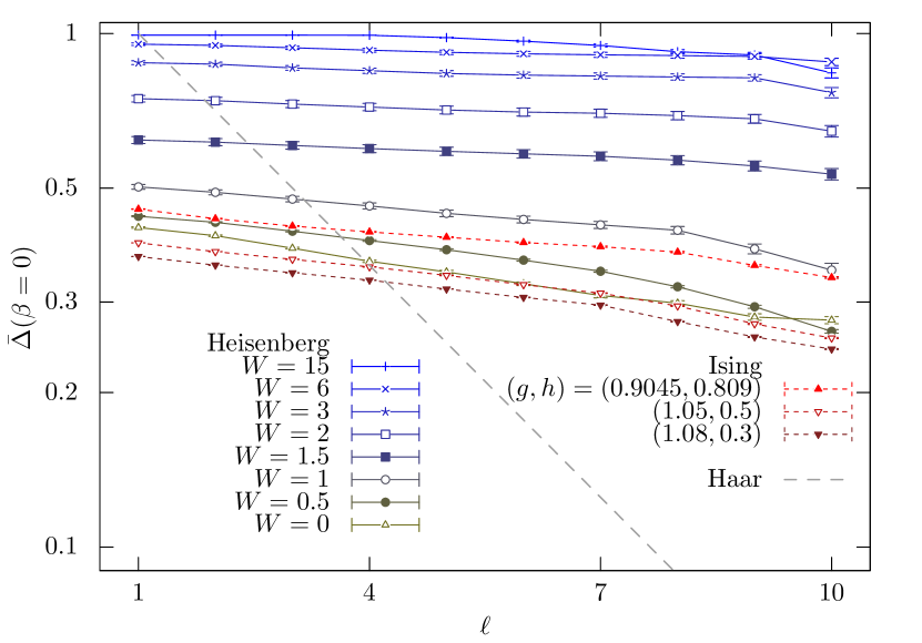
Figure 2: Semilogarithmic plot of the late-time value of $\bar{\Delta}$ for $N=12$, $\beta=0$ for the Heisenberg spin chain with a site-random magnetic field $h_{z}^{j}\in[-W,W]$ parallel to the $z$ direction and for the Ising spin chain with a uniform magnetic field $g\hat{\mathbf{x}}+h\hat{\mathbf{z}}$. The values of $(g,h)$ are those discussed in [62]. The average for $t=(1,2,.\ldots,10)\times 10^{6}$ is plotted as the late-time value. 16 samples are taken for random-field average.

Other Hamiltonians that are not information scrambling are the spin-$1/2$ chains such as the Heisenberg with random magnetic field, $\hat{H}_{\mathrm{XXZ}}=\sum_{j=1}^{N-1}\left(S_{j}^{x}S_{j+1}^{x}+S_{j}^{y}S_{j+1}^{y}+J_{z}S_{j}^{z}S_{j+1}^{z}\right)+\sum_{j=1}^{N}h_{j}S_{j}^{z}$, where $h_{j}$ are independently sampled from a uniform distribution in $[-W,W]$, and the mixed-field Ising with constant magnetic field, $\hat{H}_{\mathrm{Ising}}=-\sum_{j=1}^{N-1}\left(S_{j}^{z}S_{j+1}^{z}\right)-g\sum_{j=1}^{N}S_{j}^{x}-h\sum_{j=1}^{N}S_{j}^{z}$. Both Hamiltonians show integrable–chaotic transitions by varying the magnetic fields [63, 64, 65, 66, 67, 68, 69, 70, 71, 72, 73, 74, 75, 76, 77, 78, 79, 80, 81, 82, 83, 62]. However, our numerical analysis reveals that the recovery errors remain high values for any value of the magnetic fields at any time $t$ (see Supplemental Materials S4 and S5 [53]). See Fig. 2 for the late-time value of $\bar{\Delta}_{\hat{H}}$ for those Hamiltonians at infinite temperature. Note that the absence of information scrambling for these Hamiltonians does not contradict to the saturation of OTOCs for local, typically single-qubit, observables at late time for certain strength of magnetic fields [84, 85, 86, 87, 88, 89]. It is rather likely that OTOCs for multi-qubit oservables are not saturated in such systems [58, 59], which shall be inherent in time-independent Hamiltonian systems [8, 51].

From these chaotic spin chains, it is clear that neither quantum chaotic features in the sense of energy spectrum nor the saturation of OTOCs for local observables implies the Hayden-Preskill recovery. This leads to the necessity of the direct analysis of the information recovery in Hamiltonian systems.

Original and sparse SYK Hamiltonians.– We next investigate the SYK model, $\mathrm{SYK}_{4}$, consisting of $2{N_{\mathrm{q}}}$ Majorana fermions. The Hamiltonian is

$$\hat{H}_{\mathrm{SYK}_{4}}=\sum_{1\leq a_{1}<a_{2}<a_{3}<a_{4}\leq 2{N_{\mathrm{q}}}}J_{a_{1}a_{2}a_{3}a_{4}}\hat{\psi}_{a_{1}}\hat{\psi}_{a_{2}}\hat{\psi}_{a_{3}}\hat{\psi}_{a_{4}},$$ (4)

with $\hat{\psi}_{j}$ being Majorana fermion operators. The couplings $J_{a_{1}a_{2}a_{3}a_{4}}$ are independently chosen at random from the Gaussian with average zero and $\sigma^{2}=\binom{2{N_{\mathrm{q}}}}{4}^{-1}$. Since the parity symmetry of $\mathrm{SYK}_{4}$ leads to deviations in the information recovery [10, 9, 24, 90], we focus on the even-parity sector and set $N={N_{\mathrm{q}}}-1$. A Haar random unitary in the corresponding situation provides the recovery error $\bar{\Delta}^{\prime}_{\rm Haar}(\beta)=\min\{1,2^{(\ell_{\rm Haar,th}(\beta)-\ell)-\frac{1}{4}}\}$. See Supplemental Material S6 [53] for details. We have also checked that the effect by the periodicity, characterized by ${N_{\mathrm{q}}}\mod 4$, is negligible.

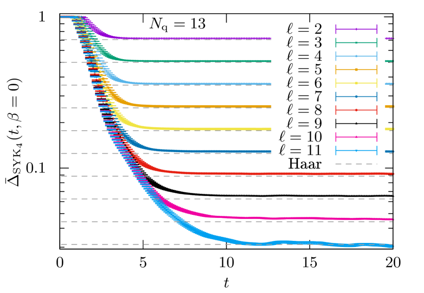
Figure 3: Semilogarithmic plot of the value of $\bar{\Delta}_{\hat{H}_{\mathrm{SYK}_{4}}}(t,\beta=0)$ against $t$ for $k=1,{N_{\mathrm{q}}}=13$, and $2\leq\ell<{N_{\mathrm{q}}}-k$. Average over 64 samples is taken. For $\ell=1$, $\bar{\Delta}_{\hat{H}_{\mathrm{SYK}_{4}}}(t,\beta=0)$ is $\sim 1$ for all $t$. The dashed lines represent $\bar{\Delta}^{\prime}_{\rm Haar}(\beta=0)=2^{\frac{1}{2}(1-\ell)}$ given in Eq. (3) for $\ell=2,3,\ldots,{N_{\mathrm{q}}}-2$. For smaller values of ${N_{\mathrm{q}}}$ and finite $\beta$, see respectively Fig. S5 and Fig. S6 in the Supplemental Material S6 [53].

In Fig. 3, we numerically plot the upper bound on the recovery error, $\bar{\Delta}_{\mathrm{SYK}_{4}}(t,\beta=0)$, against time $t$ for various $\ell$. It clearly shows that $\bar{\Delta}_{\mathrm{SYK}_{4}}$ quickly approaches $\bar{\Delta}^{\prime}_{\rm Haar}$. This is also the case for $\beta>0$. We estimate that $\bar{\Delta}_{\mathrm{SYK}_{4}}$ converges to $\bar{\Delta}^{\prime}_{\rm Haar}$ within time $O(\sqrt{{N_{\mathrm{q}}}})$, which qualitatively supports the fast scrambling conjecture [2, 3, 4]. Hence, the $\mathrm{SYK}_{4}$ dynamics, while differs from Haar random, has an excellent agreement with the prediction by RMT and achieves the Hayden-Preskill recovery.

The situation remains the same even even for a sparse simplification $\mathrm{spSYK}_{4}$ of $\mathrm{SYK}_{4}$. In $\mathrm{spSYK}_{4}$, the number of non-zero random coupling constant is fixed to ${K_{\mathrm{cpl}}}$. It recovers $\mathrm{SYK}_{4}$ when ${K_{\mathrm{cpl}}}=\binom{2{N_{\mathrm{q}}}}{4}$, but ${K_{\mathrm{cpl}}}=O({N_{\mathrm{q}}})$ is known to suffice to have chaotic features and to reproduce holographic properties [91, 92].

In Fig. 4, we plot the upper bound on the recovery error for a further simplified sparse SYK model ($\pm\mathrm{spSYK}_{4}$), in which a half of the non-zero couplings is set to $1/\sqrt{{K_{\mathrm{cpl}}}}$ and the other half to $-1/\sqrt{{K_{\mathrm{cpl}}}}$ [93]. We clearly observe that the value is nearly identical to the Haar value for ${K_{\mathrm{cpl}}}\gtrsim 30$, which is of order ${N_{\mathrm{q}}}$. This implies that $\pm\mathrm{spSYK}_{4}$ with ${K_{\mathrm{cpl}}}=O({N_{\mathrm{q}}})$, which is substantially smaller than ${K_{\mathrm{cpl}}}=O({N_{\mathrm{q}}}^{4})$ of $\mathrm{SYK}_{4}$, suffices also to reproduce information-theoretic properties of $\mathrm{SYK}_{4}$. See Supplemental Material S7 [53] for details. This would help experimental realizations of the model.

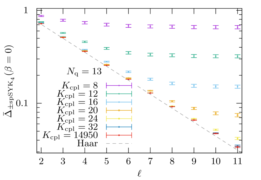
Figure 4: The late-time value of $\bar{\Delta}_{\pm\mathrm{spSYK}_{4}}(t,\beta=0)$ against $\ell$ is plotted for $k=1$ and various numbers ${K_{\mathrm{cpl}}}$ of non-zero coupling constant. We set ${N_{\mathrm{q}}}$ to $13$, and the number of samples is 64. The average for $t=(1,2,\ldots,10)\times 10^{6}$ is plotted as the late-time value in all figures.

Probing transitions by the Hayden-Preskill protocol.– Yet another SYK model attracting much attention is the $\mathrm{SYK}_{4+2}$ model [94]. The Hamiltonian is

$$\hat{H}_{\mathrm{SYK}_{4+2}}(\theta)=\cos\theta\,\hat{H}_{\mathrm{SYK}_{4}}+\sin\theta\,\hat{H}_{\mathrm{SYK}_{2}},$$ (5)

where $\hat{H}_{\mathrm{SYK}_{2}}=i\sum_{1\leq b_{1}<b_{2}\leq 2{N_{\mathrm{q}}}}K_{b_{1}b_{2}}\hat{\psi}_{b_{1}}\hat{\psi}_{b_{2}}$, and $\theta\in[0,\pi/2]$ is a mixing parameter. The coupling constants $\{K_{b_{1}b_{2}}\}$ satisfy $K_{b_{2}b_{1}}=-K_{b_{1}b_{2}}$ and are normalized for the variance of eigenenergies of $\hat{H}_{\mathrm{SYK}_{4+2}}(\theta)$ to be unity.

The $\mathrm{SYK}_{4+2}$ model has a peculiar energy-shell structure in the sense of the local density of states in Fock space, which is drastically changed by varying $\theta$. Accordingly, the range of $\theta\in[0,\pi/2]$ is divided into four regimes I, II, III, and IV [48, 49]. In I, only one energy-shell is dominant in the whole Hilbert space, and it is quantum chaotic. As $\theta$ increases the size of the energy-shell becomes diminished, and ${\mathcal{O}}({\rm poly}({N_{\mathrm{q}}}))$ energy-shells appear in II and III. The energy statistics remains RMT-like in these two regimes. Characterizing physics in II and III has been under intense investigations [95]. In IV, the number of energy-shell approaches ${\mathcal{O}}(\exp({N_{\mathrm{q}}}))$, and Fock-space localization is observed.

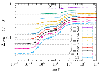
Figure 5: The late-time value of $\bar{\Delta}_{\mathrm{SYK}_{4+2}}(t,\beta=0)$ plotted for $k=1$ and various $\ell$ against the value of $\delta$. ${N_{\mathrm{q}}}$ is set to $13$. 64 samples are used. The lines connecting the data points are guide to the eye. The horizontal dashed lines indicate $\bar{\Delta}^{\prime}_{\rm Haar}$ for various $\ell$.

From the Hayden-Preskill protocol in $\mathrm{SYK}_{4+2}$, each regime can be operationally characterized. In Fig. 5, we plot the late time values of the upper bound $\bar{\Delta}_{\mathrm{SYK}_{4+2}}(t,\beta=0)$ of the recovery error against $\tan\theta$. Two characteristic values of $\theta$, $\tan\theta_{1}\approx 0.5$ and $\tan\theta_{2}\approx 20$, are observed, by which three plateaus appear. In the first plateau ($\theta\in[0,\theta_{1})$) corresponding to the regime I, $\bar{\Delta}_{\mathrm{SYK}_{4+2}}\approx\bar{\Delta}^{\prime}_{\rm Haar}$ and the system is information scrambling. The second is for $\theta\in(\theta_{1},\theta_{2}]$, corresponding to II and III, where $\bar{\Delta}_{\mathrm{SYK}_{4+2}}$ is substantially larger than $\bar{\Delta}^{\prime}_{{\rm Haar}}$. The difference between them seems to remain constant even if ${N_{\mathrm{q}}}$ increases (see Supplemental Material S8 [53]). The third plateau, $\theta\in(\theta_{2},\pi/2]$, corresponds to IV, where the system is almost $\mathrm{SYK}_{2}$.

For sufficiently small and large $\theta$, the behaviour of $\bar{\Delta}_{\mathrm{SYK}_{4+2}}$ can be naturally understood. For small $\theta$, the model is approximately $\mathrm{SYK}_{4}$. Since the dynamics of $\mathrm{SYK}_{4}$ quickly achieves the Hayden-Preskill recovery, so does that in the regime I. In contrast, for sufficiently large $\theta$, the model is almost $\mathrm{SYK}_{2}$ and the Fock-space localization occurs. Hence, the recovery error should remain a large constant in the regime IV due to a lack of information spreading. In contrast, $\bar{\Delta}_{\mathrm{SYK}_{4+2}}$ is smoothly changing for the intermediate values of $\theta$, which is seemiongly in tension with the division of the regimes II and III in terms of the energy-shell structure.

To understand the intermediate plateau, we shall recall that, in II and III, transitions from one energy-shell to the other are strongly suppressed, which effectively results in the division of the whole Hilbert space into ${\mathcal{O}}({\rm poly}({N_{\mathrm{q}}}))$ energy-shells [48]. Additionally, it is known that the dynamics in each energy-shell seems to be approximately Haar random within the subspace [49]. The intermediate plateau of $\bar{\Delta}_{\mathrm{SYK}_{4+2}}$ can be explained from these common features in II and III. Since the whole Hilbert space is effectively divided into smaller ones, within which the dynamics remains still Haar random, the unitary dynamics in II and III induces partial decoupling [96] rather than decoupling. While decoupling results in the Hayden-Preskill recovery (Eq. (3)), partial decoupling leads to the recovery error into the form of $2^{\ell^{\prime}_{\rm th}-\ell}+\Delta_{\rm rem}$ [24]. Here, $\ell^{\prime}_{\rm th}\approx\ell_{\rm Haar,th}+O(\sqrt{k})$ and $\Delta_{\rm rem}$, which is inverse proportional to the standard deviation of energy in the subsystem $D$, represents the amount of information that cannot be recovered even when $\ell$ is large. While $\ell^{\prime}_{\rm th}$ is hardly observed in our analysis, as we set $k=1$, we can clearly observe $\Delta_{\rm rem}$ as an intermediate plateau. Since the standard deviation of energy in $B$ shall be $O(\sqrt{{N_{\mathrm{q}}}})$, that in the subsystem $D$ is at least $O(\sqrt{{N_{\mathrm{q}}}})$. This provides a qualitative estimation, $\Delta_{\rm rem}=O(1/\sqrt{{N_{\mathrm{q}}}})$, of the recovery error in the plateau even for large $\ell$.

From this perspective, the two transitions can be understood as consequences of drastic changes of the decoupling properties induced by the dynamics. In I, the combined regime over II and III, and IV, the $\mathrm{SYK}_{4+2}$ dynamics leads to full, partial, and no decoupling, respectively. Accordingly, each regime has qualitatively different information-theoretic properties and results in different behaviours of information recovery. The emerging difference between II and III should be an artifact due to the fact that the energy shell is viewed in the Fock basis. Since the choice of basis is not intrinsic, the difference between II and III is not observed in terms of the information recovery.

It is worth noting that the information recovery provides an operational probe for characterizing $\mathrm{SYK}_{4+2}$ in the experimentally-realizable manner. This is in contrast to the eigenenergy and eigenstates statistics, which are in general difficult to experimentally access.

Summary and discussions.– In this Letter, we have studied information scrambling in the sense of the Hayden-Preskill recovery and have shown that neither quantum chaotic energy statistics nor the saturation of OTOCs for local observables implies the Hayden-Preskill recovery. We have also shown that the Hayden-Preskill protocol serves as a powerful and operational tool that can information-theoretically characterize the transitions in $\mathrm{SYK}_{4+2}$, which cannot be captured by conventional concepts. It will be of interest to further explore this direction of characterizing various quantum phases in the information-theoretic manner, which may help our understanding of complex quantum many-body dynamics.

The work was supported by Grants-in-Aid for Transformative Research Areas (A) No. JP21H05182, No. JP21H05183 and No. JP21H05185 from MEXT of Japan. The work of M.T. was partly supported by Grants-in-Aid No. JP20H05270 and No. JP20K03787 from MEXT of Japan. Y.N. was supported by JST, PRESTO Grant Number JPMJPR1865, Japan, and by JSPS KAKENHI Grant Number JP22K03464, Japan. Part of the computation in this paper was conducted using the Supercomputing Facilities of the Institute for Solid State Physics, University of Tokyo. The authors thank Satyam S. Jha for collaboration in the early stage of the work. M.T. also thanks Masanori Hanada, Chisa Hotta, and Norihiro Iizuka for valuable discussions.

Supplemental Materials: Hayden-Preskill Recovery in Hamiltonian Systems

S1 Upper and lower bounds on the recovery error

In this section, we derive an upper bound on the recovery error in the Hayden-Preskill protocol based on the decoupling approach [54, 55, 56]. The recovery error in a Hamiltonian system is defined by

$$\Delta_{\hat{H}}(t,\beta):=\frac{1}{2}\min_{{\mathcal{D}}}\norm{\Phi^{AR}-{\mathcal{D}}^{CB^{\prime}\rightarrow A}\bigl{(}\Psi_{\rm fin}^{CB^{\prime}R}(t)\bigr{)}}_{1},$$ (S1)

where the minimum is taken over all CPTP maps ${\mathcal{D}}$ from $CB^{\prime}$ to $A$, $\Psi_{\rm fin}^{CB^{\prime}R}(t,\beta)=\Tr_{D}[\Psi_{\rm fin}^{SB^{\prime}R}(t,\beta)]$, and

$$\ket{\Psi_{\rm fin}(t,\beta)}^{SB^{\prime}R}=e^{-i\hat{H}_{S}t}\bigl{(}\ket{\Phi}^{AR}\otimes\ket{\xi(\beta)}^{BB^{\prime}}\bigr{)}.$$ (S2)

Here, $\hat{H}_{S}$ being the Hamiltonian in the system $S=AB=CD$ of $N$ qubits. $\xi^{BB^{\prime}}(\beta)$ is a thermofield-double state in $BB^{\prime}$ of a thermal state $\xi(\beta)^{B}$ at the inverse temperature $\beta$.

Below, we show

$$1-\sqrt{1-\bigl{(}\Sigma^{\rm opt}_{\hat{H}}(t,\beta)\bigr{)}^{2}}\leq\Delta_{\hat{H}}(t,\beta)\leq\min\bigl{\{}1,\sqrt{2\Sigma^{\rm opt}_{\hat{H}}(t,\beta)}\bigr{\}}.$$ (S3)

Here, $\Sigma^{\rm opt}_{\hat{H}}(t,\beta)$ is the degree of decoupling between $D$ and $R$, defined by

$$\Sigma^{\rm opt}_{\hat{H}}(t,\beta):=\frac{1}{2}\min_{\sigma}\norm{\Psi_{\rm fin}^{DR}(t,\beta)-\sigma^{D}\otimes\pi^{R}}_{1},$$ (S4)

where the minimization is taken over all quantum states on $D$, and $\Psi_{\rm fin}^{DR}(t,\beta)=\Tr_{C}[\Psi_{\rm fin}^{CB^{\prime}R}(t,\beta)]$. This implies that $\Sigma^{\rm opt}_{\hat{H}}(t,\beta)\ll 1$ is essentially necessary and sufficient for the recovery error to be small. This is a well-known relation, but we show it for the sake of completeness. In the derivation, we do not explicitly write $(t,\beta)$.

We use the trace distance between $\rho$ and $\sigma$ by $T(\rho,\sigma)$, i.e.,

$$T(\rho,\sigma):=\frac{1}{2}\norm{\rho-\sigma}_{1}.$$ (S5)

For pure states $\ket{\phi}$ and $\ket{\psi}$, we denote the trace distance by $T(\ket{\phi},\ket{\psi})=\frac{1}{2}\norm{\outerproduct{\phi}{\phi}-\outerproduct{\psi}{\psi}}_{1}$ for simplicity. To obtain the lower bound, we use the relation between the trace distance and the fidelity:

$$1-\sqrt{F(\rho,\sigma)}\leq T(\rho,\sigma)\leq\sqrt{1-F(\rho,\sigma)},$$ (S6)

where $F(\rho,\sigma):=\|\sqrt{\rho}\sqrt{\sigma}\|_{1}^{2}$ is the fidelity. We also use the Uhlmann’s theorem:

$$F(\rho^{A},\sigma^{A})=\max_{V}\bigl{|}\bra{\rho}^{AB}V^{C\rightarrow B}\ket{\sigma}^{AC}\bigr{|}^{2},$$ (S7)

where the maximization is over all isometries $V^{C\rightarrow B}$ from $C$ to $B$ ($\dim\mathcal{H}_{C}\leq\dim\mathcal{H}^{B}$), and $\ket{\rho}^{AB}$ and $\ket{\sigma}^{AC}$ are purifications of $\rho^{A}$ and $\sigma^{A}$, respectively.

The upper bound directly follows from the Uhlmann’s theorem in terms of the trace norm (see, e.g., [56]). It states that, if there are two states $\rho^{A}$ and $\sigma^{A}$ such that $T(\rho,\sigma)\leq\epsilon$, then there exists systems $B$ ($C$) that purifies $\rho^{A}$ ($\sigma^{A}$) to a pure state $\ket{\rho}^{AB}$ ($\ket{\sigma}^{AC})$ and a partial isometry $V^{B\rightarrow C}$ that satisfies $T(V^{B\rightarrow C}\ket{\rho}^{AB},\ket{\sigma}^{AC})\leq\sqrt{2\epsilon}$.

Recall that a purification of $\Psi_{\rm fin}^{DR}(t,\beta)$ is $\ket{\Psi_{\rm fin}(t,\beta)}^{SB^{\prime}R}$ and that that of $\pi^{R}$ is $\ket{\Phi}^{\hat{A}R}$. Hence, denoting by $\ket{\sigma}^{DE}$ a purification of $\sigma^{D}$ in Eq. (S4) by some system $E$, there is a partial isometry $V^{DB^{\prime}\rightarrow\hat{A}E}$ such that

$$T\bigl{(}V^{DB^{\prime}\rightarrow\hat{A}E}\ket{\Psi_{\rm fin}(t,\beta)}^{SB^{\prime}R},\ket{\sigma}^{DE}\otimes\ket{\Phi}^{\hat{A}R}\bigr{)}\leq\sqrt{2\Sigma^{\rm opt}_{\hat{H}}}.$$ (S8)

By tracing out $DE$, we obtain

$$T\bigl{(}{\mathcal{D}}^{DB^{\prime}\rightarrow\hat{A}}\ket{\Psi_{\rm fin}(t,\beta)}^{CB^{\prime}R},\ket{\Phi}^{\hat{A}R}\bigr{)}\leq\sqrt{2\Sigma^{\rm opt}_{\hat{H}}},$$ (S9)

where ${\mathcal{D}}$ is a CPTP map obtained from the isometry $V$ and the partial trace. As the left-hand side is exactly $\Delta_{\hat{H}}$, this provides an upper bound of the recovery error.

The lower bound in Eq. (S3) is obtained using Eqs. (S6) and (S7):

$$\Delta_{\hat{H}} :=\min_{{\mathcal{D}}}T\bigl{(}\Phi^{AR},{\mathcal{D}}^{CB^{\prime}\rightarrow A}\bigl{(}\Psi_{\rm fin}^{CB^{\prime}R}\bigr{)}\bigr{)}$$ (S10)

$$\geq\min_{{\mathcal{D}}}\bigl{\{}1-\sqrt{F\bigl{(}\Phi^{AR},{\mathcal{D}}^{CB^{\prime}\rightarrow A}(\Psi_{\rm fin}^{CB^{\prime}R})}\bigr{)}\bigr{\}}$$ (S11)

$$=\min_{V,\sigma}\bigl{\{}1-|\bra{\Psi_{\rm fin}}^{SB^{\prime}R}V^{AS^{\prime}\rightarrow B^{\prime}C}(\ket{\Phi}^{AR}\otimes\ket{\sigma}^{DS^{\prime}})|\bigr{\}}$$ (S12)

$$\geq\min_{\sigma}\bigl{\{}1-\sqrt{F(\Psi_{\rm fin}^{DR},\pi^{R}\otimes\sigma^{D})}\bigr{\}}$$ (S13)

$$\geq\min_{\sigma}\bigl{\{}1-\sqrt{1-\bigl{(}T(\Psi_{\rm fin}^{DR},\pi^{R}\otimes\sigma^{D})\bigr{)}^{2}}\bigr{\}}$$ (S14)

$$\geq 1-\sqrt{1-\bigl{(}\Sigma^{\rm opt}_{\hat{H}}\bigr{)}^{2}}.$$ (S15)

Here, the second and the second last lines follow from Eq. (S6), the third line from the Uhlmann’s theorem, and the fourth line from the monotonicity of the fidelity under the partial trace.

The degree of decoupling $\Sigma^{\rm opt}_{\hat{H}}$ is still computationally intractable in general due to the minimization over all states in $D$. However, it typically suffices to set the state $\sigma$ in Eq. (S4) to $\Psi_{\rm fin}^{D}$. Thus, we define

$$\Sigma_{\hat{H}}(t,\beta):=\frac{1}{2}\norm{\Psi_{\rm fin}^{DR}(t,\beta)-\Psi_{\rm fin}^{D}(t,\beta)\otimes\pi^{R}}_{1},$$ (S16)

and investigate $\Sigma_{\hat{H}}(t,\beta)$ in our analysis. The corresponding upper bound is

$$\Delta_{\hat{H}}(t,\beta)\leq\bar{\Delta}_{\hat{H}}(t,\beta):=\min\bigl{\{}1,\sqrt{2\Sigma_{\hat{H}}(t,\beta)}\bigr{\}}.$$ (S17)

The degree of decoupling $\Sigma_{\hat{H}}(t,\beta)$ can be characterized by the mutual information between $D$ and $R$. To this end, we start with

$$\frac{2}{\ln 2}\delta^{2}\leq I(X:Y)_{\varrho}\leq 2\delta\log[\min\{d_{X},d_{Y}\}\bigr{]}+(1+\delta)h\biggl{(}\frac{\delta}{1+\delta}\biggr{)},$$ (S18)

where $\delta=\frac{1}{2}\|\varrho^{XY}-\varrho^{X}\otimes\varrho^{Y}\|_{1}$, $d_{W}$ is the dimension of the Hilbert space of $W$ ($W=X,Y$), and $h(x)=-x\log x-(1-x)\log(1-x)$ is the binary entropy. See, e.g., [57]. Setting $X=D$ and $Y=R$, we have

$$\frac{2}{\ln 2}\Sigma_{\hat{H}}^{2}\leq I(R:D)_{\Psi_{\rm fin}(t,\beta)}\leq 2k\Sigma_{\hat{H}}+(1+\Sigma_{\hat{H}})h\biggl{(}\frac{\Sigma_{\hat{H}}}{1+\Sigma_{\hat{H}}}\biggr{)},$$ (S19)

when $k\leq N-\ell$. This might be of independent importance since $I(D:R)_{\Psi_{\rm fin}}$ has been studied as the OMI, especially for the infinite temperature ($\beta=0$) [19, 35, 36, 37]. Hence, it shall be possible to quantitatively connect a number of results on the OMI with the recovery error in the Hayden-Preskill protocol. Note that, in relation to the Hayden-Preskill protocol, $R$ is the system carrying quantum information and $D$ corresponds to the subsystem that is traced out, which corresponds to the remaining black hole in the context of the information paradox. Hence, the size of the subsystems $D$ and $R$ should be $k$ and $N-\ell$. This implies that the parameters of the OMI relevant to the Hayden-Preskill recovery is $k=|R|\ll|D|=N-\ell$, whereas it is sometimes set to $|R|\approx|D|$ in the study of the OMI.

From Eq. (S19), we also have

$$\Sigma_{\hat{H}}(t,\beta)^{2} \leq\frac{\ln 2}{2}I(D:R)_{\Psi_{\rm fin}}$$ (S20)

$$=\frac{\ln 2}{2}\bigl{(}S(D)_{\Psi_{\rm fin}}+S(R)_{\Psi_{\rm fin}}-S(DR)_{\Psi_{\rm fin}}\bigr{)}$$ (S21)

$$=\frac{\ln 2}{2}\bigl{(}S(D)_{\Psi_{\rm fin}}+k-S(CB^{\prime})_{\Psi_{\rm fin}}\bigr{)},$$ (S22)

where we used in the last line the fact that $\Psi_{\rm fin}^{SC^{\prime}R}$ is a pure state. Hence, we have another upper bound on the recovery error in terms of the entropies:

$$\Delta_{\hat{H}}(t,\beta)\leq\min\biggl{\{}1,\biggl{(}2\ln 2\bigl{(}S(D)_{\Psi_{\rm fin}}+k-S(CB^{\prime})_{\Psi_{\rm fin}}\bigr{)}\biggr{)}^{1/4}\biggr{\}}.$$ (S23)

S2 Hayden-Preskill recovery by a Haar random dynamics

To compute the recovery error when the unitary is given by a Haar random unitary, we consider the degree of decoupling $\Sigma_{\rm Haar}(\beta)$ defined by

$$\Sigma_{\rm Haar}(\beta):=\frac{1}{2}\|\Psi_{\rm fin}^{DR}(t,\beta)-\Psi_{\rm fin}^{D}(t,\beta)\otimes\pi^{R}\|_{1},$$ (S24)

where the unitary is Haar random. It is well known that this can be easily computed on average. The result in general cases is summarized to the so-called one-shot decoupling theorem [55], which in our case reads

$$\log[2\mathbb{E}_{U}[\Sigma_{\rm Haar}(\beta)]\bigr{]}\leq-\frac{1}{2}\biggl{(}H_{2}(S|R)_{\xi\otimes\Phi}+H_{2}(\tilde{S}|D)_{\tau}\biggr{)},$$ (S25)

where $\mathbb{E}_{U}$ is the average over a Haar random unitary, and $H_{2}(X|Y)_{\rho}$ is the conditional collision entropy for the state $\rho$. Here and in the following, $\log$ denotes logarithm to base $2$ unless stated otherwise. The state $\tau^{\tilde{S}D}$ is defined by introducing a virtual system $\tilde{S}$ that has the same structure of $S$. That is, $\tilde{S}$ consists of $N$ qubits and can be decomposed as $\tilde{C}\tilde{D}$. The state is given by

$$\tau^{S\tilde{D}}=\Tr_{\tilde{C}}\bigl{[}\outerproduct{\Phi}{\Phi}^{S\tilde{S}}\bigr{]}=\frac{I^{C}}{2^{\ell}}\otimes\outerproduct{\Phi}{\Phi}^{D\tilde{D}},$$ (S26)

where $\Phi^{S\tilde{S}}$ is the maximally entangled state between $S$ and $\tilde{S}$. The conditional collision entropy differs from the conditional von Neumann entropy in general, but when $\beta=0,\infty$, they take the same values. Below, we denote it simply by $H(X|Y)_{\rho}$.

It is also known that a Haar random unitary shows the concentration of measure phenomena in the sense that, if a unitary is randomly drawn from the Haar measure, sufficiently continuous functions of the unitary take the values close to their average with high probability. We thus obtain the statement that, when $U$ is a Haar random unitary,

$$\log[2\Sigma_{\rm Haar}(\beta)\bigr{]}\leq-\frac{1}{2}\biggl{(}H(S|R)_{\xi\otimes\Phi}+H(S|D)_{\tau}\biggr{)},$$ (S27)

with high probability. See, e.g., [56] for a more quantitative analysis.

The entropies are also easily computed in our case. Recalling that the conditional collision entropy satisfies the additivity regarding the tensor product and that $S=BA$, we have

$$H(S|R)_{\xi\otimes\Phi} =H(B)_{\xi}+H(A|R)_{\Phi}$$ (S28)

$$=H(\beta)-k,$$ (S29)

where we have used the notation $H(B)_{\xi}=H(\beta)$, as $\xi(\beta)$ is a thermal state. We have also used the fact that $H(A|R)_{\Phi}=-k$. On the other hand, using Eq. (S26), we have

$$H_{2}(S|\tilde{D})_{\tau}=\ell-(N-\ell)=2\ell-N.$$ (S30)

Note that $C$ and $D$ contain $\ell$ and $N-\ell$ qubits, respectively.

Combining these, we arrive at $\Sigma_{\rm Haar}(\beta)\leq 2^{\ell_{\rm Haar,th}-\ell}$ with high probability, where $\ell_{\rm Haar,th}=\frac{1}{2}\bigl{(}N+k-H(\beta)\bigr{)}$. Substituting this into Eq. (S17), we obtain

$$\Delta_{\rm Haar}(\beta)\leq\bar{\Delta}_{\rm Haar}(\beta)=2^{\frac{1}{2}(\ell_{\rm Haar,th}-\ell)}.$$ (S31)

S3 Commuting Hamiltonian models

We provide a detailed analysis of the Hayden-Preskill protocol for commuting Hamiltonians. A commuting Hamiltonian is the one in the form of

$$\hat{H}_{S}=\hat{H}_{A}+\hat{H}_{B}+\hat{H}_{A:B},$$ (S32)

where $\hat{H}_{A}$ and $\hat{H}_{B}$ are Hamiltonians on $A$ and $B$, respectively, and $\hat{H}_{A:B}$ is an interacting Hamiltonian between $A$ and $B$ that commutes with the other two. Below, we assume that $A\subset D$, which implies $C\subset B$ as $S=AB=CD$.

Due to the commuting condition, the time-evolving operator generated by $\hat{H}_{S}$ is decomposed to $e^{-i\hat{H}_{S}t}=e^{-i\hat{H}_{A}t}e^{-i\hat{H}_{B}t}e^{-i\hat{H}_{A:B}t}$. Since a thermal state $\xi(\beta)^{B}\propto e^{-\beta\hat{H}_{B}}$ is invariant under the time-evolution by $\hat{H}_{B}$, we have $\Psi_{\rm fin}^{DR}(t,\beta)=\Tr_{D}\bigl{[}e^{-i\hat{H}_{A}t}e^{-i\hat{H}_{A:B}t}\bigl{(}\Phi^{AR}\otimes\xi(\beta)^{B}\bigr{)}e^{i\hat{H}_{A:B}t}e^{i\hat{H}_{A}t}\bigr{]}$. Since we have assumed $A\subset D$, it further reduces to $\Psi_{\rm fin}^{DR}(t,\beta)=\Tr_{D}\bigl{[}e^{-i\hat{H}_{A:B}t}\bigl{(}\Phi^{AR}\otimes\xi(\beta)^{B}\bigr{)}e^{i\hat{H}_{A:B}t}\bigr{]}$. Hence, we have

$$\Sigma^{\rm opt}_{\hat{H}}(t,\beta)=\frac{1}{2}\min_{\sigma}\norm{\Tr_{C}\bigl{[}e^{-i\hat{H}_{A:B}t}\bigl{(}\Phi^{AR}\otimes\xi(\beta)^{B}\bigr{)}e^{i\hat{H}_{A:B}t}\bigr{]}-\sigma^{D}\otimes\pi^{R}}_{1},$$ (S33)

for commuting Hamiltonians.

Denote by $\bar{B}$ an extended region of $B$ in terms of $\hat{H}_{A:B}$, that is, a union of the system $B$ and the set of qubits on which $\hat{H}_{A:B}$ acts non-trivially. We also denote the boundary of $B$ in terms of $\hat{H}_{A:B}$ by $\partial\bar{B}:=\bar{B}\setminus B$. By taking the trace over $\bar{B}\setminus C$ in the right-hand side Eq. (S33) and using the monotonicity of the trace norm under the partial trace, we have

$$\Sigma^{\rm opt}_{\hat{H}}(t,\beta) \geq\frac{1}{2}\min_{\sigma}\norm{\Tr_{\bar{B}}\bigl{[}e^{-i\hat{H}_{A:B}t}\bigl{(}\Phi^{AR}\otimes\xi(\beta)^{B}\bigr{)}e^{i\hat{H}_{A:B}t}\bigr{]}-\Tr_{D\cap\bar{B}}[\sigma^{D}]\otimes\pi^{R}}_{1}$$

$$=\frac{1}{2}\min_{\sigma}\norm{\Tr_{\partial\bar{B}}\bigl{[}\Phi^{AR}]-\sigma^{A\setminus\partial\bar{B}}\otimes\pi^{R}}_{1},$$ (S34)

where the first equality holds since the interaction Hamiltonian $\hat{H}_{A:B}$ nontrivially acts only within $\bar{B}$.

Since $\partial\bar{B}\subset A$, we have $\Tr_{\partial\bar{B}}\bigl{[}\Phi^{AR}]=\Phi^{A_{-}R_{-}}\otimes\pi^{R_{+}}$, where $R$ is divided into $R_{-}R_{+}$, $\Phi^{A_{-}R_{-}}$ is a maximally entangled state between $A_{-}:=A\setminus\partial\bar{B}$ and $R_{-}$, and $\pi^{R_{+}}$ is the completely mixed state in $R_{+}$. Using $\kappa$, defined by the number of qubits in $A$ that directly interact with $B$ by $\hat{H}_{A:B}$, $\Phi^{A_{-}R_{-}}$ is simply $(k-\kappa)$ EPR pairs. As $\pi^{R}=\pi^{R_{-}}\otimes\pi^{R_{+}}$, it follows that

$$\Sigma^{\rm opt}_{\hat{H}}(t,\beta) \geq\frac{1}{2}\min_{\sigma}\norm{(\Phi^{A_{-}R_{-}}-\sigma^{A_{-}}\otimes\pi^{R_{-}})\otimes\pi^{R_{+}}}_{1},$$

$$=\frac{1}{2}\min_{\sigma}\norm{\Phi^{A_{-}R_{-}}-\sigma^{A_{-}}\otimes\pi^{R_{-}}}_{1}.$$ (S35)

Using Eq. (S6) and the fact that $F(\Phi^{A_{-}R_{-}},\sigma^{A_{-}}\otimes\pi^{R_{-}})=1/2^{2(k-\kappa)}$, we arrive at $\Sigma^{\rm opt}_{\hat{H}}(t,\beta)\geq 1-2^{k-\kappa}$. Substituting this into the lower bound given in Eq. (S3), we have a lower bound on the recovery error as

$$\Delta_{\hat{H}}\geq 1-2^{(\kappa-k-1)/2}.$$ (S36)

As $\kappa\leq k$, this implies that the recovery error $\Delta_{\hat{H}}$ is bounded from below by a constant.

We can imrove the bound for specific Hamiltonians. Let us particularly consider the Sherrington-Kirkpatrick (SK) Hamiltonian given by $\hat{H}_{\rm SK}:=-\sum_{n<m}J_{nm}Z_{n}\otimes Z_{m}$, where $J_{nm}$ is chosen from a given distribution. Similarly to Eq. (S32), we first divide the Hamiltonian into three:

$$\hat{H}_{\rm SK}=\hat{H}_{A}+\hat{H}_{B}+\hat{H}_{A:B},$$ (S37)

where $\hat{H}_{A}$ and $\hat{H}_{B}$ nontrivially act only on $A$ and $B$, respectively.

Using the fact that $\xi^{B}$ is a thermal state of the Hamiltonian $\hat{H}_{B}$, the calculation same as Eq. (S33) leads to

$$\Sigma^{\rm opt}_{\hat{H}}(t,\beta) =\frac{1}{2}\min_{\sigma}\norm{\Tr_{C}\bigl{[}e^{-i\hat{H}_{A:B}t}(\Phi^{AR}\otimes\xi(\beta)^{B})e^{i\hat{H}_{A:B}t}\bigr{]}-\sigma^{D}\otimes\pi^{R}}_{1}.$$ (S38)

We further decompose $\hat{H}_{A:B}$ in terms of the division of $D$ and $C$ as

$$\hat{H}_{A:B}=\hat{H}_{(A:B)\cap D}+\hat{H}_{A:C},$$ (S39)

where the former nontrivially acts only on $D$, while the latter acts on $A$ and $C$ as well as $A$ and $B$. Again using the unitary invariance of the trace norm, it follows that

$$\Sigma^{\rm opt}_{\hat{H}}(t,\beta) =\frac{1}{2}\min_{\sigma}\norm{\Tr_{C}\bigl{[}e^{-i\hat{H}_{A:C}t}(\Phi^{AR}\otimes\xi(\beta)^{B})e^{i\hat{H}_{A:C}t}\bigr{]}-\sigma^{D}\otimes\pi^{R}}_{1}.$$ (S40)

By applying a CPTP map onto $R$ that maps $\rho^{R}$ to $\sum_{j}\bra{j}\rho^{R}\ket{j}\outerproduct{j}{j}^{R}$, where $\{\ket{j}\}_{j}$ ($j=0,\dots,2^{k}-1$) is the Pauli-$Z$ basis in $R$, we have

$$\Sigma^{\rm opt}_{\hat{H}}(t,\beta) \frac{1}{2}\geq\min_{\sigma}\norm{\Tr_{C}\bigl{[}e^{-i\hat{H}_{A:C}t}(\Omega^{AR}\otimes\xi(\beta)^{B})e^{i\hat{H}_{A:C}t}]-\sigma^{D}\otimes\pi^{R}}_{1}$$

$$\geq\frac{1}{2}\min\norm{\Tr_{B}\bigl{[}e^{-i\hat{H}_{A:C}t}(\Omega^{AR}\otimes\xi(\beta)^{B})e^{i\hat{H}_{A:C}t}]-\sigma^{A}\otimes\pi^{R}}_{1},$$ (S41)

where $\Omega^{AR}:=2^{-k}\sum_{j}\outerproduct{j}{j}^{A}\otimes\outerproduct{j}{j}^{R}$. Note that $\pi^{R}$ is invariant under the above CPTP map, and that the second inequality follows from $B\subset C$. We now use the relation that, for $n\in A$ and $m\in C$,

$$e^{iJ_{nm}Z_{n}\otimes Z_{m}t}(|j\rangle\langle j|^{A}\otimes\xi(\beta)^{B})e^{-iJ_{nm}Z_{n}\otimes Z_{m}t}=\outerproduct{j}{j}^{A}\otimes e^{(-1)^{j_{n}}iJ_{nm}Z_{m}}\xi(\beta)^{B}e^{-(-1)^{j_{n}}iJ_{nm}Z_{m}},$$ (S42)

where we express $j$ in binary as $j_{1}\dots j_{k}$ ($j_{n}=0,1$). The terms such as $e^{(-1)^{j_{n}}iJ_{nm}Z_{m}}$ then disappears when $\Tr_{B}$ is taken due to the cyclic property of the trace. Hence, it follows that

$$\Tr_{B}\bigl{[}e^{-i\hat{H}_{A:C}t}(\Omega^{AR}\otimes\xi(\beta)^{B})e^{i\hat{H}_{A:C}t}]=\Omega^{AR}.$$ (S43)

Hence, we have

$$\Sigma^{\rm opt}_{\hat{H}}(t,\beta) \geq\frac{1}{2}\min_{\sigma^{A}}\norm{\Omega^{AR}-\sigma^{A}\otimes\pi^{R}}_{1}$$ (S44)

$$\geq\min_{\sigma^{A}}F(\Omega^{AR},\sigma^{A}\otimes\pi^{R})$$ (S45)

$$\geq 1-2^{-k},$$ (S46)

where we have used the lower bound given in Eq. (S6) and the last line follows from the direct calculation. This leads to $\Delta_{\hat{H}_{\rm SK}}\geq 1-2^{(1-k)/2}$.

S4 The Heisenberg model with random magnetic field

We consider a one-dimensional quantum spin chain with site-dependent random magnetic field to the $z$ direction,

$$\hat{H}_{\mathrm{XXZ}}=\sum_{j=1}^{L-1}\left(S_{j}^{x}S_{j+1}^{x}+S_{j}^{y}S_{j+1}^{y}+J_{z}S_{j}^{z}S_{j+1}^{z}\right)+\sum_{j=1}^{L}h_{j}S_{j}^{z},$$ (S47)

in which $L$ is the number of $S=1/2$ spins, $h_{j}$ are independently sampled from a uniform distribution in $[-W,W]$, $J_{z}$ is the ratio of the coupling in the $z$ direction to that in the $xy$ plane.

S4.1 Integrable case

For $J_{z}=0$ and $h_{j}=0$ ($j=1,2,\ldots,L$), the model is integrable. In Fig. S1, we plot the time dependence of $\bar{\Delta}$ for the XY model ($J=0$) without random magnetic field. The plots at $\beta=0$ for different $L=8,10,12$ are qualitatively similar to each other, and they do not converge to a constant because we are here working with a single, integrable Hamiltonian for each $L$. Introducing finite temperature, $\beta=1$, increases the value of $\bar{\Delta}$, reflecting the decrease of the effective dimension of the Hilbert space.

S4.2 Chaotic and many-body localized cases

For $J_{z}=1$ and $W>0$, the model has been extensively studied as a prototypical model of many-body localization in one spatial dimension [63, 64, 65, 66, 67, 68, 69, 70]. For system sizes accessible by numerical diagonalization, various measures of localization point to the MBL transition at finite critical $W$ [71]. We note that the location of the transition to the genuine MBL phase in the thermodynamic limit have been heavily debated in more recent studies.[72, 73, 74, 75, 76, 77, 78, 79, 80, 81, 82]

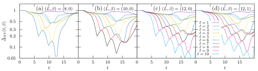
Figure S1: The value of $\Delta$ for the XY model with $(L,\beta)=$ (a) $(8,0)$, (b) $(10,0)$, (c) $(12,0)$, and (d) $(12,1)$.

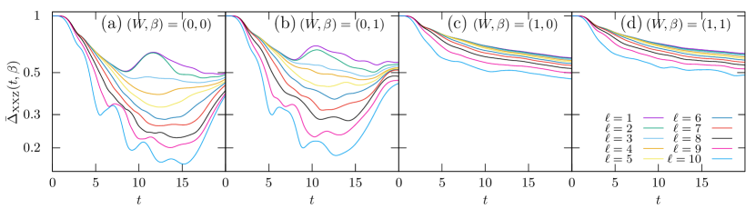
Figure S2: The value of $\bar{\Delta}$ for the XXZ model with $J_{z}=1$, $L=10$ and $(W,\beta)=$ (a) $(0,0)$, (b) $(0,1)$, (c) $(1,0)$, and (d) $(1,1)$. For (c) and (d), averages over 16 samples are plotted for $W>0$.

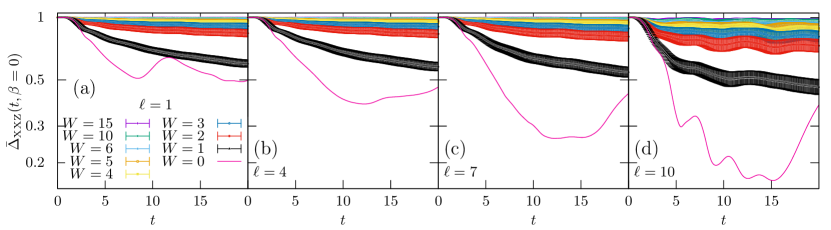
Figure S3: The value of $\bar{\Delta}$ for the XXZ model with $J_{z}=1$, $L=12$, $\beta=0$ for various values of $W$ and (a) $\ell=1$, (b) $\ell=4$, (c) $\ell=7$, and (d) $\ell=10$. Averages over 16 samples are plotted for $W>0$.

In Fig. S2, we plot the time dependence of $\bar{\Delta}$ for the XXZ model with $J=1$. For $W=0$, this is the Heisenberg model, which is integrable. Again, the plots are not converging. For $W=1$, the average over $128$ samples is plotted. The late-time behavior of the averaged value of $\bar{\Delta}$ is smoother compared to the $W=0$ case. The value decreases as $l$ is increased. (For $l=9=L-1$, we always obtain $\bar{\Delta}=0$, because the system is in the $S^{z}=0$ subspace.)

In Fig. S3, we plot the sample average of $\bar{\Delta}$ for various values of $l$ and $W$. $\bar{\Delta}$ monotonically increases and approaches unity as $W$ is increased.

We numerically observe that as $W$ is increased, $\overline{\Delta}$ monotonically increases. Even though a small $W$ introduces a chaotic behavior to the integrable spin chain at $W=0$, we conclude this does not lead to successful quantum error correction.

S5 Ising model with uniform magnetic field

A translationally invariant spin chain with nearest-neighbor Ising-type interaction and magnetic field,

$$\hat{H}_{\mathrm{Ising}}=-\sum_{j=1}^{L-1}\left(S_{j}^{z}S_{j+1}^{z}\right)-g\sum_{j=1}^{L}S_{j}^{x}-h\sum_{j=1}^{L}S_{j}^{z},$$ (S48)

is exactly solvable if $g=0$ or $h=0$. For other choices of $(g,h)$, the model is non-integrable, and the case with $(g,h)=(1.05,0.5)$ [83] has been often studied as a prototypical model of chaotic spin chain. In Fig. S4 we plot the value of $\Delta$ for $\beta=0$ and various $\ell$. We observe that while $\Delta$ decreases as $\ell$ is increased, the decrease is very slow. For finite $\beta$, the value of $\Delta$ is generally larger, indicating less efficient error correction.

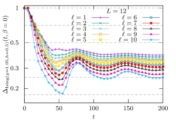
Figure S4: Ising spin chain, open boundary condition, $L=12$, $(g,h)=(1.05,0.5)$.

S6 Pure SYK₄

Here, we study the Hayden-Preskill recovery in $\mathrm{SYK}_{4}$ in detail. The original SYK model with all-to-all four fermion interactions among $2{N_{\mathrm{q}}}$ Majorana fermions is henceforth denoted as the $\mathrm{SYK}_{4}$ model. The Hamiltonian is

$$\hat{H}_{\mathrm{SYK}_{4}}=\sum_{1\leq a_{1}<a_{2}<a_{3}<a_{4}\leq 2{N_{\mathrm{q}}}}J_{a_{1}a_{2}a_{3}a_{4}}\hat{\psi}_{a_{1}}\hat{\psi}_{a_{2}}\hat{\psi}_{a_{3}}\hat{\psi}_{a_{4}},$$ (S49)

in which the $2{N_{\mathrm{q}}}$ Majorana fermions $\{\hat{\psi}_{j}\}_{j=1}^{2{N_{\mathrm{q}}}}$ satisfy the anti-commutation relation $\{\hat{\psi}_{j},\hat{\psi}_{k}\}=\hat{\psi}_{j}\hat{\psi}_{k}+\hat{\psi}_{k}\hat{\psi}_{j}=2\delta_{jk}$, in which $\delta_{ij}$ is the Kronecker delta. The time-independent real couplings $J_{a_{1}a_{2}a_{3}a_{4}}$ obey the Gaussian distribution $P(\{J_{a_{1}a_{2}a_{3}a_{4}}\})=\exp[-J_{a_{1}a_{2}a_{3}a_{4}}^{2}/2\sigma^{2}]/\sqrt{2\pi\sigma^{2}}$ with the variance $\sigma^{2}$. As $\Tr[\hat{H}_{\mathrm{SYK}_{4}}^{2}]=\sum_{1\leq a_{1}<a_{2}<a_{3}<a_{4}\leq 2N}J_{a_{1}a_{2}a_{3}a_{4}}^{2}$, we choose

$$\sigma^{2}=\binom{2{N_{\mathrm{q}}}}{4}^{-1}=\frac{12}{N(2{N_{\mathrm{q}}}-1)(2{N_{\mathrm{q}}}-2)(2{N_{\mathrm{q}}}-3)},$$ (S50)

so as to set the variance of the many-body energy eigenvalue to unity. The corresponding recovery error is denoted by $\bar{\Delta}_{\mathrm{SYK}_{4}}(t,\beta)$.

S6.1 Effectively canceling the parity symmetry

The SYK₄ model has symmetry, which divides the system into odd and even parity sectors. Accordingly, the time evolution operator is decomposed as

$$\hat{U}_{{\rm SYK}_{4}}(t)=\hat{U}_{{\rm SYK}_{4},{\rm odd}}(t)\oplus\hat{U}_{{\rm SYK}_{4},{\rm even}}(t),$$ (S51)

where $\hat{U}_{{\rm SYK}_{4},p}(t)$ ($p={\rm even},{\rm odd}$) is the unitary acting only on the sector with parity $p$. Since the presence of symmetry is known to induce drastic changes in the Hayden-Preskill recovery [10, 9, 24, 90], which we would like to ignore in this analysis, we provide a slight modification that allows us to effectively cancel the effect of symmetry.

The modification is to embed the system $A$ of $k$ qubits into an even-parity sector of a larger system $A^{\prime}$, whose Hilbert space is ${\mathcal{H}}^{A^{\prime}}:={\mathcal{H}}^{a}\otimes{\mathcal{H}}^{A}$ with ${\mathcal{H}}^{a}$ being a two-dimensional space ${\rm span}\{\ket{o},\ket{e}\}$ that labels the parity in $A^{\prime}$. For instance, when $k=1$,

—e⟩^a ⊗—0⟩^A = —00⟩^A’, —e⟩^a ⊗—1⟩^A = —11⟩^A’, —o⟩^a ⊗—0⟩^A = —01⟩^A’, and —o⟩^a ⊗—1⟩^A = —10⟩^A’. (S52)

The maximally entangled state between $A$ and $R$ is embedded to $\ket{\Phi}^{A^{\prime}R}:=\ket{e}^{a}\otimes\ket{\Phi}^{AR}$, which is a pure state in the $2^{2k+1}$-dimensional system $A^{\prime}$ with Schmidt rank $2^{k}$.

Embedding $A$ into $A^{\prime}$ enlarges the whole system $S$ to $S^{\prime}:=A^{\prime}B$ of ${N_{\mathrm{q}}}=N+1$ qubits, which we similarly decompose as $S^{\prime}=sS$, where $s$ is the two-dimensional space for labeling the parity of $S$. The time-evolution operator in $S^{\prime}$ by $\hat{U}_{{\rm SYK}_{4}}^{S^{\prime}}(t)$ is then given by

$$\hat{U}_{{\rm SYK}_{4}}^{S^{\prime}}(t)=\outerproduct{o}{o}^{s}\otimes\hat{U}_{{\rm SYK}_{4},{\rm odd}}^{S}(t)+\outerproduct{e}{e}^{s}\otimes\hat{U}_{{\rm SYK}_{4},{\rm even}}^{S}(t).$$ (S53)

Assuming that the initial thermal state $\xi(\beta)^{B}$ is in the even-parity sector, which is $2^{N-k-1}$ dimensional, the state after the time evolution is

$$\Psi^{S^{\prime}R}(t,\beta) :=\hat{U}^{S^{\prime}}_{{\rm SYK}_{4}}(t)(\Phi^{A^{\prime}R}\otimes\xi(\beta)^{B})\hat{U}^{S^{\prime}\dagger}_{{\rm SYK}_{4}}(t)$$

$$=\outerproduct{e}{e}^{s}\otimes\hat{U}^{S}_{{\rm SYK}_{4},{\rm even}}(t)\bigl{(}\Phi^{AR}\otimes\xi(\beta)^{B}\bigr{)}\hat{U}^{S\dagger}_{{\rm SYK}_{4},{\rm even}}(t).$$ (S54)

Assuming that the information that the support of the state $\Psi^{S^{\prime}R}(t,\beta)$ is the even-parity sector of ${\mathcal{H}}^{S^{\prime}}$ is available in the decoding process, the state relevant to the degree of decoupling is the one in which $s$ and $C$ are traced over:

$$\Psi^{DR}(t,\beta) =\Tr_{s,C}\bigl{[}\Psi^{S^{\prime}R}(t,\beta)\bigr{]}$$

$$=\Tr_{C}\bigl{[}\hat{U}^{S}_{{\rm SYK}_{4},{\rm even}}(t)(\Phi^{AR}\otimes\xi(\beta)^{B})\hat{U}^{S\dagger}_{{\rm SYK}_{4},{\rm even}}(t)\bigr{]}.$$ (S55)

In this way, the effect of symmetry of the SYK₄ model is effectively canceled.

It should be emphasized that this modification leads to a slight change in the degree of decoupling, resulting in a slight change of the upper bound $\bar{\Delta}$ on the recovery error. To see this, we consider the degree of decoupling when $\hat{U}^{S}_{{\rm SYK}_{4},even}(t)$ in Eq. (S55) is replaced with the Haar random unitary $U^{S}_{\rm Haar}$ acting on the even-parity sector, whose dimension is $2^{N-k-1}$. We denote it by $\Sigma^{\prime}_{\rm Haar}$. Since the system $s$, storing the parity information of $S^{\prime}$, is traced out, the state $\tau$ in Eq. (S26) changes into the state in the system $S^{\prime}\tilde{D}$ such as

$$\tau^{S^{\prime}\tilde{D}}=\Tr_{\tilde{s},\tilde{C}}\bigl{[}\outerproduct{\Phi}{\Phi}^{S^{\prime}\tilde{S}^{\prime}}\bigr{]}=\frac{I^{s}}{2}\otimes\frac{I^{C}}{2^{\ell}}\otimes\outerproduct{\Phi}{\Phi}^{D\tilde{D}}.$$ (S56)

By computing the conditional collision entropy of this state, we have

$$\log[2\Sigma^{\prime}_{\rm Haar}(\beta)]\leq\frac{N+k-H(\beta)-1}{2}-\ell.$$ (S57)

This leads to

$$\Delta^{\prime}_{\rm Haar}(\beta)\leq 2^{\frac{1}{2}\bigl{(}\frac{N+k-H(\beta)-1}{2}-\ell\bigr{)}}=2^{\frac{1}{2}\bigl{(}\frac{N+k-H(\beta)}{2}-\ell\bigr{)}-\frac{1}{4}}.$$ (S58)

This differs from Eq. (3) by $2^{-\frac{1}{4}}$, which arises from the fact that the information about the parity sector is available in the decoding process. Note also that, since we have restricted the initial thermal state $\xi(\beta)^{B}$ on the even-parity sector, its entropy also changes. For instance, its maximum value is $N-k-1$ rather than $N-k$.

S6.2 Recovery errors in the $\mathrm{SYK}_{4}$ model

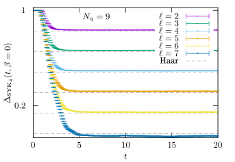
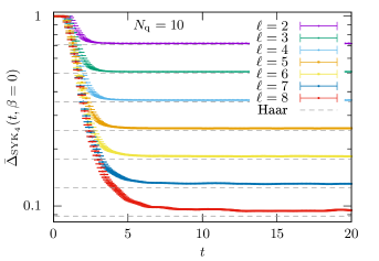
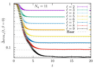
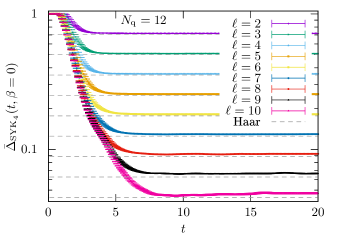
Figure S5: Semilogarithmic plot of the value of $\bar{\Delta}_{\hat{H}_{\mathrm{SYK}_{4}}}(t,\beta=0)$ against $t$ for $k=1,{N_{\mathrm{q}}}=9,10,11,12$ and $2\leq l<{N_{\mathrm{q}}}-k$. Average over $2^{19-{N_{\mathrm{q}}}}$ samples is taken. For $\ell=1$, $\bar{\Delta}_{\hat{H}_{\mathrm{SYK}_{4}}}(t,\beta=0)$ is $\sim 1$ for all $t$. The dashed lines represent $\bar{\Delta}_{\rm Haar}(\beta=0)=2^{\frac{1}{2}(1-\ell)}$ given in Eq. (3) for $\ell=2,3,\ldots,{N_{\mathrm{q}}}-2$. See Fig. 3 for the plot for ${N_{\mathrm{q}}}=13$.

The collision entropy of $\xi_{B}(\beta)$ is

$$H(\beta)=-\log\Tr[\rho(\beta)^{2}]=-\log\Tr\frac{[e^{-2\beta H}]}{Z(\beta)^{2}}=-\log\frac{Z(2\beta)}{Z(\beta)^{2}}=2\log Z(\beta)-\log Z(2\beta)=\frac{1}{\ln 2}(F(2\beta)-2F(\beta)),$$ (S59)

in which $F(\beta)=-\ln Z(\beta)$ is the Helmholtz free energy. For $\beta=0$, $Z(\beta=0)$ is simply the dimension of the Hilbert space of $B$, and we have $H(\beta=0)=\log Z(\beta=0)=N-k-1$. Therefore, the right-hand side of (S58) is

$$2^{\frac{1}{2}\bigl{(}\frac{N+k-(N-k-1)}{2}-\ell\bigr{)}-\frac{1}{4}}=2^{\frac{k-\ell}{2}};\ \bar{\Delta}^{\prime}_{\rm Haar}(\beta=0)=\min\{1,2^{\frac{k-\ell}{2}}\}.$$ (S60)

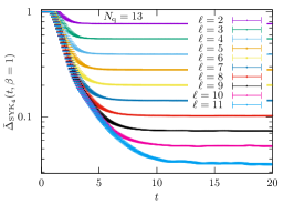
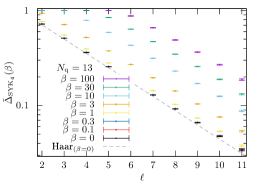
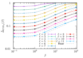
Figure S6: Left: Semilogrithmic plot of the value of $\bar{\Delta}_{\hat{H}_{\mathrm{SYK_{4}}}}(t,\beta=1)$ against $t$ for $k=1,{N_{\mathrm{q}}}=13$. For $\beta=0$, see Fig. 3 in the main text. Center: Late-time value of $\bar{\Delta}_{\hat{H}_{\mathrm{SYK_{4}}}}(t,\beta)$ averaged over $64$ samples plotted against $\ell$ for ${N_{\mathrm{q}}}=13$. Right: Late-time value $\bar{\Delta}_{\hat{H}_{\mathrm{SYK_{4}}}}(t,\beta)$ averaged over $64$ samples plotted against $\beta$ for ${N_{\mathrm{q}}}=13$. Dashed lines represent $\bar{\Delta}^{\prime}_{\mathrm{Haar}}(\beta)$.

In Fig. S5, we plot upper bound $\bar{\Delta}_{\mathrm{SYK}_{4}}$ on the recovery error against time $t$ for various $\ell$, for $9\leq{N_{\mathrm{q}}}\leq 12$ and infinite temperature $\beta=0$. Since the $\mathrm{SYK}_{4}$ model has randomness of choosing the coupling constant $J_{a_{1}a_{2}a_{3}a_{4}}$, we take an average over many samples. We clearly observe that all curves rapidly decay and approach the bound $\bar{\Delta}_{\rm Haar}$ for the Haar random dynamics, indicating that the Hayden-Preskill recovery is quickly achieved by the dynamics of $\mathrm{SYK}_{4}$. This is also the case for finite temperature, as observed in Fig. S6. The late-time value of $\bar{\Delta}_{\mathrm{SYK}_{4}}$ is in proportion to $2^{-H(\beta)/4}$ as expected from (S58) for $\beta\lesssim 10$, beyond which small deviations occur presumably due to the small number of eigenenergies within $1/\beta$ of the ground state.

Note that the $\mathrm{SYK}_{4}$ model has a ${N_{\mathrm{q}}}\mod 4$ periodicity, depending on which the eigenenergy statistics resembles the Gaussian Unitary, Orthogonal, and Symplectic Ensembles (GUE, GOE, and GSE). We have checked that this periodicity does not affect much on the Hayden-Preskill recovery, implying that the Hayden-Preskill recovery is achieved by those ensembles of random Hermitian matrices. This might be of interest since the dynamics generated by GUE, GOE, and GSE is not Haar random, but achieves the Hayden-Preskill recovery that was shown based on a Haar random unitary.

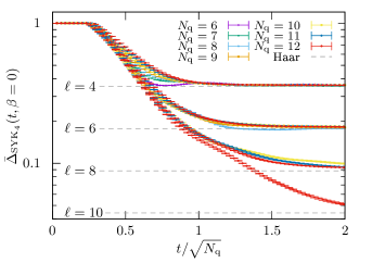
Figure S7: $\bar{\Delta}_{\hat{H}_{\mathrm{SYK}_{4}}}(t,\beta=0)$ plotted against $t/\sqrt{{N_{\mathrm{q}}}}$, for $\ell=4,6,8,10$ from top to bottom. Average over $2^{19-{N_{\mathrm{q}}}}$ samples is taken. The curves show better agreement as $\ell$ is increased, which is not observed for other choices of the exponent of ${N_{\mathrm{q}}}$ for scaling.

S6.3 Convergence time

To check the time scale needed for $\bar{\Delta}_{\mathrm{SYK}_{4}}$ converging to $\bar{\Delta}_{\rm Haar}$, we plot in Fig. S7 $\bar{\Delta}(t,\beta=0)$ for $\ell=4,6,8,10$ against re-scaled time $t/\sqrt{{N_{\mathrm{q}}}}$. The plot indicates that the convergence time is likely to be $\sqrt{{N_{\mathrm{q}}}}$.

S7 Sparse SYK₄

We consider the sparse $\mathrm{SYK}_{4}$ model [91, 92, 93], referred to as $\mathrm{spSYK}_{4}$. The model has a parameter ${K_{\mathrm{cpl}}}$ that counts the number of non-zero coupling constant $J_{a_{1}a_{2}a_{3}a_{4}}$ in Eq. (4). Other than that, the Hamiltonian of $\mathrm{spSYK}_{4}$ is defined similarly to that of $\mathrm{SYK}_{4}$. When ${K_{\mathrm{cpl}}}=\binom{{N_{\mathrm{q}}}}{4}$, then $\mathrm{spSYK}_{4}$ reduces to $\mathrm{SYK}_{4}$. Note that this approach to reducing the number of non-zero parameter is drastically different from the approach in [Dumitriu_2002], where tridiagonal matrix models generalizing the Gaussian and Wishart dense matrix models were introduced. The $\mathrm{SYK}_{4}$ Hamiltonian is still sparse when presented as a matrix in the many-body Hilbert space.

For simpliity, we further introduce a constraint that a half of the non-zero couplings is set to $1/\sqrt{{K_{\mathrm{cpl}}}}$ and the other half is $-1/\sqrt{{K_{\mathrm{cpl}}}}$, which we call $\pm\mathrm{spSYK}_{4}$ model. The corresponding upper bound of the recovery error is denoted by $\bar{\Delta}_{\pm\mathrm{spSYK}_{4}}(t,\beta)$ for time $t$ and the inverse temperature $\beta$.

The sparse $\mathrm{SYK}_{4}$ model is known to have a transition from quantum chaos to integrability by varying the number ${K_{\mathrm{cpl}}}$ of non-zero coupling constant. For ${K_{\mathrm{cpl}}}\ll 2{N_{\mathrm{q}}}$, we typically have extra degeneracy in the spectrum than expected from the symmetry, and the spectral statistics of the distinct eigenvalues is not random-matrix like. For ${K_{\mathrm{cpl}}}\gtrsim 2{N_{\mathrm{q}}}$, such extra degeneracy disappears for practically all samples, and the spectral statistics strongly resembles that of the Gaussian random matrix ensemble with the corresponding symmetry [91, 92, 93]. It is surprising to some extent that the $\pm\mathrm{spSYK}_{4}$ recovers important properties of $\mathrm{SYK}_{4}$ when ${K_{\mathrm{cpl}}}=O(N)$, which is by far smaller than ${K_{\mathrm{cpl}}}=\binom{{N_{\mathrm{q}}}}{4}$, which is needed for $\hat{H}_{\mathrm{spSYK}_{4}}$ reducing to $\hat{H}_{\mathrm{SYK}_{4}}$.

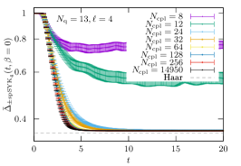
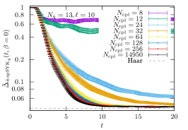
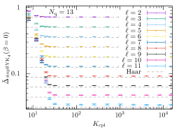
Figure S8: The value of $\bar{\Delta}_{\pm\mathrm{spSYK}_{4}}(t,\beta=0)$ plotted against $t$ for $k=1,{N_{\mathrm{q}}}=13$ and $\ell=4$ (left), $\ell=10$ (center). 64 samples are used. The result for the $\mathrm{SYK}_{4}$ model as well as the Haar value, $\bar{\Delta}_{\rm Haar}(\beta=0)=2^{\frac{1-\ell}{2}}$, are also shown. (right) The late-time value of $\bar{\Delta}_{\pm\mathrm{spSYK}_{4}}(t,\beta=0)$ plotted for ${N_{\mathrm{q}}}=13$, $k=1$, and various $\ell$ against the number ${K_{\mathrm{cpl}}}$ of nonzero couplings. 64 samples are used.

In Fig. S8(a–b), we plot $\bar{\Delta}_{\pm\mathrm{spSYK}_{4}}(t,\beta)$ for $\ell=4,10$ against $t$ for various values of ${K_{\mathrm{cpl}}}$. At an earlier time, $\bar{\Delta}_{\pm\mathrm{spSYK}_{4}}(t,\beta)$ starts decreasing for any ${K_{\mathrm{cpl}}}(>0)$ as time $t$ increases, which is similar to the $\mathrm{SYK}_{4}$ model, but it soon witnesses the difference from $\mathrm{SYK}_{4}$ when ${K_{\mathrm{cpl}}}$ is small. For ${K_{\mathrm{cpl}}}\lesssim 16$, $\bar{\Delta}_{\pm\mathrm{spSYK}_{4}}$ is unlikely to converge to the Haar value $\bar{\Delta}_{\rm Haar,th}$ even in the large time limit, while for large ${K_{\mathrm{cpl}}}$, $\bar{\Delta}_{\pm\mathrm{spSYK}_{4}}$ seems to eventually converge to $\bar{\Delta}_{\rm Haar,th}$ as $t$ increases. Hence, we observe from these plots that at least two differences come up in the $\pm\mathrm{spSYK}_{4}$ model in comparison with the $\mathrm{SYK}_{4}$ model. One is the converging value of $\bar{\Delta}_{\pm\mathrm{spSYK}_{4}}(t=\infty,\beta)$, and the other is the time scale for convergence.

To closely investigate the converging value, we plot in Fig. S8(c) the late-time value of $\bar{\Delta}_{\pm\mathrm{spSYK}_{4}}$ for various $\ell$ against ${K_{\mathrm{cpl}}}$ for $2{N_{\mathrm{q}}}=26$ Majorana fermions. It is clear that the value is nearly identical to the Haar value for ${K_{\mathrm{cpl}}}\gtrsim 30$. This convergence to the dense SYK limit is consistent with the eigenenergy statistics.[93] For the density of states plotted in the left panel of Fig. S9, we observe that while the overall shape stays similar, the fluctuation disappears as we increase ${K_{\mathrm{cpl}}}$. The fluctuation observed for smaller ${K_{\mathrm{cpl}}}$ originates from the decrease in the number of distinct eigenvalues due to the additional degeneracy when emergent conserved quantities appear.[92, 93]

S8 SYK₄₊₂

Because the trace of the product of six Majorana fermions is zero when four of them differ with each other, for the SYK₄₊₂ model defined in eq. (5), we have

$$\Tr\hat{H}_{\mathrm{SYK}_{4+2}}(\theta)^{2}=(\cos^{2}\theta)\Tr\hat{H}_{\mathrm{SYK}_{4}}^{2}+(\sin^{2}\theta)\Tr\hat{H}_{\mathrm{SYK}_{2}}^{2}=2^{N_{\mathrm{q}}}.$$ (S61)

Note that the normalization in [48] is so that $\hat{H}_{\mathrm{SYK}_{4+2}}(\theta)=\hat{H}_{\mathrm{SYK}_{4}}+\delta\hat{H}_{\mathrm{SYK}_{2}}$ with the variance of the many-body eigenvalues for $\hat{H}_{\mathrm{SYK}_{4}}$ is $24(2{N_{\mathrm{q}}})^{-4}\begin{pmatrix}2{N_{\mathrm{q}}}\\ 4\end{pmatrix}\sim 1$, and the variance of the single-particle eigenvalues for $\hat{H}_{\mathrm{SYK}_{2}}$ is $\delta^{2}(2{N_{\mathrm{q}}})^{-3}(2{N_{\mathrm{q}}}-2)(2{N_{\mathrm{q}}}-3)\sim\delta^{2}/(2{N_{\mathrm{q}}})$.

S8.1 The density of states for SYK₄₊₂

We plot in the right panel of Fig. S9 the density of states for various values of $\tan\theta$. The variance of the eigenstate energy is fixed at unity. As $\tan\theta$ is increased, the peak becomes higher and the tails become thicker, changing from a RMT-like spectrum, which is a sign for quantum chaos and is the case for SYK₄, to a Gaussian-shape spectrum, which differs from SYK₄.

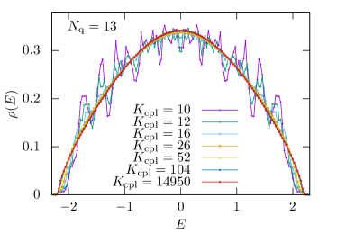
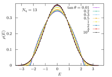
Figure S9: The normalized density of states for (left) $\hat{H}_{\pm\mathrm{spSYK}_{4}}$ plotted for ${N_{\mathrm{q}}}=13$ and 2048 samples, and for (right) $\hat{H}_{\mathrm{SYK}_{4+2}}$ plotted for ${N_{\mathrm{q}}}=13$ and 64 samples.

S8.2 Numerical results for SYK₄₊₂

We here provide numerical results of the Hayden-Preskill recovery in the $\mathrm{SYK}_{4+2}$ model. The Hamiltonian is given by

$$\hat{H}_{\mathrm{SYK}_{4+2}}(\theta) =(\cos\theta)\hat{H}_{\mathrm{SYK}_{4}}+(\sin\theta)\hat{H}_{\mathrm{SYK}_{2}}$$

$$=(\cos\theta)\left(\hat{H}_{\mathrm{SYK}_{4}}+(\tan\theta)\hat{H}_{\mathrm{SYK}_{2}}\right),$$ (5)

which maps to the normalization in [48] by $\delta=\tan\theta$. The $\mathrm{SYK}_{4+2}$ model trivially reduces to $\mathrm{SYK}_{4}$ when $\delta=0$. Below, we denote by $\bar{\Delta}_{\mathrm{SYK}_{4+2}}(t,\beta)$ the corresponding upper bound on the recovery error and investigate it.

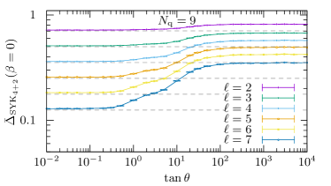
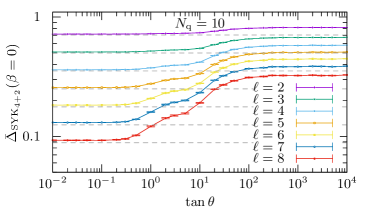
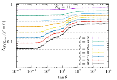
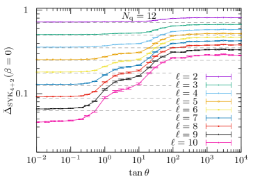
Figure S10: The value of $\bar{\Delta}_{\mathrm{SYK}_{4+2}}(t,\beta=0)$ plotted for $k=1$ and various $\ell$ against the value of $\delta$ for ${N_{\mathrm{q}}}=9,10,11,12$. $2^{19-{N_{\mathrm{q}}}}=2^{10},2^{9},2^{8},2^{7}$ samples are used and average over the values for $t=(1,2,\ldots,10)\times 10^{6}$ is taken. The lines connecting the data points are guide to the eye.

By varying the strength $\delta$ of the $\mathrm{SYK}_{2}$ term, this Hamiltonian shows a transition from quantum chaos, in the sense of eigenenergy statistics, to Fock space many-body localization (F-MBL) at $\delta_{\mathrm{c}}\simeq{N_{\mathrm{q}}}^{2}\ln{N_{\mathrm{q}}}$ [48], which corresponds to $\tan\theta=\mathcal{O}(10^{2})$ for $9\leq{N_{\mathrm{q}}}\leq 13$ that we numerically study in this work.

In Fig. S10 we plot the late time behaviour of $\bar{\Delta}_{\mathrm{SYK}_{4+2}}(t,\beta)$ by setting $\beta=0$ as a function of the SYK₂ coupling strength $\delta=\tan\theta$. There are two characteristic values of $\delta=\tan\theta$, $\delta_{0}=\tan\theta_{0}\approx 0.1$ and $\delta_{1}=\tan\theta_{1}\approx 3$, yielding three plateau-like shapes of $\bar{\Delta}_{\mathrm{SYK}_{4+2}}$. When $0\leq\theta\leq\theta_{0}$, $\bar{\Delta}_{\mathrm{SYK}_{4+2}}\approx\bar{\Delta}_{\rm Haar}$. This implies that the Hayden-Preskill recovery in the $\mathrm{SYK}_{4}$ model is stable against small perturbations by the $\mathrm{SYK}_{2}$ terms. When $\theta_{0}\leq\theta\leq\theta_{1}$, $\bar{\Delta}_{\mathrm{SYK}_{4+2}}$ starts deviating from the Haar value $\bar{\Delta}_{\rm Haar}(\beta=0)$ and increases linearly in terms of $\delta$ until it reaches the second plateau. The second plateau ends at $\theta=\theta_{1}$ and, for $\theta\geq\theta_{1}$, $\bar{\Delta}_{\mathrm{SYK}_{4+2}}$ restarts increasing until the third plateau.

References

- Hayden and Preskill [2007] P. Hayden and J. Preskill, Black holes as mirrors: quantum information in random subsystems, J. High Energ. Phys. 0709, 120 (2007), arXiv:0708.4025 [hep-th] .
- Sekino and Susskind [2008] Y. Sekino and L. Susskind, Fast scramblers, J. High Energ. Phys. 0810, 065 (2008), arXiv:0808.2096 [hep-th] .
- Susskind [2011] L. Susskind, Addendum to Fast Scramblers (2011), arXiv:1101.6048 [hep-th] .
- Lashkari et al. [2013] N. Lashkari, D. Stanford, M. Hastings, T. Osborne, and P. Hayden, Towards the fast scrambling conjecture, J. High Energ. Phys. 1304, 022 (2013), arXiv:1111.6580 [hep-th] .
- Shenker and Stanford [2014] S. H. Shenker and D. Stanford, Black holes and the butterfly effect, J. High Energ. Phys. 1403, 067 (2014), arXiv:1306.0622 [hep-th] .
- Shenker and Stanford [2015] S. H. Shenker and D. Stanford, Stringy effects in scrambling, J. High Energ. Phys. 1505, 132 (2015), arXiv:1412.6087 [hep-th] .
- Roberts and Stanford [2015] D. A. Roberts and D. Stanford, Diagnosing Chaos Using Four-Point Functions in Two-Dimensional Conformal Field Theory, Phys. Rev. Lett. 115, 131603 (2015), arXiv:1412.5123 [hep-th] .
- Roberts and Yoshida [2017] D. A. Roberts and B. Yoshida, Chaos and complexity by design, J. High Energ. Phys. 1704, 121 (2017), arXiv:1610.04903 [quant-ph] .
- Yoshida [2019] B. Yoshida, Soft mode and interior operator in the Hayden-Preskill thought experiment, Phys. Rev. D 100, 086001 (2019), arXiv:1812.07353 [hep-th] .
- Liu [2020] J. Liu, Scrambling and decoding the charged quantum information, Phys. Rev. Res. 2, 043164 (2020), arXiv:2003.11425 [quant-ph] .
- Kitaev [2015a] A. Kitaev, “Hidden correlations in the Hawking radiation and thermal noise.”, talk at KITP (2015a), http://online.kitp.ucsb.edu/online/joint98/kitaev/.
- Kitaev [2015b] A. Kitaev, “A simple model of quantum holography.”, talks at KITP (2015b), http://online.kitp.ucsb.edu/online/entangled15/kitaev/ and http://online.kitp.ucsb.edu/online/entangled15/kitaev2/.
- Jensen [2016] K. Jensen, Chaos in AdS2 Holography, Phys. Rev. Lett. 117, 111601 (2016), arXiv:1605.06098 [hep-th] .
- Maldacena and Stanford [2016] J. Maldacena and D. Stanford, Remarks on the Sachdev-Ye-Kitaev model, Phys. Rev. D 94, 106002 (2016), arXiv:1604.07818 [hep-th] .
- Sachdev [2015] S. Sachdev, Bekenstein-Hawking Entropy and Strange Metals, Phys. Rev. X 5, 041025 (2015), arXiv:1506.05111 [hep-th] .
- Blake [2016] M. Blake, Universal Charge Diffusion and the Butterfly Effect in Holographic Theories, Phys. Rev. Lett. 117, 091601 (2016), arXiv:1603.08510 [hep-th] .
- von Keyserlingk et al. [2018] C. W. von Keyserlingk, T. Rakovszky, F. Pollmann, and S. L. Sondhi, Operator Hydrodynamics, OTOCs, and Entanglement Growth in Systems without Conservation Laws, Phys. Rev. X 8, 021013 (2018), arXiv:1705.08910 [cond-mat.str-el] .
- Khemani et al. [2018] V. Khemani, A. Vishwanath, and D. A. Huse, Operator Spreading and the Emergence of Dissipative Hydrodynamics under Unitary Evolution with Conservation Laws, Phys. Rev. X 8, 031057 (2018), arXiv:1710.09835 [cond-mat.stat-mech] .
- Hosur et al. [2016] P. Hosur, X.-L. Qi, D. A. Roberts, and B. Yoshida, Chaos in quantum channels, J. High Energ. Phys. 1602, 004 (2016), arXiv:1511.04021 [hep-th] .
- Pastawski et al. [2015] F. Pastawski, B. Yoshida, D. Harlow, and J. Preskill, Holographic quantum error-correcting codes: toy models for the bulk/boundary correspondence, J. High Energ. Phys. 1506, 149 (2015), arXiv:1503.06237 [hep-th] .
- Pastawski et al. [2017] F. Pastawski, J. Eisert, and H. Wilming, Towards Holography via Quantum Source-Channel Codes, Phys. Rev. Lett. 119, 020501 (2017), arXiv:1611.07528 [quant-ph] .
- Kohler and Cubitt [2019] T. Kohler and T. Cubitt, Toy models of holographic duality between local Hamiltonians, J. High Energ. Phys. 1908, 017 (2019), arXiv:1810.08992 [hep-th] .
- Hayden and Penington [2019] P. Hayden and G. Penington, Learning the Alpha-bits of black holes, J. High Energ. Phys. 1912, 007 (2019), arXiv:1807.06041 [hep-th] .
- Nakata et al. [2023] Y. Nakata, E. Wakakuwa, and M. Koashi, Black holes as clouded mirrors: the Hayden-Preskill protocol with symmetry, Quantum 7, 928 (2023), arXiv:2007.00895 [quant-ph] .
- Nakata et al. [2022] Y. Nakata, T. Matsuura, and M. Koashi, Constructing quantum decoders based on complementarity principle (2022), arXiv:2210.06661 [quant-ph] .
- Cheng et al. [2020] Y. Cheng, C. Liu, J. Guo, Y. Chen, P. Zhang, and H. Zhai, Realizing the Hayden-Preskill protocol with coupled Dicke models, Phys. Rev. Res. 2, 043024 (2020), arXiv:1909.12568 [cond-mat.quant-gas] .
- Landsman et al. [2019] K. A. Landsman, C. Figgatt, T. Schuster, N. M. Linke, B. Yoshida, N. Y. Yao, and C. Monroe, Verified quantum information scrambling, Nature 567, 61 (2019), arXiv:1806.02807 [quant-ph] .
- Brown et al. [2023] A. R. Brown, H. Gharibyan, S. Leichenauer, H. W. Lin, S. Nezami, G. Salton, L. Susskind, B. Swingle, and M. Walter, Quantum Gravity in the Lab. I. Teleportation by Size and Traversable Wormholes, PRX Quantum 4, 010320 (2023), arXiv:1911.06314 [quant-ph] .
- Nezami et al. [2023] S. Nezami, H. W. Lin, A. R. Brown, H. Gharibyan, S. Leichenauer, G. Salton, L. Susskind, B. Swingle, and M. Walter, Quantum Gravity in the Lab. II. Teleportation by Size and Traversable Wormholes, PRX Quantum 4, 010321 (2023), arXiv:2102.01064 [quant-ph] .
- Hawking [1974] S. W. Hawking, Black hole explosions?, Nature 248, 30 (1974).
- Hawking [1975] S. W. Hawking, Particle creation by black holes, Commun. Math. Phys. 43, 199 (1975).
- Hawking [1976] S. W. Hawking, Breakdown of predictability in gravitational collapse, Phys. Rev. D 14, 2460 (1976).
- Haake [2001] F. Haake, Quantum Signatures of Chaos (Springer, Berlin, Heidelberg, 2001).
- Mehta [2004] M. Mehta, Random Matrices (Elsevier Science, 2004).
- [35] P. Caputa, J. Simón, A. Štikonas, T. Takayanagi, and K. Watanabe, Scrambling time from local perturbations of the eternal BTZ black hole, J. High Energ. Phys. 1508, 011, arXiv:1503.08161 [hep-th] .
- Nie et al. [2019] L. Nie, M. Nozaki, S. Ryu, and M. T. Tan, Signature of quantum chaos in operator entanglement in 2d CFTs, J. Stat. Mech. 2019, 093107 (2019), arXiv:1812.00013 [hep-th] .
- Goto et al. [2023] K. Goto, M. Nozaki, S. Ryu, K. Tamaoka, and M. T. Tan, Scrambling and Recovery of Quantum Information in Inhomogeneous Quenches in Two-dimensional Conformal Field Theories (2023), arXiv:2302.08009 [hep-th] .
- Larkin and Ovchinnikov [1969] A. I. Larkin and Y. N. Ovchinnikov, Quasiclassical Method in the Theory of Superconductivity, Sov. Phys. JETP 28, 1200 (1969).
- Shen et al. [2017] H. Shen, P. Zhang, R. Fan, and H. Zhai, Out-of-Time-Order Correlation at a Quantum Phase Transition, Phys. Rev. B 96, 054503 (2017), arXiv:1608.02438 [cond-mat.quant-gas] .
- Sachdev and Ye [1993] S. Sachdev and J. Ye, Gapless spin-fluid ground state in a random quantum Heisenberg magnet, Phys. Rev. Lett. 70, 3339 (1993), arXiv:cond-mat/9212030 .
- Sachdev [2010] S. Sachdev, Holographic Metals and the Fractionalized Fermi Liquid, Phys. Rev. Lett. 105, 151602 (2010), arXiv:1006.3794 [hep-th] .
- Cotler et al. [2017] J. S. Cotler, G. Gur-Ari, M. Hanada, J. Polchinski, P. Saad, S. H. Shenker, D. Stanford, A. Streicher, and M. Tezuka, Black Holes and Random Matrices, J. High Energ. Phys. 1705, 118 (2017), arXiv:1611.04650 [hep-th] .
- Sarosi [2018] G. Sarosi, AdS2 holography and the SYK model, in Proceedings of XIII Modave Summer School in Mathematical Physics — PoS(Modave2017) (Sissa Medialab, 2018) arXiv:1711.08482 [hep-th] .
- Trunin [2021] D. A. Trunin, Pedagogical introduction to the Sachdev–Ye–Kitaev model and two-dimensional dilaton gravity, Physics-Uspekhi 64, 219 (2021), arXiv:2002.12187 [hep-th] .
- Maldacena et al. [2016] J. Maldacena, S. H. Shenker, and D. Stanford, A bound on chaos, J. High Ener. Phys. 1608, 106 (2016), arXiv:1503.01409 [hep-th] .
- Bohigas et al. [1984] O. Bohigas, M. J. Giannoni, and C. Schmit, Characterization of chaotic quantum spectra and universality of level fluctuation laws, Phys. Rev. Lett. 52, 1 (1984).
- Sachdev [2022] S. Sachdev, Statistical mechanics of strange metals and black holes, ICTS Newsletter 8, 1 (2022), arXiv:2205.02285 [hep-th] .
- Monteiro et al. [2021a] F. Monteiro, T. Micklitz, M. Tezuka, and A. Altland, Minimal model of many-body localization, Phys. Rev. Res. 3, 013023 (2021a), arXiv:2005.12809 [cond-mat.str-el] .
- Monteiro et al. [2021b] F. Monteiro, M. Tezuka, A. Altland, D. A. Huse, and T. Micklitz, Quantum Ergodicity in the Many-Body Localization Problem, Phys. Rev. Lett. 127, 030601 (2021b), arXiv:2012.07884 [cond-mat.dis-nn] .
- Balasubramanian et al. [2023] V. Balasubramanian, A. Kar, C. Li, O. Parrikar, and H. Rajgadia, Quantum Error Correction from Complexity in Brownian SYK (2023), arXiv:2301.07108 [hep-th] .
- [51] J. Cotler, N. Hunter-Jones, J. Liu, and B. Yoshida, Chaos, complexity, and random matrices, J. High Energ. Phys. 2017, 48, arXiv:1706.05400 [hep-th] .
- Xu and Swingle [2022] S. Xu and B. Swingle, Scrambling Dynamics and Out-of-Time Ordered Correlators in Quantum Many-Body Systems: a Tutorial (2022), arXiv:2202.07060 [quant-ph] .
- [53] See Supplemental Material, with additional references [95, 96, Dumitriu_2002], for the upper and lower bounds on the recovery error and additional discussions on the Hayden-Preskill recovery by a Haar random dynamics, in commuting Hamiltonian models, in the Heisenberg model with random magnetic field, in the Ising model with chaotic spin chain, in the pure SYK4 model, in the sparse SYK4 model, and in the SYK4+2 model.
- Hayden et al. [2008] P. Hayden, M. Horodecki, A. Winter, and J. Yard, A Decoupling Approach to the Quantum Capacity, Open Syst. Inf. Dyn. 15, 7 (2008), arXiv:quant-ph/0702005 .
- Dupuis et al. [2014] F. Dupuis, M. Berta, J. Wullschleger, and R. Renner, One-Shot Decoupling, Commun. Math. Phys. 328, 251 (2014), arXiv:1012.6044 [quant-ph] .
- Dupuis [2009] F. Dupuis, The decoupling approach to quantum information theory, Ph.D. thesis, Université de Montréal (2009), arXiv:1004.1641 [quant-ph] .
- Wilde [2013] M. M. Wilde, Quantum Information Theory (Cambridge University Press, 2013).
- Yoshida and Kitaev [2017] B. Yoshida and A. Kitaev, Efficient decoding for the Hayden-Preskill protocol (2017), arXiv:1710.03363 [hep-th] .
- Yoshida and Yao [2019] B. Yoshida and N. Y. Yao, Disentangling Scrambling and Decoherence via Quantum Teleportation, Phys. Rev. X 9, 011006 (2019), arXiv:1803.10772 [quant-ph] .
- Katzgraber and Krza̧kała [2007] H. G. Katzgraber and F. Krza̧kała, Temperature and Disorder Chaos in Three-Dimensional Ising Spin Glasses, Phys. Rev. Lett. 98, 017201 (2007), arXiv:cond-mat/0606180 [cond-mat.dis-nn] .
- Gur-Ari et al. [2018] G. Gur-Ari, R. Mahajan, and A. Vaezi, Does the SYK model have a spin glass phase?, J. High Energ. Phys. 1811, 070 (2018), arXiv:1806.10145 [hep-th] .
- Rodriguez-Nieva et al. [2023] J. F. Rodriguez-Nieva, C. Jonay, and V. Khemani, Quantifying quantum chaos through microcanonical distributions of entanglement (2023), arXiv:2305.11940 [cond-mat.stat-mech] .
- Santos [2004] L. F. Santos, Integrability of a disordered Heisenberg spin-1/2 chain, J. Phys. A Math. Theor. 37, 4723 (2004), arXiv:cond-mat/0310035 .
- Kudo and Deguchi [2004] K. Kudo and T. Deguchi, Level statistics of spin chains with a random magnetic field, Phys. Rev. B 69, 132404 (2004), arXiv:cond-mat/0310752 [cond-mat.stat-mech] .
- Viola and Brown [2007] L. Viola and W. G. Brown, Generalized entanglement as a framework for complex quantum systems: purity versus delocalization measures, J. Phys. A Math. Theor. 40, 8109 (2007), arXiv:quant-ph/0702014 [quant-ph] .
- Žnidarič et al. [2008] M. Žnidarič, T. Prosen, and P. Prelovšek, Many-body localization in the Heisenberg XXZ magnet in a random field, Phys. Rev. B 77, 064426 (2008), arXiv:0706.2539 [quant-ph] .
- Pal and Huse [2010] A. Pal and D. A. Huse, Many-body localization phase transition, Phys. Rev. B 82, 174411 (2010), arXiv:1010.1992 [cond-mat.dis-nn] .
- Luca and Scardicchio [2013] A. D. Luca and A. Scardicchio, Ergodicity breaking in a model showing many-body localization, EPL (Europhysics Letters) 101, 37003 (2013), arXiv:1206.2342 [cond-mat.str-el] .
- Alet and Laflorencie [2018] F. Alet and N. Laflorencie, Many-body localization: An introduction and selected topics, C. R. Phys. 19, 498 (2018), arXiv:1711.03145 [cond-mat.str-el] .
- Abanin et al. [2019] D. A. Abanin, E. Altman, I. Bloch, and M. Serbyn, Colloquium: Many-body localization, thermalization, and entanglement, Rev. Mod. Phys. 91, 021001 (2019), arXiv:1804.11065 [cond-mat.dis-nn] .
- Luitz et al. [2015] D. J. Luitz, N. Laflorencie, and F. Alet, Many-body localization edge in the random-field Heisenberg chain, Phys. Rev. B 91, 081103 (2015), arXiv:1411.0660 [cond-mat.dis-nn] .
- Morningstar and Huse [2019] A. Morningstar and D. A. Huse, Renormalization-group study of the many-body localization transition in one dimension, Phys. Rev. B 99, 224205 (2019), arXiv:1903.02001 [cond-mat.stat-mech] .
- Šuntajs et al. [2020] J. Šuntajs, J. Bonča, T. Prosen, and L. Vidmar, Quantum chaos challenges many-body localization, Phys. Rev. E 102, 062144 (2020), arXiv:1905.06345 [cond-mat.str-el] .
- Sierant et al. [2020] P. Sierant, D. Delande, and J. Zakrzewski, Thouless Time Analysis of Anderson and Many-Body Localization Transitions, Phys. Rev. Lett. 124, 186601 (2020), arXiv:1911.06221 [cond-mat.dis-nn] .
- Kiefer-Emmanouilidis et al. [2020] M. Kiefer-Emmanouilidis, R. Unanyan, M. Fleischhauer, and J. Sirker, Evidence for Unbounded Growth of the Number Entropy in Many-Body Localized Phases, Phys. Rev. Lett. 124, 243601 (2020), arXiv:2003.04849 [cond-mat.dis-nn] .
- Chanda et al. [2020] T. Chanda, P. Sierant, and J. Zakrzewski, Many-body localization transition in large quantum spin chains: The mobility edge, Phys. Rev. Res. 2, 032045 (2020), arXiv:2006.02860 [cond-mat.dis-nn] .
- Sels and Polkovnikov [2021] D. Sels and A. Polkovnikov, Dynamical obstruction to localization in a disordered spin chain, Phys. Rev. E 104, 054105 (2021), arXiv:2009.04501 [quant-ph] .
- Kiefer-Emmanouilidis et al. [2021] M. Kiefer-Emmanouilidis, R. Unanyan, M. Fleischhauer, and J. Sirker, Slow delocalization of particles in many-body localized phases, Phys. Rev. B 103, 024203 (2021), arXiv:2010.00565 [cond-mat.dis-nn] .
- Morningstar et al. [2022] A. Morningstar, L. Colmenarez, V. Khemani, D. J. Luitz, and D. A. Huse, Avalanches and many-body resonances in many-body localized systems, Phys. Rev. B 105, 174205 (2022), arXiv:2107.05642 [cond-mat.dis-nn] .
- Sels [2022] D. Sels, Bath-induced delocalization in interacting disordered spin chains, Phys. Rev. B 106, L020202 (2022), arXiv:2108.10796 [cond-mat.dis-nn] .
- Sierant and Zakrzewski [2022] P. Sierant and J. Zakrzewski, Challenges to observation of many-body localization, Phys. Rev. B 105, 224203 (2022), arXiv:2109.13608 [cond-mat.dis-nn] .
- Ghosh and Žnidarič [2022] R. Ghosh and M. Žnidarič, Resonance-induced growth of number entropy in strongly disordered systems, Phys. Rev. B 105, 144203 (2022), arXiv:2112.12987 [cond-mat.dis-nn] .
- Bañuls et al. [2011] M. C. Bañuls, J. I. Cirac, and M. B. Hastings, Strong and Weak Thermalization of Infinite Nonintegrable Quantum Systems, Phys. Rev. Lett. 106, 050405 (2011), arXiv:1007.3957 [quant-ph] .
- Li et al. [2017] J. Li, R. Fan, H. Wang, B. Ye, B. Zeng, H. Zhai, X. Peng, and J. Du, Measuring Out-of-Time-Order Correlators on a Nuclear Magnetic Resonance Quantum Simulator, Phys. Rev. X 7, 031011 (2017), arXiv:1609.01246 [cond-mat.str-el] .
- Fan et al. [2017] R. Fan, P. Zhang, H. Shen, and H. Zhai, Out-of-time-order correlation for many-body localization, Sci. Bull. 62, 707 (2017), arXiv:1608.01914 [cond-mat.quant-gas] .
- Riddell and Sørensen [2019] J. Riddell and E. S. Sørensen, Out-of-time ordered correlators and entanglement growth in the random-field XX spin chain, Phys. Rev. B 99, 054205 (2019), arXiv:1810.00038 [cond-mat.stat-mech] .
- Lee et al. [2019] J. Lee, D. Kim, and D.-H. Kim, Typical growth behavior of the out-of-time-ordered commutator in many-body localized systems, Phys. Rev. B 99, 184202 (2019), arXiv:1812.00357 [cond-mat.str-el] .
- Xu and Swingle [2020] S. Xu and B. Swingle, Accessing scrambling using matrix product operators, Nature Physics 16, 199 (2020), arXiv:1802.00801 [quant-ph] .
- Shukla et al. [2022] R. K. Shukla, A. Lakshminarayan, and S. K. Mishra, Out-of-time-order correlators of nonlocal block-spin and random observables in integrable and nonintegrable spin chains, Phys. Rev. B 105, 224307 (2022), arXiv:2203.05494 [quant-ph] .
- Tajima and Saito [2021] H. Tajima and K. Saito, Universal limitation of quantum information recovery: symmetry versus coherence (2021), arXiv:2103.01876 [quant-ph] .
- Xu et al. [2020] S. Xu, L. Susskind, Y. Su, and B. Swingle, A Sparse Model of Quantum Holography (2020), arXiv:2008.02303 [cond-mat.str-el] .
- García-García et al. [2021] A. M. García-García, Y. Jia, D. Rosa, and J. J. M. Verbaarschot, Sparse Sachdev-Ye-Kitaev model, quantum chaos, and gravity duals, Phys. Rev. D 103, 106002 (2021), arXiv:2007.13837 [hep-th] .
- Tezuka et al. [2023] M. Tezuka, O. Oktay, E. Rinaldi, M. Hanada, and F. Nori, Binary-coupling sparse Sachdev-Ye-Kitaev model: an improved model of quantum chaos and holography, Phys. Rev. B 107, L081103 (2023), arXiv:2208.12098 [quant-ph] .
- García-García et al. [2018] A. M. García-García, B. Loureiro, A. Romero-Bermúdez, and M. Tezuka, Chaotic-Integrable Transition in the Sachdev-Ye-Kitaev Model, Phys. Rev. Lett. 120, 241603 (2018), arXiv:1707.02197 [hep-th] .
- Nandy et al. [2022] D. K. Nandy, T. Čadež, B. Dietz, A. Andreanov, and D. Rosa, Delayed thermalization in the mass-deformed Sachdev-Ye-Kitaev model, Phys. Rev. B 106, 245147 (2022), arXiv:2206.08599 [cond-mat.str-el] .
- Wakakuwa and Nakata [2021] E. Wakakuwa and Y. Nakata, One-Shot Randomized and Nonrandomized Partial Decoupling, Commun. Math. Phys. 386, 589 (2021), arXiv:1903.05796 [quant-ph] .