FairShap: A Data Re-weighting Approach for
Algorithmic Fairness based on Shapley Values

Abstract

Algorithmic fairness is of utmost societal importance, yet the current trend in large-scale machine learning models requires training with massive datasets that are frequently biased. In this context, pre-processing methods that focus on modeling and correcting bias in the data emerge as valuable approaches. In this paper, we propose FairShap, a novel instance-level data re-weighting method for fair algorithmic decision-making through data valuation by means of Shapley Values. FairShap is model-agnostic and easily interpretable, as it measures the contribution of each training data point to a predefined fairness metric. We empirically validate FairShap on several state-of-the-art datasets of different nature, with a variety of training scenarios and models and show how it yields fairer models with similar levels of accuracy than the baselines. We illustrate FairShap’s interpretability by means of histograms and latent space visualizations. Moreover, we perform a utility-fairness study, and ablation and runtime experiments to illustrate the impact of the size of the reference dataset and FairShap’s computational cost depending on the size of the dataset and the number of features. We believe that FairShap represents a promising direction in interpretable and model-agnostic approaches to algorithmic fairness that yield competitive accuracy even when only biased datasets are available.

Keywords: Algorithmic Fairness, Data Valuation, Shapley Value, Instance-level Re-weighting, Model-agnostic Fairness

1 Introduction

Machine learning (ML) models are increasingly used to support human decision-making in a broad set of use cases, including in high-stakes domains, such as healthcare, education, finance, policing, or immigration. In these scenarios, algorithmic design, implementation, deployment, evaluation and auditing should be performed cautiously to minimize the potential negative consequences of their use, and to develop fair, transparent, accountable, privacy-preserving, reproducible and reliable systems (Barocas et al., 2019; Smuha, 2019; Oliver, 2022). To achieve algorithmic fairness, a variety of fairness metrics that model mathematically different definitions of equality have been proposed in the literature (Carey and Wu, 2022). Group fairness focuses on ensuring that different demographic groups are treated fairly by an algorithm (Hardt et al., 2016; Zafar et al., 2017), and individual fairness aims to give a similar treatment to similar individuals (Dwork et al., 2012). In the past decade, numerous machine learning methods have been proposed to achieve algorithmic fairness (Mehrabi et al., 2021).

Algorithmic fairness may be addressed in the three stages of the ML pipeline: first, by modifying the input data (pre-processing) via e.g. re-sampling, data cleaning, re-weighting or learning fair representations (Kamiran and Calders, 2012; Zemel et al., 2013); second, by including a fairness metric in the optimization function of the learning process (in-processing) (Zhang et al., 2018; Kamishima et al., 2012); and third, by adjusting the model’s decision threshold to ensure fair decisions across groups (post-processing) (Hardt et al., 2016). These approaches are not mutually exclusive and may be combined to obtain better results.

From a practical perspective, pre-processing fairness methods tend to be easier to understand for a diverse set of stakeholders, including legislators (Feldman et al., 2015; Hacker and Passoth, 2022). Furthermore, to mitigate potential biases in the data, there is increased societal interest in using demographically-representative data to train ML models (Madaio et al., 2022; Gebru et al., 2021; Hagendorff, 2020). However, the vast majority of the available datasets used to train ML models in real world scenarios are not demographically representative and hence could be biased. Moreover, datasets that are carefully created to be fair lack the required size and variety to train large-scale deep learning models.

In this context, pre-processing algorithmic fairness methods that focus on modeling and correcting bias on the data emerge as valuable approaches (Chouldechova and Roth, 2020). Methods of special relevance are those that identify the value of each data point not only from the perspective of the algorithm’s performance, but also from a fairness perspective (Feldman et al., 2015), and methods that are able to leverage small but fair datasets to improve fairness when learning from large-scale yet biased datasets.

Data valuation approaches are particularly well suited for this purpose. The proposed data valuation methods to date (Ghorbani and Zou, 2019) measure the contribution of each data point to the utility of the model –usually defined as accuracy– and use this information as a pre-processing step to improve the performance of the model. However, they have not been used for algorithmic fairness. In this paper, we fill this gap by proposing FairShap, an instance-level, data re-weighting method for fair algorithmic decision-making which is model-agnostic and interpretable through data valuation. FairShap leverages Shapley Values (Shapley, 1953) to measure the contribution of each data point to a pre-defined group fairness metric. It uses a reference dataset ($\operatorname{\mathcal{T}}$) to compute the weights, and thus it is able to leverage fair but small datasets to debias large yet biased datasets.

Figure 1 illustrates the workflow of data re-weighting by means of FairShap: First, the weights are computed by leveraging a reference dataset $\operatorname{\mathcal{T}}$ which is either a fair dataset –when available– or the validation set of the dataset $D$. Second, once the weights $\Phi_{i}$ for each data point in the training set $x_{i}$ are obtained, the training data is re-weighted. Third, an ML model is trained using the re-weighted data and then applied to the test set.

FairShap has several advantages: (1) it is easily interpretable, as it assigns a numeric value (weight) to each data point in the training set; (2) it enables detecting which data points are the most important to improve fairness while preserving accuracy; (3) it makes it possible to leverage small but fair datasets to learn fair models from large-scale yet biased datasets; and (4) it is model agnostic.

Figure 1: Left: FairShap’s workflow. The weights are computed using a reference dataset $\operatorname{\mathcal{T}}$, which can be an external dataset or the validation set of $D$. Right: Illustrative example of FairShap’s impact on individual instances and on the decision boundary. Note how data re-weighting with FairShap is able to shift the data distribution yielding a fairer model with similar levels of accuracy.

2 Related Work

Group Algorithmic Fairness

Group bias in algorithmic decision-making is based on the conditional independence between the joint probability distributions of the sensitive attribute ($A$), the label ($Y$), and the predicted outcome ($\hat{Y}$). Barocas et al. (2019) define three concepts used to evaluate algorithmic fairness: independence ($\hat{Y}\bot A$), separation ($\hat{Y}\bot A|Y$), and sufficiency ($Y\bot A|\hat{Y}$). The underlying idea is that a fair classifier should have the same error classification rates for different protected groups. Three popular metrics to assess group algorithmic fairness are –from weaker to stronger notions of fairness– demographic parity (DP), i.e. equal acceptance rate (Dwork et al., 2012; Zafar et al., 2017); equal opportunity (EOp), i.e. equal true positive rate, TPR, for all groups (Chouldechova, 2017; Hardt et al., 2016); and equalized odds (EOdds), i.e. equal TPR and false positive rate, FPR, for all groups (Zafar et al., 2017; Hardt et al., 2016). Numerous algorithms have been proposed to maximize these metrics while maintaining accuracy (Mehrabi et al., 2021). FairShap focuses on the two strongest of these group-based fairness metrics: EOp and EOdds.

Data Re-weighting for Algorithmic Fairness

Data re-weighting is a pre-processing technique that assigns weights to the training data to optimize a certain fairness measure. Compared to other pre-processing approaches, data re-weighting is easily interpretable (Barocas and Selbst, 2016). There are two broad approaches to perform data re-weighting: group and instance-level re-weighting.

In group re-weighting, the same weight is assigned to all data points belonging to the same group, e.g. all data points that share the same protected attribute value. Kamiran and Calders (2012) re-weight the groups defined by $A$ and $Y$ based on statistics of the under-represented label(s) and the disadvantaged group(s) in a model-agnostic manner. Krasanakis et al. (2018) assume that there is an underlying set of labels that would correspond to an unbiased distribution and use an inference model based on label error perturbation to define weights that yield better fairness performance. Jiang and Nachum (2020) adjust the loss function values in the sensitive groups to iteratively learn weights that address the labeling bias and thus improve the fairness of the models. Chai and Wang (2022) find the weights by solving an optimization problem that entails several rounds of model training. Finally, Jung et al. (2023) combine re-weighing with a regularization term to adjust the weights in an iterative optimization process based on distributionally robust optimization (DRO).

However, note that several of these works (Krasanakis et al., 2018; Jiang and Nachum, 2020; Chai and Wang, 2022; Jung et al., 2023) propose re-weighting methods that adjust the weights repeatedly through an ongoing learning process, thus resembling in-processing rather than pre-processing approaches (Caton and Haas, 2023) as the computed weights depend on the model. This iterative process adds uncertainty to the weight computation (Ali et al., 2021) and requires retraining the model in each iteration, which could be computationally very costly or even intractable for large datasets and/or complex models. Conversely, data-valuation methods are based on the concept that the value of the data should be orthogonal to the choice of the learning algorithm and hence data-valuation approaches should be purely data-driven and hence model-agnostic (Sim et al., 2022).

In contrast to group re-weighting, instance-level re-weighting seeks to assign individual weights to each data point by considering the protected attributes and the sample misclassification probability. Most of the previous work has proposed the use of Influence Functions (IFs) for instance-level re-weighting. IFs estimate the changes in model performance when specific points are removed from the training set by computing the gradients or Hessian of the model (Koh and Liang, 2017; Pruthi et al., 2020; Paul et al., 2021; Sundararajan et al., 2017). In the context of fairness, IFs have been used to estimate the impact of data points on fairness metrics. Black and Fredrikson (2021) propose a leave-one-out (LOO) method to estimate such an influence. In Wang et al. (2022), the data weights are estimated by means of a neural tangent kernel by leveraging a kernelized combination of training examples. Finally, Li and Liu (2022) propose an algorithm that uses the Hessian of the matrix of the loss function to estimate the effect of changing the weights to identify those that most improve the fairness of the model.

While promising, IFs are not exempt from limitations, such as their fragility, their dependency on the model –and thus making them in-processing rather than pre-processing methods, their need for strongly convex and twice-differentiable models (Basu et al., 2021) and their limited interpretability, which is increasingly a requirement by legal stakeholders (Feldman et al., 2015; Hacker and Passoth, 2022). Also, IFs are regarded as an approximation of a leave-one-out approach, which limits the analysis by overlooking the correlation between data points (Koh and Liang, 2017; Kwon and Zou, 2022; Hammoudeh and Lowd, 2022). Finally, IFs do not satisfy validated properties that have been attributed to data valuation methods, such as the awareness to data preference, which are essential to making the methods more precise, practical and interpretable (Ghorbani and Zou, 2019; Wu et al., 2022).

Data Valuation

Data valuation (DV) methods, such as the Shapley Value (Shapley, 1953) or Core (Gillies, 1959), measure how much a player contributes to the total utility of a team in a given coalition-based game. They have shown promise in several domains and tasks, including federated learning (Wang et al., 2019), data minimization (Brophy, 2020), data acquisition policies, data selection for transfer learning, active learning, data sharing, exploratory data analysis and mislabeled example detection (Schoch et al., 2022).

In the ML literature, Shapley Values (SVs) have been proposed to tackle a variety of tasks, such as transfer learning and counterfactual generation (Fern and Pope, 2021; Albini et al., 2022). In the eXplainable AI (XAI) field (Molnar, 2020), SVs have been used to achieve feature explainability by measuring the contribution of each feature to the individual prediction (Lundberg and Lee, 2017). Ghorbani and Zou (2019) recently proposed an instance-level data re-weighting approach by means of the SVs to determine the contribution of each data point to the model’s accuracy. In this case, the SVs are used to modify the training process or to design data acquisition/removal policies. The goal is to maximize the model’s accuracy in the test set. We are not aware of any peer-reviewed publication where SVs are used in the context of algorithmic fairness.

In this paper, we propose FairShap, an interpretable, instance-level data re-weighting method for algorithmic fairness based on SVs for data valuation. We direct the reader to Table 4 in the Appendix for a comparison between FairShap and related methods regarding their desirable qualities. In addition to data re-weighting, FairShap may be used to inform data acquisition policies.

3 Preliminaries

3.1 The Shapley Value of a Dataset

Let $\operatorname{\mathcal{D}}=\{(x_{i},y_{i})\}^{n}$ be the dataset used to train a machine learning model $M$. The Shapley Value (SV) of a data point $(x_{i},y_{i})$ –or $i$ for short– that belongs to the dataset $\operatorname{\mathcal{D}}$ is a data valuation function, $\phi_{i}(\operatorname{\mathcal{D}},v)\in\mathbb{R}$ –or $\phi_{i}(v)$ for short, that estimates the contribution of each data point $i$ to the performance or valuation function $v(M,\operatorname{\mathcal{D}},\operatorname{\mathcal{T}})$ –or $v(\operatorname{\mathcal{D}})$ for short– of model $M$ trained with dataset $\operatorname{\mathcal{D}}$ and tested on reference dataset $\operatorname{\mathcal{T}}$, which is either an external dataset or a subset of $\operatorname{\mathcal{D}}$. The Shapley Value is given by Eq. 1. Note how its computation considers all subsets $S$ in the powerset of $\operatorname{\mathcal{D}}$, $\mathcal{P}(\operatorname{\mathcal{D}})$.

$$\phi_{i}(\operatorname{\mathcal{D}},v):=\frac{1}{|\operatorname{\mathcal{D}}|}\sum_{S\in\mathcal{P}(\operatorname{\mathcal{D}}\backslash\{i\})}\frac{v(S\cup\{i\})-v(S)}{\binom{|\operatorname{\mathcal{D}}|-1}{|S|}}$$ (1)

The valuation function $v(\operatorname{\mathcal{D}})$ is typically defined as the accuracy of $M$ trained with dataset $\operatorname{\mathcal{D}}$ and tested with $\operatorname{\mathcal{T}}$. In this case, the Shapley Value, $\phi_{i}(\operatorname{{\scriptstyle\text{Acc}}})$, measures how much each data point $i\in\operatorname{\mathcal{D}}$ contributes to the accuracy of $M$. The values, $\phi_{i}(\operatorname{{\scriptstyle\text{Acc}}})$, might be used for several purposes, including domain adaptation data re-weighting (Ghorbani and Zou, 2019).

Axiomatic properties of the Shapley Values

The SVs satisfy the following axiomatic properties:

Efficiency: $v(\operatorname{\mathcal{D}})=\sum_{i\in\operatorname{\mathcal{D}}}\phi_{i}(v)$, i.e. the value of the entire training dataset $\operatorname{\mathcal{D}}$ is equal to the sum of the Shapley Values of each of the data points in $\operatorname{\mathcal{D}}$.

Symmetry: $\forall S\subseteq\operatorname{\mathcal{D}}:v(S\cup{i})=v(S\cup{j})\rightarrow\phi_{i}=\phi_{j}$, i.e. if two data points add the same value to the dataset, their Shapley Values must be equal.

Additivity: $\phi_{i}(\operatorname{\mathcal{D}},v_{1}+v_{2})=\phi_{i}(\operatorname{\mathcal{D}},v_{1})+\phi_{i}(\operatorname{\mathcal{D}},v_{2})$, $\phi_{i}(D,v_{1}+v_{2})=\phi_{i}(D,v_{1})+\phi_{i}(D,v_{2})$, i.e. if the valuation function is split into additive 2 parts, we can also compute the Shapley values in 2 additive parts.

Null Element: $\forall S\subseteq\operatorname{\mathcal{D}}:v(S\cup{i})=v(S)\rightarrow\phi_{i}=0$, i.e. if a data point does not add any value to the dataset then its Shapley value is 0.

3.2 Efficient Shapley Value Computation

Obtaining the SVs as per Equation 1 is computationally very expensive ($O(2^{n})$) for two main reasons: (1) each $v(S)$ computation requires training and testing the model with a selected classification threshold; and (2) computing the SVs entails training on $S$ and testing in $\operatorname{\mathcal{T}}$ for every $S$ since $\phi_{i}$ iterates over $\mathcal{P}(\operatorname{\mathcal{D}})$. In addition, computing $v(\operatorname{\mathcal{D}})$ is model-dependent, which limits the flexibility of the approach.

Proposed approximations to compute the Shapley Values, such as Gradient Shapley or TMC-Shapley (Ghorbani and Zou, 2019) require repetitively training a model and lack approximation guarantees (Sim et al., 2022; Jiang et al., 2023). Recent work by Jia et al. (2019) has proposed an efficient ($O(N\log N)$) closed-form solution to compute the SV of a dataset by means of a distance-based approach and thus model independent. This closed-form solution is the most efficient in terms of runtime when compared to other estimators of the Shapley Values for data valuation (Jiang et al., 2023). Using this approach, a matrix $\bm{\Phi}\in\mathbb{R}^{|\operatorname{\mathcal{D}}|\times|\operatorname{\mathcal{T}}|}$ is computed, where each element $\Phi_{i,j}$ denotes the contribution of the training point $(x_{i},y_{i})\in\operatorname{\mathcal{D}}$ to the probability of correct classification of the test point $(x_{j},y_{j})\in\operatorname{\mathcal{T}}$ when using a $k$-NN model, although no model is used for its computation. Section C.2 includes an extended explanation of this approach.

This solution is completely model-agnostic and threshold-independent (see Section C.3), since it is based on distances in the data manifold. Furthermore, previous work has empirically shown that this efficient approximation is able to accurately estimate the value of the data points such that the model’s accuracy drops significantly when highly valuable points are removed, both in the case of tabular and non-structured (embeddings) data (Jiang et al., 2023, Fig. 4 and Fig. 9). Jia et al. (2019) prove that the SV of each training data point $i$ to the model’s accuracy –defined as the average probability of correct classification over the test points–, $\phi_{i}(\operatorname{{\scriptstyle\text{Acc}}})$, is the expected value of $\Phi_{ij}$ over all test points: $\phi_{i}(\operatorname{{\scriptstyle\text{Acc}}}):=\mathbb{E}_{j\sim p(\operatorname{\mathcal{T}})}[\Phi_{i,j}]=\frac{1}{m}\sum^{m}_{j=0}\Phi_{i,j}=\overline{\bm{\Phi}}_{i,:}\in\mathbb{R}$, where $\mathbb{E}_{j\sim p(\operatorname{\mathcal{T}})}$ denotes the expected value with respect to the test set $\operatorname{\mathcal{T}}$, and $j$ is drawn from $\operatorname{\mathcal{T}}$. The expected value of $\Phi_{i,j}$ over all test points $j\in\operatorname{\mathcal{T}}$ represents the contribution of the training point $i$ to the model’s accuracy, $\phi_{i}(\operatorname{{\scriptstyle\text{Acc}}})$. The SVs of the training set can thus be represented as a vector $\bm{\phi(\operatorname{{\scriptstyle\text{Acc}}})}=[\phi_{0}(\operatorname{{\scriptstyle\text{Acc}}}),\cdots,\phi_{n}(\operatorname{{\scriptstyle\text{Acc}}})]\in\mathbb{R}^{|\operatorname{\mathcal{D}}|}$. Note that given the efficiency axiom, $v(\operatorname{\mathcal{D}})=\operatorname{{\scriptstyle\text{Acc}}}_{k\text{-NN}}=\sum_{i\in\operatorname{\mathcal{D}}}\phi_{i}(\operatorname{{\scriptstyle\text{Acc}}})$.

4 FairShap: Fair Shapley Value

FairShap proposes valuation functions that consider the model’s fairness while sharing the same axioms as the original SVs. Specifically, FairShap considers the family of fairness metrics that are defined by TPR, TNR, FPR, FNR and their $A$-$Y$ conditioned versions, namely Equalized Odds (EOdds) and Equal Opportunity (EOp).

A straightforward implementation of FairShap is intractable. Thus, to address such a limitation, FairShap leverages the efficiency axiom, the decomposability of the fairness metrics (Gultchin et al., 2022; Wang et al., 2022) and the efficient and model-agnostic solution proposed in Jia et al. (2019).

To obtain fair data valuations, FairShap computes $\phi(\operatorname{\mathcal{D}},v)$ by means of a k-NN approximation and a reference dataset, $\operatorname{\mathcal{T}}$, which could be a small and fair external dataset or a partition (typically the validation set) of $\operatorname{\mathcal{D}}$. The resulting model trained with the re-weighted dataset according to FairShap’s weights maintains similar levels of accuracy while increasing its fairness. Furthermore, no model is required to compute the fair data valuations and thus FairShap is model agnostic.

In the following, we derive the expressions to compute the weights of a dataset according to FairShap in a binary classification case and with binary protected attributes. The extension to non-binary protected attributes and multi-class scenarios is provided in Section C.6.

Fair Shapley Values

TPR and TNR are the building blocks of the group fairness metrics that FairShap uses as valuation functions, namely Equalized Odds (EOdds) and Equal Opportunity (EOp). Let $\phi_{i}(\operatorname{{\scriptstyle\text{TPR}}})$ and $\phi_{i}(\operatorname{{\scriptstyle\text{TNR}}})$ be two valuation functions that measure the contribution of training point $i$ to the TPR and TNR, respectively. Note that $\text{TPR}=\text{Acc}|_{Y=1}$ and $\text{TNR}=\text{Acc}|_{Y=0}$. Therefore,

$$\phi_{i}(\operatorname{{\scriptstyle\text{TPR}}}):=\mathbb{E}_{j\sim p(\operatorname{\mathcal{T}}|Y=1)}[\Phi_{i,j}]=\overline{\bm{\Phi}}_{i,:|Y=1}\in\mathbb{R}$$ (2)

where the value for the entire dataset is $\bm{\phi(\operatorname{{\scriptstyle\text{TPR}}})}=[\phi_{0}(\operatorname{{\scriptstyle\text{TPR}}}),\cdots,\phi_{n}(\operatorname{{\scriptstyle\text{TPR}}})]\in\mathbb{R}^{|\operatorname{\mathcal{D}}|}$. $\bm{\phi(\operatorname{{\scriptstyle\text{TNR}}})}$ is obtained similarly but for $Y=0$. In addition, $\phi_{i}(\operatorname{{\scriptstyle\text{FNR}}})=\frac{1}{|\operatorname{\mathcal{D}}|}-\phi_{i}(\operatorname{{\scriptstyle\text{TPR}}})$ and $\phi_{i}(\operatorname{{\scriptstyle\text{FPR}}})=\frac{1}{|\operatorname{\mathcal{D}}|}-\phi_{i}(\operatorname{{\scriptstyle\text{TNR}}})$. These four functions fulfill the SV axioms.

Intuitively, $\bm{\phi(\operatorname{{\scriptstyle\text{TPR}}})}$ and $\bm{\phi(\operatorname{{\scriptstyle\text{TNR}}})}$ quantify how much the examples in the training set contribute to the correct classification when $y=1$ and $y=0$, respectively. To illustrate $\bm{\phi(\operatorname{{\scriptstyle\text{TPR}}})}$ and $\bm{\phi(\operatorname{{\scriptstyle\text{TNR}}})}$, Figure 11 in Section D.2 depicts the $\bm{\phi(\operatorname{{\scriptstyle\text{TPR}}})}$ and $\bm{\phi(\operatorname{{\scriptstyle\text{TNR}}})}$ of a simple synthetic example with two normally distributed classes with $y=1$ shown in blue and $y=0$ in green.

Once $\phi_{i}(\operatorname{{\scriptstyle\text{TPR}}})$, $\phi_{i}(\operatorname{{\scriptstyle\text{TNR}}})$, $\phi_{i}(\operatorname{{\scriptstyle\text{FPR}}})$ and $\phi_{i}(\operatorname{{\scriptstyle\text{FNR}}})$ have been obtained, we can compute the FairShap weights for a given dataset. However, there are two scenarios to consider, depending on whether the sensitive attribute ($A$) and the target variable or label ($Y$) are the same or not.

FairShap when $A$ = $Y$

In this case, the group fairness metrics (e.g. Eop and EOdds) collapse to measure the disparity between TPR and TNR or FPR and FNR for the different classes (Berk et al., 2021), which, in a binary classification case, may be expressed as the Equal Opportunity measure computed as $\text{EOp}:=\text{TPR}-\text{FPR}\in[-1,1]$ or its bounded version $\text{EOp}=(\text{TPR}+\text{TNR})/2\in[0,1]$. Thus, the $\phi_{i}(\operatorname{{\scriptstyle\text{EOp}}})$ of data point $i$ may be expressed as

$$\phi_{i}(\operatorname{{\scriptstyle\text{EOp}}}):=\frac{\phi_{i}(\operatorname{{\scriptstyle\text{TPR}}})+\phi_{i}(\operatorname{{\scriptstyle\text{TNR}}})}{2}$$ (3)

For more details on the equality of the group fairness metrics when $A=Y$ and how to obtain $\phi_{i}(\operatorname{{\scriptstyle\text{EOp}}})$, we refer the reader to Section C.4.

FairShap when $A$ $\neq$ $Y$

This is the most common scenario. In this case, group fairness metrics, such as EOp or EOdds, use true/false positive/negative rates conditioned not only on $Y$, but also on $A$. Therefore, we define $\text{TPR}_{|A=a}=\text{Acc}_{|Y=y,A=a}$, or $\text{TPR}_{a}$ for short, and thus

$$\phi_{i}(\operatorname{{\scriptstyle\text{TPR}}}_{a}):=\mathbb{E}_{j\sim p(\operatorname{\mathcal{T}}|Y=1,A=a)}[\Phi_{i,j}]=\overline{\bm{\Phi}}_{i,:|Y=1,A=a}$$ (4)

where the value for the entire dataset is $\bm{\phi}(\operatorname{{\scriptstyle\text{TPR}}}_{a})=[\phi_{0}(\operatorname{{\scriptstyle\text{TPR}}}_{a}),\cdots,\phi_{n}(\operatorname{{\scriptstyle\text{TPR}}}_{a})]$. Intuitively, $\phi_{i}(\operatorname{{\scriptstyle\text{TPR}}}_{a})$ measures the contribution of the training point $i$ to the TPR of the testing points belonging to a given protected group ($A=a$). $\phi_{i}(\operatorname{{\scriptstyle\text{TNR}}}_{a})$ is obtained similarly but for $y=0$.

Given $\text{EOp}:=\operatorname{{\scriptstyle\text{TPR}}}_{|A=a}-\operatorname{{\scriptstyle\text{TPR}}}_{|A=b}$ and $\text{EOdds}:=\frac{(\operatorname{{\scriptstyle\text{FPR}}}_{A=a}-\operatorname{{\scriptstyle\text{FPR}}}_{A=b})+(\operatorname{{\scriptstyle\text{TPR}}}_{A=a}-\operatorname{{\scriptstyle\text{TPR}}}_{A=b})}{2}$ , then $\phi_{i}(\operatorname{{\scriptstyle\text{EOp}}})$ is given by

$$\phi_{i}(\operatorname{{\scriptstyle\text{EOp}}}):=\phi_{i}(\operatorname{{\scriptstyle\text{TPR}}}_{a})-\phi_{i}(\operatorname{{\scriptstyle\text{TPR}}}_{b})$$ (5)

and $\phi_{i}(\operatorname{{\scriptstyle\text{EOdds}}})$ is expressed as

$$\phi_{i}(\operatorname{{\scriptstyle\text{EOdds}}}):=\frac{(\phi_{i}(\operatorname{{\scriptstyle\text{FPR}}}_{a})-\phi_{i}(\operatorname{{\scriptstyle\text{FPR}}}_{b}))+(\phi_{i}(\operatorname{{\scriptstyle\text{TPR}}}_{a})-\phi_{i}(\operatorname{{\scriptstyle\text{TPR}}}_{b}))}{2}$$ (6)

where their corresponding $\bm{\phi(\operatorname{{\scriptstyle\text{EOp}}})}$ and $\bm{\phi(\operatorname{{\scriptstyle\text{EOdds}}})}$ vectors are $\bm{\phi(\operatorname{{\scriptstyle\text{EOp}}})}=[\phi_{0}(\operatorname{{\scriptstyle\text{EOp}}}),\cdots,\phi_{n}(\operatorname{{\scriptstyle\text{EOp}}})]$ and $\bm{\phi(\operatorname{{\scriptstyle\text{EOdds}}})}=[\phi_{0}(\operatorname{{\scriptstyle\text{EOdds}}}),\cdots,\phi_{n}(\operatorname{{\scriptstyle\text{EOdds}}})]$, respectively. A step-by-step derivation of the equations above can be found in Section C.5. Additionally, LABEL:{app:synthetic} and Figure 12 present a synthetic example showing the impact of $\phi(\cdot)$ on the decision boundaries and the fairness metrics.

Algorithm 1 provides the pseudo-code to compute the data weights according to FairShap.

Algorithm 1 Data re-weighting for algorithmic fairness via Shapley Values, $A$ $\neq$ $Y$

1:Input Training set $\operatorname{\mathcal{D}}$, test set $\operatorname{\mathcal{T}}$, protected groups $A$, parameter $k$ CalculateFairShapleyValues$\operatorname{\mathcal{D}}$, $\operatorname{\mathcal{T}}$, $k$

2:Initialize $\bm{\Phi}$ as a matrix of zeros with dimensions $|\operatorname{\mathcal{D}}|\times|\operatorname{\mathcal{T}}|$ $j$ in $\operatorname{\mathcal{T}}$

3:Order $i\in\operatorname{\mathcal{D}}$ according to the $L_{2}$ distance to $j\in\operatorname{\mathcal{T}}\rightarrow(x_{1},x_{2},\ldots,x_{N})$

4:Compute $\Phi_{N,j}=\frac{\mathbb{I}[y_{x_{N}}=y_{j}]}{N}$ $i$ from $N-1$ to $1$ How much $i$ contributes to $j$’s likelihood of correct classification? $\Phi_{i,j}$

5:$\Phi_{i,j}=\Phi_{i+1,j}+\frac{\mathbb{I}[y_{i}=y_{j}]-I[y_{i+1}=y_{j}]}{\max(k,i)}$

6:$\bm{\phi}(\operatorname{{\scriptstyle\text{TPR}}}_{a})\>=[\phi_{i}(\operatorname{{\scriptstyle\text{TPR}}}_{a})=\mathbb{E}_{j\sim p(\operatorname{\mathcal{T}}|Y=1,A=a)}[\Phi_{i,j}]:\forall i\in\mathcal{D}]\>\forall a\in A$ $\triangleright$ Equation 4

7:$\bm{\phi}(\operatorname{{\scriptstyle\text{FPR}}}_{a})\>=[\phi_{i}(\operatorname{{\scriptstyle\text{FPR}}}_{a})=\frac{1}{|\operatorname{\mathcal{D}}|}-\phi_{i}(\operatorname{{\scriptstyle\text{TNR}}}_{a}):\>\forall i\in\mathcal{D}]\>\forall a\in A$

8:$\bm{\phi(\operatorname{{\scriptstyle\text{EOp}}})}\>\>\>=[\phi_{i}(\operatorname{{\scriptstyle\text{EOp}}})=\phi_{i}(\operatorname{{\scriptstyle\text{TPR}}}_{a})-\phi_{i}(\operatorname{{\scriptstyle\text{TPR}}}_{b}):\forall i\in\mathcal{D}]$ $\triangleright$ Equation 5

9:$\bm{\phi(\operatorname{{\scriptstyle\text{EOdds}}})}=[\phi_{i}(\operatorname{{\scriptstyle\text{EOdds}}})=\frac{(\phi_{i}(\operatorname{{\scriptstyle\text{FPR}}}_{a})-\phi_{i}(\operatorname{{\scriptstyle\text{FPR}}}_{b}))+(\phi_{i}(\operatorname{{\scriptstyle\text{TPR}}}_{a})-\phi_{i}(\operatorname{{\scriptstyle\text{TPR}}}_{b}))}{2}:\forall i\in\mathcal{D}]$ $\triangleright$ Equation 6

10:Output:

11:Shapley Value matrix $\bm{\Phi}\in\mathbb{R}^{|\operatorname{\mathcal{D}}|\times|\operatorname{\mathcal{T}}|}$

12:FairShap arrays $\bm{\phi(\operatorname{{\scriptstyle\text{EOp}}})}\in\mathbb{R}^{|\operatorname{\mathcal{D}}|}$ and $\bm{\phi(\operatorname{{\scriptstyle\text{EOdds}}})}\in\mathbb{R}^{|\operatorname{\mathcal{D}}|}$

5 Experiments

In this section, we present the experiments performed to evaluate FairShap. We report results on a variety of benchmark datasets for $A=Y$ and $A\neq Y$, and with fair and biased reference datasets $\operatorname{\mathcal{T}}$.

5.1 FairShap when $A=Y$ and a fair $\operatorname{\mathcal{T}}$

In this scenario, the task is to predict the sensitive attribute, i.e. $A=Y$, and the reference dataset $\operatorname{\mathcal{T}}$ is fair. We perform a sex classification task from facial images by means of a deep convolutional network (Inception Resnet V1) using FairShap for data re-weighting. Sex is both the protected attribute ($A$) and the target variable ($Y$).

Datasets. We leverage three publicly available face datasets: CelebA, LFWA (Liu et al., 2015) and FairFace (Karkkainen and Joo, 2021), where LFWA is the training set $\operatorname{\mathcal{D}}$ (large-scale and biased) and FairFace is the reference dataset $\operatorname{\mathcal{T}}$ (small but fair). The test split in the FairFace dataset is used for testing. CelebA is used to pre-train the Inception Resnet V1 model (Szegedy et al., 2017) to obtain the LFWA and FairFace embeddings that are needed to compute the Shapley Values efficiently by means of a k-NN approximation in the embedding space.

Pipeline. The pipeline to obtain the FairShap’s weights in this scenario is depicted in Figure 2(a) and proceeds as follows: (1) Pre-train an Inception Resnet V1 model with the CelebA dataset; (2) Use this model to obtain the embeddings of the LFWA and FairFace datasets; (3) Compute the weights on the LFWA training set ($\operatorname{\mathcal{D}}$) using as reference dataset ($\operatorname{\mathcal{T}}$) the FairFace validation partition. (4) Fine-tune the pretrained model using the re-weighted data in the LFWA training set according to $\bm{\phi}$; and (5) Test the resulting model on the test partition of the FairFace dataset. The experiment’s training details and hyper-parameter setting are described in Section D.3.

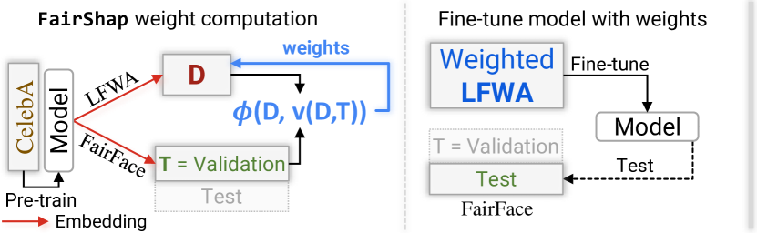
(a) $A=Y$ and $\operatorname{\mathcal{T}}$ is fair.

(b) $A\neq Y$ and $\operatorname{\mathcal{T}}$ is biased.

Figure 2: Pipelines for experiments in Section 5.1 (a) and Section 5.2 (b).

FairShap Re-weighting. In this case, the group fairness metrics are equivalent and thus we report results using $\phi_{i}(\operatorname{{\scriptstyle\text{EOp}}})$: $\phi_{i}(\operatorname{{\scriptstyle\text{EOp}}})$ quantifies the contribution of the $i$th data point (image) in LFWA to the fairness metric (Equal Opportunity) of the model tested on the FairFace dataset.

Baselines. We compare FairShap with three baselines: the pre-trained model using CelebA; the fine-tuned model using LFWA without re-weighting; and a data re-weighting approach using $\bm{\phi(\operatorname{{\scriptstyle\text{Acc}}})}$ from (Ghorbani and Zou, 2019). We report two performance metrics: the accuracy of the models in correctly classifying the sex in the images (Acc) and the Equal Opportunity (EOp), measured as $\operatorname{{\scriptstyle\text{TPR}}}_{M}-\operatorname{{\scriptstyle\text{TPR}}}_{W}$ where $W$ is the disadvantaged group (women in this case). We also report the specific TPR for men and women. A summary of the experimental setup for this scenario is depicted in Figure 2(a).

Results. The results of this experiment are summarized in Table 1. Note how both re-weighting approaches ($\bm{\phi(\operatorname{{\scriptstyle\text{Acc}}})}$ and FairShap) significantly improve the fairness metrics of the models while increasing the accuracy of the model. FairShap yields the best results both in fairness and accuracy. Regarding EOp, the model trained with data re-weighted according to FairShap yields improvements of 88% and 66% when compared to the model trained without re-weighting (LFWA) and the model trained with weights according to $\bm{\phi(\operatorname{{\scriptstyle\text{Acc}}})}$, respectively. In sum, data re-weighting with FairShap is able to leverage complex models trained on biased datasets and improve both their fairness and accuracy.

Training Set	Acc$\uparrow$	TPRW $\mid$ TPRM	EOp $\downarrow$
FairFace	0.909	0.906 $\mid$ 0.913	0.007
CelebA	0.759	0.580 $\mid$ 0.918	0.34
LFWA	0.772	0.635 $\mid$ 0.896	0.26
$\bm{\phi}(\operatorname{{\scriptstyle\text{Acc}}})$	0.793	0.742 $\mid$ 0.839	0.09
FairShap - $\bm{\phi}(\operatorname{{\scriptstyle\text{EOp}}})$	0.799	0.782 $\mid$ 0.813	0.03

Table 1: Performance of the Inception Resnet V1 model tested on the FairFace dataset without and with re-weighting and with protected attribute $A$=$Y$=sex. Best results are highlighted in bold. The arrows next to the metrics’ name indicate if the optimal result of the metric is 0 ($\downarrow$) or 1 ($\uparrow$).

To gain a better understanding of the behavior of FairShap in this scenario, Figure 3 (bottom) depicts a histogram of the $\bm{\phi(\operatorname{{\scriptstyle\text{EOp}}})}$ values on the LFWA training dataset. As seen in the Figure, $\bm{\phi_{i}(\operatorname{{\scriptstyle\text{EOp}}})}$ are mostly positive for the examples labeled as "female" (green) and mostly zero or negative for the examples labeled as "male" (orange). This result makes intuitive sense given that the original model is biased against women, i.e. the probability of misclassification is significantly higher for the images labeled as female than for those labeled as male. Figure 3 (top) depicts the five images with the largest $\phi_{i}(\operatorname{{\scriptstyle\text{EOp}}})$: they all belong to the female category and depict faces with a variety of poses, different facial expressions and from diverse races.

Note how in this case FairShap behaves like a distribution shift method. Figure 4 shows how $\phi_{i}(\operatorname{{\scriptstyle\text{EOp}}})$ shifts the distribution of $\operatorname{\mathcal{D}}$ (LFWA) to be as similar as possible to the distribution of the reference dataset $\operatorname{\mathcal{T}}$ (FairFace). Therefore, biased datasets (such as $\operatorname{\mathcal{D}}$) may be debiased by re-weighting their data according to $\phi_{i}(\operatorname{{\scriptstyle\text{EOp}}})$, yielding models with competitive performance both in terms of accuracy and fairness. Figure 4 illustrates how the group fairness metrics impact individual data points: critical data points are those near the decision boundary. This finding is consistent with recent work that has proposed using Shapley Values to identify counterfactual samples (Albini et al., 2022).

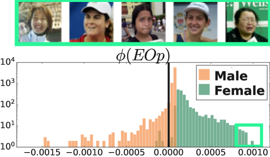
Figure 3: Images with largest $\phi_{i}(\operatorname{{\scriptstyle\text{EOp}}})$ and histogram of $\phi_{i}(\operatorname{{\scriptstyle\text{EOp}}})$ on the LFWA dataset.

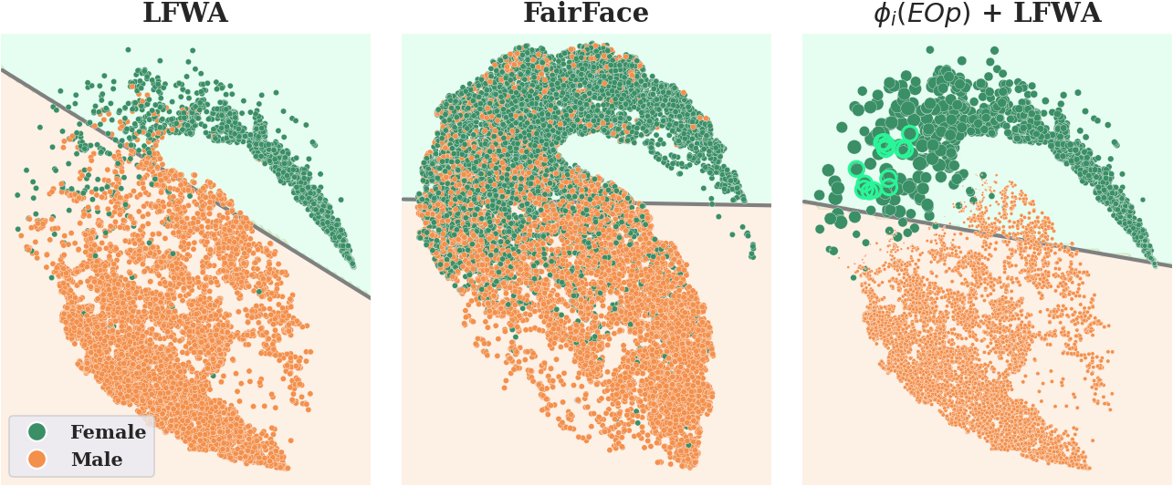
Figure 4: Left: LFWA embeddings. Middle: FairFace embeddings. Right: LFWA embeddings with data point sizes $\propto|\phi_{i}(\operatorname{{\scriptstyle\text{EOp}}})|$. Points with the largest $\phi_{i}(\operatorname{{\scriptstyle\text{EOp}}})$ are highlighted in green. Note how they all correspond to examples of women near the decision boundary of the original LFWA model. As a result of the data-reweighting, the decision boundary has been shifted, yielding a fairer model.

5.2 FairShap when $A\neq Y$ and biased $\operatorname{\mathcal{T}}$

In this section, we consider a common real-life scenario where the target variable $Y$ is not a protected attribute and a single biased dataset $\operatorname{\mathcal{D}}$ is used for training, validation, and testing. Thus, the validation set $\operatorname{\mathcal{T}}$ is obtained from $\operatorname{\mathcal{D}}$ according to the pipeline illustrated in Figure 2(b).

Datasets. We test FairShap on three commonly used datasets in the algorithmic fairness literature: (1) the German Credit (Kamiran and Calders, 2009) dataset (German) with target variable the good or bad individual’s credit risk, and protected groups age and sex; (2) the Adult Income dataset (Kohavi et al., 1996) (Adult) where the task is to predict if the income of a person is more than 50k per year, and sex and race are the protected attributes; and (3) the COMPAS (Angwin et al., 2016) dataset with target variable recidivism and protected attributes sex and race. Section D.6 and Table 7 in the Appendix summarize the statistics of each of these datasets.

Pipeline. The model in all experiments is a Gradient Boosting Classifier (GBC) (Friedman, 2001), known for its competitive performance on tabular data and interpretability properties. The pipeline in this set of experiments is depicted in Figure 2(b). As seen in the Figure, the reference dataset $\operatorname{\mathcal{T}}$ is the validation set of $\operatorname{\mathcal{D}}$. The reported results correspond to the average values of running the experiment 50 times with random splits stratified by sensitive group and label: 70% of the original dataset used for training ($\operatorname{\mathcal{D}}$), 15% for the reference set ($\operatorname{\mathcal{T}}$) and 15% for the test set. Train, reference and test set are stratified by $A$ and $Y$ such that they have the same percentage of $A$ - $Y$ samples as in the original dataset.

FairShap re-weighting. Given that $A\neq Y$, FairShap considers two different fairness-based valuation functions: $\bm{\phi(\operatorname{{\scriptstyle\text{EOp}}})}$ and $\bm{\phi(\operatorname{{\scriptstyle\text{EOdds}}})}$ given by Equation 5 and Equation 6, respectively.

Baselines. To the best of our knowledge, FairShap is the only interpretable, instance-level model-agnostic data reweighting approach for group algorithmic fairness (see Table 4). Thus, we compare its performance with 6 state-of-the-art algorithmic fairness approaches that only partially satisfy FairShap’s properties:

1. Group RW: A group-based re-weighting method that assigns the same weights to all samples from the same category or group according to the protected attribute (Kamiran and Calders, 2012). Thus, this is not an instance-level data re-weighting approach;

2. Post-pro: A post-processing algorithmic fairness method that does not fulfill any of the desiderata, but it is broadly used in the community (Hardt et al., 2016);

3. LabelBias: A model that learns the weights in a in-processing manner and therefore it is neither a pre-processing nor a model-agnostic approach (Jiang and Nachum, 2020);

4. Opt-Pre: A model-agnostic pre-processing approach for algorithmic fairness based on feature and label transformations which does not assign any weights to the data (Calmon et al., 2017);

5. IFs: An Influence Function (IF)-based approach whis is an in-processing a re-training approach, since the weights are computed from the Hessian of a pretrained model. We use the same hyper-parameters reported by the authors for each of the datasets (Li and Liu, 2022); and

6. $\bm{\phi(\operatorname{{\scriptstyle\text{Acc}}})}$: A method based on data re-weighting by means of an accuracy-based valuation function without any fairness considerations (Ghorbani and Zou, 2019).

An extended explanation of the methods and the hyperparameters used can be found in Section D.4.

Experimental setup. We adopt the experimental setup that is commonly followed in the ML community: the weights, the influence functions and the thresholds required by the different methods are computed on the validation set. Furthermore, all the reported results correspond to the mean values of running 50 experiments on each dataset with random stratified train, validation and test set splits in each experiment. Note that some previous works in the algorithmic fairness literature do not perform label-group stratification on the splits, or compute the weights or thresholds using the test set instead of the validation set.

German(S|A)	Accuracy $\uparrow$	M-F1 $\uparrow$	EOp $\downarrow$	EOdds $\downarrow$	Accuracy $\uparrow$	M-F1 $\uparrow$	EOp $\downarrow$	EOdds $\downarrow$
GBC	.697$\pm$.006	.519$\pm$.010	‡.107$\pm$.020	‡.185$\pm$.020	†.704$\pm$.005	.524$\pm$.010	‡.224$\pm$.032	‡.345$\pm$.030
Group RW	.695$\pm$.006	.514$\pm$.010	‡.062$\pm$.019	‡.123$\pm$.025	‡.684$\pm$.004	‡.396$\pm$.041	‡.040$\pm$.025	‡.029$\pm$.026
Postpro	‡.691$\pm$.005	‡.366$\pm$.055	.013$\pm$.014	†.036$\pm$.015	‡.686$\pm$.005	‡.255$\pm$.063	‡.044$\pm$.022	‡.047$\pm$.019
LabelBias	.695$\pm$.006	‡.465$\pm$.035	‡.051$\pm$.019	‡.092$\pm$.026	‡.690$\pm$.004	‡.354$\pm$.053	‡.052$\pm$.029	‡.052$\pm$.035
OptPrep	.694$\pm$.006	.521$\pm$.010	‡.104$\pm$.022	‡.174$\pm$.021	‡.693$\pm$.007	‡.487$\pm$.030	‡.130$\pm$.031	‡.204$\pm$.039
IF	.697$\pm$.006	.519$\pm$.010	‡.107$\pm$.020	‡.185$\pm$.020	†.704$\pm$.005	.524$\pm$.010	‡.224$\pm$.032	‡.345$\pm$.030
$\phi(\operatorname{{\scriptstyle\text{Acc}}})$	.700$\pm$.005	†.507$\pm$.009	‡.097$\pm$.018	‡.184$\pm$.018	.706$\pm$.005	‡.517$\pm$.010	‡.193$\pm$.025	‡.313$\pm$.025
$\bm{\phi(\operatorname{{\scriptstyle\text{EOp}}})}$	‡.683$\pm$.006	‡.460$\pm$.034	.029$\pm$.026	†.049$\pm$.033	‡.685$\pm$.004	‡.373$\pm$.046	.024$\pm$.023	.007$\pm$.021
$\bm{\phi(\operatorname{{\scriptstyle\text{EOdds}}})}$	‡.686$\pm$.006	‡.477$\pm$.009	.002$\pm$.025	.002$\pm$.031	‡.681$\pm$.005	‡.353$\pm$.049	.019$\pm$.020	.003$\pm$.013
Adult(S|R)	Accuracy $\uparrow$	M-F1 $\uparrow$	EOp $\downarrow$	EOdds $\downarrow$	Accuracy $\uparrow$	M-F1 $\uparrow$	EOp $\downarrow$	EOdds $\downarrow$
GBC	.803$\pm$.001	‡.680$\pm$.002	‡.451$\pm$.004	‡.278$\pm$.003	.803$\pm$.001	‡.682$\pm$.002	‡.164$\pm$.010	‡.106$\pm$.006
Group RW	‡.790$\pm$.001	.684$\pm$.002	.002$\pm$.009	.001$\pm$.005	.803$\pm$.001	‡.683$\pm$.002	.010$\pm$.009	.010$\pm$.005
Postpro	‡.791$\pm$.001	†.679$\pm$.004	‡.056$\pm$.013	‡.034$\pm$.007	.802$\pm$.001	.688$\pm$.002	‡.061$\pm$.011	‡.042$\pm$.006
LabelBias	‡.781$\pm$.001	‡.681$\pm$.002	‡.065$\pm$.011	‡.049$\pm$.006	‡.800$\pm$.001	.686$\pm$.002	‡.118$\pm$.013	‡.074$\pm$.007
OptPrep	‡.789$\pm$.001	‡.676$\pm$.004	‡.064$\pm$.029	‡.037$\pm$.017	‡.800$\pm$.001	†.685$\pm$.002	‡.044$\pm$.015	‡.029$\pm$.009
IF	‡.787$\pm$.002	†.681$\pm$.003	‡.159$\pm$.037	‡.092$\pm$.022	‡.797$\pm$.002	†.685$\pm$.002	‡.042$\pm$.020	‡.031$\pm$.012
$\phi(\operatorname{{\scriptstyle\text{Acc}}})$	.804$\pm$.001	‡.681$\pm$.002	‡.452$\pm$.005	‡.279$\pm$.003	.803$\pm$.001	‡.681$\pm$.002	‡.161$\pm$.011	‡.104$\pm$.007
$\bm{\phi(\operatorname{{\scriptstyle\text{EOp}}})}$	‡.790$\pm$.001	.684$\pm$.002	.002$\pm$.009	3e-4$\pm$.005	.802$\pm$.001	‡.683$\pm$.002	.009$\pm$.010	.009$\pm$.005
$\bm{\phi(\operatorname{{\scriptstyle\text{EOdds}}})}$	‡.790$\pm$.001	.683$\pm$.002	8e-4$\pm$.009	.001$\pm$.005	.802$\pm$.001	‡.683$\pm$.002	.007$\pm$.009	.007$\pm$.005
COMPAS(S|R)	Accuracy $\uparrow$	M-F1 $\uparrow$	EOp $\downarrow$	EOdds $\downarrow$	Accuracy $\uparrow$	M-F1 $\uparrow$	EOp $\downarrow$	EOdds $\downarrow$
GBC	.666$\pm$.004	.662$\pm$.004	‡.158$\pm$.014	‡.199$\pm$.014	.663$\pm$.004	.658$\pm$.004	‡.184$\pm$.013	‡.218$\pm$.013
Group RW	.664$\pm$.004	.660$\pm$.004	.020$\pm$.016	‡.038$\pm$.014	‡.649$\pm$.004	‡.646$\pm$.004	‡.028$\pm$.015	.007$\pm$.016
Postpro	‡.660$\pm$.003	‡.655$\pm$.003	.017$\pm$.017	†.030$\pm$.015	‡.647$\pm$.005	‡.642$\pm$.005	1e-4$\pm$.015	‡.026$\pm$.016
LabelBias	‡.639$\pm$.005	‡.612$\pm$.007	.006$\pm$.013	.010$\pm$.014	‡.645$\pm$.004	‡.627$\pm$.005	‡.030$\pm$.011	‡.045$\pm$.014
OptPrep	.664$\pm$.003	.660$\pm$.003	‡.045$\pm$.020	‡.065$\pm$.019	‡.655$\pm$.004	†.651$\pm$.004	‡.044$\pm$.020	‡.078$\pm$.020
IF	.663$\pm$.003	.658$\pm$.003	‡.129$\pm$.016	‡.161$\pm$.015	.660$\pm$.004	.655$\pm$.004	‡.165$\pm$.017	‡.198$\pm$.015
$\phi(\operatorname{{\scriptstyle\text{Acc}}})$	.667$\pm$.004	.662$\pm$.004	‡.156$\pm$.014	‡.198$\pm$.013	.663$\pm$.004	.657$\pm$.004	‡.184$\pm$.013	‡.218$\pm$.013
$\bm{\phi(\operatorname{{\scriptstyle\text{EOp}}})}$	†.661$\pm$.003	†.658$\pm$.004	.013$\pm$.024	.007$\pm$.021	‡.650$\pm$.004	‡.647$\pm$.004	‡.027$\pm$.016	.004$\pm$.017
$\bm{\phi(\operatorname{{\scriptstyle\text{EOdds}}})}$	.663$\pm$.004	.659$\pm$.004	.019$\pm$.021	†.036$\pm$.020	‡.648$\pm$.004	‡.646$\pm$.004	‡.036$\pm$.017	.004$\pm$.018

Table 2: Performance of GBC without and with data re-weighting on benchmark datasets with different sensitive attributes. Best results marked in bold and second-best in italic. Statistically significant differences with the best performing model are denoted by ^‡ for $p<0.01$ and ^† for $p<0.05$.

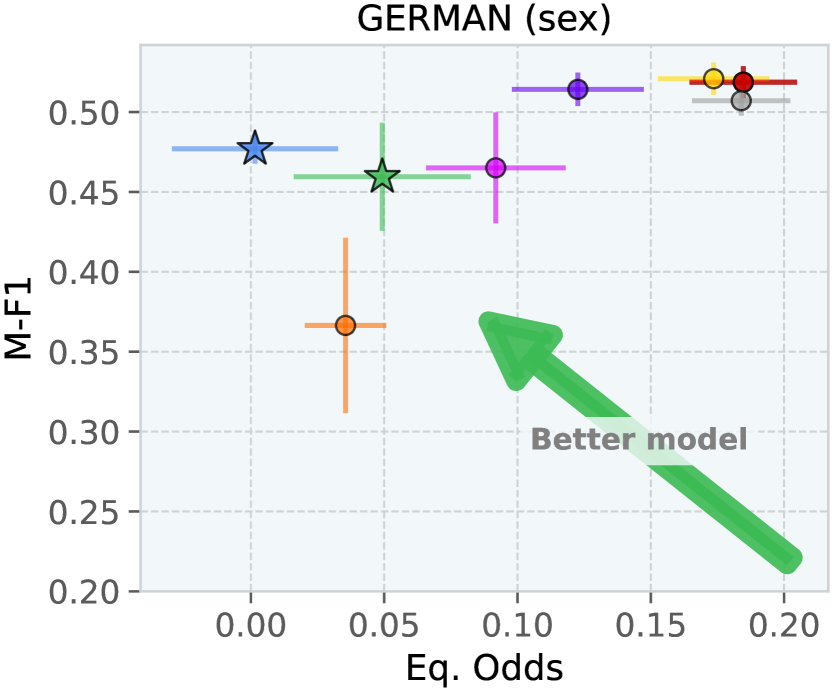
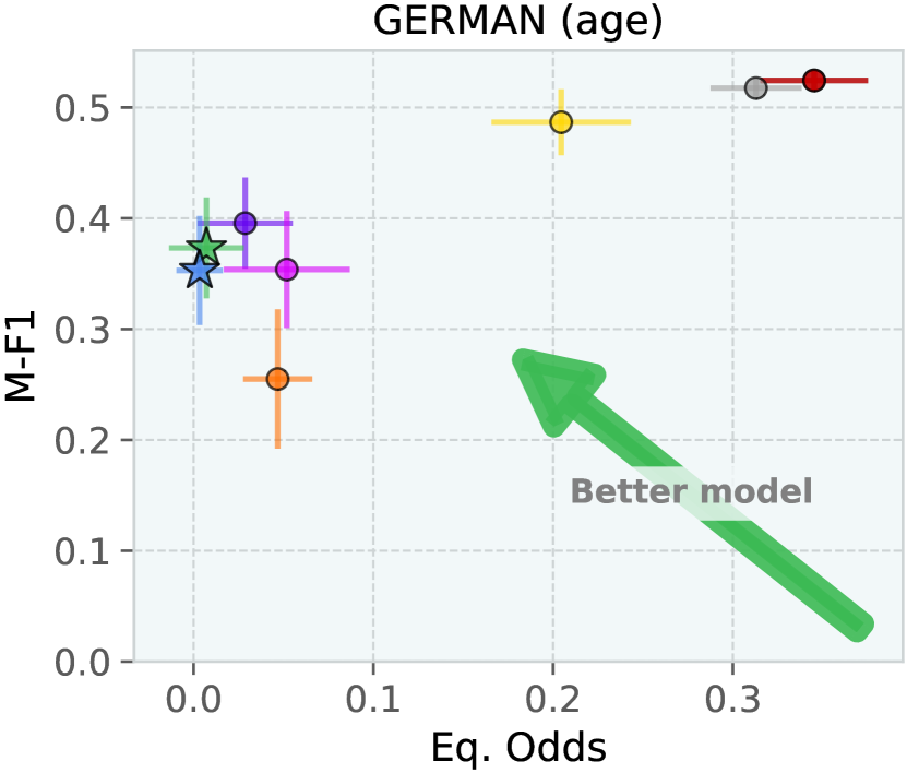
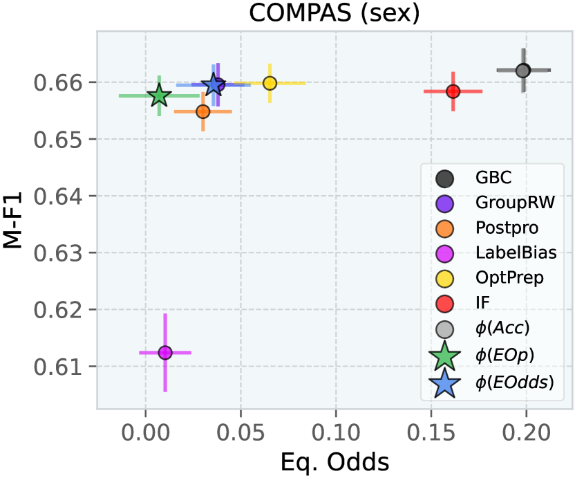
Figure 5: Utility vs fairness analysis. The models trained with data re-weighting via FairShap (depicted as stars in the graphs) improve in fairness while maintaining competitive levels of accuracy when compared to the baselines.

Results. The metrics used for evaluation are accuracy (Acc); Macro-F1 (M-F1), which is an extension of the F1 score that addresses class imbalances, as it is the case in our benchmark datasets (see Section D.5 for a definition of M-F1); equal opportunity (EOp), which is the difference of true acceptance rates; and equalized odds (EOdds), which is the difference between the true and the false positive rates, all of them between groups according to the sensitive attribute. Table 2 summarizes the results, highlighting in bold the best-performing method. The arrows indicate if the optimal result is 0 ($\downarrow$) or 1 ($\uparrow$).

As shown in the Table 2 and Figure 5, data re-weighting with FairShap ($\bm{\phi}(\operatorname{{\scriptstyle\text{EOdds}}})$ and $\bm{\phi}(\operatorname{{\scriptstyle\text{EOp}}})$) generally yields better results in the fairness metrics than the baselines while keeping competitive levels of accuracy. This improvement is notable when compared to the performance of the model built without data re-weighing (GBC). For example, in the German dataset with sex as protected attribute, the model’s Equalized Odds metric is 93x smaller (better) when re-weighting via FairShap ($\bm{\phi}(\operatorname{{\scriptstyle\text{EOdds}}})$) than the baseline model (GBC) and 18x better than the most competitive baseline (PostPro).

From the results, we draw several observations. First, the variance in the accuracy of the post-processing approach (PostPro) is significantly larger than that of other methods. Second, a simple method such as Group RW delivers very competitive results, even better than more sophisticated, recent approaches. Finally, accuracy is not an appropriate metric of the performance of the classifier due to the imbalance of the datasets.

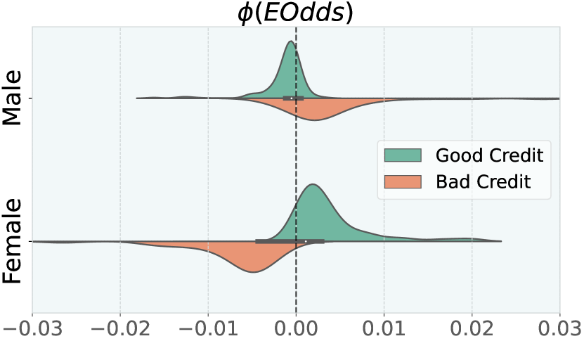
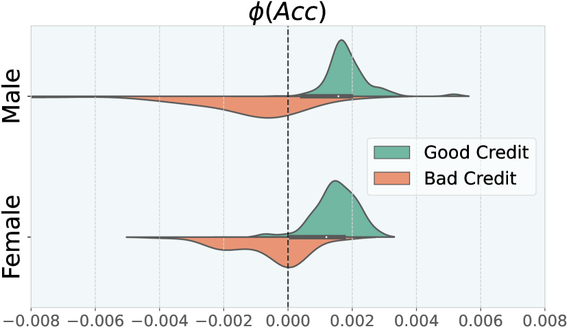
Figure 6: $\phi_{i}(\operatorname{{\scriptstyle\text{EOdds}}})$ (left) and $\phi_{i}(\operatorname{{\scriptstyle\text{Acc}}})$ (right) for the German Credit dataset with $A=\text{sex}$.

To shed further light on the behavior of FairShap, Figure 6 depicts the histograms of the weights according to $\bm{\phi}(\operatorname{{\scriptstyle\text{EOdds}}})$ (left) and $\bm{\phi}(\operatorname{{\scriptstyle\text{Acc}}})$ (right) for the German Credit dataset with sex as protected attribute. Note how the distribution of weights according to $\bm{\phi}(\operatorname{{\scriptstyle\text{Acc}}})$ is similar for males and females, even though the dataset is highly imbalanced: male and female examples with good credit receive larger weights than those with bad credit. Conversely, $\bm{\phi}(\operatorname{{\scriptstyle\text{EOdds}}})$ assigns larger weights to female applicants with good credit than to their male counterparts. In addition, it assigns larger weights to male applicants with bad credit than to their female counterparts. These weight distributions compensate for the imbalances in the raw dataset (both in terms of sex and credit risk), yielding fairer classifiers, as reflected in the results reported in Table 2.

5.3 Accuracy vs Fairness

We are not aware of a theoretical proof that pre-processing model agnostic, data re-weighting methods for algorithmic fairness will always preserve accuracy: the relationship between fairness and accuracy in machine learning models is complex and depends on various factors, including the nature of the dataset and the model used, and the specific fairness metric being optimized.

Shapley Values provide a way to assign weights to individual data points based on their contributions to a particular outcome –such as the model’s prediction or fairness. While Shapley values can be used to re-weight data points to improve fairness according to a specific fairness metric, the impact on accuracy is not guaranteed to be consistent across all datasets and scenarios. However, in many scenarios, particularly when there are a large number of examples in the majority group, optimizing TPR and FPR via data re-weighting does not necessarily lead to a decrease in accuracy for the majority group while improving the model’s fairness for the disadvantaged group. We observe this behavior in all our experiments.

Experiment To further illustrate the impact of FairShap’s data re-weighting on the model’s accuracy and fairness, Figure 7 depicts the utility-fairness curves on the three benchmark datasets (German, Adult and COMPAS). We define a parameter $\alpha$ that controls the contribution to the weights of each data point according to FairShap ($\Phi(\operatorname{{\scriptstyle\text{EOdds}}})$ or $\Phi(\operatorname{{\scriptstyle\text{EOp}}})$), ranging from $\alpha$ = 0 (no data re-weighting) to $\alpha$ = 1 (weights as given by $\Phi(\operatorname{{\scriptstyle\text{EOdds}}})$ or $\Phi(\operatorname{{\scriptstyle\text{EOp}}})$). Thus, the weights of each data point $i$ are computed as $\phi_{i}^{\prime}=(1-\alpha)\mathbf{1}_{|\operatorname{\mathcal{D}}|}+\alpha\phi_{i}$ where $\mathbf{1}_{n}=(1,1,\dotso,1)\in\mathbb{R}^{n}$ is the constant vector and $\phi_{i}$ are the weigths according to FairShap.

As shown in the Figure, the larger the $\alpha$, i.e. the larger the importance of FairShap’s weights, the better the model’s fairness. In some scenarios, such as on the German dataset, we observe a utility-fairness Pareto front where the fairest models correspond to $\alpha$ = 1 and the best performing models correspond to $\alpha$ = 0. Conversely, on the COMPAS (sex) and Adult (race) datasets, larger values of $\alpha$ significantly increase the fairness of the model while keeping similar levels of utility (M-F1 and Accuracy).

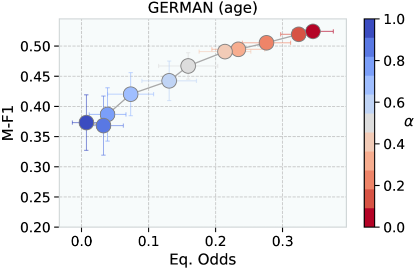
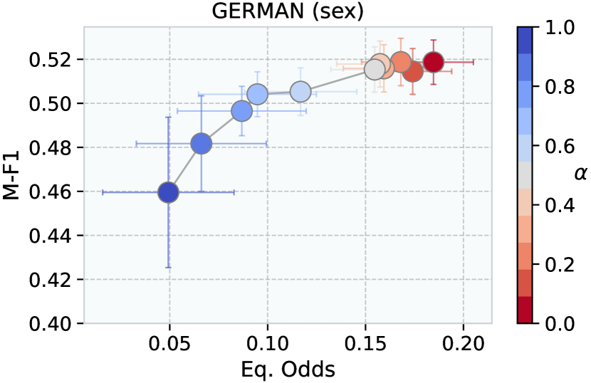
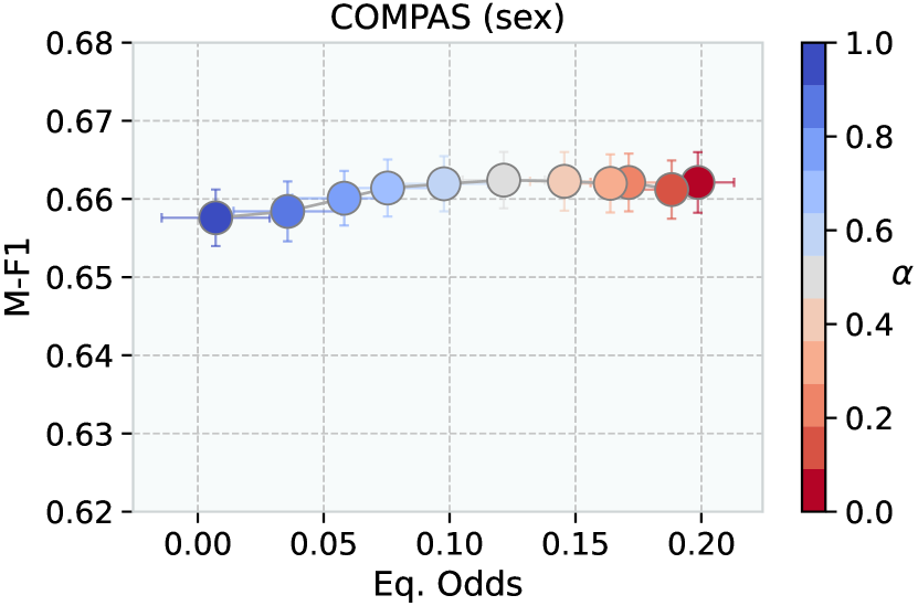
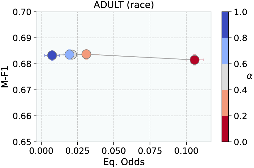
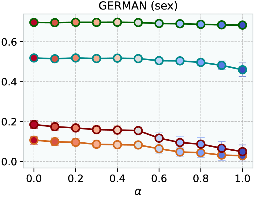
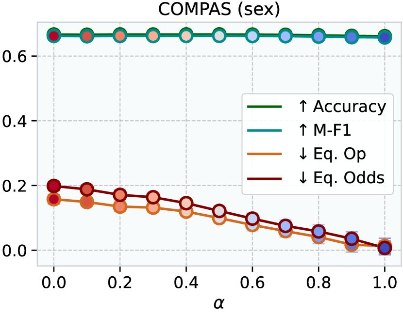
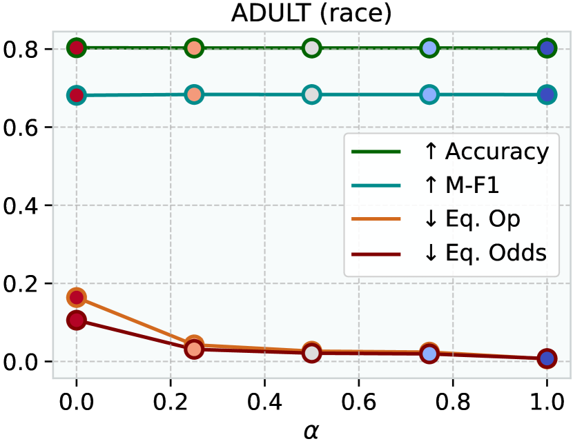
Figure 7: Utility vs fairness trade-off for different values of $\alpha$, where $\alpha=0=$ means no data re-weighting and $\alpha=1$ means data re-weighting according to FairShap’s $\bm{\Phi(\cdot)}$. Results show the mean and 95% CI over 50 random iterations for three different datasets, different utility and fairness metrics and both for $\bm{\Phi(\operatorname{{\scriptstyle\text{EOp}}})}$ and $\bm{\Phi(\operatorname{{\scriptstyle\text{EOdds}}})}$. $\bm{\Phi(\operatorname{{\scriptstyle\text{EOp}}})}$ is used in the German and COMPAS datasets, and $\bm{\Phi(\operatorname{{\scriptstyle\text{EOdds}}})}$ in the Adult dataset. Top graphs show the utility-fairness Pareto front –where utility is given by M-F1 and fairness by EqOdds. The bottom graphs illustrate the Accuracy, M-F1, Equal Opportunity and Equalized Odds for increasing values of $\alpha$.

5.4 Ablation study of the impact of the reference dataset’s size

In this section, we examine the influence of the size of the reference dataset, $T$, and the impact of the alignment between $T$ and the test set on the effectiveness of FairShap’s re-weighting. To do so, we perform an ablation study. We partition the three benchmark datasets (German, Adult and COMPAS) into training (60%, $D$), validation (20%), and testing (20%). We select subsets from the validation dataset –ranging from 5% to 100% of its size– and use them as $T$. For each subset, we compute FairShap’s weights on $D$ with respect to $T$, train a Gradient Boosting Classifier (GBC) model and evaluate its performance on the test set. This process is repeated 10 times with reported results comprising both mean values and standard deviations shown in Figure 8.

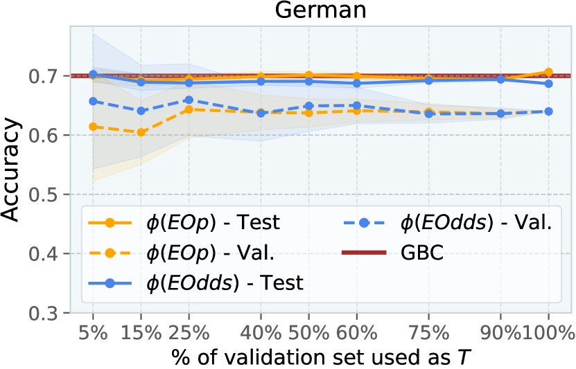
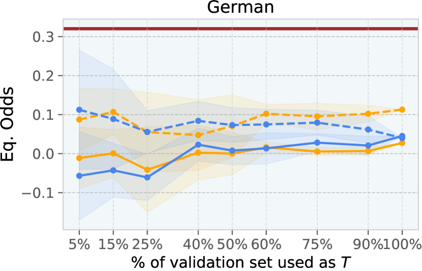
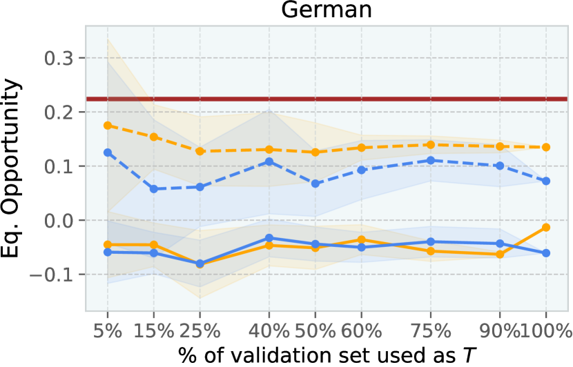
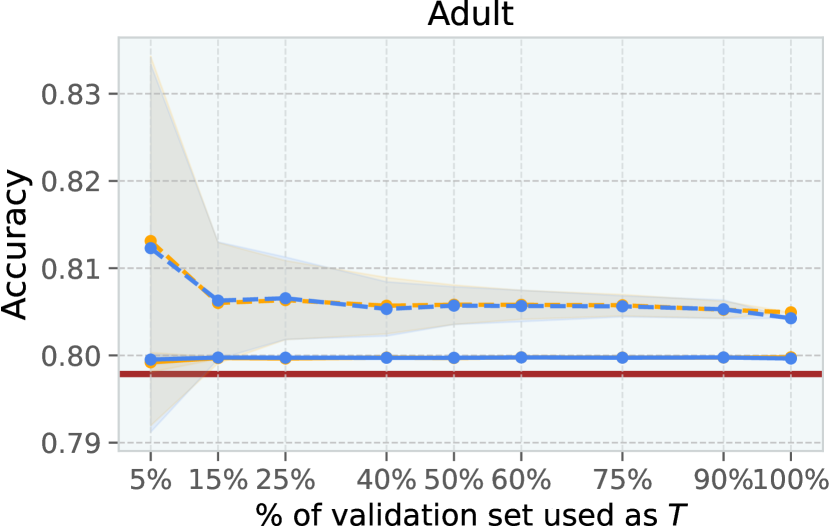
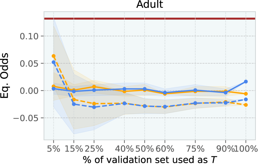
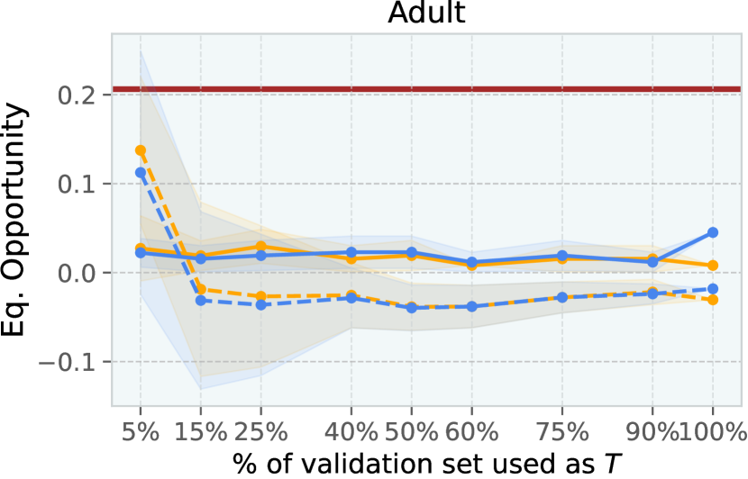
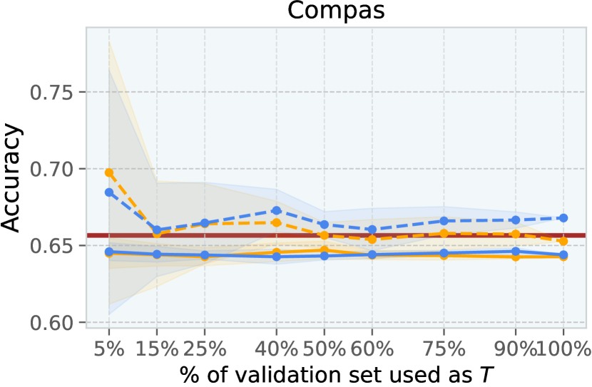
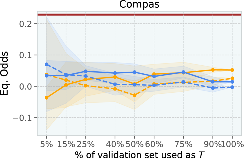
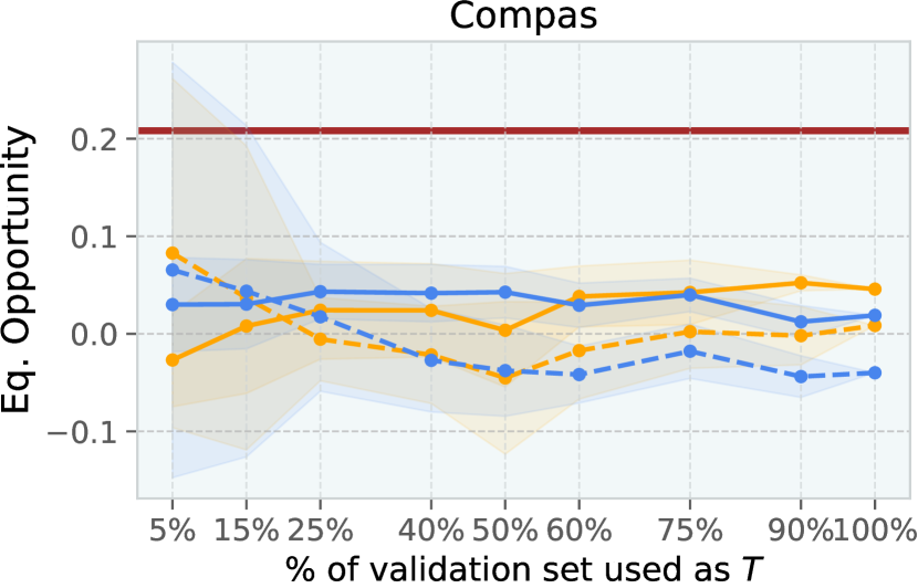
Figure 8: FairShap’s accuracy and fairness metrics ($\phi(\text{EOp})$ and $\phi(\text{EOdds})$) when increasing the size of the validation sets $T$, evaluated on both validation (- -) and test sets (—). The performance of the baseline GBC without re-weighting is shown as a red line. From top to bottom, the rows correspond to the German, Adult and COMPAS datasets, respectively. From left to right, the columns depict the Accuracy, Equalized Odds and Equal Opportunity, respectively.

As shown in the Figures, the size of the validation dataset has a discernible impact on the variance of the evaluation metrics, both in terms of accuracy and fairness. Increasing the size of the reference dataset $T$ leads to a notable reduction in the variability of the outcomes.

5.5 Computational cost

We describe experiments to illustrate FairShap’s computational performance relative to other approaches by applying data re-weighting on synthetic datasets of varying sizes, ranging from 1k to 100k data points, each comprising 200 features. We compare the run time (in seconds) of computing the weights using FairShap, Group Re-weighting (Kamiran and Calders, 2012), OptPrep (Calmon et al., 2017), LabelBias (Jiang and Nachum, 2020) and IFs (Li and Liu, 2022). We leave the post-processing (Hardt et al., 2016) approach out of the comparison since its based on tweaking thresholds after a model is trained, such that the running time heavily depends on the training time of the model of choice. In these experiments, we allocate 80% of the data for training and 20% for validation. With 10 iterations for each configuration, we compute the mean and standard deviation of the run time on an Intel i7-1185G7 3.00GHz CPU. Results are reported in Figure 10.

As seen in the Figure, instance level re-weighting via FairShap is computationally competitive for datasets with up to 30k data points. Group Re-weighting and LabelBias are computationally more efficient than FairShap on datasets with >30k data points.

Note that OptPrep (Calmon et al., 2017) and IFs (Li and Liu, 2022) require a hyperparameter search for each model and each dataset, yielding a significant increase on the computation time. In our experiments, we used the hyperparameters provided by the authors and hence did not have to tune them. Consequently, the actual running time for these methods would significantly increase depending on the number of hyperparameter configurations to be tested. For example, OptPrep consistently requires $\approx 10$ seconds regardless of the dataset’s size. However, a hyperparameter grid-search scenario with 20 different hyperparameter settings and 10-fold cross-validation, would increase the run time to 2,000 seconds (i.e., 10s/it x 20 x 10) or 20,000s for IFs on a dataset size of 60,000 samples (i.e., 100s/it x 20 x 10). These run times are significantly larger than those required to compute FairShap’s weights.

The Figure also depicts FairShap’s execution times (in seconds) with different numbers of features in datasets of increasing sizes. As seen in the Figure, three datasets with 60k, 80k, and 100k instances and feature dimension of 18, have runtimes of 14.7s, 29.1s, and 47.8s.

Finally, we provide an overview of FairShap’s run times for the experiments described in Section 5.2. On the German dataset, FairShap has an average execution time of 0.001s$\pm$0.002, where $|\operatorname{\mathcal{D}}|=700$, $|\operatorname{\mathcal{T}}|=150$, and there are 11 features. In the case of the Adult dataset, the execution time remains consistent at 12.7s$\pm$3, for a dataset with $|\operatorname{\mathcal{D}}|=34189$, $|\operatorname{\mathcal{T}}|=7326$, and 18 features. Finally, for the COMPAS dataset, the execution time is 0.063s$\pm$0.004 on a dataset with $|\operatorname{\mathcal{D}}|=3694$, $|\operatorname{\mathcal{T}}|=792$, and 10 features. These numbers are consistent with the run times reported in Figure 10.

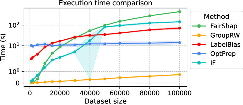
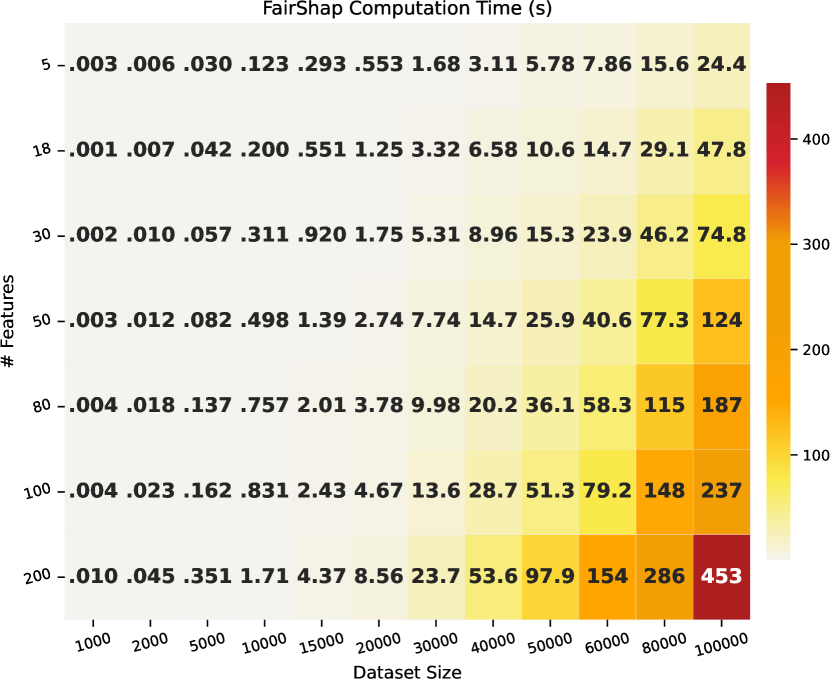
Figure 10: Run time comparison of FairShap’s and baselines with respect to data set size and number of features. Datasets are split in 80% as $D$ and 20% as $T$. We report mean and std run times for 10 iterations. The CPU is an Intel i7-1185G7 3.00GHz.

6 Conclusion, Discussion and Future Work

In this paper, we have proposed FairShap, an instance-level, model-agnostic data re-weighting approach to achieve group fairness via data valuation using Shapley Values. We have empirically validated FairShap with several state-of-the-art datasets in different scenarios and using two different types of models (deep neural networks and GBCs). In our experimental results, the models trained with data re-weighted according to FairShap delivered competitive accuracy and fairness results. Our experiments also highlight the value of using fair reference datasets ($\operatorname{\mathcal{T}}$) for data valuation. We have illustrated the interpretability of FairShap by means of histograms and a latent space visualization. We have also studied the utility vs fairness trade-off, the impact of the size of the reference dataset and FairShap’s computational cost when compared to baseline models. From our experiments, we conclude that data re-weighting by means of FairShap could be a valuable approach to achieve algorithmic fairness. Furthermore, from a practical perspective, FairShap satisfies interpretability desiderata proposed by legal stakeholders and upcoming regulations.

In future work, we plan to assess FairShap’s potential to drive data acquisition and minimization policies, its application to generate counterfactual explanations and its potential to guide data generation processes. We will also explore computationally efficient alternatives like sub-group re-weighting instead of instance-level re-weighting.

Acknowledgments and Disclosure of Funding

This work was supported by the European Commission under Horizon Europe Programme, grant number 101120237 - ELIAS, by Intel corporation, a nominal grant received at the ELLIS Unit Alicante Foundation from the Regional Government of Valencia in Spain (Convenio Singular signed with Generalitat Valenciana, Conselleria de Innovación, Industria, Comercio y Turismo, Dirección General de Innovación) and a grant by the Banc Sabadell Foundation.

Appendix A Preliminaries

A.1 Notation

Symbol	Description
$\operatorname{\mathcal{D}}=\{(x_{i},y_{i})\}^{n}$	Training dataset
$\operatorname{\mathcal{T}}=\{(x_{j},y_{j})\}^{m}$	Reference or background dataset as an external dataset or a partition of $\operatorname{\mathcal{D}}$
$S\subseteq\operatorname{\mathcal{D}}$	Subset of a dataset $\operatorname{\mathcal{D}}$
$A$	Set of variables that are protected attributes.
$\text{TPR}_{A=a}$	True Positive Rate for test points with values in the protected attribute equal to $a$. Also $\operatorname{{\scriptstyle\text{TPR}}}_{a}$ when the protected group is known.
$\phi_{i}(\operatorname{\mathcal{D}},v)$	Shapley Value for data point $i$ in the training dataset $\operatorname{\mathcal{D}}$ according to the performance function $v$
$\bm{\phi}(\operatorname{\mathcal{D}},v)$	Vector with all the SVs of the entire dataset $\in\mathbb{R}^{|\operatorname{\mathcal{D}}|}$.
$v(S,T)$	Value of dataset $S$ w.r.t a reference dataset $\operatorname{\mathcal{T}}$. E.g., the accuracy of a model trained with $S$ tested on $\operatorname{\mathcal{T}}$ ($v=\operatorname{{\scriptstyle\text{Acc}}}$) or the value of Equal Opportunity of of a model trained with $S$ tested on $\operatorname{\mathcal{T}}$ ($v=\text{EOp}$)
$\bm{\Phi}\in\mathbb{R}^{|\operatorname{\mathcal{D}}|\times|\operatorname{\mathcal{T}}|}$	Matrix where $\Phi_{i,j}$ is the contribution of the training point $i\in\operatorname{\mathcal{D}}$ to the correct classification of $j\in\operatorname{\mathcal{T}}$ according to C.2
$\overline{\bm{\Phi}}_{i,:}$	Mean of row $i$
$\overline{\bm{\Phi}}_{i,:|X=x}$	Mean of row $i$ conditioned to columns where $X_{j}=x$
$\mathbf{1}$	Vector of ones := $[1,1,...,1]$

Table 3: Notation.

A.2 Desiderata

Method	D1	D2	D3	D4	D5	D6
	Data Val.	Interpretable	Pre-pro.	Model agnostic	Data RW	Instance-level
FairShap	✓	✓	✓	✓	✓	✓
Group-RW	✗	✓	✓	✓	✓	✗
IFs	✓	✗	✗	✗	✓	✗*
Inpro-RW	✗	✓	✗	✗	✓	✗
Massaging	✗	✓	✓	✓	✗	✗

Table 4: Satisfaction of desiderata by group algorithmic fairness methods similar to FairShap

As previously noted in Section 2, the closest methods to FairShap in the literature are Influence Functions (Wang et al., 2022; Li and Liu, 2022), In-processing reweighting (Krasanakis et al., 2018; Jiang and Nachum, 2020; Chai and Wang, 2022), Group reweighting (Kamiran and Calders, 2012) and Massaging (Feldman et al., 2015; Calmon et al., 2017).

D1 - Data valuation method. Our aim is to propose a novel fairness-aware data valuation approach. Thus, the first desired property concerns whether the method performs data valuation or not (Hammoudeh and Lowd, 2022). Data valuation methods compute the contribution or influence of a given data point to a target function, typically by analyzing the interactions between points (LOO, pair-wise or all the subsets in the data powerset).

D2 - Interpretable. The method should be easy to understand by a broad set of technical and non-technical stakeholders when applied to a variety of scenarios and purposes, including for data minimization, data acquisition policies, data selection for transfer learning, active learning, data sharing, mislabeled example detection and federated learning.

D3 - Pre-processing. The method should provide data insights that can be applicable to train a wide variety of ML learning methods.

D4 - Model agnostic. The computation of model-weights, data valuation values, data insights or data transformations should not rely on learning a model iteratively, to enhance flexibility, computational efficiency, interpretability and mitigate uncertainty. Therefore, this follows the guidelines to make data valuation models data-driven (Sim et al., 2022).

D5 - Data Re-weighting. The data insights drawn from applying the method should be in the form of weights to be applied to the data, which can be used to rebalance the dataset.

D6 - Instance-Level. Different insights or weights are given to each of the data points.

A.3 Clarification of the concept of fairness

Note that the concept of fairness in the definition of the Shapley Values (SVs) is different from algorithmic fairness. The former relates to the desired quality of the SVs to be proportional to how much each data point contributes to the model’s performance. Formally, this translates to the SVs fulfilling certain properties (e.g. efficiency, symmetry, additivity…) to ensure a fair payout. The latter refers to the concept of fairness used in the machine learning literature, as described in the introduction. FairShap uses Shapley Values for data valuation in a pre-processing approach with the objective of mitigating bias in machine learning models. As FairShap is based on the theory of Shapley Values, it also fulfills their four axiomatic properties.

Appendix B Shapley Values proposed in FairShap

FairShap proposes $\bm{\phi(\operatorname{{\scriptstyle\text{EOp}}})}$ and $\bm{\phi(\operatorname{{\scriptstyle\text{EOdds}}})}$ as the data valuation functions to compute the Shapley Values of individual data points in the training set. These functions are computed from the $\bm{\phi(\operatorname{{\scriptstyle\text{TPR}}})},\bm{\phi(\operatorname{{\scriptstyle\text{FPR}}})},\bm{\phi(\operatorname{{\scriptstyle\text{TNR}}})}$ and $\bm{\phi(\operatorname{{\scriptstyle\text{FNR}}})}$ functions, leveraging the Efficiency axiom of the SVs, and the decomposability properties of fairness metrics.

Accuracy (Jia et al. (2019)):

$\phi_{i}(\operatorname{{\scriptstyle\text{Acc}}}):=\frac{1}{|\operatorname{\mathcal{T}}|}\sum_{j\in\operatorname{\mathcal{T}}}\Phi_{i,j}=\overline{\bm{\Phi}}_{i,:}=\mathbb{E}_{j\sim p(\operatorname{\mathcal{T}})}[\Phi_{i,j}]$

True/False Positive/Negative rates (This work):

$\phi_{i}(\operatorname{{\scriptstyle\text{TPR}}}):=\mathbb{E}_{j\sim p(\operatorname{\mathcal{T}}|Y=1)}[\Phi_{i,j}]=\frac{\sum_{j\in\operatorname{\mathcal{T}}}\Phi_{i,j}\mathbb{I}[y_{j}=1]}{|\{x:x\in\operatorname{\mathcal{T}}|y=1\}|}=\overline{\bm{\Phi}}_{i,:|Y=1}$

$\phi_{i}(\operatorname{{\scriptstyle\text{TNR}}}):=\mathbb{E}_{j\sim p(\operatorname{\mathcal{T}}|Y=0)}[\Phi_{i,j}]=\frac{\sum_{j\in\operatorname{\mathcal{T}}}\Phi_{i,j}\mathbb{I}[y_{j}=0]}{|\{x:x\in\operatorname{\mathcal{T}}|y=0\}|}=\overline{\bm{\Phi}}_{i,:|Y=0}$

$\phi_{i}(\operatorname{{\scriptstyle\text{FNR}}}):=\frac{1}{|\operatorname{\mathcal{D}}|}-\phi_{i}(\operatorname{{\scriptstyle\text{TPR}}})$

$\phi_{i}(\operatorname{{\scriptstyle\text{FPR}}}):=\frac{1}{|\operatorname{\mathcal{D}}|}-\phi_{i}(\operatorname{{\scriptstyle\text{TNR}}})$

Conditioned True/False Positive/Negative rates (This work):

$\phi_{i}(\operatorname{{\scriptstyle\text{TPR}}}_{a}):=\mathbb{E}_{j\sim p(\operatorname{\mathcal{T}}|Y=1,A=a)}[\Phi_{i,j}]=\frac{\sum_{j\in\operatorname{\mathcal{T}}}\Phi_{i,j}\mathbb{I}[y_{j}=1,A_{j}=a]}{|\{x:x\in\operatorname{\mathcal{T}}|y=1,A=a\}|}=\overline{\bm{\Phi}}_{i,:|Y=1,A=a}$

$\phi_{i}(\operatorname{{\scriptstyle\text{TPR}}}_{b}):=\mathbb{E}_{j\sim p(\operatorname{\mathcal{T}}|Y=1,A=b)}[\Phi_{i,j}]=\frac{\sum_{j\in\operatorname{\mathcal{T}}}\Phi_{i,j}\mathbb{I}[y_{j}=1,A_{j}=b]}{|\{x:x\in\operatorname{\mathcal{T}}|y=1,A=b\}|}=\overline{\bm{\Phi}}_{i,:|Y=1,A=b}$

$\phi_{i}(\operatorname{{\scriptstyle\text{TNR}}}_{a}):=\mathbb{E}_{j\sim p(\operatorname{\mathcal{T}}|Y=0,A=a)}[\Phi_{i,j}]=\frac{\sum_{j\in\operatorname{\mathcal{T}}}\Phi_{i,j}\mathbb{I}[y_{j}=0,A_{j}=a]}{|\{x:x\in\operatorname{\mathcal{T}}|y=0,A=a\}|}=\overline{\bm{\Phi}}_{i,:|Y=0,A=a}$

$\phi_{i}(\operatorname{{\scriptstyle\text{TNR}}}_{b}):=\mathbb{E}_{j\sim p(\operatorname{\mathcal{T}}|Y=0,A=b)}[\Phi_{i,j}]=\frac{\sum_{j\in\operatorname{\mathcal{T}}}\Phi_{i,j}\mathbb{I}[y_{j}=0,A_{j}=b]}{|\{x:x\in\operatorname{\mathcal{T}}|y=0,A=b\}|}=\overline{\bm{\Phi}}_{i,:|Y=0,A=b}$

$\phi_{i}(\operatorname{{\scriptstyle\text{FPR}}}_{a}):=\frac{1}{|\operatorname{\mathcal{D}}|}-\phi_{i}(\operatorname{{\scriptstyle\text{TNR}}}_{a})$

$\phi_{i}(\operatorname{{\scriptstyle\text{FPR}}}_{b}):=\frac{1}{|\operatorname{\mathcal{D}}|}-\phi_{i}(\operatorname{{\scriptstyle\text{TNR}}}_{b})$

$\phi_{i}(\operatorname{{\scriptstyle\text{FNR}}}_{a}):=\frac{1}{|\operatorname{\mathcal{D}}|}-\phi_{i}(\operatorname{{\scriptstyle\text{TPR}}}_{a})$

$\phi_{i}(\operatorname{{\scriptstyle\text{FNR}}}_{b}):=\frac{1}{|\operatorname{\mathcal{D}}|}-\phi_{i}(\operatorname{{\scriptstyle\text{TPR}}}_{b})$

When A=Y (This work):

$\phi_{i}(\operatorname{{\scriptstyle\text{EOp}}}):=\phi_{i}(\operatorname{{\scriptstyle\text{EOp}}})=\phi_{i}(\operatorname{{\scriptstyle\text{TPR}}})+\phi_{i}(\operatorname{{\scriptstyle\text{TNR}}})-\frac{1}{|\operatorname{\mathcal{D}}|}$

or its bounded version $\phi_{i}(\operatorname{{\scriptstyle\text{EOp}}})=\frac{\phi_{i}(\operatorname{{\scriptstyle\text{TPR}}})+\phi_{i}(\operatorname{{\scriptstyle\text{TNR}}})}{2}$.

See Section C.4 for more details on how to derive these formulas.

When A$\neq$Y (This work):

$\phi_{i}(\operatorname{{\scriptstyle\text{EOp}}}):=\phi_{i}(\operatorname{{\scriptstyle\text{TPR}}}_{a})-\phi_{i}(\operatorname{{\scriptstyle\text{TPR}}}_{b})$

$\phi_{i}(\operatorname{{\scriptstyle\text{EOdds}}}):=\frac{(\phi_{i}(\operatorname{{\scriptstyle\text{FPR}}}_{a})-\phi_{i}(\operatorname{{\scriptstyle\text{FPR}}}_{b}))+(\phi_{i}(\operatorname{{\scriptstyle\text{TPR}}}_{a})-\phi_{i}(\operatorname{{\scriptstyle\text{TPR}}}_{b}))}{2}$

We refer to the reader to Section C.5 for more details on how to obtain these formulas.

Appendix C Methodology

C.1 Algorithmic Fairness Definitions

As aforementioned, the fairness metrics used as valuation functions in FairShap depend on the conditioned true/false negative/positive rates, depending on the protected attribute $A$:

$$\text{TPR}_{A=a} :=\mathbb{P}[\hat{Y}=1|Y=1,A=a],\>\>\text{TNR}_{A=a}:=\mathbb{P}[\hat{Y}=0|Y=0,A=a]$$

$$\text{FPR}_{A=a} :=\mathbb{P}[\hat{Y}=1|Y=0,A=a],\>\>\text{FNR}_{A=a}:=\mathbb{P}[\hat{Y}=0|Y=1,A=a]$$

Note that different fairness metrics are defined by forcing the equality in true/false negative/positive rates between different protected groups. For instance, in a binary classification scenario with a binary sensitive attribute, Equal Opportunity (EOp) and Equalized Odds (EOdds) are defined as follows:

EOp $$:=\mathbb{P}[\hat{y}=1|Y=1,A=a]=\mathbb{P}[\hat{Y}=1|Y=1]$$

EOdds $$:=\mathbb{P}[\hat{y}=1|Y=i,A=a]=\mathbb{P}[\hat{Y}=1|Y=i],\forall i\in\{0,1\}$$

In practical terms, the metrics above are relaxed and computed as the difference for the different groups:

EOp $$:=\text{TPR}_{A=a}-\text{TPR}_{A=b},\>\>\text{EOdds}:=\frac{1}{2}((\operatorname{{\scriptstyle\text{TPR}}}_{A=a}-\operatorname{{\scriptstyle\text{TPR}}}_{A=b})+(\operatorname{{\scriptstyle\text{FPR}}}_{A=a}-\operatorname{{\scriptstyle\text{FPR}}}_{A=b}))$$

The proposed Fair Shapley Values include as their valuation function these group fairness metrics.

C.2 Efficient $k$-NN Shapley Value

Jia et al. (2019) propose an efficient, exact calculation of the Shapley Values by means of a recursive $k$-NN algorithm with complexity $O(N\log N)$. The proposed method yields a matrix $\bm{\Phi}\in\mathbb{R}^{|\operatorname{\mathcal{D}}|\times|\operatorname{\mathcal{T}}|}$ with the contribution of each training point to the accuracy of each test point. Therefore, $\Phi_{i,j}$ defines how much data point $i$ in the training set contributes to the probability of correct classification of data point $j$ in the test set. The intuition behind is that $\Phi_{i,j}$ quantifies to which degree a training point $i$ helps in the correct classification of a test point $j$. The $k$-NN-based recursive calculation is at follows.

For each $j$ in $\operatorname{\mathcal{T}}$:

• Order $i\in\operatorname{\mathcal{D}}$ according to the distance to $j\in\operatorname{\mathcal{T}}\rightarrow(x_{1},x_{2},...,x_{N})$

• Calculate $\Phi_{i,j}$ recursively, starting from the furthest point:

  $$\Phi_{N,j}=\frac{I[y_{x_{N}}=y_{j}]}{N}$$

  $$\Phi_{i,j}=\Phi_{i+1,j}+\frac{I[y_{i}=y_{j}]-I[y_{i+1}=y_{j}]}{\max{K,i}}$$

• $\bm{\Phi}$ is a $|\operatorname{\mathcal{D}}|\times|\operatorname{\mathcal{T}}|$ matrix given by:

  $$\bm{\Phi}=\begin{bmatrix}\Phi_{00}&\cdots&\Phi_{0|\operatorname{\mathcal{T}}|}\\ \vdots&\ddots&\vdots\\ \Phi_{|\operatorname{\mathcal{D}}|0}&\dots&\Phi_{|\operatorname{\mathcal{D}}||\operatorname{\mathcal{T}}|}\\ \end{bmatrix}\in\mathbb{R}^{|\operatorname{\mathcal{D}}|\times|\operatorname{\mathcal{T}}|}$$

where $\Phi_{i,j}$ is the contribution of training point $i$ to the accuracy of the model on test point $j$. Thus, the overall SV of a training point $i$ with respect to the test set is the average of all the values of row $i$ in the SV matrix:

$$\phi_{i}(\operatorname{{\scriptstyle\text{Acc}}})=\frac{1}{m}\sum^{m}_{j=0}\Phi_{i,j}=\overline{\bm{\Phi}}_{i,:}\in\mathbb{R}$$

Note that the mean of a column $j$ in $\bm{\Phi}$ is the accuracy of the model on that test point. The vector with the SV of every training data point is computed as:

$$\bm{\phi}(\operatorname{{\scriptstyle\text{Acc}}})=[\phi_{0},\cdots,\phi_{n}]\in\mathbb{R}^{|\operatorname{\mathcal{D}}|}$$

In addition, given the efficiency axiom of the Shapley Value, the sum of $\bm{\phi}$ is the accuracy of the model on the training set.

$$V(\operatorname{\mathcal{D}})=\sum^{n}_{i=0}\phi_{i}=\sum^{n}_{i=0}\frac{1}{m}\sum^{m}_{j=0}\Phi_{i,j}=\text{Acc}$$

Technically speaking, the process may be parallelized over all test points (columns of the matrix) since the computation is independent, reducing the practical complexity from $O(N\log N)$ to $O(N)$.

C.3 Threshold independence

Computing $\bm{\phi}(\cdot)$ according to the original Shapley Value implementation (Section 3.1) entails evaluating the performance function $v(S)$ on each data point, which requires testing the model trained with $S$. As the group fairness metrics are based on different classification errors, they depend on the classification threshold $\operatorname{\mathcal{T}}$, such that $\text{TP}=|\{\hat{Y}>t|Y=1\}|$, $\text{TN}=|\{\hat{Y}<t|Y=0\}|$, $\text{FP}=|\{\hat{Y}>t|Y=0\}|$ and $\text{FN}=|\{\hat{Y}<t|Y=1\}|$.

However, the previously described efficient method (Section 3.2) is threshold independent since it calculates the accuracy as the average of the probability of correct classification for all test points, as shown in Section C.2.

C.4 FairShap’s weights derivation when $A=Y$

When $A=Y$ in a binary classification task, TPR and TNR are the accuracies for each protected group, respectively. In this case, DP collapses to $\mathbb{P}(\hat{Y}=1|A=a)\rightarrow\mathbb{P}(\hat{Y}=1|Y=a)$ . In this case, EOp measures the similarity of TPRs between groups.

As a result, when $A=Y$ in a binary classification scenario, the group fairness metrics measure the relationship between TPR, TNR, FPR and FNR not conditioned on the protected attribute $A$, since these metrics already depend on $Y$ and $A=Y$. As an example, Equal opportunity is defined in this case as $(\operatorname{{\scriptstyle\text{TPR}}}+\operatorname{{\scriptstyle\text{TNR}}})/2\in[0,1]$ (Hardt et al., 2016):

EOp $$=\frac{\text{TPR}-\text{FPR}+1}{2}=\frac{\text{TPR}-(1-\text{FNR})+1}{2}=\frac{\text{TPR}+\text{TNR}}{2}\in[0,1]$$

Consequently, $\phi_{i}(\operatorname{{\scriptstyle\text{EOp}}})$ $\in[0,1]$ when $A=Y$ can be obtained as follows:

$$\text{EOp}=\frac{\sum_{i\in\operatorname{\mathcal{D}}}\phi_{i}(\operatorname{{\scriptstyle\text{TPR}}})+\sum_{i\in\operatorname{\mathcal{D}}}\phi_{i}(\operatorname{{\scriptstyle\text{TNR}}})}{2}=\sum_{i\in\operatorname{\mathcal{D}}}\frac{\phi_{i}(\operatorname{{\scriptstyle\text{TPR}}})}{2}+\sum_{i\in\operatorname{\mathcal{D}}}\frac{\phi_{i}(\operatorname{{\scriptstyle\text{TNR}}})}{2}$$

$$\phi_{i}(\operatorname{{\scriptstyle\text{EOp}}})=\frac{\phi_{i}(\operatorname{{\scriptstyle\text{TPR}}})+\phi_{i}(\operatorname{{\scriptstyle\text{TNR}}})}{2}$$

C.5 FairShap’s weights derivation when $A\neq Y$

We derive $\bm{\phi}(\operatorname{{\scriptstyle\text{EOp}}})$ and $\bm{\phi}(\operatorname{{\scriptstyle\text{EOdds}}})$ when $A\neq Y$ using the definitions for EOdds and EOp given by:

EOp $$=\operatorname{{\scriptstyle\text{TPR}}}_{A=a}-\operatorname{{\scriptstyle\text{TPR}}}_{A=b}$$

EOdds $$=\frac{1}{2}((\operatorname{{\scriptstyle\text{TPR}}}_{A=a}-\operatorname{{\scriptstyle\text{TPR}}}_{A=b})+(\operatorname{{\scriptstyle\text{FPR}}}_{A=a}-\operatorname{{\scriptstyle\text{FPR}}}_{A=b}))$$

Leveraging the Efficiency property of SVs, $\bm{\phi}(\operatorname{{\scriptstyle\text{EOp}}})$ is computed as:

EOp $$=\sum_{i\in\operatorname{\mathcal{D}}}\phi_{i}(\operatorname{{\scriptstyle\text{TPR}}}_{A=a})-\sum_{i\in\operatorname{\mathcal{D}}}\phi_{i}(\operatorname{{\scriptstyle\text{TPR}}}_{A=b})$$

EOp $$=\sum_{i\in\operatorname{\mathcal{D}}}\left(\phi_{i}(\operatorname{{\scriptstyle\text{TPR}}}_{A=a})-\phi_{i}(\operatorname{{\scriptstyle\text{TPR}}}_{A=b})\right)\rightarrow\phi_{i}(\operatorname{{\scriptstyle\text{EOp}}})=\phi_{i}(\operatorname{{\scriptstyle\text{TPR}}}_{A=a})-\phi_{i}(\operatorname{{\scriptstyle\text{TPR}}}_{A=b})$$

Similarly, $\bm{\phi}(\operatorname{{\scriptstyle\text{EOdds}}})$ can be obtained as follows:

EOdds $$=\frac{1}{2}((\operatorname{{\scriptstyle\text{TPR}}}_{A=a}-\operatorname{{\scriptstyle\text{TPR}}}_{A=b})+(\operatorname{{\scriptstyle\text{FPR}}}_{A=a}-\operatorname{{\scriptstyle\text{FPR}}}_{A=b}))$$

$$=\frac{(\sum_{i\in\operatorname{\mathcal{D}}}\phi_{i}(\operatorname{{\scriptstyle\text{TPR}}}_{A=a})-\sum_{i\in\operatorname{\mathcal{D}}}\phi_{i}(\operatorname{{\scriptstyle\text{TPR}}}_{A=b}))+(\sum_{i\in\operatorname{\mathcal{D}}}\phi_{i}(\operatorname{{\scriptstyle\text{FPR}}}_{A=a})-\sum_{i\in\operatorname{\mathcal{D}}}\phi_{i}(\operatorname{{\scriptstyle\text{FPR}}}_{A=b}))}{2}$$

$$=\frac{\sum_{i\in\operatorname{\mathcal{D}}}\left(\phi_{i}(\operatorname{{\scriptstyle\text{TPR}}}_{A=a})-\phi_{i}(\operatorname{{\scriptstyle\text{TPR}}}_{A=b})\right)+\sum_{i\in\operatorname{\mathcal{D}}}\left(\phi_{i}(\operatorname{{\scriptstyle\text{FPR}}}_{A=a})-\sum_{i\in\operatorname{\mathcal{D}}}\phi_{i}(\operatorname{{\scriptstyle\text{FPR}}}_{A=b})\right)}{2}$$

$$=\frac{\sum_{i\in\operatorname{\mathcal{D}}}\left(\left(\phi_{i}(\operatorname{{\scriptstyle\text{TPR}}}_{A=a})-\phi_{i}(\operatorname{{\scriptstyle\text{TPR}}}_{A=b})\right)+\left(\phi_{i}(\operatorname{{\scriptstyle\text{FPR}}}_{A=a})-\phi_{i}(\operatorname{{\scriptstyle\text{FPR}}}_{A=b})\right)\right)}{2}\rightarrow$$

$$\rightarrow\phi_{i}(\operatorname{{\scriptstyle\text{EOdds}}}) =\frac{\left(\phi_{i}(\operatorname{{\scriptstyle\text{TPR}}}_{A=a})-\phi_{i}(\operatorname{{\scriptstyle\text{TPR}}}_{A=b})\right)+\left(\phi_{i}(\operatorname{{\scriptstyle\text{FPR}}}_{A=a})-\phi_{i}(\operatorname{{\scriptstyle\text{FPR}}}_{A=b})\right)}{2}$$

C.6 Extension to multi-label and categorical sensitive attribute scenarios

As in the binary setting, the group fairness metrics are computed from TPR, TNR, FPR and FNR. Taking as an example TPR, the main change consists of replacing $y=1$ or $y=0$ for $y_{j}$=y:

$$\phi_{i}(\operatorname{{\scriptstyle\text{TPR}}}_{\mid Y=y})=\mathbb{E}_{j\sim p(\operatorname{\mathcal{T}}\mid Y=y)}[\Phi_{i,j}]=\frac{\sum_{j\in\operatorname{\mathcal{T}}}\Phi_{i,j}\mathbb{I}[y_{j}=y]}{|\{x:x\in\operatorname{\mathcal{T}}|y=y\}|}=\overline{\bm{\Phi}}_{i,:|Y=y}$$

The conditioned version $\phi_{i}(\operatorname{{\scriptstyle\text{TPR}}}_{a})$ may be obtained as:

$$\phi_{i}(\operatorname{{\scriptstyle\text{TPR}}}_{\mid Y=y,A=a})=\mathbb{E}_{j\sim p(\operatorname{\mathcal{T}}\mid Y=y,A=a)}[\Phi_{i,j}]=\frac{\sum_{j\in\operatorname{\mathcal{T}}}\Phi_{i,j}\mathbb{I}[y_{j}=y,A_{j}=a]}{|\{x:x\in\operatorname{\mathcal{T}}|y=y,A=a\}|}=\overline{\bm{\Phi}}_{i,:|Y=y,A=a}$$

where $y$ and $a$ can be categorical variables. In the scenario where $a$ is not a binary protected attribute, EOp is calculated as $\text{EOp}_{a}=|\text{TPR}-\text{TPR}_{A=a}|\>\forall a\in A$ , and then the maximum difference is selected as the unique EOp for the model $\text{EOp}=\max_{\forall a\in A}\text{EOp}_{a}$, i.e. the EOp for the group that most differs from the TPR of the entire dataset. Therefore, $\phi_{i}(\operatorname{{\scriptstyle\text{EOp}}})$ for each data point is computed as $\phi_{i}(\operatorname{{\scriptstyle\text{EOp}}})=\phi_{i}(\operatorname{{\scriptstyle\text{TPR}}}_{a})-\phi_{i}(\operatorname{{\scriptstyle\text{TPR}}})$ being $a$ the protected attribute with maximum EOp. The same procedure applies to EOdds. In other words, $\phi_{i}(\operatorname{{\scriptstyle\text{EOp}}})=\mathbb{E}_{j\sim p(\operatorname{\mathcal{T}}\mid Y=y,A=a)}[\Phi_{i,j}]-\mathbb{E}_{j\sim p(\operatorname{\mathcal{T}}\mid Y=y)}[\Phi_{i,j}]$.

Appendix D Experiments

The code for all the experiments described in this paper is publicly available at https://anonymous.4open.science/r/fair-shap.

D.1 Impact of biased datasets on the models’ evaluation

It is crucial to be aware that models trained on biased datasets may perform well in terms of accuracy and fairness when tested against themselves. However, when evaluated against fair datasets, their performance can deteriorate significantly. It is widely recognized that biased datasets can lead to biased machine learning models, which can perpetuate and exacerbate societal inequities. These models can reinforce existing biases and stereotypes, leading to unfair and discriminatory outcomes for certain groups, especially underrepresented or marginalized communities. Therefore, it is essential to develop fair reference datasets to ensure that machine learning models are tested in a way that accounts for the potential impact of bias and promotes fairness. In light of this, we present here the results of our experiments that illustrate the performance and fairness of a model trained and tested on three different dataset combinations: large yet biased datasets (LFWA and CelebA) and a smaller and unbiased dataset (FairFace). As illustrated in Table 5, the performance of the models trained on biased datasets (LFWA and CelebA) and tested on fair datasets (FairFace) is significantly worse than when tested on the biased datasets.

Train \ Test	FairFace	LFWA	CelebA
FairFace	90.9 $|$ 0.01	95.7 $|$ 0.03	96.7 $|$ 0.09
LFWA	77.2 $|$ 0.49	96.6 $|$ 0.08	98.3 $|$ 0.02
CelebA	76.1 $|$ 0.61	96.9 $|$ 0.09	98.2 $|$ 0.01

Table 5: Sex classification results reported as Acc $\uparrow|$ AccDisp $\downarrow$ for an Inception Resnet V1 model trained and tested on different datasets. The protected attribute $A$ is sex. Note the degradation in performance when training on a biased dataset and evaluating on a fair dataset (marked in red font in the Table).

D.2 Experiments on synthetic datasets

$\phi(\operatorname{{\scriptstyle\text{TPR}}})$ and $\phi(\operatorname{{\scriptstyle\text{TNR}}})$

In this section, we present a visual analysis of $\phi(\operatorname{{\scriptstyle\text{TPR}}})$ and $\phi(\operatorname{{\scriptstyle\text{TPR}}})$ using a synthetic binary classification dataset featuring two Gaussian distributions.

Figure 11 illustrates the extent to which each data point contributes positively or negatively to the True Positive Rate (TPR) and True Negative Rate (TNR). Points with larger $\phi(\operatorname{{\scriptstyle\text{TPR}}})$ correspond to instances from the positive class located on the correct side near the decision boundary whereas points with smaller $\phi(\operatorname{{\scriptstyle\text{TPR}}})$ represent positive class points placed on the wrong side of the decision boundary. The same logic applies to $\phi(\operatorname{{\scriptstyle\text{TNR}}})$ with respect to the negative class points, providing intuitive insights related to the contributions to TPR or TNR of different data points.

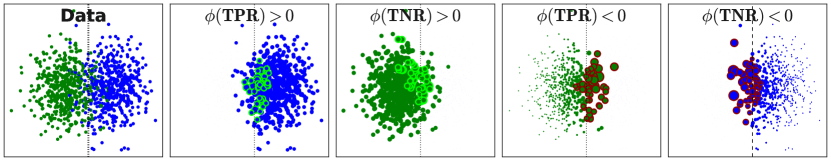
Figure 11: Synthetic example with positive (blue) and negative (green) classes. Data points with the 50 largest (in green) and smallest (in red) $\phi_{i}$ are highlighted. Size $\propto|\phi_{i}|$, i.e. larger when grater in $\phi_{i}(\cdot)>0$ and larger when smaller in $\phi_{i}(\cdot)<0$. Points belonging to the positive and negative class are colored as blue and green, respectively.

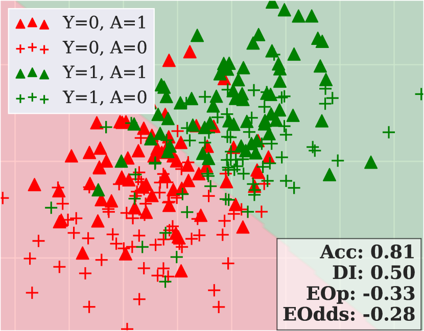
(a) Original Data

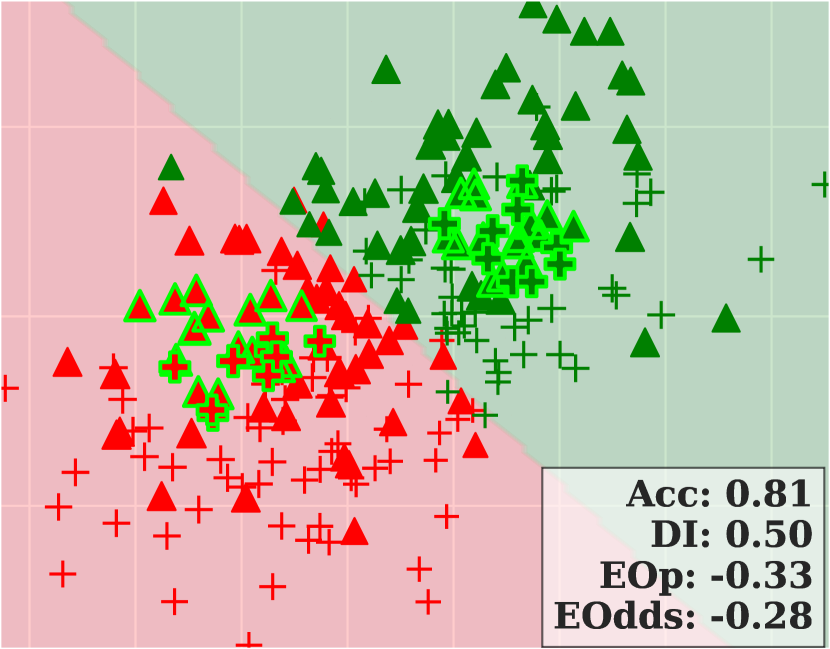
(b) $\phi(\operatorname{{\scriptstyle\text{Acc}}})$

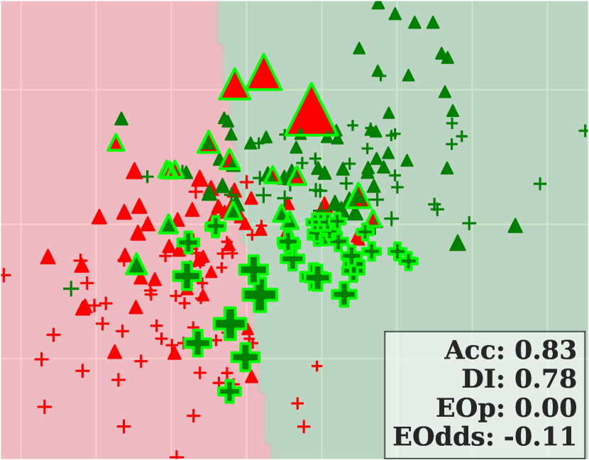
(c) $\phi(\operatorname{{\scriptstyle\text{EOp}}})$

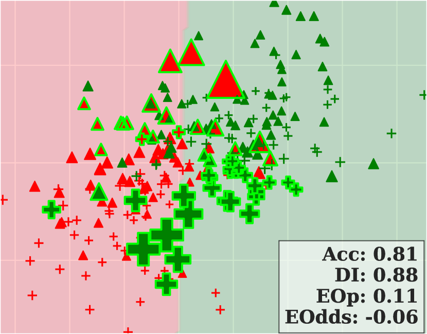
(d) $\phi(\operatorname{{\scriptstyle\text{EOdds}}})$

Figure 12: Synthetic example where the group FPR and the group FNR differences have different signs (Case I in Zafar et al. (2017)). The size of each data point is proportional to its $\mathbf{|\phi}(\cdot)|$. The top-50 points, according to each $\mathbf{\phi}(\cdot)$, are highlighted in green. The label $Y=1$ corresponds to the favorable outcome (colored in green), and the privileged group is defined by $A=1$ (represented as triangles ▲). The label $Y=0$ corresponds to the unfavorable outcome (colored in red), and the disadvantaged group is defined by $A=0$ (represented as crosses ✛). Logistic Regression models are trained on different re-weighted versions of the data and evaluated using the same test split. Decision regions are shaded.

A$\neq$Y

In this scenario, we generate synthetic data where the protected attribute $A$ and the label $Y$ are slightly correlated. Specifically, we employ Case I from Zafar et al. (2017) as a reference, where the disparity between the False Negative Rate (FNR) and the False Positive Rate (FPR) exhibits a distinct sign: larger FPR for the privileged group and larger FNR for the disadvantaged group. Consequently, the mean overlap occurs between the unfavorable-privileged and the favorable-disadvantaged classes.

Figure 12 visualizes data instances of this scenario as points, where the size of each point is proportional to its $\mathbf{|\phi}(\cdot)|$. Additionally, we highlight in green the top-50 points based on their $\mathbf{\phi}(\cdot)$. The label $Y=1$ corresponds to the favorable outcome (colored in green), and the privileged group is defined by $A=1$ (represented as triangles). The label $Y=0$ corresponds to the unfavorable outcome (colored in red), and the disadvantaged group is defined by $A=0$ (represented as crosses). We train unconstrained Logistic Regression models on various versions of the data and assess their performance using the same test split.

The experimental results shown in Figure 12 illustrate significant changes in the decision boundaries of the models when trained using weights given by $\phi(\operatorname{{\scriptstyle\text{EOp}}})$ or $\phi(\operatorname{{\scriptstyle\text{EOdds}}})$, yielding fairer models while maintaining comparable or improved levels of accuracy. Moreover, the analysis reveals that both $\phi(\operatorname{{\scriptstyle\text{EOp}}})$ and $\phi(\operatorname{{\scriptstyle\text{EOdds}}})$ predominantly prioritize instances in the unfavorable-privileged (red triangles) and favorable-disadvantaged groups (green crosses).

D.3 Computer vision training set-up

In the experiment described in Section 5, the Inception Resnet V1 model was initially pre-trained on the CelebA dataset and subsequently fine-tuned on LFWA. Binary cross-entropy loss and the Adam optimizer were used in both training phases. The learning rate was set to 0.001 for pre-training and reduced to 0.0005 for fine-tuning, each lasting 100 epochs. Training batches consisted of 128 images with an input shape of (160x160), and a patience parameter of 30 was employed for early stopping, saving the model with the highest accuracy on the validation set. The classification threshold for this model was set at 0.5.

D.4 Description of the baselines used in the experiments (Section 5.2)

Group RW (Kamiran and Calders, 2012)]: A group-based re-weighting method that assigns the same weights to all samples from the same category or group according to the protected attribute. Weights are assigned to compensate that the expected probability if $A$ and $Y$ where independent on $\operatorname{\mathcal{D}}$ is higher than the observed probability value.

$$w_{i}(a_{i},y_{i})=\frac{|\{X\in\operatorname{\mathcal{D}}|X(A)=a_{i}\}|\times|\{X\in\operatorname{\mathcal{D}}|X(Y)=y_{i}\}|}{|\{\operatorname{\mathcal{D}}\}|\times|\{X\in\operatorname{\mathcal{D}}|X(A)=a_{i},X(Y)=y_{i}\}|}$$

Group RW does not require any additional parameters for its application. We use the implementation from AIF360 (Bellamy et al., 2019).

Post-pro (Hardt et al., 2016): A post-processing algorithmic fairness method that assigns different classification thresholds for different groups to equalize error rates. The method applies a threshold to the predicted scores to achieve this balance.

In our experiments, we adopt an enhanced implementation of this method, provided by the authors and based on the error-parity library. This implementation makes its predictions using an ensemble of randomized classifiers instead of relying on a deterministic binary classifier. A randomized classifier is one that lies within the convex hull of the classifier’s ROC curve at a specific target ROC point. This approach enhances the method’s ability to satisfy the equality of error rates.

LabelBias (Jiang and Nachum, 2020): This model learns the weights in an iterative, in-processing manner based on the model’s error. Consequently, this method is neither a pre-processing nor a model-agnostic approach.

We use an implementation based on the google-research/label_bias repository, which is the official implementation of the original work. We apply the settings described in Jiang and Nachum (2020) and use a learning rate of $\mu=1$ with a fixed number of 100 iterations.

Opt-Pre (Calmon et al., 2017): A model-agnostic pre-processing approach for algorithmic fairness based on feature and label transformations solving a a convex optimization.

We use the pre-defined hyperparameters provided by both the authors (see Calmon et al., 2017, Supplementary 4.1-4.3) and the AIF360 library: the discrimination parameter $\epsilon=0.05$; distortion constraints of [0.99, 1.99, 2.99], which are distance thresholds for individual distortions; and finally we use probability bounds of [.1, 0.05, 0] for each threshold in the distortion constraints (Calmon et al., 2017, Eq. 5). We use the implementation from AIF360 (Bellamy et al., 2019).

IFs (Li and Liu, 2022): An Influence Function (IF)-based approach, where the influence of each training sample is modeled with regard to a fairness-related quantity and predictive utility. This is an in-processing, and re-training approach, as follows. First, a model is trained. Second, the Hessian vector product is computed for every sample $\mathbf{H}^{-1}_{\hat{\theta}(\mathbf{1})}\nabla^{2}_{\theta}\ell(x_{i};\hat{\theta}(\mathbf{1})$, where the Hessian is defined as $\mathbf{H}_{\hat{\theta}(\mathbf{1})}=\sum_{i=1}\nabla^{2}_{\theta}\ell(x_{i};\hat{\theta}(\mathbf{1}))$ and $\hat{\theta}(\mathbf{1})$ is the empirical risk minimization with equal sample weights. Third, the influence functions for every sample are obtained based on the vector products. Fourth, a linear problem based on these influence functions is solved to compute the weights. Finally, the model is re-trained with the new weights. Notably, this method exhibits behavior resembling hard removal re-weighing –as observed in our experiments– where the weights are either 0 or 1 for all samples, with no in-between values. This pattern aligns with the observations made by the authors themselves. While the method is theoretically categorized as individual re-weighting, in practice, it works as a sampling method.

We set the hyperparameters to the values reported by the authors for each dataset. Namely, for the German dataset: $\alpha=1$, $\beta=0$, $\gamma=0$ and $\mathrm{l2reg}=5.85$. For the Adult dataset: $\alpha=1$, $\beta=0.5$, $\gamma=0.2$ and $\mathrm{l2reg}=2.25$. Finally, for the COMPAS dataset: $\alpha=1$, $\beta=0.2$, $\gamma=0.1$ and $\mathrm{l2reg}=37$. We use an implementation from the influence-fairness repository by Brandeis ML, which needs the request and installation of a Gurobi license.

$\bm{\phi(\operatorname{{\scriptstyle\text{Acc}}})}$ (Ghorbani and Zou, 2019): A method based on data re-weighting by means of an accuracy-based data valuation function without any fairness considerations. This method is explained in detail on Sections 3.2 and C.2. We use our own efficient implementation using the Numba python library.

D.5 Utility metrics

The reported experiments with the tabular datasets (i.e. German, Adult and COMPAS) include different utility metrics to evaluate the performance of the models.

In imbalanced datasets, where one class significantly outweighs the other in terms of the number of examples, accuracy does not provide a comprehensive assessment of a model’s performance, given that high accuracies might be obtained by a simple model that predicts the majority class. In these cases, the F1 metric is more appropiate, defined as $2\times\frac{\text{precision}\times\text{recall}}{\text{precision}+\text{recall}}$, since it considers both precision ($\frac{\text{TP}}{\text{TP}+\text{FP}}$) and recall ($\text{TPR}=\frac{\text{TP}}{\text{TP}+\text{FN}}$).

However, the F1 metric is only meaningful when the positive class is the minority class. Otherwise, i.e. if the positive class is the majority class, a constant classifier that always predicts the positive class can achieve a high F1 values. For example, in a scenario where the positive class has 100 examples and the negative class only 20, a simple model that always predicts the positive class will get an accuracy of 0.83 and a F1 score of 0.91. However, the F1 score for the negative class would be 0 in this case.

The Macro-F1 metric arises as a solution to this scenario. Unlike the standard F1 score, the Macro-F1 computes the average of the F1 scores for each class. Thus, the Macro-F1 score can provide insight into the model’s performance on every class for imbalanced datasets.

Thus, in our experiments with tabular data, we report the Macro-F1 scores.

D.6 Dataset statistics

Image Datasets Total number of images and male/female distribution from the CelebA, LFWA and FairFace datasets are shown on Table 6.

Dataset	Train	Validation	Test
CelebA	94509$|$68261	11409$|$8458	12247$|$7715
LFWA	7439$|$2086	2832$|$876	–
FairFace	45986$|$40758	9197$|$8152	5792$|$5162

Table 6: Face Datasets Statistics. Rows stand for #male$|$#female.

Fairness Benchmark Datasets The tables below summarize the statistics of the German, Adult and COMPAS datasets in terms of the distribution of labels and protected groups. Note that all the nomenclature regarding the protected attribute names and values is borrowed from the official documentation of the datasets.

Table 7(a) shows the distributions of sex and label for the German dataset (Kamiran and Calders, 2009). It contains 1,000 examples with target binary variable the individual’s credit risk and protected groups age and sex. We use ‘Good Credit’ as the favorable label (1) and ‘Bad Credit‘ as the unfavorable one (0). Regarding age as a protected attribute, ‘Age>25’ and ’Age<25’ are considered the favorable and unfavorable groups, respectively. When using sex as protected attribute, ‘male’ and ’female’ are considered the privileged and unprivileged groups, respectively. Features used are the one-hot encoded credit history (delay, paid, other), one-hot encoded savings (>500, <500, unknown) and one-hot encoded years of employment (1-4y, >4y, unemployed).

A\Y	Bad	Good	Total
Male	191	499	690 (69%)
Female	109	201	310 (31%)
Age$>$25	220	590	810 (81%)
Age$<$25	80	110	190 (19%)
Total	300 (30%)	700 (70%)	1,000

(a) German Credit

A\Y	$<$50k	$>$50k	Total
White	31,155	10,607	41,762 (86%)
non-White	6,000	1,080	7,080 (14%)
Male	22,732	9,918	32,650 (67%)
Female	14,423	1,769	16,192 (33%)
Total	37,155 (76%)	11,687 (24%)	48,842

(b) Adult Income

A\Y	Recid	No Recid	Total
Male	2,110	2,137	4,247 (80%)
Female	373	658	1,031 (20%)
Caucasian	822	1,281	2,103 (40%)
non-Cauc.	1,661	1,514	3,175 (60%)
Total	2,483 (47%)	2,795 (53%)	5,278

(c) COMPAS

Table 7: Tabular datasets statistics.

Table 7(b) depicts the data statistics for the Adult Income dataset (Kohavi et al., 1996). This dataset contains 48,842 examples where the task is to predict if the income of a person is more than 50k per year, being >50k considered as the favorable label (1) and <50k as the unfavorable label (0). The protected attributes are race and sex. When race is the protected attribute, ‘white’ refers to the privileged group and ‘non-white’ to the unprivileged group. With sex as protected attribute, ‘Male’ is considered the privileged group and ‘female’ the unprivileged group. The features are the one-hot encoded age decade (10, 20, 30, 40, 50, 60, >70) and education years (<6, 6, 7, 8, 9, 10, 11, 12, >12).

Table 7(c) contains the statistics about the COMPAS (Angwin et al., 2016) dataset. This dataset has 5,278 examples with target binary variable recidivism. We use ‘Did recid’ as the unfavorable label (0) and ‘No recid’ as the favorable label (1). When sex is the protected attribute, ‘male’ is the unprivileged group and ‘female’ as the privileged one. When using race as protected attribute, ‘caucasian’ is the privileged group and ‘non-caucasian’ the unprivileged one. Regarding the features, we use one-hot encoded age (<25, 25-45, >45), one-hot prior criminal records of defendants (0, 1-3, >3) and one-hot encoded charge degree of defendants (Felony or Misdemeanor).

All datasets are pre-processed using AIF360 by Bellamy et al. (2019), which use the same pre-processing as in Calmon et al. (2017).

References

- Albini et al. (2022) E. Albini, J. Long, D. Dervovic, and D. Magazzeni. Counterfactual shapley additive explanations. In 2022 ACM Conference on Fairness, Accountability, and Transparency, pages 1054–1070, 2022.
- Ali et al. (2021) J. Ali, P. Lahoti, and K. P. Gummadi. Accounting for model uncertainty in algorithmic discrimination. In Proceedings of the 2021 AAAI/ACM Conference on AI, Ethics, and Society, pages 336–345, 2021.
- Angwin et al. (2016) J. Angwin, J. Larson, S. Mattu, and L. Kirchner. Machine bias: There’s software used across the country to predict future criminals. and it’s biased against blacks. propublica, may 23, 2016.
- Barocas and Selbst (2016) S. Barocas and A. D. Selbst. Big data’s disparate impact. California law review, pages 671–732, 2016.
- Barocas et al. (2019) S. Barocas, M. Hardt, and A. Narayanan. Fairness and Machine Learning: Limitations and Opportunities. The MIT Press, 2019.
- Basu et al. (2021) S. Basu, P. Pope, and S. Feizi. Influence functions in deep learning are fragile. In International Conference on Learning Representations, 2021.
- Bellamy et al. (2019) R. K. Bellamy, K. Dey, M. Hind, S. C. Hoffman, S. Houde, K. Kannan, P. Lohia, J. Martino, S. Mehta, A. Mojsilović, et al. Ai fairness 360: An extensible toolkit for detecting and mitigating algorithmic bias. IBM Journal of Research and Development, 63(4/5):4–1, 2019.
- Berk et al. (2021) R. Berk, H. Heidari, S. Jabbari, M. Kearns, and A. Roth. Fairness in criminal justice risk assessments: The state of the art. Sociological Methods & Research, 50(1):3–44, 2021.
- Black and Fredrikson (2021) E. Black and M. Fredrikson. Leave-one-out unfairness. In ACM Conference on Fairness, Accountability, and Transparency, page 285–295, 2021.
- Brophy (2020) J. Brophy. Exit through the training data: A look into instance-attribution explanations and efficient data deletion in machine learning. Technical report Oregon University, 2020.
- Calmon et al. (2017) F. Calmon, D. Wei, B. Vinzamuri, K. Natesan Ramamurthy, and K. R. Varshney. Optimized pre-processing for discrimination prevention. In Advances in Neural Information Processing Systems, volume 30, 2017.
- Carey and Wu (2022) A. N. Carey and X. Wu. The statistical fairness field guide: perspectives from social and formal sciences. AI and Ethics, pages 1–23, 2022.
- Caton and Haas (2023) S. Caton and C. Haas. Fairness in machine learning: A survey. ACM Comput. Surv., August 2023.
- Chai and Wang (2022) J. Chai and X. Wang. Fairness with adaptive weights. In International Conference on Machine Learning, volume 162 of Proceedings of Machine Learning Research, pages 2853–2866. PMLR, 17–23 Jul 2022.
- Chouldechova (2017) A. Chouldechova. Fair prediction with disparate impact: A study of bias in recidivism prediction instruments. Big data, 5(2):153–163, 2017.
- Chouldechova and Roth (2020) A. Chouldechova and A. Roth. A snapshot of the frontiers of fairness in machine learning. Communications of the ACM, 63(5):82–89, 2020.
- Dwork et al. (2012) C. Dwork, M. Hardt, T. Pitassi, O. Reingold, and R. Zemel. Fairness through awareness. In Proceedings of the 3rd innovations in theoretical computer science conference, pages 214–226, 2012.
- Feldman et al. (2015) M. Feldman, S. A. Friedler, J. Moeller, C. Scheidegger, and S. Venkatasubramanian. Certifying and removing disparate impact. In Proceedings of the 21th ACM SIGKDD International Conference on Knowledge Discovery and Data Mining, pages 259–268, 2015.
- Fern and Pope (2021) X. Fern and Q. Pope. Text counterfactuals via latent optimization and shapley-guided search. In Proceedings of the 2021 Conference on Empirical Methods in Natural Language Processing, pages 5578–5593, 2021.
- Friedman (2001) J. H. Friedman. Greedy function approximation: a gradient boosting machine. Annals of statistics, pages 1189–1232, 2001.
- Gebru et al. (2021) T. Gebru, J. Morgenstern, B. Vecchione, J. W. Vaughan, H. Wallach, H. D. Iii, and K. Crawford. Datasheets for datasets. Communications of the ACM, 64(12):86–92, 2021.
- Ghorbani and Zou (2019) A. Ghorbani and J. Zou. Data shapley: Equitable valuation of data for machine learning. In International Conference on Machine Learning, pages 2242–2251. PMLR, 2019.
- Gillies (1959) D. B. Gillies. Solutions to general non-zero-sum games. Contributions to the Theory of Games, 4:47–85, 1959.
- Gultchin et al. (2022) L. Gultchin, V. Cohen-Addad, S. Giffard-Roisin, V. Kanade, and F. Mallmann-Trenn. Beyond impossibility: Balancing sufficiency, separation and accuracy. In NeurIPS Workshop on Algorithmic Fairness through the Lens of Causality and Privacy, 2022.
- Hacker and Passoth (2022) P. Hacker and J.-H. Passoth. Varieties of ai explanations under the law. from the gdpr to the aia, and beyond. In International Workshop on Extending Explainable AI Beyond Deep Models and Classifiers, pages 343–373. Springer, 2022.
- Hagendorff (2020) T. Hagendorff. The ethics of ai ethics: An evaluation of guidelines. Minds and Machines, 30(1):99–120, 2020.
- Hammoudeh and Lowd (2022) Z. Hammoudeh and D. Lowd. Training data influence analysis and estimation: A survey. arXiv preprint arXiv:2212.04612, 2022.
- Hardt et al. (2016) M. Hardt, E. Price, and N. Srebro. Equality of opportunity in supervised learning. Advances in Neural Information Processing Systems, 29, 2016.
- Jia et al. (2019) R. Jia, D. Dao, B. Wang, F. A. Hubis, N. M. Gurel, B. Li, C. Zhang, C. Spanos, and D. Song. Efficient task-specific data valuation for nearest neighbor algorithms. Proc. VLDB Endow., 12(11):1610–1623, 2019. ISSN 2150-8097.
- Jiang and Nachum (2020) H. Jiang and O. Nachum. Identifying and correcting label bias in machine learning. In International Conference on Artificial Intelligence and Statistics, pages 702–712. PMLR, 2020.
- Jiang et al. (2023) K. F. Jiang, W. Liang, J. Zou, and Y. Kwon. OpenDataVal: a Unified Benchmark for Data Valuation. In Advances in Neural Information Processing Systems Datasets and Benchmarks Track, 2023.
- Jung et al. (2023) S. Jung, T. Park, S. Chun, and T. Moon. Re-weighting based group fairness regularization via classwise robust optimization. In The Eleventh International Conference on Learning Representations, 2023.
- Kamiran and Calders (2009) F. Kamiran and T. Calders. Classifying without discriminating. In 2009 2nd international conference on computer, control and communication, pages 1–6. IEEE, 2009.
- Kamiran and Calders (2012) F. Kamiran and T. Calders. Data preprocessing techniques for classification without discrimination. Knowledge and information systems, 33(1):1–33, 2012.
- Kamishima et al. (2012) T. Kamishima, S. Akaho, H. Asoh, and J. Sakuma. Fairness-aware classifier with prejudice remover regularizer. In Joint European conference on machine learning and knowledge discovery in databases, pages 35–50. Springer, 2012.
- Karkkainen and Joo (2021) K. Karkkainen and J. Joo. Fairface: Face attribute dataset for balanced race, gender, and age for bias measurement and mitigation. In Proceedings of the IEEE/CVF Winter Conference on Applications of Computer Vision, pages 1548–1558, 2021.
- Koh and Liang (2017) P. W. Koh and P. Liang. Understanding black-box predictions via influence functions. In International Conference on Machine Learning, pages 1885–1894. PMLR, 2017.
- Kohavi et al. (1996) R. Kohavi et al. Scaling up the accuracy of naive-bayes classifiers: A decision-tree hybrid. In Kdd, volume 96, pages 202–207, 1996.
- Krasanakis et al. (2018) E. Krasanakis, E. Spyromitros-Xioufis, S. Papadopoulos, and Y. Kompatsiaris. Adaptive sensitive reweighting to mitigate bias in fairness-aware classification. In Proceedings of the 2018 world wide web conference, pages 853–862, 2018.
- Kwon and Zou (2022) Y. Kwon and J. Zou. Beta shapley: a unified and noise-reduced data valuation framework for machine learning. In International Conference on Artificial Intelligence and Statistics, pages 8780–8802. PMLR, 28–30 Mar 2022.
- Li and Liu (2022) P. Li and H. Liu. Achieving fairness at no utility cost via data reweighing with influence. In International Conference on Machine Learning, volume 162, pages 12917–12930. PMLR, 17–23 Jul 2022.
- Liu et al. (2015) Z. Liu, P. Luo, X. Wang, and X. Tang. Deep learning face attributes in the wild. In Proceedings of the IEEE international conference on computer vision, pages 3730–3738, 2015.
- Lundberg and Lee (2017) S. M. Lundberg and S.-I. Lee. A unified approach to interpreting model predictions. Advances in Neural Information Processing Systems, 30, 2017.
- Madaio et al. (2022) M. Madaio, L. Egede, H. Subramonyam, J. Wortman Vaughan, and H. Wallach. Assessing the fairness of ai systems: Ai practitioners’ processes, challenges, and needs for support. Proceedings of the ACM on Human-Computer Interaction, 6(CSCW1):1–26, 2022.
- Mehrabi et al. (2021) N. Mehrabi, F. Morstatter, N. Saxena, K. Lerman, and A. Galstyan. A survey on bias and fairness in machine learning. ACM Computing Surveys (CSUR), 54(6):1–35, 2021.
- Molnar (2020) C. Molnar. Interpretable machine learning. Lulu. com, 2020.
- Oliver (2022) N. Oliver. Artificial intelligence for social good - The way forward. In Science, Research and Innovation performance of the EU 2022 report, chapter 11, pages 604–707. European Commission, 2022.
- Paul et al. (2021) M. Paul, S. Ganguli, and G. K. Dziugaite. Deep learning on a data diet: Finding important examples early in training. In Advances in Neural Information Processing Systems, 2021.
- Pruthi et al. (2020) G. Pruthi, F. Liu, S. Kale, and M. Sundararajan. Estimating training data influence by tracing gradient descent. In Advances in Neural Information Processing Systems, volume 33, pages 19920–19930, 2020.
- Schoch et al. (2022) S. Schoch, H. Xu, and Y. Ji. CS-shapley: Class-wise shapley values for data valuation in classification. In Advances in Neural Information Processing Systems, 2022.
- Shapley (1953) L. S. Shapley. A value for n-person games. Contributions to the Theory of Games, 2:307–317, 1953.
- Sim et al. (2022) R. H. L. Sim, X. Xu, and B. K. H. Low. Data valuation in machine learning:“ingredients”, strategies, and open challenges. In Proc. IJCAI, pages 5607–5614, 2022.
- Smuha (2019) N. Smuha. Ethics guidelines for trustworthy AI. In AI & Ethics, Date: 2019/05/28-2019/05/28, Brussels, Belgium. European Commission, 2019.
- Sundararajan et al. (2017) M. Sundararajan, A. Taly, and Q. Yan. Axiomatic attribution for deep networks. In International Conference on Machine Learning, volume 70 of Proceedings of Machine Learning Research, pages 3319–3328. PMLR, 06–11 Aug 2017.
- Szegedy et al. (2017) C. Szegedy, S. Ioffe, V. Vanhoucke, and A. A. Alemi. Inception-v4, inception-resnet and the impact of residual connections on learning. In Thirty-first AAAI conference on artificial intelligence, 2017.
- Wang et al. (2019) G. Wang, C. X. Dang, and Z. Zhou. Measure contribution of participants in federated learning. In 2019 IEEE international conference on big data (Big Data), pages 2597–2604. IEEE, 2019.
- Wang et al. (2022) J. Wang, X. E. Wang, and Y. Liu. Understanding Instance-Level Impact of Fairness Constraints. In International Conference on Machine Learning, volume 162, pages 23114–23130. PMLR, 17–23 Jul 2022.
- Wu et al. (2022) Z. Wu, Y. Shu, and B. K. H. Low. DAVINZ: Data valuation using deep neural networks at initialization. In International Conference on Machine Learning, 2022.
- Zafar et al. (2017) M. B. Zafar, I. Valera, M. Gomez Rodriguez, and K. P. Gummadi. Fairness Beyond Disparate Treatment &; Disparate Impact: Learning Classification without Disparate Mistreatment. In International Conference on World Wide Web, page 1171–1180, 2017.
- Zemel et al. (2013) R. Zemel, Y. Wu, K. Swersky, T. Pitassi, and C. Dwork. Learning fair representations. In International Conference on Machine Learning, pages 325–333. PMLR, 2013.
- Zhang et al. (2018) B. H. Zhang, B. Lemoine, and M. Mitchell. Mitigating unwanted biases with adversarial learning. In Proceedings of the 2018 AAAI/ACM Conference on AI, Ethics, and Society, pages 335–340, 2018.