A Generalized Nyquist-Shannon Sampling Theorem Using the Koopman Operator

Abstract

The sampling theorem plays a fundamental role for the recovery of continuous-time signals from discrete-time samples in the field of signal processing. The sampling theorem of non-band-limited signals has evolved into one of the most challenging problems. In this work, a generalized sampling theorem– which builds on the Koopman operator– is proved for signals in generator-bounded space (Theorem 1). It naturally extends the Nyquist-Shannon sampling theorem that, 1) for band-limited signals, the lower bounds of sampling frequency given by these two theorems are exactly the same; 2) the Koopman operator-based sampling theorem can also provide finite bound of sampling frequency for certain types of non-band-limited signals, which can not be addressed by Nyquist-Shannon sampling theorem. These types of non-band-limited signals include but not limited to, for example, inverse Laplace transform with limited imaginary interval of integration, and linear combinations of complex exponential functions. Moreover, the Koopman operator-based reconstruction algorithm is provided with theoretical result of convergence. By this algorithm, the sampling theorem is effectively illustrated on several signals related to sine, exponential and polynomial signals.

I INTRODUCTION

One of central problems in signal processing is to reconstruct the continuous-time (CT) signal from discrete-time (DT) samples. Sampling theorem, which allows faithful representation of CT signal by its DT samples without aliasing, brides the gap between analog and digital signals. Its wide range of application includes radio engineering, crystallography, optics, and other scientific areas.

There have been various contributions on the sampling theory. The celebrated Nyquist-Shannon sampling theorem [1] is a landmark, which provides a critical frequency such that band-limited signal can be completely determined by its samples. Over the years, most extensions for band-limited signals focus on different types of signals [2], such as the signals of generalized kernels [3], multi-variable signals [4, 5], and band-pass signals [6]. With the development of wideband communication and radio-frequency technology, the extension to non-band-limited signals, which allows sampling at finite frequency of signals with unlimited frequency support, has attracted increasingly attention [7]. Therefore, many sub-Nyquist techniques are developed for non-band-limited signals [7], such as signals with finite rate of innovation [8], generalized Sinc functions [9, 10], and other kernel functions [11]. In addition, the convergence of specific reconstruction method, i.e., polynomial interpolation, also helps for sampling theorem of polynomial and exponential signals [12], which gives a sufficient but not necessary sampling frequency to avoid signal aliasing. However, these works primarily leverage known signal structure to investigate the sampling theorem, which does not breach the Shannon-Nyquist theorem [7].

Based on the conclusion of Nyquist-Shannon sampling theorem, the lower bound of sampling frequency is related to the oscillation frequency in (Fourier) frequency domain for band-limited signals $g_{s}(t)$. Despite the fact that most signals in the real world also oscillate at finite frequencies (e.g. $e^{-t}\cos t$) [13], they can not be analyzed by Nyquist-Shannon sampling theorem because they have non-zero amplitude growth and are not band-limited. Interestingly, it is found that the spectral property of the Koopman operator [14], which describes the linear evolution of functions, have a significant connection with the features of oscillatory and amplitude growth of functions [15]. Furthermore, similar sampling issue for exact identification of dynamical systems are investigated [16, 17, 18]. These results are also connected to the spectrum of the Koopman operator, which we will refer to as Koopman spectrum for brief. Therefore, inspired of this spectrum characteristic, it would be encouraging to use the Koopman spectrum to expand Nyquist-Shannon sampling theorem.

The purpose of this work is to investigate generalized sampling theorem based on Koopman operator theory for the signal belonging to a generator-bounded space, where signals have finite frequency of oscillation and finite growth rate of amplitude. By utilizing the Koopman operator description of the signal, the sampling issue, i.e., one-to-one relationship between the signal and its samples, is translated into one-to-one map between the DT Koopman operator and its generator. Based on the theorem of operator principal logarithm, Koopman operator-based sampling theorem is proved, showing that signal aliasing depends only on the imaginary part of the spectrum of the generator. In order to numerically realize this sampling theorem, the Koopman operator-based reconstruction algorithm is proposed with theoretical guarantee. Moreover, several examples of signals are present for illustration, including band-limited, linear combinations of polynomial and complex exponential signals.

The rest of this paper is organized as follows. The Nyquist-Shannon sampling theorem and Koopman operator theory are introduced in Section II. Then the generator-bounded space is defined, and two types of signals that belongs to this space are present as examples in Section III, i.e., inverse-Laplace type of signals and linear combinations of exponential and polynomial signals. In Section IV, Koopman operator-based sampling theorem is proposed for signals in generator-bounded space. In Section V, the reconstruction algorithm and its convergence result are proposed for the numerical realization of this sampling theorem. Finally, the sampling theorem is illustrated numerically by some examples, including sine, exponential and polynomial signals in Section VI.

I-A Notation

The paper adopts the following notation: $\sigma(\cdot)$ denotes spectrum of operators, $\sigma_{p}(\cdot)$ denotes eigenvalues (point spectrum) of operators, $\mathcal{L}(X)$ denotes all linear bounded operators from linear space $X$ to itself, $\mathcal{D}(\cdot)$ denotes the domain of the operator, $\mathrm{span}\{\cdot\}$ denotes the linear space spanned by basis functions, $\nabla$ denotes the gradient operator, $\mathrm{Im}(\cdot)$ denotes the imaginary part of a complex number, $U^{\tau}|_{\mathcal{F}_{e}},L|_{\mathcal{F}_{e}}$ denotes the restriction of the Koopman operator $U^{\tau}$ and the generator $L$ to the space $\mathcal{F}_{e}$, respectively.

II Preliminary

We first formulate the sampling problem and well-known Nyquist-Shannon sampling theorem in Section II-A. Then we introduce the basic properties of the Koopman operator in Section II-B.

II-A Sampling problem and Nyquist-Shannon sampling theorem

The sampling of signals can be described as follows. Consider the CT signal $g_{s}(t)$, sampling period $T_{s}$ (s) and sampling frequency $\omega_{s}=2\pi/T_{s}$ (rad/s). The sampling of $g_{s}(t)$ can be represented by a periodic impulse train multiplied by $g_{s}(t)$ [19, Page 516], as illustrated in Fig. 1, where the sampling function is $p(t)=\sum_{k=-\infty}^{\infty}\delta(t-kT_{s})$. It leads to

$$g_{p}(t)=\sum_{k=-\infty}^{\infty}g_{s}(t)\delta(t-kT_{s}),$$

and the samples $\{g_{s}(kT_{s})\}_{k=-\infty}^{\infty}$. Then the key question of signal processing is that,

• Whether the samples are faithful representations of $g_{s}(t)$?

• How to reconstruct $g_{s}(t)$ from $\{g_{s}(kT_{s})\}_{k=-\infty}^{\infty}$?

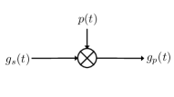
Figure 1: Impulse-train sampling [19, Page 516]. The sampling of the signal $g_{s}(t)$ leads to $g_{p}(t)$, which is represented by the multiplication of $g_{s}(t)$ and sampling function $p(t)=\sum_{k=-\infty}^{\infty}\delta(t-kT_{s})$, where $T_{s}$ is sampling period.

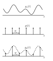
(a)

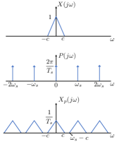
(b)

Figure 2: Effect of impulse-train sampling for band-limited signal in time (a) and frequency domain (b) [19, Page 516-518].

The Nyquist-Shannon sampling theorem states the basic result of this question for band-limited signals with the maximum frequency $\omega_{M}=c$ (rad/s). Specifically, the multiplication of $g_{s}(t)$ and $p(t)$ in the time domain corresponds to convolution of associated Fourier transforms in frequency domain, i.e., $X(j\omega)$ and $P(j\omega)$. Then we denote the resulted Fourier transform of $g_{p}(t)$ as $X_{p}(j\omega)$. This effect of sampling is characterized in time and frequency domain in Fig. 2a and Fig. 2b, respectively. As Fig. 2b shows, when $\omega_{s}>2c$, $X(j\omega)$ can be faithfully reproduced without overlap. And the CT signal $g_{s}(t)$ can be exactly reconstructed from samples by a suitable lowpass filter [19, Page 516-518].

II-B The Koopman operator

Here we introduce basic properties of the Koopman operator $U^{\tau},\tau\geq 0$ for signal description. Consider the semigroup of the Koopman operator [14] defined as follows

$$U^{\tau}g=g\circ S^{\tau},\,\,g\in\mathcal{F},$$ (1)

where $g:\mathbb{R}\to\mathbb{C}$ is a function that belongs to the Banach space $\mathcal{F}$ and $S^{\tau}(t)=t+\tau$ is the flow of time $t\in\mathbb{R}$. Koopman operator is a linear operator, i.e., let the signal functions $g_{1},g_{2}\in\mathcal{F}$,

$$U^{\tau}(\alpha_{1}g_{1}+\alpha_{2}g_{2})=\alpha_{1}U^{\tau}g_{1}+\alpha_{2}U^{\tau}g_{2},\ \alpha_{1},\alpha_{2}\in\mathbb{R}.$$

Therefore, the Koopman operator describes the evolution of signal functions in $\mathcal{F}$ in terms of linear transformation.

The infinitesimal generator $L$ of the Koopman operator is also a linear operator, which is defined as:

$$Lg=\lim_{\tau\to 0^{+}}\frac{1}{\tau}(U^{\tau}-I)g,\ g\in\mathcal{D}(L).$$ (2)

So $Lg$ can be seen as the “derivative” of the signal function $g$ with respect to time, i.e., $\dot{g}=Lg$, where $\dot{g}$ denotes $\partial(g\circ S^{\tau})/\partial{\tau}$[20].

When the Koopman operator $U^{\tau}$ and its generator $L$ are both bounded, we have

$$U^{\tau}=e^{L\tau}.$$

Besides, the spectrum also admits this exponential relationship [21, Lemma 3.13], i.e.,

$$\sigma(U^{\tau})=\{e^{\lambda\tau}:\tau\in\sigma(L)\}.$$

In the following, we also call $\sigma(L)$ as Koopman spectrum.

Here we introduce some definitions of the spectrum of linear operator $B\in\mathcal{L}(X)$. Let $I$ be the identity operator on $\mathcal{F}$. The spectrum $\sigma(B)$ is the set of all $\lambda\in\mathbb{C}$ for which the operator $B-\lambda I$ does not have an inverse. The point spectrum $\sigma_{p}(B)$ is the set of value $\lambda$ such that $B-\lambda I$ is not injective, where $I$ is the identity operator. When the Koopman operator $U^{\tau}$ admits point spectrum, the eigenvalue and associated eigenfunction of the Koopman operator are defined as below.

Definition 1 (Koopman eigenvalues and eigenfunctions).

An eigenvalue of the Koopman operator is the value $\lambda_{k}\in\mathbb{C}$ that:

$$U^{\tau}\phi_{k}=e^{\lambda_{k}\tau}\phi_{k},$$

where $\phi_{k}\in\mathcal{F},\phi_{k}\neq 0$ is associated Koopman eigenfunction.

The Koopman eigenfunction $\phi_{k}$ is also an eigenfunction of the generator $L$, i.e.,

$$L\phi_{k}=\lambda_{k}\phi_{k},$$

where $\lambda_{k}$ is associated eigenvalue of the generator $L$, and it belongs to its point spectrum $\sigma_{p}(L)$.

III Signals in generator-bounded space

We address the sampling theorem for signals $g_{s}(t)$ belonging to generator-bounded space $\mathcal{F}_{e}$. Thus, we first present the definition and properties of $g_{s}\in\mathcal{F}_{e}$ in Section III-A. Also, we provide two examples of such signals for illustration, i.e., the inverse-Laplace type of signals and linear combinations of exponential and polynomial signals in Section III-B and Section III-C, respectively.

III-A Generator-bounded space

Consider a signal $g_{s}\in\mathcal{F}_{e}$, where the generator-bounded space $\mathcal{F}_{e}$ is defined as follows.

Definition 2 (Generator-bounded space $\mathcal{F}_{e}$).

The generator-bounded space $\mathcal{F}_{e}$ is a separable Banach space that satisfies

• The space $\mathcal{F}_{e}$ is invariant under the Koopman operator $U^{\tau}$, i.e., $\forall g\in\mathcal{F}_{e},\forall\tau\geq 0$, we have $U^{\tau}g\in\mathcal{F}_{e}$.

• The restriction of the Koopman operator $U^{\tau}|_{\mathcal{F}_{e}}$ and its generator $L|_{\mathcal{F}_{e}}$ are bounded, i.e., $\|U^{\tau}|_{\mathcal{F}_{e}}\|,\|L|_{\mathcal{F}_{e}}\|<\infty$.

Here we show the property that the signal $g_{s}(t)$ belonging to $\mathcal{F}_{e}$ oscillates with finite frequency and finite growth rate of amplitude at $t<\infty$. Since $g_{s}\in\mathcal{F}_{e}$ and $\mathcal{F}_{e}$ is an invariant space of the Koopman operator, the value of the signal $g_{s}(t)$ at $t=\tau$ is represented by the Koopman operator $U^{\tau}|_{\mathcal{F}_{e}}$, i.e.,

$$g_{s}(\tau)=U^{\tau}|_{\mathcal{F}_{e}}g_{s}(0)=e^{L|_{\mathcal{F}_{e}}\tau}g_{s}(0).$$

When $\mathcal{F}_{e}$ is infinite-dimensional, it follows from the functional calculus that

$$g_{s}(\tau)=U^{\tau}|_{\mathcal{F}_{e}}g_{s}(0)=\int_{\sigma(L|_{\mathcal{F}_{e}})}e^{\lambda\tau}E({\rm d}\lambda)g_{s}(0),$$ (3)

where $E$ is the resolution of the identity for $L|_{\mathcal{F}_{e}}$ [22, P. 898]. Besides, when $\mathcal{F}_{e}$ is finite-dimensional, i.e., $\mathcal{F}_{e}=\mathrm{span}\{\phi_{1},\ldots,\phi_{n}\}$ with the spectrum $\sigma(L|_{\mathcal{F}_{e}})=\{\lambda_{k}\}_{k=1}^{n}$, then $g_{s}(\tau)$ is determined by

$$g_{s}(\tau)=U^{\tau}|_{\mathcal{F}_{e}}g_{s}(0)=\sum_{k=1}^{n}e^{\lambda_{k}\tau}E(\lambda_{k})g_{s}(0).$$ (4)

Hence the oscillation and growth of amplitude are characterized by the real and imaginary parts of $\lambda\in\sigma(L|_{\mathcal{F}_{e}})$, respectively. Based on the theorem of spectral radius [21, P. 241], i.e.,

$$r_{\sigma}(L|_{\mathcal{F}_{e}})\leq\|L|_{\mathcal{F}_{e}}\|,$$

where the spectral radius $r_{\sigma}(L|_{\mathcal{F}_{e}}):=\sup\{|\lambda|:\lambda\in\sigma(L|_{\mathcal{F}_{e}})\}$, we have bounded spectrum $\sigma(L|_{\mathcal{F}_{e}})$ because $\|L|_{\mathcal{F}_{e}}\|<\infty$. So the signal $g_{s}(t)\in\mathcal{F}_{e}$ oscillates with a finite frequency and finite growth rate of amplitude for $t<\infty$.

Intuitively, the generator-bounded space $\mathcal{F}_{e}$ generalizes the space of band-limited signal. This is because that, the dimensionality to characterize signal properties is increased by converting from one-dimensional Fourier spectrum to two-dimensional Koopman spectrum, i.e., from $\omega\in\mathbb{R}$ to $\lambda\in\mathbb{C}$. Specifically, band-limited signal is determined by limited Fourier frequency domain. It can be described by a bounded Koopman spectrum with only one axis of complex space $\mathbb{C}$, which indicates the oscillation with finite frequency and no amplitude growth. On another axis of $\mathbb{C}$, however, other signals in $\mathcal{F}_{e}$ can have non-zero representations. The detail will be further demonstrated for non-periodic and periodic band-limited signals in Section III-B and Section III-C respectively.

III-B Inverse-Laplace type of signals

Here we present the inverse-Laplace type of the signal as an example of $g_{s}\in\mathcal{F}_{e}$, i.e., $g_{s}(t)=\int_{-c}^{c}F(\omega)e^{(\alpha+i\omega)t}{\rm d}\omega$, where $F(\omega)\in L^{2}[-c,c],c\geq 0$. Particularly, non-periodic band-limited signal is a special case of such signals.

Before proving that inverse-Laplace type of the signal $g_{s}(t)$ belongs to $\mathcal{F}_{e}$, we need a lemma to show the property of $g(t)=\int_{-c}^{c}h(\omega)e^{i\omega t}{\rm d}\omega,$ where $h(\omega)\in L^{2}[-c,c]$.

Lemma 1 (Parseval’s Theorem).

If the function $g(t)=\int_{-c}^{c}h(\omega)e^{i\omega t}{\rm d}\omega$, where $h(\omega)\in L^{2}[-c,c]$, then

$$\int_{-\infty}^{\infty}|g(t)|^{2}{\rm d}t=\int_{-c}^{c}|h(\omega)|^{2}{\rm d}\omega.$$

Then we use the Lemma 1 to prove that $g_{s}\in\mathcal{F}_{e}$ as below.

Proposition 1 (Inverse-Laplace type of signal).

The inverse-Laplace type of signal $g_{s}(t)=\int_{-c}^{c}F(\omega)e^{(\alpha+i\omega)t}{\rm d}\omega$, where $F(\omega)\in L^{2}[-c,c]$ and $c>0,\alpha\in\mathbb{R}$, belongs to the generator-bounded space

$$\mathcal{F}_{e}=\left\{g(t)=\int_{-c}^{c}h(\omega)e^{(\alpha+i\omega)t}{\rm d}\omega:h(\omega)\in L^{2}[-c,c]\right\}.$$

with the spectrum $\sigma(L|_{\mathcal{F}_{e}})=\alpha+i[-c,c]$.

Proof.

By the definition of the signal, the signal $g_{s}(t)$ belongs to $\mathcal{F}_{e}=\left\{g(t)=\int_{-c}^{c}h(\omega)e^{(\alpha+i\omega)t}{\rm d}\omega:h(\omega)\in L^{2}[-c,c]\right\}$.

Then we show that $\mathcal{F}_{e}$ is a generator-bounded space. Let $\|g\|=(\int_{-\infty}^{\infty}|g(t)e^{-\alpha t}|^{2}{\rm d}t)^{1/2}$. Consider Cauchy sequence $\{g_{n}\}\subset\mathcal{F}_{e}$, where

$$g_{n}(t)=\int_{-c}^{c}h_{n}(\omega)e^{(\alpha+i\omega)t}{\rm d}\omega,h_{n}(\omega)\in L^{2}[-c,c].$$

Then, for $\forall\epsilon>0$, there exists $N>0$, such that

$$\int_{-\infty}^{\infty}|(g_{n}(t)-g_{m}(t))e^{-\alpha t}|^{2}{\rm d}x<\epsilon,~{}\forall n,m>N.$$ (5)

Let $\hat{g}_{n}(t)=g_{n}(t)e^{-\alpha t},\hat{g}_{m}(t)=g_{m}(t)e^{-\alpha t}$. It follows (5) that $\{\hat{g}_{n}\}$ is a Cauchy sequence of Banach space

$$\widehat{\mathcal{F}}=\left\{g(t)=\int_{-c}^{c}h(\omega)e^{i\omega t}{\rm d}t:h(\omega)\in L^{2}[-c,c]\right\},$$

with the $l^{2}-$norm. Then we have the convergence of $\hat{g}_{n}\stackrel{{\scriptstyle l^{2}}}{{\longrightarrow}}\hat{g}\in\widehat{\mathcal{F}}$, i.e., for $\forall\epsilon>0,$ there exists $N>0$, such that

$$\int_{-\infty}^{\infty}|g_{n}(t)e^{-\alpha t}-\hat{g}(t)|^{2}{\rm d}t<\epsilon,~{}\forall n>N.$$

So we have the convergence of the Cauchy sequence in $\mathcal{F}_{e}$, i.e., $g_{n}\to g$, where $g(t)=\hat{g}(t)e^{\alpha t}=\int_{-c}^{c}h(\omega)e^{(\alpha+i\omega)t}\in\mathcal{F}_{e}$. Therefore, $\mathcal{F}_{e}$ is a Banach space and it has basis functions $\{e^{\alpha t}\hat{\phi}_{k}(t)\}_{k\in\mathbb{Z}}$, where $\{\hat{\phi}_{k}(t)\}_{k\in\mathbb{Z}}$ are basis functions of $\widehat{\mathcal{F}}$.

Then we show that the Koopman operaor $U^{\tau}$ is invariant on $\mathcal{F}_{e}$. For $\forall\tau>0,\forall g\in\mathcal{F}_{e}$ we have

$$U^{\tau}g(t)=g\circ S^{\tau}(t)=\int_{-c}^{c}h(\omega)e^{(\alpha+i\omega)\tau}e^{(\alpha+i\omega)t}{\rm d}\omega.$$

Since $e^{(\alpha+i\omega)\tau}h(\omega)\in L^{2}[-c,c]$, we have $U^{\tau}g\in\mathcal{F}_{e}$.

Here we prove that the restriction of the generator $L|_{\mathcal{F}_{e}}$ is bounded.

$$\|L|_{\mathcal{F}_{e}}\| =\sup_{\|g\|=1}\left\|\frac{{\rm d}g}{{\rm d}t}\right\|=\sup_{\|g\|=1}\left(\int_{-\infty}^{\infty}\left|\frac{{\rm d}g(t)}{{\rm d}t}e^{-\alpha t}\right|^{2}{\rm d}t\right)^{1/2}$$

$$=\sup_{\|g\|=1}\left(\int_{-\infty}^{\infty}\left|\int_{-c}^{c}(\alpha+i\omega)h(\omega)e^{i\omega t}{\rm d}\omega\right|^{2}{\rm d}t\right)^{1/2}.$$

Based on Lemma 1, we have

$$\|L|_{\mathcal{F}_{e}}\| =\sup_{\|g\|=1}\left(\int_{-c}^{c}(\alpha^{2}+\omega^{2})|h(\omega)|^{2}{\rm d}\omega\right)^{1/2}$$

$$\leq\sup_{\|g\|=1}\left((\alpha^{2}+c^{2})\int_{-c}^{c}|h(\omega)|^{2}{\rm d}\omega\right)^{1/2}.$$

It follows Lemma 1 that $\|g\|=(\int_{-c}^{c}|h(\omega)|^{2}{\rm d}\omega)^{1/2}.$ Therefore, we obtain that

$$\|L|_{\mathcal{F}_{e}}\|\leq\sqrt{\alpha^{2}+c^{2}}<\infty.$$

We can similarly prove that $\|U^{\tau}|_{\mathcal{F}_{e}}\|<\infty$ for $\forall\tau>0$.

Finally we prove that $\sigma(L|_{\mathcal{F}_{e}})=\alpha+i[-c,c]$ by demonstrating that the resolvent set $\rho(L|_{\mathcal{F}_{e}})$ is $\mathbb{C}/(\alpha+i[-c,c])$. Based on the definition [21, Def 1.1] of resolvent set $\rho(L|_{\mathcal{F}_{e}})$, the operator $\lambda I-L|_{\mathcal{F}_{e}}:\mathcal{F}_{e}\to\mathcal{F}_{e}$ is bijective for $\forall\lambda\in\rho(L|_{\mathcal{F}_{e}})$ and $\sigma(L|_{\mathcal{F}_{e}})=\mathbb{C}/\rho(L|_{\mathcal{F}_{e}})$. So we consider that $\lambda I-L|_{\mathcal{F}_{e}}$ is surjective, i.e., $\forall g(t)=\int_{-c}^{c}h(\omega)e^{(\alpha+i\omega)t}{\rm d}\omega\in\mathcal{F}_{e}$, there exists $\hat{g}(t)=\int_{-c}^{c}\hat{h}(\omega)e^{(\alpha+i\omega)t}{\rm d}\omega\in\mathcal{F}_{e}$ such that

$$(\lambda I-L|_{\mathcal{F}_{e}})\hat{g}=g.$$

It follows that $\hat{h}(\omega)=h(\omega)/(\lambda-\alpha-i\omega)$ for $\forall h\in L^{2}[-c,c]$. Then we have $\lambda\in\mathbb{C}/(\alpha+i[-c,c])$. Similarly, the sufficiency can be proved, i.e., $(\lambda I-L|_{\mathcal{F}_{e}})$ is surjective if $\lambda\in\mathbb{C}/(\alpha+i[-c,c])$. Thus, the resolvent set $\rho(L|_{\mathcal{F}_{e}})\subseteq\mathbb{C}/(\alpha+i[-c,c])$. Then we show that $(\lambda I-L|_{\mathcal{F}_{e}})$ is also injective for $\forall\lambda\in\mathbb{C}/(\alpha+i[-c,c])$, i.e.,

$$(\lambda I-L|_{\mathcal{F}_{e}})g=\int_{-c}^{c}(\lambda-\alpha-i\omega)h(\omega)e^{(\alpha+i\omega)t}{\rm d}\omega=0$$ (6)

$$\Rightarrow g(t)=\int_{-c}^{c}h(\omega)e^{(\alpha+i\omega)t}{\rm d}\omega=0,~{}\forall t>0.$$ (7)

It follows (6) that $\dot{g}(t)=\lambda g(t)$ and $g(t)=e^{\lambda t}g(0)$, i.e.,

$$\int_{-c}^{c}e^{(\alpha+i\omega)t}h(\omega){\rm d}\omega=e^{\lambda t}g(0),~{}\forall t>0.$$

For $\forall\lambda\in\mathbb{C}/(\alpha+i[-c,c])$, it holds only when $g(t)=0$, which is consistent with (7). Then $(\lambda I-L|_{\mathcal{F}_{e}})$ is also injective for $\forall\lambda\in\mathbb{C}/(\alpha+i[-c,c])$. Therefore, the resolvent set is $\rho(L|_{\mathcal{F}_{e}})=\mathbb{C}/(\alpha+i[-c,c])$ and the spectrum is $\sigma(L|_{\mathcal{F}_{e}})=\alpha+i[-c,c]$.

∎

Remark 1 (Non-periodic band-limited signal).

When $\alpha=0$, it is clear that the non-periodic band-limited signal $g_{s}(t)=\int_{-c}^{c}F(\omega)e^{i\omega t}{\rm d}\omega$, where $F(\omega)\in L^{2}[-c,c],$ is a particular case of inverse-Laplace type of signal. In this case, the Koopman spectrum is restricted to the imaginary axis and is consistent with the Fourier spectrum, i.e., $\sigma(L|_{\mathcal{F}_{e}})=i[-c,c]$.

III-C Linear combinations of polynomial and exponential signals

Besides the inverse-Laplace type, here we present another type of signals that belong to generator-bounded space $\mathcal{F}_{e}$, i.e., linear combinations of polynomial and complex exponential signal $g_{s}(t)=\sum_{k=1}^{m}\sum_{l=0}^{b_{k}}c_{k,l}t^{l}e^{\lambda_{k}t}$ where $c_{k,l},\lambda_{k}\in\mathbb{C},b_{k}\in\mathbb{N}$. We also show that periodic band-limited signal is a special case of such signals.

Here we prove that the signal $g_{s}(t)$ belongs to generator-bounded space $\mathcal{F}_{e}$.

Proposition 2 (Polynomial and exponential signals).

The signal $g_{s}(t)=\sum_{k=1}^{m}\sum_{l=0}^{b_{k}}c_{k,l}t^{l}e^{\lambda_{k}t},$ where $c_{k,l},\lambda_{k}\in\mathbb{C},b_{k}\in\mathbb{N}$, belongs to the generator-bounded space

$$\mathcal{F}_{e}=\mathrm{span}\{ g_{1,0}(t)=e^{\lambda_{1}t},g_{1,1}(t)=te^{\lambda_{1}t},\ldots,g_{1,b_{1}}(t)=$$

$$t^{b_{1}}e^{\lambda_{1}t},g_{2,0}(t)=e^{\lambda_{2}t},\ldots,g_{m,b_{m}}(t)=t^{b_{m}}e^{\lambda_{m}t}\}.$$

with the spectrum $\sigma(L|_{\mathcal{F}_{e}})=\{\lambda_{k}\}_{k=1}^{m}$.

Proof.

By the definition of the signal, it can be proved that $g_{s}(t)$ belongs to $\mathcal{F}_{e}=\mathrm{span}\{g_{1,0}(t)=e^{\lambda_{1}t},\ldots,g_{1,b_{1}}(t)=t^{b_{1}}e^{\lambda_{1}t},g_{2,0}(t)=e^{\lambda_{2}t},\ldots,g_{m,b_{m}}(t)=t^{b_{m}}e^{\lambda_{m}t}\}.$

Then we show that $\mathcal{F}_{e}$ is a generator-bounded space. Firstly, the space $\mathcal{F}_{e}$ is a Banach space because it is spanned by finite number of basis functions. Additionally, the space is also an invariant space of the Koopman operator. Restricted in this finite-dimensional space, the generator $L|_{\mathcal{F}_{e}}$ can be represented by a matrix, i.e., $L|_{\mathcal{F}_{e}}\bm{g}=\bm{g}\overline{L}|_{\mathcal{F}_{e}}$, where $\bm{g}=[g_{1,0},\ldots,g_{1,b_{1}},g_{2,0},\ldots,g_{m,b_{m}}]$,

$$\overline{L}|_{\mathcal{F}_{e}}=\left(\begin{matrix}L_{1}&&&\\ &L_{2}&&\\ &&\ddots&\\ &&&L_{m}\end{matrix}\right),$$

and

$$L_{k}=\left(\begin{matrix}\lambda_{k}&1&&&\\ &\lambda_{k}&2&&\\ &&\ddots&\ddots&\\ &&&\lambda_{k}&b_{k}\\ &&&&\lambda_{k}\end{matrix}\right)_{(b_{k}+1)\times(b_{k}+1)}.$$

So the generator $L|_{\mathcal{F}_{e}}$, the Koopman operator $U^{\tau}|_{\mathcal{F}_{e}}=\exp(\tau L|_{\mathcal{F}_{e}})$ are both bounded. And the space $\mathcal{F}_{e}$ is a generator-bounded space. The spectrum of the generator $L|_{\mathcal{F}_{e}}$ can be obtained by the eigenvalues of $\overline{L}|_{\mathcal{F}_{e}}$, which admits point spectrum, i.e., $\sigma(L|_{\mathcal{F}_{e}})=\{\lambda_{k}\}_{k=1}^{m}$. ∎

Remark 2 (Periodic band-limited signal).

As a specific case, periodic band-limited signal is included in the linear combinations of exponential and polynomial signals, i.e., for $\forall k=1,\ldots,m,b_{k}=0$ and $\lambda_{k}=i\beta_{k},\beta_{k}\in\mathbb{R}$. In this case, the Koopman (point) spectrum $\sigma(L|_{\mathcal{F}_{e}})$ is restricted to the imaginary axis, i.e., $\sigma(L|_{\mathcal{F}_{e}})=\{i\beta_{k}\}_{k=1}^{m}$, which is consistent with the Fourier frequency.

IV Koopman operator-based sampling theorem

In this section, we prove the Koopman operator-based sampling theorem (Theorem 1) for signals $g_{s}(t)$ in generator-bounded space $\mathcal{F}_{e}$. This sampling theorem shows that $g_{s}\in\mathcal{F}_{e}$ has finite lower bound of sampling frequency $\omega_{\gamma}$ (rad/s) that avoids signal aliasing. And this lower bound is associated with imaginary part of Koopman spectrum.

Here we briefly outline the main idea to analyze the sampling theorem by the Koopman operator. We first consider the sampling problem of signal $g_{s}\in\mathcal{F}_{e}$ and the DT Koopman operator $U^{T_{s}}|_{\mathcal{F}_{e}}$ defined by DT flow $S^{T_{s}}(t)=t+T_{s}$. Secondly, we obtain the generator $L|_{\mathcal{F}_{e}}$ from $U^{T_{s}}|_{\mathcal{F}_{e}}$ without aliasing. Then the signal $g_{s}(\tau)$ can be reconstructed by $g_{s}(\tau)=U^{\tau}|_{\mathcal{F}_{e}}g_{s}(0)=e^{L|_{\mathcal{F}_{e}}\tau}g_{s}(0)$. In summary, the framework of the analysis is illustrated in Fig. 3.

Figure 3: The framework to investigate the sampling theorem of signals by the Koopman operator. The analysis consists of two steps: (1) Considering the sampling problem in generator-bounded space $\mathcal{F}_{e}$ of signal $g_{s}(t)$, (2) obtaining the generator $L|_{\mathcal{F}_{e}}$ uniquely from DT Koopman operator $U^{T_{s}}|_{\mathcal{F}_{e}}$.

Before we prove the main sampling theorem, we first introduce the essential lemma to guarantee the uniqueness of operator logarithm.

Lemma 2 (Principal logarithm[23, Thm 2]).

Consider the operator $Y\in\mathcal{L}(X)$ whose logarithm is well-defined. The principal logarithm of $Y$, denoted by $B=\mathrm{Log}(Y)$, is unique, where the spectrum $\sigma(B)\subset\mathscr{G}(B)$ and $\mathscr{G}(B)=\{z\in\mathbb{C}:-\pi<\mathrm{Im}(z)<\pi\}$.

Based on Lemma 2, here we propose the sampling theorem for signals belonging to generator-bounded space $\mathcal{F}_{e}$.

Theorem 1 (Koopman operator-based sampling theorem).

If a signal $g_{s}(t)$ belongs to generator-bounded space $\mathcal{F}_{e}$, the signal $g_{s}(t)$ can be reconstructed from its uniform samples if and only if the sampling frequency (rad/s) satisfies

$$\omega_{s}>2\min_{\mathcal{F}_{e}}\{\max|\mathrm{Im}(\sigma(L|_{\mathcal{F}_{e}}))|\}.$$ (8)

Proof.

The samples of $g_{s}(t)$ can be described by DT Koopman operator $U^{T_{s}}|_{\mathcal{F}_{e}}$, i.e., $g_{s}((k+1)T_{s})=U^{T_{s}}|_{\mathcal{F}_{e}}g_{s}(kT_{s}),k\in\mathbb{N}$. Since $U^{T_{s}}|_{\mathcal{F}_{e}}$ and its generator $L|_{\mathcal{F}_{e}}$ are both bounded, we have

$$U^{T_{s}}|_{\mathcal{F}_{e}}=\exp(L|_{\mathcal{F}_{e}}T_{s})=\sum_{k=0}^{\infty}\frac{{T_{s}}^{k}{L|_{\mathcal{F}_{e}}}^{k}}{k!}.$$

Then the generator $L|_{\mathcal{F}_{e}}$ is obtained from $U^{T_{s}}|_{\mathcal{F}_{e}}$ by operator logarithm [24, P. 172]. However, there are many solutions of the logarithm, i.e.,

$$\log(U^{T_{s}}|_{\mathcal{F}_{e}}) =\log(\exp(L|_{\mathcal{F}_{e}}T_{s}))=L|_{\mathcal{F}_{e}}T_{s}+2\pi i\sum_{k}n_{k}I_{k},$$

where $n_{k}$ are integers, $I_{k}$ denote idemponents, i.e., $\exp(2\pi iI_{k})=I$, and $I$ denotes the identity operator. Based on Lemma 2, the generator $L|_{\mathcal{F}_{e}}$ is obtained uniquely from $U^{T_{s}}|_{\mathcal{F}_{e}}$ if and only if $L|_{\mathcal{F}_{e}}T_{s}$ is principal logarithm, i.e., $L|_{\mathcal{F}_{e}}T_{s}=\mathrm{Log}(U^{T_{s}}|_{\mathcal{F}_{e}})$. It follows that the spectrum of $T_{s}L|_{\mathcal{F}_{e}}$ lies in the strip $\{z\in\mathbb{C}:-\pi<\mathrm{Im}(z)<\pi\}$, i.e.,

$$\omega_{s}=2\pi/T_{s}>2\max|\mathrm{Im}(\sigma(L|_{\mathcal{F}_{e}}))|.$$ (9)

Since $g_{s}(\tau)=U^{\tau}|_{\mathcal{F}_{e}}g_{s}(0)$ can be reconstructed if there exists one $\mathcal{F}_{e}$ such that $L|_{\mathcal{F}_{e}}$ can be obtained from $U^{T_{s}}|_{\mathcal{F}_{e}}$. Therefore, we only require the “kernel” generator-bounded space

$$\boxed{\mathcal{F}_{e}^{\gamma}=\arg\min_{\mathcal{F}_{e}}\{\max|\mathrm{Im}(\sigma(L|_{\mathcal{F}_{e}}))|\},}$$ (10)

to satisfy the spectral condition (9). So we get the frequency condition (8). By taking $g_{s}$ as one of basis functions of $\mathcal{F}_{e}^{\gamma},$ it can be represented by the coordinate $\{c_{k}\}_{k\in\mathbb{N}^{+}},$ where $c_{1}=1$ and $c_{k}=0$ for $k\neq 1$. Then the value of $g_{s}(t)$ at $t=\tau$ can be reconstructed by

$$g_{s}(\tau)=\exp\left(\frac{\tau}{T_{s}}\mathrm{Log}(U^{T_{s}}|_{\mathcal{F}_{e}})\right)g_{s}(0).$$ (11)

∎

Therefore, the lower bound of sampling frequency $\omega_{\gamma}=2\max|\mathrm{Im}(\sigma(L|_{\mathcal{F}_{e}^{\gamma}}))|$ is related only to the imaginary part of Koopman spectrum, which reflects the oscillation frequency of the signal. According to Remark 1-2, the conclusion of Theorem 1 is consistent with Nyquist-Shannon sampling theorem for band-limited signal. For non-band-limited signals analyzed in Proposition 1-2, this finding intuitively coincides with the fact that the oscillation causes aliasing while amplitude growth rate does not. Moreover, in order to numerically realize the reconstruction (11), we propose an algorithm based on the Koopman operator in Section V.

Remark 3 (The reason of generalization).

The reason why Koopman operator-based sampling theorem extends Nyquist-Shannon sampling theorem is that, the two-dimensional spectrum of the Koopman operator is able to independently describe the oscillation that causes signal aliasing and the finite exponential growth rate of amplitude that does not. It gives the insight that, when the sampling frequency is high enough to capture the oscillation of the signal $g_{s}\in\mathcal{F}_{e}^{\gamma}$ whose growth rate is finite at $t<\infty$, the signal $g_{s}(t)$ can be definitely determined by the samples because it is the unique solution in $\mathcal{F}_{e}^{\gamma}$ that matches $g_{s}(kT_{s}),k\in\mathbb{N}$.

V Reconstruction method

For numerical realization of the sampling theorem, we propose a reconstruction algorithm with theoretical guarantee in this section. The reconstruction algorithm is described in Section V-A, and the theoretical convergence result is provided in Section V-B.

V-A Description of the method

The main idea of the reconstruction is to compute the evolution of the signal $g_{s}(t)$ by the Koopman operator $U^{\tau}:\mathcal{F}_{e}^{\gamma}\to\mathcal{F}_{e}^{\gamma}$. We first lift data to functional space $\mathcal{F}_{M}\subseteq\mathcal{F}_{e}^{\gamma}$ where $g_{s}(t)$ belongs. Then we reconstruct the signal $g_{s}(t)$ by approximating the CT Koopman operator. The specific steps are as follows.

V-A1 Lift data to functional space

With the sampling period $T_{s}$ and the DT values of the signal $\{g_{s}(kT_{s})\}_{k=1}^{N}$, the data $\{kT_{s}\}_{k=0}^{N}$ are lifted to functional space $\mathcal{F}_{M}$. The space $\mathcal{F}_{M}$ is spanned by $M$ linearly independent functions, i.e., $\mathcal{F}_{M}=\mathrm{span}\{g_{1},g_{2},\ldots,g_{M}\}$, where $g_{1}(t)=g_{s}(t)$. The basis functions $g_{k}(t),~{}k=2,\ldots,M$ can be chosen by the types of the signal. For example, the basis functions can be $g_{k}(t)=\exp(\alpha_{k}t)\cos(\beta_{k}t),\alpha_{k},\beta_{k}\in\mathbb{R}$ if the signal is assumed to be exponential.

Then we denote $\bm{g}=[g_{1},g_{2},\ldots,g_{M}]$, and construct the $N\times M$ matrices $(N>M)$.

$$X=\left(\begin{matrix}\bm{g}(0)\\ \bm{g}(T_{s})\\ \vdots\\ \bm{g}((N-1)T_{s})\end{matrix}\right),~{}Y=\left(\begin{matrix}\bm{g}(T_{s})\\ \bm{g}(2T_{s})\\ \vdots\\ \bm{g}(NT_{s})\end{matrix}\right).$$

V-A2 Approximate the Koopman operator and its generator

Here we identify the finite-rank approximation of the DT Koopman operator $\widehat{U}^{T_{s}}_{M}(N):\mathcal{F}_{M}\to\mathcal{F}_{M}$ and its generator $\widehat{L}_{M}(N):\mathcal{F}_{M}\to\mathcal{F}_{M}$. Based on Extended Dynamic Mode Decomposition [25], we obtain the matrix representation of $\widehat{U}^{T_{s}}_{M}(N)$, i.e., $\widehat{U}^{T_{s}}_{M}(N)\bm{g}=\bm{g}\overline{U}_{M}$ and

$$\overline{U}_{M}=X^{\dagger}Y.$$ (12)

The matrix representation of $\widehat{L}_{M}(N)$ can be computed as

$$\overline{L}_{M}=\log(X^{\dagger}Y)/T_{s}.$$ (13)

V-A3 Reconstruct the signal

Finally we reconstruct the signal by the approximated generator. With $g_{1}(t)=g_{s}(t)$, we have

$$g_{s}(\tau)=g_{1}\circ S^{\tau}(t)=U^{\tau}g_{1}(0),$$

where $S^{\tau}(t)=t+\tau$. By the generator $\overline{L}_{M}$, the matrix representation of the CT Koopman operator $\overline{U}_{M}^{\tau}$ is computed by

$$\overline{U}_{M}^{\tau}=\exp(\overline{L}_{M}\tau).$$

Then we reconstruct the signal by

$$\hat{g}_{s}(\tau)=\hat{g}_{1}(\tau)=\bm{g}(0)(\overline{U}^{\tau}_{M}\bm{e}_{1}),$$

where $\bm{e}_{1}=[1,0,\ldots,0]^{T}$.

Remark 4 (Connection with method of system identification).

This approach for signal reconstruction is analogous to the Koopman operator-based method of identifying nonlinear system [26]. Both of them approximate the Koopman operator in the lifted functional space $\mathcal{F}_{M}$. However, the function $g_{1}(t)=g_{s}(t)$ in $\mathcal{F}_{M}$ is unknown for signal reconstruction, which is intended to be recovered through the flow of time $S^{\tau}(t)=t+\tau$. In contrast, for system identification, all basis functions in $\mathcal{F}_{M}$ can be represented analytically. By using such learned or chosen functional space, it can recover the unknown flow $S^{\tau}({\bm{x}})$ of system states ${\bm{x}}$.

V-B Theoretical guarantee

In this section, we prove the convergence of the algorithm proposed in Section V-A in the optimal conditions.

Assume $\mathcal{F}_{M}=\mathrm{span}\{g_{1},\ldots,g_{M}\}\subseteq\mathcal{F}_{e}^{\gamma}=L^{2}[0,T_{\rm max}]$ with $l^{2}-$norm $\|\cdot\|$. We use $U^{\tau}:\mathcal{F}_{e}^{\gamma}\to\mathcal{F}_{e}^{\gamma}$ to denote the Koopman operator defined on $\mathcal{F}_{e}^{\gamma}$, $L$ to denote its generator, $P_{M}:\mathcal{F}_{e}^{\gamma}\to\mathcal{F}_{M}$ to denote the projection operator onto $\mathcal{F}_{M}$, and $U^{\tau}_{M}=P_{M}U^{\tau}|_{\mathcal{F}_{M}}:\mathcal{F}_{M}\to\mathcal{F}_{M}$ to denote the projection of the Koopman operator onto $\mathcal{F}_{M}$.

Here we show the representation of the reconstruction error by the Koopman operator. With signal function $g_{1}(t)=g_{s}(t)\in\mathcal{F}_{M}$, the value $g_{s}(\tau)$ is

$$g_{s}(\tau)=g_{1}(\tau)=U^{\tau}g_{1}(0).$$

The reconstructed signal is computed as

$$\hat{g}_{s}(\tau)=\hat{g}_{1}(\tau)=\exp\left(\frac{\tau}{T_{s}}\mathrm{Log}~{}\widehat{U}^{T_{s}}_{M}(N)\right)g_{1}(0).$$

Then the reconstruction error can be measured as

$$\left\|U^{\tau}g_{1}-\exp\left(\frac{\tau}{T_{s}}\mathrm{Log}~{}\widehat{U}^{T_{s}}_{M}(N)\right)g_{1}\right\|.$$ (14)

In order to prove the convergence of (14), we first show the continuity of exponential and logarithm functions of linear bounded operators.

Lemma 3 (Continuity of operator exponential).

Consider bounded operators $A,A_{n}\in\mathcal{L}(X).$ If $\lim_{n\to\infty}\|(A-A_{n})g\|=0,~{}\forall g\in X$, then

$$\lim_{n\to\infty}\|(\exp A-\exp A_{n})g\|=0.$$

Proof.

Since the operators $A,A_{n}$ are bounded, the exponential can be expanded by the Taylor series, i.e.,

$$\|(\exp A-\exp A_{n})g\|=\left\|\sum_{k=0}^{\infty}\frac{A^{k}-A_{n}^{k}}{k!}g\right\|,~{}\forall g\in X.$$

By the convergence of $\exp(A)$ and $\exp(A_{n})$, for any $\epsilon>0$, there exists $q>0,$ such that

$$\left\|\sum_{k=q}^{\infty}\frac{A^{k}}{k!}g\right\|<\frac{\epsilon}{3},~{}\left\|\sum_{k=q}^{\infty}\frac{A_{n}^{k}}{k!}g\right\|<\frac{\epsilon}{3}.$$

Here we show that $\lim_{n\to\infty}\|(A^{k}-A_{n}^{k})g\|=0$ for $k<q$ by mathematical induction. Consider $q=1$, we have $\lim_{n\to\infty}\|(A-A_{n})g\|=0$. Assume that $\lim_{n\to\infty}\|(A^{k}-A_{n}^{k})g\|=0$ for $k=p$. Then for $k=p+1$, we have

$$\lim_{n\to\infty}\|(A^{p+1}-A_{n}^{p+1})g\|$$

$$\leq \lim_{n\to\infty}\|(AA^{p}-AA_{n}^{p})g\|+\lim_{n\to\infty}\|(AA_{n}^{p}-A_{n}A_{n}^{p})g\|$$

$$\leq \lim_{n\to\infty}\|A\|\|(A^{p}-A_{n}^{p})g\|+\lim_{n\to\infty}\|(A-A_{n})A_{n}^{p}g\|=0.$$

It follows that,

$$\lim_{n\to\infty}\sum_{k=0}^{q-1}\|(A^{k}-A_{n}^{k})g\|=0,\forall g\in X.$$

Then for any $\epsilon>0,$ there exists $n>0$ such that

$$\lim_{n\to\infty}\sum_{k=0}^{q-1}\|(A^{k}-A_{n}^{k})g\|<\epsilon/3,$$

Therefore, for any $\epsilon>0,g\in X$, we have

$$\|(\exp A-\exp A_{n})g\|$$

$$\leq \sum_{k=0}^{q-1}\left\|\frac{A^{k}-A_{n}^{k}}{k!}g\right\|+\left\|\sum_{k=q}^{\infty}\frac{A^{k}}{k!}g\right\|+\left\|\sum_{k=q}^{\infty}\frac{A_{n}^{k}}{k!}g\right\|<\epsilon.$$

∎

Lemma 4 (Continuity of operator logarithm).

Consider bounded operators $A,A_{n}\in\mathcal{L}(X).$ If $\lim_{n\to\infty}\|(A-A_{n})g\|=0,\forall g\in X$, then

$$\lim_{n\to\infty}\|(\log A-\log A_{n})g\|=0,$$

where the logarithm is defined as

$$\log A=\frac{1}{2\pi i}\int_{+\partial\Omega}\log\lambda~{}(\lambda I-A)^{-1}{\rm d}\lambda,$$

and $+\partial\Omega$ is a smooth, positively oriented boundary of $\Omega\subset\mathbb{C}$ that $\sigma(A)\cup\sigma(A_{n})\subset\Omega$. Noted that the argument of $\lambda\in+\partial\Omega$, i.e., $\arg\lambda$, is single-valued.

Proof.

Let $\|A\|<K$, $\|A_{n}\|<K$ with $K>0$ and $\Omega=\{\lambda\in\mathbb{C}:|\lambda|<K\}$.

Consider the resolvent operator $R(\lambda,A)=(\lambda I-A)^{-1}$. Since $|\lambda|>\|A\|$ and $|\lambda|>\|A_{n}\|$ for $\lambda\in+\partial\Omega$, the resolvent operator is expanded by the series below [27, P. 584]

$$R(\lambda,A)=\sum_{k=0}^{\infty}\frac{A^{k}}{\lambda^{k+1}},~{}R(\lambda,A_{n})=\sum_{k=0}^{\infty}\frac{A_{n}^{k}}{\lambda^{k+1}}.$$

By the convergence of these series and $\lim_{n\to\infty}\|(A-A_{n})g\|=0$, we can prove that

$$\lim_{n\to\infty}\|(R(\lambda,A)-R(\lambda,A_{n}))g\|=\lim_{n\to\infty}\|\sum_{k=0}^{\infty}\frac{A^{k}-A_{n}^{k}}{\lambda^{k+1}}g\|=0,$$

which is similar to the proof of Lemma 3. So, for $\forall\epsilon>0,$ there exists $n>0$ such that

$$\|(R(\lambda,A)-R(\lambda,A_{n}))g\|\leq\frac{\epsilon}{Kr},$$

where

$$r=\max_{\lambda\in+\partial\Omega}|\log\lambda|.$$

It follows that

$$\|\log A-\log A_{n})g\|$$

$$= \frac{1}{2\pi}\left\|\int_{+\partial\Omega}\log\lambda(R(\lambda,A)-R(\lambda,A_{n}))g{\rm d}\lambda\right\|$$

$$\leq \frac{1}{2\pi}\int_{+\partial\Omega}|\log\lambda|\left\|(R(\lambda,A)-R(\lambda,A_{n}))g\right\|{\rm d}\lambda$$

$$< \frac{r}{2\pi}\int_{+\partial\Omega}\frac{\epsilon}{Kr}{\rm d}\lambda=\epsilon.$$

Therefore, we have $\lim_{n\to\infty}\|(\log A-\log A_{n})g\|=0.$ ∎

Now we are ready to prove the convergence of the reconstruction at finite time horizon.

Theorem 2 (Convergence).

Assume that $\mathcal{F}_{M}=\mathrm{span}\{g_{1},g_{2},\ldots,g_{M}\}\subseteq\mathcal{F}_{e}^{\gamma}=\mathcal{L}^{2}[0,T_{\rm max}]$, where $T_{\rm max}>0$. Consider the signal $g\in\mathcal{F}_{M}$ and $\tau\in[0,T_{\rm max}]$, If the sampling frequency satisfies $\omega_{s}>2\max|\mathrm{Im}(\sigma(L))|$ (rad/s), we have

$$\lim_{M\to\infty}\lim_{N\to\infty}\left\|\left\{U^{\tau}-\exp\left(\frac{\tau}{T_{s}}\mathrm{Log}~{}\widehat{U}^{T_{s}}_{M}(N)\right)\right\}g\right\|=0.$$

Particularly, when $\mathcal{F}_{e}^{\gamma}$ is finite-dimensional, consider $\mathcal{F}_{M}=\mathcal{F}_{e}^{\gamma}=\mathrm{span}\{g_{1},g_{2},\ldots,g_{M}\}$. If sampling frequency $\omega_{s}>2\max|\mathrm{Im}(\sigma(L))|$ (rad/s), we have

$$\lim_{N\to\infty}\left\|\left\{U^{\tau}-\exp\left(\frac{\tau}{T_{s}}\mathrm{Log}~{}\widehat{U}^{T_{s}}_{M}(N)\right)\right\}g\right\|=0.$$

Proof.

When $\omega_{s}>2\max|\mathrm{Im}(\sigma(L))|$, it follows Lemma 2 that $LT_{s}$ is principal logarithm of $U^{T_{s}}$, i.e.,

$$L=\frac{1}{T_{s}}\mathrm{Log}~{}U^{T_{s}},$$

where $T_{s}=2\pi/\omega_{s}$. Since $\|U^{\tau}\|<\infty$, it follows that

$$\left\|\left\{U^{\tau}-\exp\left(\frac{\tau}{T_{s}}\mathrm{Log}~{}\widehat{U}^{T_{s}}_{M}(N)\right)\right\}g\right\|$$

$$= \left\|\left\{\exp\left(\frac{\tau}{T_{s}}\mathrm{Log}~{}U^{T_{s}}\right)-\exp\left(\frac{\tau}{T_{s}}\mathrm{Log}~{}\widehat{U}^{T_{s}}_{M}(N)\right)\right\}g\right\|$$

$$\leq \left\|\left\{\exp\left(\frac{\tau}{T_{s}}\mathrm{Log}~{}U^{T_{s}}\right)-\exp\left(\frac{\tau}{T_{s}}\mathrm{Log}~{}(P_{M}U^{T_{s}}P_{M})\right)\right\}g\right\|$$

$$+ \left\|\left\{\exp\left(\frac{\tau}{T_{s}}\mathrm{Log}~{}(P_{M}U^{T_{s}}P_{M})\right)-\exp\left(\frac{\tau}{T_{s}}\mathrm{Log}~{}U^{T_{s}}_{M}\right)\right\}g\right\|$$

$$+ \left\|\left\{\exp\left(\frac{\tau}{T_{s}}\mathrm{Log}~{}U^{T_{s}}_{M}\right)-\exp\left(\frac{\tau}{T_{s}}\mathrm{Log}~{}\widehat{U}^{T_{s}}_{M}(N)\right)\right\}g\right\|.$$

Here we show that these three terms in the last inequality tend to zero as $N\to\infty$ and $M\to\infty$ for $\mathcal{F}_{e}^{\gamma}=\mathcal{L}^{2}[0,T_{max}]$. Since the identified Koopman operator $\widehat{U}^{T_{s}}_{M}(N)$ conveges to $U^{T_{s}}_{M}$ as $N\to\infty$ for any norm [28], we have

$$\lim_{N\to\infty}\|U^{T_{s}}_{M}g-\widehat{U}^{T_{s}}_{M}(N)g\|=0,~{}\forall g\in\mathcal{F}_{M}.$$

It follows Lemma 4 that

$$\lim_{N\to\infty}\|\mathrm{Log}U^{T_{s}}_{M}g-\mathrm{Log}\widehat{U}^{T_{s}}_{M}(N)g\|=0.$$

By Lemma 3 and $\tau<\infty$, we have

$$\lim_{N\to\infty}\left\|\left\{\exp\left(\frac{\tau}{T_{s}}\mathrm{Log}~{}U^{T_{s}}_{M}\right)-\exp\left(\frac{\tau}{T_{s}}\mathrm{Log}~{}\widehat{U}^{T_{s}}_{M}(N)\right)\right\}g\right\|$$

$$=0.$$

Since the projection operator $P_{M}$ converges to identity operator $I$ in the strong operator topology as $M\to\infty$. So we have, $\forall g\in\mathcal{F}_{M}$,

$$\lim_{M\to\infty}\left\|(U^{T_{s}}-P_{M}U^{T_{s}}P_{M})g\right\|$$

$$\leq \lim_{M\to\infty}\left\{\left\|(U^{T_{s}}-P_{M}U^{T_{s}})g\right\|+\left\|(P_{M}U^{T_{s}}-P_{M}U^{T_{s}}P_{M})g\right\|\right\}$$

$$= \lim_{M\to\infty}\left\{\left\|(I-P_{M})U^{T_{s}}g\right\|+\left\|P_{M}U^{T_{s}}(I-P_{M})g\right\|\right\}=0.$$

Additionally, it follows $P_{M}g=g,U_{M}^{T_{s}}g=P_{M}U^{T_{s}}g$ for $\forall g\in\mathcal{F}_{M}$ that

$$\lim_{M\to\infty}\left\|(P_{M}U^{T_{s}}P_{M}-U_{M}^{T_{s}})g\right\|=0.$$

Based on Lemma 3-4, it follows that

$$\left\|\left\{\exp\left(\frac{\tau}{T_{s}}\mathrm{Log}~{}U^{T_{s}}\right)-\exp\left(\frac{\tau}{T_{s}}\mathrm{Log}~{}(P_{M}U^{T_{s}}P_{M})\right)\right\}g\right\|$$

tends to zero as $M\to\infty$, and

$$\left\|\left\{\exp\left(\frac{\tau}{T_{s}}\mathrm{Log}~{}(P_{M}U^{T_{s}}P_{M})\right)-\exp\left(\frac{\tau}{T_{s}}\mathrm{Log}~{}U^{T_{s}}_{M}\right)\right\}g\right\|$$

tends to zero as $M\to\infty$. Therefore, we have

$$\lim_{M\to\infty}\lim_{N\to\infty}\left\|\left\{U^{\tau}-\exp\left(\frac{\tau}{T_{s}}\mathrm{Log}~{}\widehat{U}^{T_{s}}_{M}(N)\right)\right\}g\right\|=0.$$

When the finite-dimensional space satisfies $\mathcal{F}_{M}=\mathcal{F}_{e}^{\gamma}$, we have $P_{M}=I$. It can be proved similarly that

$$\lim_{N\to\infty}\left\|\left\{U^{\tau}-\exp\left(\frac{\tau}{T_{s}}\mathrm{Log}~{}\widehat{U}^{T_{s}}_{M}(N)\right)\right\}g\right\|=0.$$

∎

Therefore, Theorem 2 shows that the reconstruction over finite time horizon based on the Koopman operator is asymptotically exact when $\omega_{s}>2|\mathrm{Im}(\sigma(L))|$ (rad/s) and $M,N\to\infty$ for $\mathcal{F}_{e}^{\gamma}=L^{2}[0,T_{\rm max}]$, or $N\to\infty$ for finite-dimensional $\mathcal{F}_{M}=\mathcal{F}_{e}^{\gamma}$.

VI Numerical examples

In this section, we provide several examples of signals to illustrate Theorem 1 and the reconstruction algorithm, including band-limited and non-band-limited signals.

We show that, the signal is successfully recovered when (8) is satisfied, and the aliasing exists when it does not hold. Here we just manually choose the basis functions of certain types signals to numerically illustrate Theorem 1. The improvement of this reconstruction algorithm by data-driven learning of the invariant space will be studied in the further research.

VI-1 Band-limited signal

Consider a band-limited signal

$$g_{s}(t)=-\cos(2t)+\cos(0.5t+\pi/2)+1.5\cos(4t+\pi/3).$$

The experimental settings are as follow. According to Nyquist-Shannon sampling theorem and Theorem 1, the sampling condition of this signal is $\omega_{s}>8$ rad/s. The critical sampling period is $T_{\gamma}\approx 0.785$s. Thus, we use $16$ samples with sampling periods $0.78$s and $0.79$s for illustration, respectively. For the functional space, we choose the basis functions $g_{1}(t)=g_{s}(t),~{}g_{2}(t)=\sin(2t),~{}g_{3}(t)=\cos(t),~{}g_{4}(t)=\sin(t),~{}g_{5}(t)=\cos(0.5t+\pi/2),~{}g_{6}(t)=\sin(0.5t+\pi/2),~{}g_{7}(t)=\cos(0.25t+\pi/2),~{}g_{8}(t)=\sin(0.25t+\pi/2),\ldots,~{}g_{11}=\cos(2t+\pi/3),~{}g_{12}=\sin(2t+\pi/3).$

The reconstruction results are illustrated in Fig. 4a and Fig. 4b for the sampling periods of samples $T_{s}=0.78$s and $T_{s}=0.79$s, respectively. In these figures, the triangles denote the samples and the blue line denotes the signal $g_{s}(t)$. The reconstructed signal $\hat{g}_{s}(t)$ is denoted by orange dashed line. It shows that, the signal is successfully reconstructed from the samples when the sampling period is $T_{s}=0.78<T_{\gamma}$ as Fig. 4a. This is consistent with Theorem 1. And when the sampling period is $T_{s}=0.79>T_{\gamma}$, the reconstruction fails and signal aliasing exists as Fig. 4b, where the value of $\hat{g}_{s}(t)$ is consistent with the original signal only at the sampling moments.

Here we show errors $e_{1}(t)$, $e_{2}(t)$, which are computed as

$$e_{1}(t)=|g_{s}(t)-\hat{g}^{(1)}_{s}(t)|,$$ (15)

$$e_{2}(t)=|g_{s}(t)-\hat{g}^{(2)}_{s}(t)|,$$

where $\hat{g}^{(1)}_{s}(t)$ and $\hat{g}^{(2)}_{s}(t)$ denote reconstructed signal from samples of sampling period $T_{s}=0.78$s and $T_{s}=0.79$s, respectively. Then the error is shown in Fig. 4c. These results show that when signal aliasing exists, the reconstruction error is only negligible at sampling moments, and and that at other times, the values of the two signals are quite distinct.

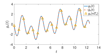
(a)

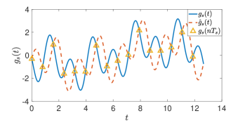
(b)

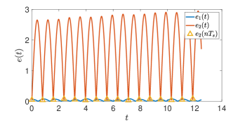
(c)

Figure 4: Reconstruction of the band-limited signal from the samples of sampling period $T_{s}=0.78$s (a), $T_{s}=0.79$s (b), and their reconstruction error (c).

VI-2 Exponential signals

Here we consider exponential signals which is non-band-limited

$$g_{s}(t)=e^{t}\cos(4t+\pi/6)+e^{0.5t}\cos(2t).$$

The experimental settings are as follow. This type of signal is analyzed in Proposition 2 and the associated Koopman spectrum is $\{1\pm 4i,0.5\pm 2i\}$. Then the critical sampling period of this signal is $T_{\gamma}\approx 0.785$s based on Theorem 1. Thus, we also use $16$ samples with the sampling period $0.78$s and $0.79$s for reconstruction. And we choose basis functions $g_{1}(t)=g_{s}(t),g_{2}(t)=e^{t}\sin(4t+\pi/6),g_{3}(t)=e^{t}\cos(2t+\pi/6),g_{4}(t)=e^{t}\sin(2t+\pi/6),g_{5}(t)=e^{t}\cos(t+\pi/6),g_{6}(t)=e^{t}\sin(t+\pi/6),g_{7}(t)=e^{0.5t}\cos(2t),\ldots,g_{12}=e^{0.5t}\sin(0.5t).$

The reconstruction results are illustrated in Fig. 5a and Fig. 5b for $T_{s}=0.78$s and $T_{s}=0.79$s, respectively. In these figures, the triangles and blue line denote the samples and signal $g_{s}(t)$. The reconstructed signal $\hat{g}_{s}(t)$ from the samples is denoted by orange dashed line. The signal is effectively reconstructed when sampling period is $T_{s}=0.78<T_{\gamma}$ as shown in Fig. 5a. Additionally, the reconstruction fails when the sampling period is $T_{s}=0.79$ as shown in Fig. 5b, which is a little longer than $T_{\gamma}$.

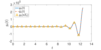
(a)

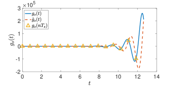
(b)

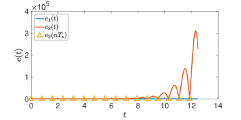
(c)

Figure 5: Reconstruction of the non-band-limited signal related to exponential functions from the samples of sampling period $T_{s}=0.78$s (a), $T_{s}=0.79$s (b), and their reconstruction error (c).

The values of the error $e_{1}(t)$ and $e_{2}(t)$ computed by (15) are illustrates in Fig. 5c. It shows that the value of $e_{1}(t)$ remains small, while $e_{2}(t)$ is only small at sampling moments. This phenomenon is evident at $t>8$s, because the exponential growth of the amplitude causes the range of $y-$axis to be too wide to distinguish between the original signal and the reconstructed signal at $t<8$.

VI-3 Polynomial and fourier signal

We consider the non-band-limited signal related to polynomial and sine functions

$$g_{s}(t)=-t^{2}\cos(4t+\pi/3)+t\cos(2t).$$

Here is the experimental setting. According to Proposition 2, the Koopman spectrum is $\sigma(L|_{\mathcal{F}_{e}^{\gamma}})=\{\pm 4i,\pm 2i\}$. Based on Theorem 1, the critical sampling period is $T_{\gamma}\approx 0.785$s. We also use $16$ samples with the sampling period $0.78$s and $0.79$s for reconstruction. And we choose these basis functions for functional space $g_{1}(t)=g_{s}(t),g_{2}(t)=t^{2}\sin(4t+\pi/3),g_{3}(t)=t\cos(4t+\pi/3),g_{4}(t)=t\sin(4t+\pi/3),g_{5}(t)=\cos(4t+\pi/3),g_{6}(t)=\sin(4t+\pi/3),\ldots,g_{10}=\sin(2t).$

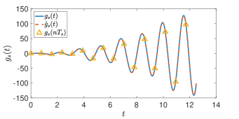
(a)

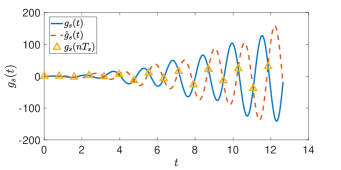
(b)

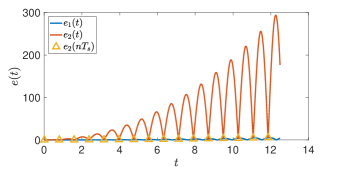
(c)

Figure 6: Reconstruction of the non-band-limited signal related to polynomial and sine functions from the samples of sampling period $T_{s}=0.78$s (a), $T_{s}=0.79$s (b), and their reconstruction error (c).

The reconstruction results are illustrated in Fig. 6a and Fig. 6b with $T_{s}=0.78$s and $T_{s}=0.79$s, respectively. In these figures, the triangles and the blue line denote the samples and original signal $g_{s}(t)$, respectively. The reconstructed signal $\hat{g}_{s}(t)$ is denoted by orange dashed line. The signal is successfully reconstructed when $T_{s}<T_{\gamma}$ as Fig. 6a. However, when the sampling condition of Theorem 1 is not satisfied, the reconstructed signal also fits the samples but is distinctly different from the original signal, as showed in Fig. 6b.

We also show the value of the error in Fig. 6c, where $e_{1}(t)$ and $e_{2}(t)$ are computed by (15). It also demonstrates that when the sampling condition is not satisfied, i.e., $Ts=0.79$s, the error at sampling moments is small while the error at other moments can not be ignored. The distinction between $g_{s}(t)$ and $\hat{g}_{s}^{(2)}(t)$ becomes apparent as $|g_{s}(t)|$ increases.

VI-4 Exponential, polynomial and sine functions

Then we consider the non-band-limited signal related to polynomial, exponential and sine functions

$$g_{s}(t)=te^{-t}\cos(4t+\pi/3).$$

(a)

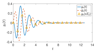
(b)

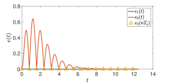
(c)

Figure 7: Reconstruction of the non-band-limited signal related to polynomial, exponential and sine functions from the samples of sampling period $T_{s}=0.78$s (a), $T_{s}=0.79$s (b), and their reconstruction error (c).

Here is the experimental setting. According to Proposition 2 and Theorem 1, we have the critical sampling period $T_{\gamma}\approx 0.785$s. Thus, we sampled $16$ samples with the sampling period $0.78$s and $0.79$s for reconstruction, respectively. And we choose these basis functions for functional space $g_{1}(t)=g_{s}(t),~{}g_{2}(t)=te^{-t}\sin(4t+\pi/3),~{}g_{3}(t)=te^{-t}\cos(2t+\pi/3),~{}g_{4}(t)=te^{-t}\sin(2t+\pi/3),~{}g_{5}(t)=te^{-t}\cos(t+\pi/3),~{}g_{6}(t)=te^{-t}\sin(t+\pi/3),~{}g_{7}(t)=e^{-t}\cos(4t+\pi/3),\ldots,~{}g_{12}({\bm{x}})=e^{-t}\sin(t+\pi/3).$

The reconstruction results are illustrated in Fig. 7a and Fig. 7b for $T_{s}=0.78$s and $T_{s}=0.79$s, respectively. In these figures, the triangles, blue line, and orange line denote the samples, original $g_{s}(t)$ and the reconstructed signal $\hat{g}_{s}(t)$, respectively. It also shows that, this signal is successfully reconstructed when sampling period is $T_{s}=0.78<T_{\gamma}$ as Fig. 7a. And when $T_{s}=0.79>T_{\gamma}$, the reconstruction fails as Fig. 7b. Similar to the result in Fig. 4b-Fig. 6b, the reconstructed signal that matches the samples of associated sampling period is distinctly different from original signal.

The value of the error (15) is illustrated in Fig. 4c. It shows that the reconstruction error is not small at non-sampling moments when (8) is not satisfied. The error $e_{2}(t)$ becomes smaller with the growing $t$ because the $|g_{s}(t)|$ tends to $0$.

Remark 5 (Functional space $\mathcal{F}_{M}$ in the algorithm).

The performance of the Koopman operator-based reconstruction algorithm depends on Koopman invariance of the functional space $\mathcal{F}_{M}$. Therefore, choosing appropriate basis functions $\{g_{k}\}_{k=2}^{M}$ is crucial. In this work, we manually select the basis functions for each type of the signal to illustrate the sampling theorem. Actually, there has been a lot of data-driven work that learns the invariant subspace and the representation of the Koopman operator from data [29, 30, 31], which will be helpful to improve this reconstruction algorithm.

VII CONCLUSIONS

In this paper, we propose a Koopman operator-based sampling theorem for signals in generator-bounded space, showing that the lower bound of sampling frequency is related to the imaginary part of the spectrum of the generator. This theorem extends Nyquist-Shannon sampling theorem through the generalization from one-dimensional Fourier spectrum to two-dimensional Koopman spectrum, which makes band-limited signal as a special case of signals belonging to generator-bounded space. This finding also reflects that signal aliasing caused by sampling is only dependent on the oscillatory motion, which is characterized separately by the imaginary part of Koopman spectrum. Moreover, the Koopman operator-based reconstruction algorithm is provided with theoretical guarantee, which illustrates this sampling theorem numerically on several examples of signals related to sine, exponential and polynomial functions.

Zhexuan Zeng is currently a Ph.D. student at Huazhong University of Science and Technology under the supervision of Prof. Ye Yuan. Her research interests include system identification, nonlinear systems, and applications of operator theoretic methods.

Ye Yuan received the B.Eng. degree (Valedictorian) from the Department of Automation, Shanghai Jiao Tong University, Shanghai, China, in September 2008, and the M.Phil. and Ph.D. degrees in control theory from the Department of Engineering, University of Cambridge, Cambridge, U.K., in October 2009 and February 2012, respectively. He is currently a Full Professor with the Huazhong University of Science and Technology, Wuhan, China. He was a Postdoctoral Researcher at UC Berkeley, a Junior Research Fellow at Darwin College, University of Cambridge. His research interests include system identification and control with applications to cyber-physical systems.

References

- [1] C. E. Shannon, “Communication in the presence of noise,” Proceedings of the IRE, vol. 37, no. 1, pp. 10–21, 1949.
- [2] A. J. Jerri, “The Shannon sampling theorem—its various extensions and applications: A tutorial review,” Proceedings of the IEEE, vol. 65, no. 11, pp. 1565–1596, 1977.
- [3] H. Kramer, “A generalized sampling theorem,” Journal of Mathematics and Physics, vol. 38, no. 1, pp. 68–72, 1959.
- [4] J. Shi, Y. Chi, and N. Zhang, “Multichannel sampling and reconstruction of bandlimited signals in fractional Fourier domain,” IEEE Signal Processing Letters, vol. 17, no. 11, pp. 909–912, 2010.
- [5] L. Xu, R. Tao, and F. Zhang, “Multichannel consistent sampling and reconstruction associated with linear canonical transform,” IEEE Signal Processing Letters, vol. 24, no. 5, pp. 658–662, 2017.
- [6] A. Kohlenberg, “Exact interpolation of band-limited functions,” Journal of Applied Physics, vol. 24, no. 12, pp. 1432–1436, 1953.
- [7] M. Mishali and Y. C. Eldar, “Sub-Nyquist sampling,” IEEE Signal Processing Magazine, vol. 28, no. 6, pp. 98–124, 2011.
- [8] M. Vetterli, P. Marziliano, and T. Blu, “Sampling signals with finite rate of innovation,” IEEE Transactions on Signal Processing, vol. 50, no. 6, pp. 1417–1428, 2002.
- [9] Q. Chen, Y. Wang, and Y. Wang, “A sampling theorem for non-bandlimited signals using generalized Sinc functions,” Computers & Mathematics with Applications, vol. 56, no. 6, pp. 1650–1661, 2008.
- [10] Q. Chen and T. Qian, “Sampling theorem and multi-scale spectrum based on non-linear Fourier atoms,” Applicable Analysis, vol. 88, no. 6, pp. 903–919, 2009.
- [11] J. Shi, W. Xiang, X. Liu, and N. Zhang, “A sampling theorem for the fractional Fourier transform without band-limiting constraints,” Signal Processing, vol. 98, pp. 158–165, 2014.
- [12] F. Palmieri, “Sampling theorem for polynomial interpolation,” IEEE Transactions on Acoustics, Speech, and Signal Processing, vol. 34, no. 4, pp. 846–857, 1986.
- [13] Y. Yuan, X. Tang, W. Zhou, W. Pan, X. Li, H.-T. Zhang, H. Ding, and J. Gonçalves, “Data driven discovery of cyber physical systems,” Nature Communications, vol. 10, no. 1, pp. 1–9, 2019.
- [14] B. O. Koopman, “Hamiltonian systems and transformation in Hilbert space,” Proceedings of the National Academy of Sciences of the United States of America, vol. 17, no. 5, p. 315, 1931.
- [15] I. Mezić, “Spectral properties of dynamical systems, model reduction and decompositions,” Nonlinear Dynamics, vol. 41, no. 1, pp. 309–325, 2005.
- [16] Z. Yue, J. Thunberg, L. Ljung, Y. Yuan, and J. Gonçalves, “System aliasing in dynamic network reconstruction: Issues on low sampling frequencies,” IEEE Transactions on Automatic Control, vol. 66, no. 12, pp. 5788–5801, 2021.
- [17] Z. Zeng, Z. Yue, A. Mauroy, J. Gonçalves, and Y. Yuan, “A sampling theorem for exact identification of continuous-time nonlinear dynamical systems,” in 2022 IEEE 61st Conference on Decision and Control (CDC). IEEE, 2022, pp. 6686–6692.
- [18] Z. Zeng, Z. Yue, A. Mauroy, J. Goncalves, and Y. Yuan, “A sampling theorem for exact identification of continuous-time nonlinear dynamical systems,” arXiv preprint arXiv:2204.14021, 2022.
- [19] A. V. Oppenheim, A. S. Willsky, S. H. Nawab, and J.-J. Ding, Signals and systems. Prentice hall Upper Saddle River, NJ, 1997, vol. 2.
- [20] A. Mauroy, I. Mezić, and Y. Susuki, The Koopman Operator in Systems and Control: Concepts, Methodologies, and Applications. Springer Nature, 2020, vol. 484.
- [21] K.-J. Engel, R. Nagel, and S. Brendle, One-Parameter Semigroups for Linear Evolution Equations. Springer, 2000, vol. 194.
- [22] N. Dunford and J. T. Schwartz, Spectral operators. Interscience publishers, 1963.
- [23] G. Krabbe, “On the logarithm of a uniformly bounded operator,” Transactions of the American Mathematical Society, vol. 81, no. 1, pp. 155–166, 1956.
- [24] E. Hille and R. S. Phillips, Functional Analysis and Semi-Groups. American Mathematical Soc., 1996, vol. 31.
- [25] M. O. Williams, I. G. Kevrekidis, and C. W. Rowley, “A data–driven approximation of the koopman operator: Extending dynamic mode decomposition,” Journal of Nonlinear Science, vol. 25, pp. 1307–1346, 2015.
- [26] A. Mauroy and J. Gonçalves, “Koopman-based lifting techniques for nonlinear systems identification,” IEEE Transactions on Automatic Control, vol. 65, no. 6, pp. 2550–2565, 2019.
- [27] N. Dunford and J. T. Schwartz, Linear operators, part 1: general theory. John Wiley & Sons, 1988, vol. 10.
- [28] M. Korda and I. Mezić, “On convergence of extended dynamic mode decomposition to the koopman operator,” Journal of Nonlinear Science, vol. 28, no. 2, pp. 687–710, 2018.
- [29] M. Haseli and J. Cortés, “Learning Koopman eigenfunctions and invariant subspaces from data: Symmetric subspace decomposition,” IEEE Transactions on Automatic Control, vol. 67, no. 7, pp. 3442–3457, 2022.
- [30] E. Yeung, S. Kundu, and N. Hodas, “Learning deep neural network representations for koopman operators of nonlinear dynamical systems,” in 2019 American Control Conference (ACC). IEEE, 2019, pp. 4832–4839.
- [31] N. Takeishi, Y. Kawahara, and T. Yairi, “Learning Koopman invariant subspaces for dynamic mode decomposition,” in Advances in Neural Information Processing Systems. Curran Associates, Inc., 2017, pp. 1130–1140.