Low-Complexity Audio Embedding Extractors

Abstract

Solving tasks such as speaker recognition, music classification, or semantic audio event tagging with deep learning models typically requires computationally demanding networks. General-purpose audio embeddings (GPAEs) are dense representations of audio signals that allow lightweight, shallow classifiers to tackle various audio tasks. The idea is that a single complex feature extractor would extract dense GPAEs, while shallow MLPs can produce task-specific predictions. If the extracted dense representations are general enough to allow the simple downstream classifiers to generalize to a variety of tasks in the audio domain, a single costly forward pass suffices to solve multiple tasks in parallel. In this work, we try to reduce the cost of GPAE extractors to make them suitable for resource-constrained devices. We use efficient MobileNets trained on AudioSet using Knowledge Distillation from a Transformer ensemble as efficient GPAE extractors. We explore how to obtain high-quality GPAEs from the model, study how model complexity relates to the quality of extracted GPAEs, and conclude that low-complexity models can generate competitive GPAEs, paving the way for analyzing audio streams on edge devices w.r.t. multiple audio classification and recognition tasks.

I Introduction

Audio signals are high-dimensional and shallow representations, making them rarely useful for discriminative tasks without additional transformations or processing with complex models. Transforming raw audio signals into dense, low-dimensional audio embeddings allows a lightweight classifier to learn a task from limited amounts of labeled data [1]. If the extracted audio embeddings are general, the raw audio signal must only be processed once, while task-specific downstream classifiers can produce the predictions for multiple tasks in parallel.

Historically, handcrafted low-dimensional representations were obtained by applying digital signal processing techniques [2, 3] or audio signal transformations, such as calculating Mel Frequency Cepstral Coefficients [4]. More recently, deep neural networks (DNNs) trained on large datasets have been able to extract more abstract, high-level representations [5, 6, 7]. Architectures to extract dense audio representations include Convolutional Neural Networks (CNNs) processing 2D spectrograms [5, 6, 8], 1D-CNNs operating directly on the waveform [9, 10] and Recurrent Neural Networks (RNNs) for modeling temporal dependencies [11]. Recently, vision transformers [12, 13] have been ported to the audio domain [14, 15, 16, 17, 18] showing excellent audio classification and general-purpose audio extraction results. Models capable of extracting high-quality audio representations are typically trained on large datasets, such as ImageNet [19] for vision or AudioSet [20] for audio. Models are either trained in a supervised fashion [15, 21] using labeled datasets or in a self-supervised way based on reconstruction [18, 16, 17, 22] and contrastive losses [23, 8, 24]. In either regime, models tend to be complex to capture detailed feature representations.

To assess the quality of a general-purpose audio embedding extractor (GPAEE), benchmarks such as HEAR [1] and HARES [25] have been introduced. The GPAEE generates dense audio embeddings, while shallow classifiers are trained to perform task-specific predictions based on them. HEAR [1] and HARES [25] force the extracted embeddings to be universal by evaluating them on a variety of different audio tasks concerning speech, music or environmental sounds. Compared to fine-tuned models, generating predictions for multiple tasks requires only one costly feature extraction and several lightweight prediction steps. Reducing the computational demand of the GPAEE is an important step toward fitting this framework on resource-constrained devices. Prior work in this direction includes training and inference of self-supervised audio representation learning models on mobile devices [26] and AemNet [27], a model designed for efficient end-to-end audio embedding extraction. While the latter is the closest to our work, we use models with higher pre-training performance, test features extracted from different positions in the CNN, and evaluate on a much broader range of tasks.

In particular, we evaluate the performance of efficient MobileNets [28] trained on AudioSet [20] using Knowledge Distillation from a Transformer ensemble [29] as GPAEE on the HEAR benchmark [1]. The contribution of this work is (1) to investigate how well-performing general-purpose audio representations can be obtained from a CNN, and (2) to analyze how the model complexity is related to the quality of extracted representations. As part of (2), we focus on low-complexity models and compare the parameter and computational efficiency of our proposed models to other single model GPAEEs.

II Pre-trained MobileNets as General-purpose Audio Embedding Extractors

Efficient network design is a key enabler for deep learning on edge devices and has been well-studied in prior work [30, 31, 28, 32, 33]. Efficient vision architectures, such as EfficientNet [32, 33] and MobileNet [30, 31, 28] have been ported to the audio domain and show an excellent performance-complexity trade-off [34, 35, 29]. In our experiments, we use MobileNetV3 [28], an architecture designed for the application on resource-constrained devices. The key building block of MobileNets is the mobile inverted bottleneck block [31], a factorized design that is more computation- and memory-efficient than conventional convolutional layers. Squeeze-and-Excitation layers [36] are integrated into some blocks to recalibrate the filter responses and increase performance.

MobileNets pre-trained on AudioSet [20] using Knowledge Distillation from Transformers achieve state-of-the-art audio tagging performance, despite being much more efficient, in terms of memory, computation and model complexity than other models of similar performance [29]. We will scale the MobileNets by the width of the network, meaning that the number of layers stays constant, but the number of input and output channels per layer are multiplied by a factor $\alpha$. We abbreviate MobileNet as mn and attach $\alpha$. In this sense, mn10 denotes the baseline model using $\alpha=1.0$ and consisting of 4.88M parameters. Setting $\alpha<1$ produces models with reduced complexity while $\alpha>1$ increases the complexity. Changing $\alpha$ modifies a model’s computational and parameter complexity by roughly $\alpha^{2}$, allowing easy adaptation of the model’s complexity for specific use cases [30].

Table I depicts the network structure of mn10 consisting of an input convolution (in_conv), 15 Blocks (B1-15) and a classification head, including a 1x1 convolution + global pooling (Clf 1), and two linear layers (Clf 2 and Clf 3) to predict the 527 classes of AudioSet [20]. Scaling the model width by $\alpha$ scales the size of extracted embeddings accordingly, i.e. mn20 doubles also the numbers # out channels and # SE bottleneck presented in Table I. In the following, we describe how we obtain dense representations from this model.

Descriptor	# out channels	# SE bottleneck	stride
in_conv	16	-	2
B1	16	-	1
B2	24	-	2
B3	24	-	1
B4	40	24	2
B5, 6	40	32	1
B7	80	-	2
B8, 9, 10	80	-	1
B11	112	120	1
B12	112	168	1
B13	160	168	2
B14, 15	160	240	1
Clf 1 (conv, avg. pool)	960	-	1
Clf 2 (linear)	1280	-	-
Clf 3	527	-	-

TABLE I: MobileNetV3 [28] network structure and sizes using a width multiplier of 1.0 (mn10). # out channels denotes the number of channels as the output of blocks, # SE bottleneck denotes the bottleneck size of the Squeeze-and-Excitation [36] layers.

II-A High-Level Features

High-level features are the most abstract representations. Corresponding to Table I, Clf 1 denotes the features resulting from global pooling, Clf 2 is the embedding from the penultimate linear layer and Clf 3 are the logits predicted for the 527 classes of AudioSet [20]. We denote the extracted embeddings as H_Clf1 through H_Clf3. Very commonly, the feature representations H_Clf1 or H_Clf2 are used as fixed-size representations extracted from a CNN [27, 21].

II-B Mid-Level Features

Mid-level features are extracted from the intermediate layers of the model. We compare two types of mid-level features: Squeeze-and-Excitation (SE) features extracted from the SE bottleneck layer, and block features extracted from the block output feature maps using global average pooling. We experimented with using max pooling instead of average pooling or the sum of both, but we found that using only average pooling yields the best results. The corresponding dimensionality of extracted embeddings for each block of mn10 is listed in Table I (# out channels, # SE bottleneck). We experimentally observed that more abstract representations obtained from higher-level blocks outperform lower-level representations on most of the tasks. We choose to concatenate three higher-level representations obtained from B11, B13 and B15 and one lower-level representation obtained from B5 for both block output and SE features. We ensured that removing any of the aforementioned blocks decreases overall performance on HEAR [1]. We denote these two types of embeddings as M_B and M_SE.

II-C Low-Level Features

We use mel spectrograms as input to our model. Mono audio is sampled at 32 kHz and STFT is computed using 25 ms windows and a hop size of 10 ms. Log mel spectrograms with 128 frequency bands are computed and serve as input to the models. Since global pooling removes time and pitch information from mid-level features, we add pitch information through low-level features by averaging the log mel spectrograms over time and denote this set of low-level features as L. Compared to pooling mid-level features only over time [37], which increases the embedding size by a factor that corresponds to the size of the frequency dimension in the feature map, our approach uses a fixed-size vector of 128 numbers, independent of the model’s size.

II-D Scene and Timestamp Embeddings

Common audio tasks require GPAEEs to generate embeddings for an entire audio clip (scene embeddings) or at regular intervals (timestamp embeddings) [1]. To obtain scene embeddings we split audio clips into 10 seconds frames and average the resulting embeddings. For timestamp embeddings, we chunk the raw audio waveforms into overlapping windows of 160 ms with a hop size of 50 ms, similar to [38].

III Evaluation of Audio Representations

A well-known testbed to assess the quality of extracted audio representations is the Holistic Evaluation of Audio Representations (HEAR) benchmark [1] launched as a NeurIPS 2021 challenge. HEAR comprises 19 tasks with short and long time spans, covering different audio domains such as speech, music and environmental sounds. In an attempt to enforce universal audio representations, the range of downstream tasks is extremely broad, ranging from detecting the location of a gunshot to discriminating normal vs. queen-less beehives to classifying emotion in speech. We refer the reader to [1] for a detailed description of tasks and challenge models.

We use the HEAR-eval tool [1] to evaluate all models and their extracted representations to be comparable to all submissions to the HEAR 2021 challenge. The evaluation follows two steps: firstly, embeddings for all tasks are generated using the GPAEE and, secondly, a task-specific shallow MLP is trained on the embeddings.

III-A Evaluation Metrics

The HEAR tasks use different evaluation metrics, such as Onset FMS, accuracy or mAP. To make the individual tasks comparable, we adopt the procedure in [15] and normalize each score by the maximum score achieved by a model in the official HEAR 2021 challenge [1]. The normalization allows to express the performance of each model on a task as a percentage of the best-performing challenge system. We also adopt the grouping of tasks into speech, music and general sounds presented in [15].

Expressing the model performance in the benchmark as a single number is avoided in [1] as it obscures nuances and details of model performances on individual tasks. Following this line, we present a detailed comparison between different single models in Section IV-C. However, for studying individual performance factors of our models, we average the normalized scores across all tasks to derive a metric that can be interpreted as the average percentage of best-performing challenge systems.

IV Results

We first study which combinations of feature sets introduced in Section II achieve the highest overall performance on HEAR [1]. We then scale our models from 0.12 million parameters to 68 million parameters and test how the quality of extracted embeddings relates to the model complexity. Finally, we compare our proposed models to other single models evaluated on HEAR.

IV-A Importance of Low-, Mid- and High-Level Features

In this section, we compare the performance of low-, mid-, high-level, and combined feature sets. We report all results based on mn10 (4.88M parameters) and the evaluation metric introduced in Section III-A.

Feature Sets	# dim	General	Music	Speech	All
L	128	55.64	88.28	43.12	64.38
M_B	472	93.01	74.66	76.52	81.91
M_SE	560	87.07	70.77	74.14	77.66
H_Clf1	960	89.10	67.62	69.95	76.15
H_Clf2	1280	85.80	65.87	64.67	72.90
H_Clf3	527	73.50	55.86	42.31	58.79
M_B+L	600	87.75	91.10	77.23	86.22
M_B+M_SE	1032	91.65	73.07	77.32	81.03
M_B+H_Clf1	1432	87.74	72.83	77.74	79.62
M_B+H_Clf2	1752	89.75	72.20	73.61	79.04
M_B+H_Clf3	999	76.88	61.92	53.90	65.32

TABLE II: Comparing different low-, mid-, and high-level feature sets based on the task categories General, Music, Speech and across all tasks.

Table II compares single feature sets in the first section and the concatenation of the best performing single feature set M_B with other feature sets in the second section. Regarding single feature sets, the logits H_Clf3 containing information on the 527 AudioSet classes perform the worst, showing that these concepts are too specific to generalize well to a variety of downstream tasks. The more general mid-level features M_B and M_SE outperform all high-level features, indicating that high-level features are too specialized in the pre-training dataset domain. The low-level features L show no good overall performance but achieve the highest performance in the Music category, suggesting that pitch information is important but not available in higher-level features. Overall, the features M_B perform the best across all categories except for Music. The second section shows that only the concatenation of the low-level features M_B+L brings an additional performance boost, as it adds the pitch information necessary to perform well in music-related tasks. Concatenating other feature sets to M_B does not improve overall performance, indicating that M_B already covers a large range of information extracted by the model from the raw audio signal.

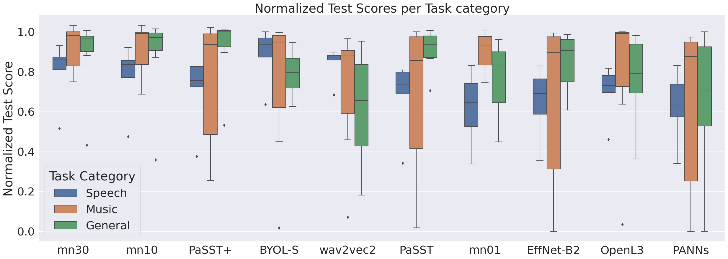
Figure 1: Comparing well-performing single models: PaSST and PaSST+ [15, 38] (supervised, Transformers), wav2vec2 [9] (self-supervised, Transformer), BYOL-S [39] and OpenL3 [6] (self-supervised, CNNs), and RedRice/Xiaomi EffNet-B2 [32] and PANNs CNN14 [21] (supervised, CNNs) to mn01, mn10 and mn30. We compare the distributions of normalized scores per task category between the models. The models are ordered according to the median value of the normalized scores across all tasks in descending order from left to right.

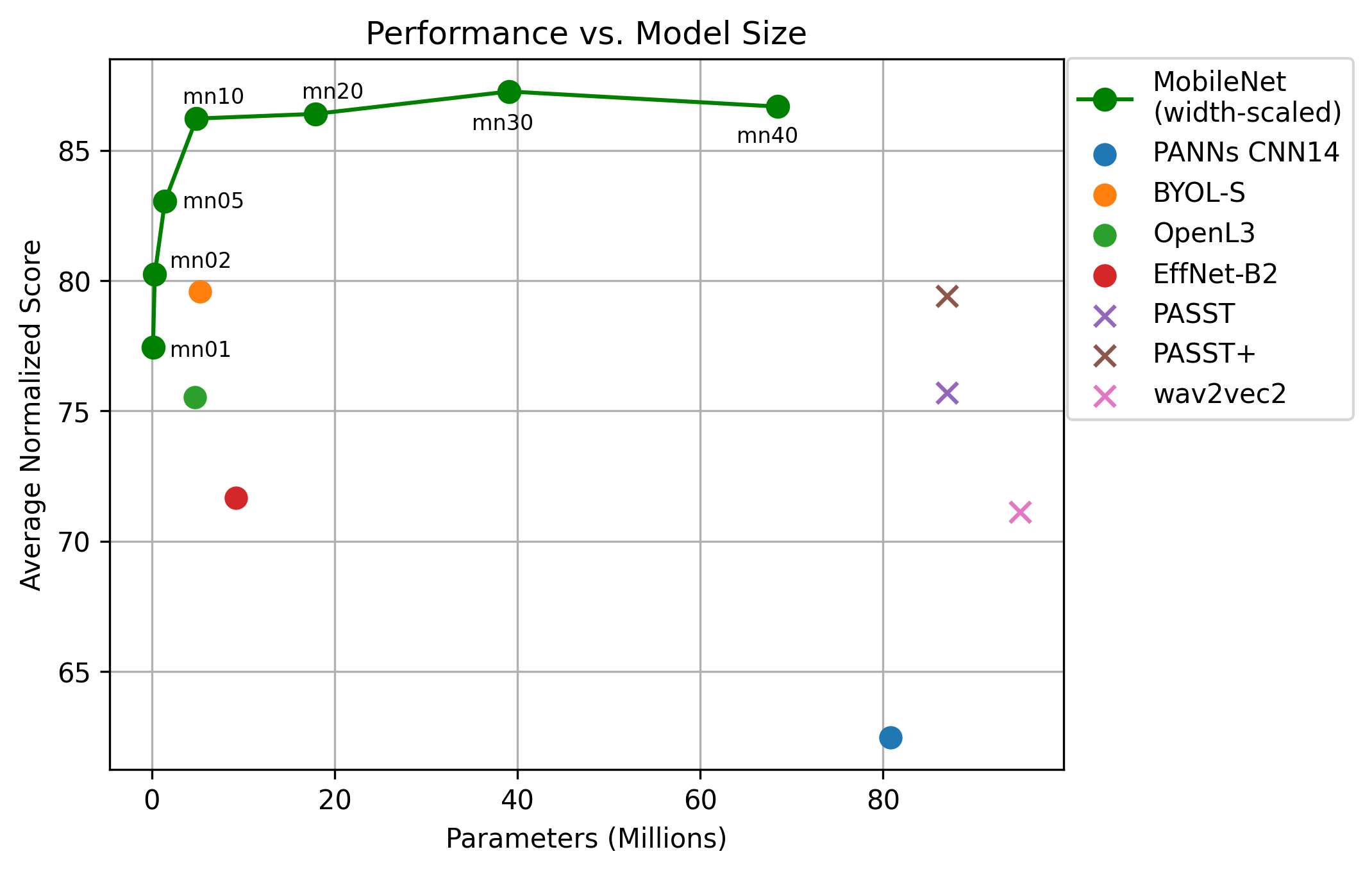
Figure 2: Comparing width-scaled ($\alpha\in\{0.1,0.2,0.5,1.0,2.0,3.0,4.0\}$) MobileNets to other well-performing single models with respect to the parameter-efficiency. Circles/Crosses denote CNNs/Transformers.

IV-B Low-complexity Audio Embedding Extraction

In this section, we scale our models by adapting the width scaling factor $\alpha$ and compare the performance of models ranging from 0.12M (mn01) to 68M parameters (mn40). For all models, we use the best-performing feature set (M_B+L) found in Section IV-A.

Parameter Complexity: Figure 2 compares the number of parameters against the average normalized scores of our width-scaled models ($\alpha\in\{0.1,0.2,0.5,1.0,2.0,3.0,4.0\}$) in comparison to well-performing single models submitted to the HEAR 21 challenge [1]. In addition, we include PaSST+ [38], an improved version of PaSST [15] that uses a smaller hop size and concatenates mel features with two receptive fields of different sizes for timestamp embeddings.

On the low-complexity end, our proposed models show an excellent parameter-performance trade-off. The smallest model mn01 performs worse than larger MobileNets and is outperformed by BYOL-S [39] (CNN trained in a self-supervised fashion) and PaSST+ [38] (Transformer trained on AudioSet [20] labels). However, with 120k parameters, it contains a fraction of the parameters of the other models and still provides audio embeddings of very competitive performance.

The performance of our models increases sharply until mn10 (4.88M parameters), with more complex models being only slightly better. mn30 reaches the highest performance, indicating that scaling up our models further is hitting a performance limit.

Computational Complexity: Complementary to the model size, the computational complexity at inference time specified in terms of multiply-accumulate (MAC) operations is an important factor for deploying models on resource-constrained devices. The computational demand of our models ranges from 20M (mn01) over 540M (mn10) up to 8B (mn40) MACs per 10 seconds of processed audio signal. In comparison to other models (PaSST: 128B, CNN14: 20B, EffNet-B2: 900M, Byol-S: 780M), our pre-trained MobileNets are computationally lightweight. For example, mn01 could run real-time inference on an embedded processor supporting single-cycle MAC and operating in low MHz range, such as a Cortex-M4.

IV-C Comparison to Single Models

Figure 1 compares mn01, mn10 and mn30 to other well-performing single models submitted to HEAR based on the normalized score distributions for the categories Speech, Music and General. In the Speech category, our models are outperformed by BYOL-S [39] and wav2vec2 [9], two models that are specialized in speech tasks. However, mn10 and mn30 outperform all models not pre-trained on speech datasets. The Music category is dominated by our models with mn01 exceeding the top challenge score on the task Beijing Opera Percussion (recognize the type of percussion instrument) and mn30 setting new top scores for the tasks Mridingham Tonic (classify tonics), Mridingham Stroke (classify strokes) and GTZAN Genre (classify genre). PaSST+ achieves the best results in the General category, closely followed by our models. mn10 sets a new top score on the task Vocal Imitations (retrieve sound using vocal imitation) and mn30 exceeds the top score on ESC-50 (environmental sound classification). Overall, mn30 and mn10 compare favorably against all other single models, being among the best models in each category. The tiny model mn01 performs comparable to EffNet-B2 [32], OpenL3 [6] and PANNs CNN14 [21], and slightly worse than PaSST [15].

V Conclusion

In this work, we used recently introduced highly efficient state-of-the-art audio tagging models [29] pre-trained on AudioSet [20] as low-complexity general-purpose audio embedding extractors. We tested which feature sets generalize best to a variety of downstream tasks and found that mid-level features perform best while adding low-level features brings in the necessary pitch information to master music-related tasks. Based on these findings, we varied the model complexity and showed that our scaled models are more parameter efficient and less computationally demanding than previously proposed models. We propose a tiny model mn01 that extracts audio embeddings of competitive quality for the application on edge devices. The larger mn10 is still very compact and compares favorably against other single models submitted to the HEAR challenge and, finally, the larger mn30 outperforms mn10 and beats the top HEAR challenge test scores on 4 tasks.

References

- [1] J. Turian, J. Shier, H. R. Khan, B. Raj, B. W. Schuller, C. J. Steinmetz, C. Malloy, G. Tzanetakis, G. Velarde, K. McNally, M. Henry, N. Pinto, C. Noufi, C. Clough, D. Herremans, E. Fonseca, J. H. Engel, J. Salamon, P. Esling, P. Manocha, S. Watanabe, Z. Jin, and Y. Bisk, “HEAR: holistic evaluation of audio representations,” in NeurIPS 2021 Competitions and Demonstrations Track. PMLR, 2021.
- [2] Z. Liu, Y. Wang, and T. Chen, “Audio feature extraction and analysis for scene segmentation and classification,” J. VLSI Signal Process., 1998.
- [3] F. Eyben, M. Wöllmer, and B. W. Schuller, “Opensmile: the munich versatile and fast open-source audio feature extractor,” in Proceedings of the 18th International Conference on Multimedia. ACM, 2010.
- [4] B. Logan, “Mel frequency cepstral coefficients for music modeling,” in ISMIR, 1st International Symposium on Music Information Retrieval, 2000.
- [5] S. Hershey, S. Chaudhuri, D. P. W. Ellis, J. F. Gemmeke, A. Jansen, R. C. Moore, M. Plakal, D. Platt, R. A. Saurous, B. Seybold, M. Slaney, R. J. Weiss, and K. W. Wilson, “CNN architectures for large-scale audio classification,” in IEEE International Conference on Acoustics, Speech and Signal Processing, ICASSP. IEEE, 2017.
- [6] J. Cramer, H. Wu, J. Salamon, and J. P. Bello, “Look, listen, and learn more: Design choices for deep audio embeddings,” in IEEE International Conference on Acoustics, Speech and Signal Processing, ICASSP. IEEE, 2019.
- [7] A. van den Oord, Y. Li, and O. Vinyals, “Representation learning with contrastive predictive coding,” CoRR, 2018.
- [8] D. Niizumi, D. Takeuchi, Y. Ohishi, N. Harada, and K. Kashino, “BYOL for audio: Self-supervised learning for general-purpose audio representation,” in International Joint Conference on Neural Networks, IJCNN. IEEE, 2021.
- [9] A. Baevski, Y. Zhou, A. Mohamed, and M. Auli, “wav2vec 2.0: A framework for self-supervised learning of speech representations,” in Annual Conference on Neural Information Processing Systems, NeurIPS, 2020.
- [10] A. van den Oord, S. Dieleman, H. Zen, K. Simonyan, O. Vinyals, A. Graves, N. Kalchbrenner, A. W. Senior, and K. Kavukcuoglu, “Wavenet: A generative model for raw audio,” in The 9th ISCA Speech Synthesis Workshop. ISCA, 2016.
- [11] S. Mehri, K. Kumar, I. Gulrajani, R. Kumar, S. Jain, J. Sotelo, A. C. Courville, and Y. Bengio, “Samplernn: An unconditional end-to-end neural audio generation model,” in 5th International Conference on Learning Representations, ICLR. OpenReview.net, 2017.
- [12] A. Dosovitskiy, L. Beyer, A. Kolesnikov, D. Weissenborn, X. Zhai, T. Unterthiner, M. Dehghani, M. Minderer, G. Heigold, S. Gelly, J. Uszkoreit, and N. Houlsby, “An image is worth 16x16 words: Transformers for image recognition at scale,” in 9th International Conference on Learning Representations, ICLR. OpenReview.net, 2021.
- [13] K. He, X. Chen, S. Xie, Y. Li, P. Dollár, and R. B. Girshick, “Masked autoencoders are scalable vision learners,” in IEEE/CVF Conference on Computer Vision and Pattern Recognition, CVPR. IEEE, 2022.
- [14] Y. Gong, Y. Chung, and J. R. Glass, “AST: audio spectrogram transformer,” in Interspeech, 22nd Annual Conference of the International Speech Communication Association. ISCA, 2021.
- [15] K. Koutini, J. Schlüter, H. Eghbal-zadeh, and G. Widmer, “Efficient training of audio transformers with patchout,” in Interspeech, 23rd Annual Conference of the International Speech Communication Association. ISCA, 2022.
- [16] D. Niizumi, D. Takeuchi, Y. Ohishi, N. Harada, and K. Kashino, “Masked spectrogram modeling using masked autoencoders for learning general-purpose audio representation,” CoRR, 2022.
- [17] D. Chong, H. Wang, P. Zhou, and Q. Zeng, “Masked spectrogram prediction for self-supervised audio pre-training,” CoRR, 2022.
- [18] A. Baade, P. Peng, and D. Harwath, “MAE-AST: masked autoencoding audio spectrogram transformer,” in Interspeech, 23rd Annual Conference of the International Speech. ISCA, 2022.
- [19] J. Deng, W. Dong, R. Socher, L. Li, K. Li, and L. Fei-Fei, “Imagenet: A large-scale hierarchical image database,” in IEEE Computer Society Conference on Computer Vision and Pattern Recognition, CVPR. IEEE Computer Society, 2009.
- [20] J. F. Gemmeke, D. P. W. Ellis, D. Freedman, A. Jansen, W. Lawrence, R. C. Moore, M. Plakal, and M. Ritter, “Audio set: An ontology and human-labeled dataset for audio events,” in IEEE International Conference on Acoustics, Speech and Signal Processing, ICASSP. IEEE, 2017.
- [21] Q. Kong, Y. Cao, T. Iqbal, Y. Wang, W. Wang, and M. D. Plumbley, “Panns: Large-scale pretrained audio neural networks for audio pattern recognition,” IEEE ACM Trans. Audio Speech Lang. Process., 2020.
- [22] P. Huang, H. Xu, J. Li, A. Baevski, M. Auli, W. Galuba, F. Metze, and C. Feichtenhofer, “Masked autoencoders that listen,” in Annual Conference on Neural Information Processing Systems, NeurIPS, 2022.
- [23] Y. Gong, C. Lai, Y. Chung, and J. R. Glass, “SSAST: self-supervised audio spectrogram transformer,” in Thirty-Sixth AAAI Conference on Artificial Intelligence. AAAI Press, 2022.
- [24] A. Saeed, D. Grangier, and N. Zeghidour, “Contrastive learning of general-purpose audio representations,” in IEEE International Conference on Acoustics, Speech and Signal Processing, ICASSP. IEEE, 2021.
- [25] L. Wang, P. Luc, Y. Wu, A. Recasens, L. Smaira, A. Brock, A. Jaegle, J. Alayrac, S. Dieleman, J. Carreira, and A. van den Oord, “Towards learning universal audio representations,” in IEEE International Conference on Acoustics, Speech and Signal Processing, ICASSP. IEEE, 2022.
- [26] M. Tagliasacchi, B. Gfeller, F. de Chaumont Quitry, and D. Roblek, “Self-supervised audio representation learning for mobile devices,” CoRR, 2019.
- [27] P. Lopez-Meyer, J. A. del Hoyo Ontiveros, H. Lu, and G. Stemmer, “Efficient end-to-end audio embeddings generation for audio classification on target applications,” in IEEE International Conference on Acoustics, Speech and Signal Processing, ICASSP. IEEE, 2021.
- [28] A. Howard, R. Pang, H. Adam, Q. V. Le, M. Sandler, B. Chen, W. Wang, L. Chen, M. Tan, G. Chu, V. Vasudevan, and Y. Zhu, “Searching for mobilenetv3,” in IEEE/CVF International Conference on Computer Vision, ICCV. IEEE, 2019.
- [29] F. Schmid, K. Koutini, and G. Widmer, “Efficient large-scale audio tagging via transformer-to-cnn knowledge distillation,” in IEEE International Conference on Acoustics, Speech and Signal Processing, ICASSP. IEEE, 2023.
- [30] A. G. Howard, M. Zhu, B. Chen, D. Kalenichenko, W. Wang, T. Weyand, M. Andreetto, and H. Adam, “Mobilenets: Efficient convolutional neural networks for mobile vision applications,” CoRR, 2017.
- [31] M. Sandler, A. G. Howard, M. Zhu, A. Zhmoginov, and L. Chen, “Mobilenetv2: Inverted residuals and linear bottlenecks,” in IEEE Conference on Computer Vision and Pattern Recognition, CVPR. Computer Vision Foundation / IEEE Computer Society, 2018.
- [32] M. Tan and Q. V. Le, “Efficientnet: Rethinking model scaling for convolutional neural networks,” in Proceedings of the 36th International Conference on Machine Learning, ICML. PMLR, 2019.
- [33] ——, “Efficientnetv2: Smaller models and faster training,” in Proceedings of the 38th International Conference on Machine Learning, ICML. PMLR, 2021.
- [34] Y. Gong, Y. Chung, and J. R. Glass, “PSLA: improving audio tagging with pretraining, sampling, labeling, and aggregation,” IEEE ACM Trans. Audio Speech Lang. Process., 2021.
- [35] Y. Gong, S. Khurana, A. Rouditchenko, and J. R. Glass, “CMKD: cnn/transformer-based cross-model knowledge distillation for audio classification,” CoRR, 2022.
- [36] J. Hu, L. Shen, and G. Sun, “Squeeze-and-excitation networks,” in IEEE Conference on Computer Vision and Pattern Recognition, CVPR. Computer Vision Foundation / IEEE Computer Society, 2018.
- [37] D. Niizumi, D. Takeuchi, Y. Ohishi, N. Harada, and K. Kashino, “Composing general audio representation by fusing multilayer features of a pre-trained model,” in 30th European Signal Processing Conference, EUSIPCO. IEEE, 2022.
- [38] K. Koutini, S. Masoudian, F. Schmid, H. Eghbal-zadeh, J. Schlüter, and G. Widmer, “Learning general audio representations with large-scale training of patchout audio transformers,” in HEAR. PMLR, 2023.
- [39] G. Elbanna, N. Scheidwasser-Clow, M. Kegler, P. Beckmann, K. E. Hajal, and M. Cernak, “BYOL-S: learning self-supervised speech representations by bootstrapping,” in HEAR. PMLR, 2023.