On the nonmonotone linesearch for a class of infinite-dimensional nonsmooth problems

Abstract

This paper provides a comprehensive study of the nonmonotone forward-backward splitting (FBS) method for solving a class of nonsmooth composite problems in Hilbert spaces. The objective function is the sum of a Fréchet differentiable (not necessarily convex) function and a proper lower semicontinuous convex (not necessarily smooth) function. These problems appear, for example, frequently in the context of optimal control of nonlinear partial differential equations (PDEs) with nonsmooth sparsity promoting cost functionals. We discuss the convergence and complexity of FBS equipped with the nonmonotone linesearch under different conditions. In particular, R-linear convergence will be derived under quadratic growth-type conditions. We also investigate the applicability of the algorithm to problems governed by PDEs. Numerical experiments are also given that justify our theoretical findings.

1 Introduction

In this work, we are concerned with the following composite problem

$$\min_{u\in{H}}\hskip 3.98337pt{\Psi}(u)\coloneqq{\mathcal{F}}(u)+{\mathcal{R}}(u),$$ (O)

where ${H}$ is a real Hilbert space, ${\mathcal{F}}$ is a continuously Fréchet differentiable function (possibly nonconvex), and ${\mathcal{R}}$ is a convex function whose proximal operator is assumed to be explicitly computable. The precise details will be introduced in Section 2. Problems of the form (O) appear in several fields of application such as optimal control problems AzmKunRod ; 6422363 , system identification , signal and image processing MR2858838 , machine learning, and statistics parikh2014proximal .

Arguably one of the most well-known algorithms for solving problem (O) is forward-backward splitting (FBS), also known as the proximal gradient method B17 ; MR2858838 , which is the generalization of the classical gradient method for problems with an additional nonsmooth term (see (8)). The iterations of FBS are defined by

$$u_{k+1}=\operatorname{Prox}_{\frac{1}{\alpha_{k}}{\mathcal{R}}}\left(u_{k}-\frac{1}{\alpha_{k}}{\nabla{\mathcal{F}}}(u_{k})\right), \text{for }k\in{\mathbb{N}}_{0},$$ (1)

where the step-sizes $\alpha_{k}>0$ are supposed to be choosen in a way that guarantees convergence of the algorithm and accelerates it. It is known that global convergence of FBS is to be sublinear of order $(1/k)$ for the convex case B17 , where $k$ stands for the number of iterations. This order can be improved to $(1/k^{2})$ using an inertial variant of the algorithm based on Nesterov’s accelerated techniques zbMATH05618078 ; zbMATH06197840 . Convergence of the iterates of FBS to a critical point of problem (O), even for the nonconvex case, has been shown for functions ${\Psi}$ satisfying the Kurdyka–Łojasiewicz property e.g., zbMATH05382665 ; zbMATH06145973 ; MR3707370 ; MR3341671 or quadratic growth error bounds e.g., MR4215308 ; DruLew_Error ; garrigos_convergence_2022 ; necoara_linear_2019 . Due to the simplicity and efficiency of FBS, the convergence, complexity, and applicability of this approach have been extensively studied in the literature, and it is still considered an active research area. Many different step-size strategies have been proposed and studied in the context of FBS under different assumptions. Among them, we mention MR4218411 ; MR3500980 ; MR3482398 ; MR3429743 ; MR3845278 for the finite-dimensional setting and MR3616647 ; MR4215308 ; MR4430995 ; MR3707899 for the infinite-dimensional setting.

As is well-known for smooth problems, the nonmonotone linesearch appears numerically efficient in situations where the monotone scheme is forced to propagate along the bottom of a narrow curved valley. Further, due to the fact that it permits growth in function values, it can be combined in an efficient manner with spectral gradient methods such as Barzilai-Borwein (BB) step-sizes azmi_analysis_2020 ; MR967848 , which inherently have a nonmonotone behavior. Based on the nonmonotone approach developed by Grippo et al MR849278 , Wright et al MR2650165 proposed a nonmontone FBS for convex composite optimization problem posed in $\mathbb{R}^{n}$. The convergence of this approach known as SparSa is further studied in MR2792408 and the order $(1/k)$ and R-linear convergence have been proven for convex and strongly convex functions, respectively. Very recently, in MR4504980 , the authors managed to prove convergence to a critical point of this scheme for a finite-dimensional nonconvex composite function under milder conditions, i.e., local Lipschitz continuity of the gradient for the smooth part and uniform continuity for the objective function on its level sets.

From a computational point of view, both classic gradient methods and FBS can be accelerated provided that they are combined with the BB step-sizes for approximating the curvature of the objective function and its smooth part, respectively. In particular, the BB step-sizes appear to be quite efficient in the context of PDE-constrained optimization. In case of a strongly quadratic smooth part, R-linear convergence is established in case of a sufficiently small spectral condition number $(\leq 2)$ of the quadratic operator, see (azmi_analysis_2020, , Remark 3.4). However, even in case of a quadratic smooth part with condition numbers larger than $2$, convergence of the BB step-sizes is not clear and, to guarantee it, one needs to combine the BB step-sizes with a nonmonotone linesearch, which is relying on function evaluations.

Weak and strong convergence can be distinguished only in the infinite-dimensional setting. In practice, a numerical solution of an infinite-dimensional problem is of course obtained by the numerical implementation of algorithms for finite-dimensional approximations of these problems. However, to ensure the numerical robustness and stability of the finite-dimensional approximations, it is of great interest to analyze the convergence properties of the algorithm in the infinite-dimensional setting. These are expressed by the so-called mesh-independent principle (MIP), see e.g., MR821912 ; Behzad2021 ; MR1202003 ; MR2085262 ; MR912453 ; MR1049770 ; MR1756894 . Roughly speaking, based on the infinite-dimensional convergence results, this principle gives predictions about the convergence properties of finite-dimensional approximations (discretized problems). MIP also provides a theoretical justification for the development of refinement strategies, see e.g., MR917455 .

In light of the above discussion, and despite the numerical efficiency of nonmonotone FBS for problems with PDEs, to the best of our knowledge this approach has not yet been studied for infinite-dimensional problems. In this paper, we take a step towards this direction and address convergence and complexity of the nonmonotone FBS for problem (O).

Contribution

More precisely, the contributions of this work can be summarized as follows: (i) Starting with the nonconvex case, we prove well-posedness of the algorithm even without Lipschitz continuity of the gradient of ${\mathcal{F}}$. Under the global Lipschitz continuity of the gradient of ${\mathcal{F}}$, we prove global convergence of the algorithm with complexity $(1/\sqrt{k})$. To be more precise, we show that the norm of the prox-gradient mapping of iterates vanishes with complexity $(1/\sqrt{k})$. (ii) We also establish that every weak sequential cluster point of iterates is a stationary point. (iii) We derive the worst-case evaluation complexity of finding an $\varepsilon_{\mathrm{tol}}$-stationary point. More precisely, we give estimates on the maximal number of function and prox-grad operator evaluations for computing an approximate stationary point with a user-defined accuracy threshold $\varepsilon_{\mathrm{tol}}>0$. (iv) In the convex setting, relying on the concept of quasi-Fejer sequences, we are able to extend previously established results to global convergence, both in terms of function values and iterates with respect to the sequential weak topology. Further, we show that the convergence is sublinear of order $(1/k)$ in function values. (v) Under quadratic growth-type conditions, we show global R-linear convergence, both in terms of function values and iterates. The proof of the latter is more delicate for infinite-dimensional problems since the transition from weak sequential convergence to strong convergence is not straightforward. (vi) Finally, aiming at optimization problems governed by PDEs, we discuss the validity of the convergence results of the algorithm without strong Lipschitz continuity of ${\nabla{\mathcal{F}}}$. Our theoretical framework is supported by two nonsmooth problems governed by PDEs, including semilinear elliptic and parabolic equations. Finally, we show that our results are applicable to these problems and report on numerical findings.

Outline of the paper

The rest of this paper is organized as follows: Section 2 presents the preliminaries, assumptions on the optimization problem (O), the algorithm, and the nonmonotone linesearch strategy. Section 3 investigates the convergence and complexity of the algorithm comprehensively under different conditions. Section 4 discusses the applicability of the results from the previous section to PDE-constrained optimization problems. Finally, numerical experiments are reported in Section 5 that justify our theoretical findings. To improve the readability of the paper, we provide proofs to some results from Section 3 in Appendix A.

Notation

Throughout this paper, the Hilbert space ${H}$ is endowed with the scalar product $(\cdot,\cdot)_{H}$ and the induced norm $\|\cdot\|_{H}$. For a radius $r>0$ and $\bar{u}\in{H}$, we define $\mathbf{B}_{r}(\bar{u}):=\{u\in{H}:\|u-\bar{u}\|_{{H}}<r\}$. We also denote with $P_{S}:{H}\to{H}$, the orthogonal projection onto the set $S\subset{H}$. Further for every $\tilde{{\Psi}}\in\mathbb{R}$, we define $\left[{\Psi}\leq\tilde{{\Psi}}\right]:=\{u\in{H}:{\Psi}(u)\leq\tilde{{\Psi}}\}$. By $\operatorname{Argmin}{\Psi}$ we denote the set of minimizers of ${\Psi}$. Sometimes we will use set-values (in-)equalities, i.e. $A\leq B$ for $A,B\subset{H}$, meaning that $a\leq b$ for all $a\in A$ and $b\in B$.

We call a sequence $\{u_{k}\}_{k}\subset{H}$ quasi-Féjer monotone with respect to a non-empty set $S\subset{H}$, if for every $v\in S$ it holds that

$$\|u_{k+1}-v\|^{2}_{{H}}\leq\|u_{k}-v\|^{2}_{{H}}+\epsilon_{k},$$

where $\{\epsilon_{k}\}_{k}\subset\mathbb{R}_{\geq 0}$ is a summable sequence, i.e., $\sum^{\infty}_{k=0}\epsilon_{k}<\infty$. To avoid confusion in the notation, the derivative and gradient of ${\mathcal{F}}$ are defined by ${\mathcal{F}}^{\prime}\colon{H}\rightarrow{H}^{\prime}$ and $\nabla{\mathcal{F}}\colon{H}\rightarrow{H}$, respectively. In this case, for every $u\in{H}$ we identify $\nabla{\mathcal{F}}(u)\in{H}$ with the unique Riesz representative of ${\mathcal{F}}^{\prime}\in{H}^{\prime}$.

2 Problem formulation and algorithm

In this section the precise theoretical framework and algorithm will be introduced. First, we review some notions of stationarity for nonconvex and nonsmooth functions. The Fréchet subdifferential of $\phi:{H}\to{\mathbb{R}}\cup\{\pm\infty\}$ at $u\in\operatorname{dom}\phi$ is defined as

$$\hat{\partial}\phi(u):=\left\{w\in{H}:\liminf_{v\to u}\frac{\phi(v)-\phi(u)-(w,v-u)_{H}}{\|v-u\|_{H}}\geq 0\right\}.$$

For this notion of subdifferential, we obtain the Fermat principle (zbMATH05162727, , Proposition 9.1.5) for the local minimizers stating the following.

Proposition 1

Let $\phi:{H}\to{\mathbb{R}}\cup\{\pm\infty\}$ be proper and lower semicontinuous and $u^{*}\in\operatorname{dom}\phi$ be a local minimizer. Then $0\in\hat{\partial}\phi(u^{*})$.

The Fréchet subdifferential fails to be outer semicontinuous, which is also not desirable. To mitigate this issue, we mention the Mordukhovich or limiting subdifferential of $\phi$ at $u\in\operatorname{dom}\phi$, which is defined as the sequential Painlevé-Kuratowski outer limit of $\hat{\partial}\phi(u)$ (zbMATH02176481, , Theorem 2.34), that is

$$\partial_{M}\phi(u):=\left\{w\in{H}:\exists\{u_{n}\}_{n},\{w_{n}\}_{n}\subset{H}\text{ s.t. }u_{n}\xrightarrow{\phi}u,w_{n}\rightharpoonup w\text{ with }w_{n}\in\hat{\partial}\phi(u_{n})\right\}.$$

Here $u_{n}\xrightarrow{\phi}u$ stands for $u_{n}\to u$ with $\phi(u_{n})\to\phi(u)$. We can infer directly from the definition that $\hat{\partial}\phi(u)\subset\partial_{M}\phi(u)$. Here, we summarize from zbMATH02176481 , some of the results for these subdifferentials

• If $\phi$ is convex, the above notions of subdifferential coincide with the convex subdifferential. That is $\hat{\partial}\phi(u)=\partial_{M}\phi(u)=\partial\phi(u)$ with $\partial\phi(u):=\{w\in{H}:\phi(v)-\phi(u)\geq(w,v-u)_{H}\text{ for all }v\in{H}\}$.

• For every continuously Fréchet differentiable function $\phi$, the above notions of subdifferential reduce to the first derivative, i.e. $\hat{\partial}\phi(u)=\partial_{M}\phi(u)=\{\nabla\phi(u)\}$.

• Given an arbitrary function $\psi:{H}\to{\mathbb{R}}\cup\{\pm\infty\}$, which is finite at $u$ and a function $\phi:{H}\to{\mathbb{R}}\cup\{\pm\infty\}$, that is continuously Fréchet differentiable at $u$, we have

  $$\hat{\partial}(\phi+\psi)(u)=\nabla\phi(u)+\hat{\partial}\psi(u)\text{ and }\partial_{M}(\phi+\psi)(u)=\nabla\phi(u)+\partial_{M}\psi(u).$$ (2)

Therefore, according to Assumption 1 and Proposition (1), the Fermat principle for (O) reads as follows: If $u^{*}\in{H}$ is a local minimizer of ${\Psi}$, then

$$-{\nabla{\mathcal{F}}}(u^{*})\in\partial{\mathcal{R}}(u^{*}),$$ (3)

and, with similar arguments as in the proof (MR3616647, , Theorem 26.2), (3) can be equivalently expressed as

$$u^{*}=\operatorname{Prox}_{\frac{1}{{\alpha}}{\mathcal{R}}}(u^{*}-\frac{1}{{\alpha}}{\nabla{\mathcal{F}}}(u^{*}))\quad\text{ for some }{\alpha}>0.$$ (4)

where the proximal operator $\operatorname{Prox}_{\frac{1}{{\alpha}}{\mathcal{R}}}:{H}\to{H}$ is defined by

$$\operatorname{Prox}_{\frac{1}{{\alpha}}{\mathcal{R}}}(u):=\arg\!\min_{v\in{H}}\left({\mathcal{R}}(v)+\frac{{\alpha}}{2}\|v-u\|_{H}^{2}\right).$$

This operator is well-defined provided that ${\mathcal{R}}$ is proper, convex, and lower semicontinuous. We also define the set of critical points by

$${S_{*}}:=\{u\in{H}:-{\nabla{\mathcal{F}}}(u)\in\partial{\mathcal{R}}(u)\}.$$

Now we are in the position that we can state the precise assumptions on (O).

For problem (O),

A1:

${\mathcal{R}}\colon{H}\rightarrow{\mathbb{R}}\cup\{\pm\infty\}$ is proper, convex, and lower semicontinuous.

A2:

${\mathcal{F}}\colon{H}\rightarrow{\mathbb{R}}$ is continuously Fréchet differentiable on ${\operatorname{int}(\operatorname{dom}{\mathcal{F}})}$ containing $\operatorname{dom}{\mathcal{R}}$, that is, $\operatorname{dom}{\mathcal{R}}\subseteq{\operatorname{int}(\operatorname{dom}{\mathcal{F}})}$.

A3:

${\nabla{\mathcal{F}}}\colon{H}\rightarrow{H}$ is globally ${L_{{\mathcal{F}}^{\prime}}}$-Lipschitz continuous.

A4:

The gradient ${\nabla{\mathcal{F}}}\colon{\operatorname{int}(\operatorname{dom}{\mathcal{F}})}\rightarrow{H}$ is weak-to-strong sequentially continuous.

Conditions A1:-A2: are standard in order to guarantee the well-posedness of the algorithm. A3: will be used to derive complexity results for iterations and we will discuss the relaxation of this condition for a large class of problems governed by PDEs. We use A4: to show that every weak sequential accumulation point of iterates belongs to the set ${S_{*}}$. Note that, if $\dim({H})<\infty$, A4: follows from A2:.

Now we turn our attention towards formalizing (1) and the proposed step-size update strategy by a nonmonotone linesearch method. Therefore we introduce the prox-grad operator and the gradient mapping analogously to B17 ; DruLew_Error in the Hilbert space setting.

Definition 1

For every $\alpha\in\mathbb{R}_{>0}$, we define

1. the prox-grad operator ${\mathcal{T}}_{\alpha}\colon{\operatorname{int}(\operatorname{dom}{\mathcal{F}})}\rightarrow\operatorname{dom}{\mathcal{R}}$ with $u\mapsto\operatorname{Prox}_{\frac{1}{{\alpha}}{\mathcal{R}}}(u-\frac{1}{{\alpha}}{\nabla{\mathcal{F}}}(u))$.

2. the gradient mapping ${\mathcal{G}}_{\alpha}\colon{\operatorname{int}(\operatorname{dom}{\mathcal{F}})}\rightarrow{H}$ with $u\mapsto{\alpha}(u-{\mathcal{T}}_{\alpha}(u))$.

Due to Definition 1 and by some simple computations, we obtain for every $u\in{\operatorname{int}(\operatorname{dom}{\mathcal{F}})}$ that

$${\mathcal{G}}_{\alpha}(u)-{\nabla{\mathcal{F}}}(u)\in\partial{\mathcal{R}}({\mathcal{T}}_{\alpha}(u)).$$ (5)

Further, if we define for every $u\in{\operatorname{int}(\operatorname{dom}{\mathcal{F}})}$, $w\in{H}$, and ${\alpha}\in\mathbb{R}_{>0}$

$$\mathcal{Q}_{{\alpha}}(w,u):={\mathcal{F}}(u)+({\nabla{\mathcal{F}}}(u),w-u)_{H}+\frac{{\alpha}}{2}\|w-u\|_{H}^{2}+{\mathcal{R}}(w),$$

then ${\mathcal{T}}_{{\alpha}}(u)$ is the unique minimizer of $\mathcal{Q}_{{\alpha}}(\cdot,u)$, i.e.

$${\mathcal{T}}_{{\alpha}}(u)=\arg\!\min_{w\in{H}}\mathcal{Q}_{{\alpha}}(w,u).$$

As a consequence, we can write

$$({\nabla{\mathcal{F}}}(u),{\mathcal{T}}_{{\alpha}}(u)-u)_{H}+\frac{1}{2{\alpha}}\|{\mathcal{G}}_{\alpha}(u)\|_{H}^{2}+{\mathcal{R}}({\mathcal{T}}_{{\alpha}}(u))\leq{\mathcal{R}}(u).$$ (6)

By means of the prox-grad operator and the gradient mapping (1) can be reformulated as follows:

$$u_{k+1} ={\mathcal{T}}_{\alpha_{k}}(u_{k}), \text{for }k\in{\mathbb{N}}_{0},$$ (7)

$$u_{k+1} =u_{k}-\frac{1}{\alpha_{k}}{\mathcal{G}}_{\alpha_{k}}(u_{k}), \text{for }k\in{\mathbb{N}}_{0}.$$ (8)

In this case, for every $u_{0}\in{\operatorname{int}(\operatorname{dom}{\mathcal{F}})}$, the iterations are well-defined, that is $\{u_{k}\}_{k}\subset\operatorname{dom}{\mathcal{R}}\subseteq{H}$. Further, due to (8) we can see the analogy between the proximal gradient method and classical gradient descent for smooth minimization. We also can characterize the critical points of (O), using the notion of the gradient mapping and (4) as follows.

Proposition 2

For $u^{*}\in{\operatorname{int}(\operatorname{dom}{\mathcal{F}})}$, it holds that ${\mathcal{G}}_{\alpha}(u^{*})=0$ for some ${\alpha}\in\mathbb{R}_{>0}$ if and only if $u^{*}\in{S_{*}}$.

Therefore ${\mathcal{G}}_{\alpha}({\bar{u}})=0$ defines a natural termination condition analogously to the smooth case.

There are many possible choices for the step-size $\alpha_{k}$ in our iterative scheme. In this work we will consider step-size updates by a BB-type update rule or a combination of them with a nonmonotone linesearch. To be more precise, as the first trial step-size within the nonmonotone linesearch, we will choose one of the spectral gradient BB-types step-sizes defined by

$$\alpha^{\mathrm{BB}1\mathrm{a}}_{k} \coloneqq\frac{{(u_{k}-u_{k-1},{\nabla{\mathcal{F}}}(u_{k})-{\nabla{\mathcal{F}}}(u_{k-1}))}_{H}}{{(u_{k}-u_{k-1},u_{k}-u_{k-1})}_{H}},$$

$$\alpha^{\mathrm{BB}2\mathrm{a}}_{k} \coloneqq\frac{{({\nabla{\mathcal{F}}}(u_{k})-{\nabla{\mathcal{F}}}(u_{k-1}),{\nabla{\mathcal{F}}}(u_{k})-{\nabla{\mathcal{F}}}(u_{k-1}))}_{H}}{{(u_{k}-u_{k-1},{\nabla{\mathcal{F}}}(u_{k})-{\nabla{\mathcal{F}}}(u_{k-1})}_{H}},$$

$$\alpha^{\mathrm{BB}1\mathrm{b}}_{k} \coloneqq\frac{{(u_{k}-u_{k-1},{\mathcal{G}}_{{\alpha}_{k-1}}(u_{k})-{\mathcal{G}}_{{\alpha}_{k-1}}(u_{k-1}))}_{H}}{{(u_{k}-u_{k-1},u_{k}-u_{k-1})}_{H}},$$

$$\alpha^{\mathrm{BB}2\mathrm{b}}_{k} \coloneqq\frac{{({\mathcal{G}}_{{\alpha}_{k-1}}(u_{k})-{\mathcal{G}}_{{\alpha}_{k-1}}(u_{k-1}),{\mathcal{G}}_{{\alpha}_{k-1}}(u_{k})-{\mathcal{G}}_{{\alpha}_{k-1}}(u_{k-1}))}_{H}}{{(u_{k}-u_{k-1},{\mathcal{G}}_{{\alpha}_{k-1}}(u_{k})-{\mathcal{G}}_{{\alpha}_{k-1}}(u_{k-1})}_{H}}.$$

The first two strategies correspond to the BB-method presented e.g. in Behzad2021 . The last two novel BB-methods modify the classical BB-method and try to incorporate full first order information by using the gradient mapping and not only the gradient of ${\mathcal{F}}$. Furthermore we will use so called alternating BB-type update rules given by

$$\alpha^{\mathrm{ABBa}} \coloneqq\alpha^{\mathrm{BB}1\mathrm{a}}\text{ for }k\text{ even and }\alpha^{\mathrm{BB}2\mathrm{a}}\text{ for }k\text{ odd},$$

$$\alpha^{\mathrm{ABBb}} \coloneqq\alpha^{\mathrm{BB}1\mathrm{b}}\text{ for }k\text{ even and }\alpha^{\mathrm{BB}2\mathrm{b}}\text{ for }k\text{ odd}.$$

Remark 1

In the case of ${\mathcal{R}}=0$ , we have ${\mathcal{G}}_{l}(u)={\nabla{\mathcal{F}}}(u)$ for every $l>0$ and $u\in H$. Therefore, many of the introduced step-size updates above are identical, i.e. $\alpha^{\mathrm{BB}1\mathrm{b}}=\alpha^{\mathrm{BB}1\mathrm{a}},\alpha^{\mathrm{BB}2\mathrm{b}}=\alpha^{\mathrm{BB}2\mathrm{a}}$ and $\alpha^{\mathrm{ABBb}}=\alpha^{\mathrm{ABBa}}$.

For the nonmonotone linesearch update, we choose

$${\Psi}(u_{k+1})\leq\max\limits_{0\leq j\leq m(k)}{\Psi}(u_{k-j})-\frac{\delta}{\alpha_{k}}\|{\mathcal{G}}_{\alpha_{k}}(u_{k})\|_{H}^{2},$$ (9)

with $0<\delta<1$ and memory $m\colon{\mathbb{N}}_{0}\rightarrow{\mathbb{N}}_{0}$ satisfying

$$m(0)=0, m(k)=\min\{m(k-1)+1,{m_{\mathrm{max}}}\} \text{for }k\in{\mathbb{N}},$$ (10)

with upper bound ${m_{\mathrm{max}}}\in{\mathbb{N}}_{0}$. Similarly to MR1915930 , we also define the functions $\ell:\mathbb{N}_{0}\to\mathbb{N}_{0}$ and $\nu:\mathbb{N}_{0}\to\mathbb{N}_{0}$ with

$$\ell(k) :=k-\arg\!\max\limits_{0\leq j\leq m(k)}{\Psi}(u_{k-j})\quad\text{ for }k\geq 0,\text{ with }k-m(k)\leq\ell(k)\leq k,$$

$$\nu(k) :=\ell(k{m_{\mathrm{max}}}+k),\quad\text{ for }k\geq 0.$$

Thus, by these notations, we have $\max\limits_{0\leq j\leq m(k)}{\Psi}(u_{k-j})={\Psi}(u_{\ell(k)})$ and (9) can be rewritten as

$${\Psi}(u_{k+1})\leq{\Psi}(u_{\ell(k)})-\frac{\delta}{\alpha_{k}}\|{\mathcal{G}}_{\alpha_{k}}(u_{k})\|_{H}^{2}.$$ (11)

Further we set

$$\alpha_{k}={\alpha_{\mathrm{int},k}}\eta^{i_{k}},$$ (12)

where $\eta>1$. The initial step-size ${\alpha_{\mathrm{int},k}}>0$ is chosen by the BB-method and a lower bound ${\alpha}_{\inf}>0$ is given to ensure nonnegativity. To limit the initial step-size numerically, also an upper bound ${\alpha}_{\sup}>{\alpha}_{\inf}$ is employed. In the update we choose the smallest integer $i_{k}\in{\mathbb{N}}_{0}$ in (12), such that (9) is satisfied. This procedure is summarized in Algorithm 1.

Require :  $0<\delta<1$, ${m_{\mathrm{max}}}\in\mathbb{N}_{0}$, $\eta>1$, ${\alpha}_{\sup}>{\alpha}_{\inf}>0$, $u_{0}\in{H}$ and ${\alpha}_{0}>0$

Return : Approximation $u^{*}\in{H}$ of stationary point of (O)

1 Set $k=0$ ;

2 while $\|{\mathcal{G}}_{\alpha_{k}}(u_{k})\|_{H}>0$ do

3       Compute $\alpha^{\mathrm{BB}}_{k}$ according to a BB-method and set ${\alpha_{\mathrm{int},k}}:=\max\{{\alpha}_{\inf},\min\{{\alpha}_{\sup},\alpha^{\mathrm{BB}}_{k}\}\}$;

4       Set $\alpha_{k}={\alpha_{\mathrm{int},k}}\eta^{i_{k}}$, where $i_{k}\geq 0$ is the smallest integer for which (9) holds ;

5       Set $u_{k+1}=u_{k}-\frac{1}{\alpha_{k}}{\mathcal{G}}_{\alpha_{k}}(u_{k})$ and $k=k+1$ ;

6      

Algorithm 1 Nonmonotone Splitting Algorithm

Note that by Proposition 2 the criterion $\|{\mathcal{G}}_{\alpha_{k}}(u_{k})\|_{H}\leq\varepsilon_{\mathrm{tol}}$ with some tolerance $\varepsilon_{\mathrm{tol}}>0$ is a reasonable stopping criterion in the numerical realization of Algorithm 1.

3 Convergence and complexity analysis

In this main section of our work, we present a detailed convergence and complexity analysis for Algorithm 1 under different assumptions and conditions.

3.1 General case

We start by summarizing useful properties of the gradient mapping.

Lemma 1

Suppose that A1:-A2: hold, then we have the following properties:

P1:

For every $l_{1}\geq l_{2}>0$ and $u\in{\operatorname{int}(\operatorname{dom}{\mathcal{F}})}$ it holds that $\frac{1}{l_{1}}\|{\mathcal{G}}_{l_{1}}(u)\|_{H}\leq\frac{1}{l_{2}}\|{\mathcal{G}}_{l_{2}}(u)\|_{H}$.

P2:

For every $l_{1}\geq l_{2}>0$ and $u\in{\operatorname{int}(\operatorname{dom}{\mathcal{F}})}$ it holds that $\|{\mathcal{G}}_{l_{1}}(u)\|_{H}\geq\|{\mathcal{G}}_{l_{2}}(u)\|_{H}$.

P3:

Assume in addition that A3: holds, then the gradient mapping is Lipschitz continuous, that is

$$\|{\mathcal{G}}_{l}(u)-{\mathcal{G}}_{l}(v)\|_{H}\leq(2l+{L_{{\mathcal{F}}^{\prime}}})\|u-v\|_{H},$$

for every $l>0$ and $v,u\in{\operatorname{int}(\operatorname{dom}{\mathcal{F}})}$.

Proof

The proof follows by similar arguments as e.g. given in (B17, , Theorem 10.9, Lemma 10.10) for finite-dimensional problems.

Furthermore the well-known sufficient decrease condition can be formulated with respect to the gradient mapping analogously to the finite-dimensional case presented in (B17, , Lemma 10.4).

Lemma 2 (Sufficient Decrease Lemma)

Suppose that A1:-A3: hold, then for every $u\in{\operatorname{int}(\operatorname{dom}{\mathcal{F}})}$ and $l\in(\frac{{L_{{\mathcal{F}}^{\prime}}}}{2},\infty)$, we have

$${\Psi}({\mathcal{T}}_{l}(u))\leq{\Psi}(u)-\frac{l-\frac{{L_{{\mathcal{F}}^{\prime}}}}{2}}{l^{2}}\|{\mathcal{G}}_{l}(u)\|_{H}^{2}.$$

The previous lemmas allow us to summarize some important properties of Algorithm 1.

Lemma 3

Suppose that A1:-A2: hold. Then for every $k\geq 0$, the following statements hold true:

1. For $\delta\in(0,\frac{1}{2})$, the nonmonotone linesearch is well-defined. That is, there exists $\underline{\alpha}>0$ such that for every $u_{k}\in{\operatorname{int}(\operatorname{dom}{\mathcal{F}})}$ and $\alpha_{k}\in[\underline{\alpha},\infty)$ the nonmonotone rule (9) holds and thus, the nonmonotone linesearch terminates after finitely many iterations.

Assume, in addition, A3: holds.

1. Then the statement of (i) is true for $\underline{\alpha}\coloneqq\frac{{L_{{\mathcal{F}}^{\prime}}}}{2(1-\delta)}$ and every fixed $\delta\in(0,1)$.

2. The step-sizes are uniformly bounded from above. That is, for every $k\geq 1$, we have $\alpha_{k}\leq\overline{{\alpha}}$ with $\overline{{\alpha}}\coloneqq\max\{\frac{\eta{L_{{\mathcal{F}}^{\prime}}}}{2(1-\delta)},{\alpha}_{\sup}\}$.

3. It holds $\|{\mathcal{G}}_{{\alpha}_{k+1}}(u_{k+1})\|_{H}\leq C_{G}\|{\mathcal{G}}_{\alpha_{k}}(u_{k})\|_{H}$, where $C_{G}:=\frac{3\overline{{\alpha}}+{L_{{\mathcal{F}}^{\prime}}}}{{\alpha}_{\inf}}$.

Proof

(i) If $u_{k}\in{S_{*}}$, then the claim clearly holds true for every $\underline{\alpha}>0$. Thus, we assume that $u_{k}\notin{S_{*}}$. We suppose also on contrary it does not exist $\underline{\alpha}>0$ for which the claim holds true. Then the nonmonote linesearch generates a sequence of step-sizes ${\alpha}_{k_{i}}:={\alpha_{\mathrm{int},k}}\eta^{i}$ with $i\in{\mathbb{N}}_{0}$ satisfying ${\alpha}_{k_{i}}\to\infty$ and

$$\frac{\delta}{{\alpha}_{k_{i}}}\|{\mathcal{G}}_{{\alpha}_{k_{i}}}(u_{k})\|_{H}^{2}>{\Psi}(u_{\ell(k)})-{\Psi}({\mathcal{T}}_{{\alpha}_{k_{i}}}(u_{k}))\geq{\Psi}(u_{k})-{\Psi}({\mathcal{T}}_{{\alpha}_{k_{i}}}(u_{k})).$$ (13)

First, we note that ${\mathcal{T}}_{{\alpha}_{k_{i}}}(u_{k})\to u_{k}$ as $i\to\infty$. This follows from the fact that $\operatorname{Prox}_{\frac{1}{{\alpha}_{k_{i}}}{\mathcal{R}}}(u_{k})\to u_{k}$ as $i\to\infty$ (see e.g., (MR3616647, , Theorem 23.47)) and

$$\begin{split}\|{\mathcal{T}}_{{\alpha}_{k_{i}}}(u_{k})-u_{k}\|_{H}&\leq\|\operatorname{Prox}_{\frac{1}{{\alpha}_{k_{i}}}{\mathcal{R}}}(u_{k}-\frac{1}{{\alpha}_{k_{i}}}{\nabla{\mathcal{F}}}(u_{k}))-\operatorname{Prox}_{\frac{1}{{\alpha}_{k_{i}}}{\mathcal{R}}}(u_{k})\|_{H}\\ &+\|\operatorname{Prox}_{\frac{1}{{\alpha}_{k_{i}}}{\mathcal{R}}}(u_{k})-u_{k}\|_{H}\leq\|\operatorname{Prox}_{\frac{1}{{\alpha}_{k_{i}}}{\mathcal{R}}}(u_{k})-u_{k}\|_{H}+\frac{1}{{\alpha}_{k_{i}}}\|{\nabla{\mathcal{F}}}(u_{k})\|_{H},\end{split}$$

where we have used the firm nonexpansiveness of the proximal operator. Further, using (13) and the mean value theorem for ${\mathcal{F}}$, we obtain for every $i\in{\mathbb{N}}_{0}$, that

$$\begin{split}&\frac{\delta}{{\alpha}_{k_{i}}}\|{\mathcal{G}}_{{\alpha}_{k_{i}}}(u_{k})\|_{H}^{2}\geq{\Psi}(u_{k})-{\Psi}({\mathcal{T}}_{{\alpha}_{k_{i}}}(u_{k}))\\ &\geq{\mathcal{R}}(u_{k})-{\mathcal{R}}({\mathcal{T}}_{{\alpha}_{k_{i}}}(u_{k}))+{({\nabla{\mathcal{F}}}(u_{k}+t_{i}({\mathcal{T}}_{{\alpha}_{k_{i}}}(u_{k}))-u_{k})),u_{k}-{\mathcal{T}}_{{\alpha}_{k_{i}}}(u_{k})))}_{H},\end{split}$$

where $t_{i}\in(0,1]$ for all $i\in{\mathbb{N}}_{0}$. Using (6) we obtain that

$$\begin{split}&\frac{\delta}{{\alpha}_{k_{i}}}\|{\mathcal{G}}_{{\alpha}_{k_{i}}}(u_{k})\|_{H}^{2}\geq\frac{1}{2{\alpha}_{k_{i}}}\|{\mathcal{G}}_{{\alpha}_{k_{i}}}(u_{k})\|_{H}^{2}\\ &+\left({\nabla{\mathcal{F}}}\left(u_{k}+t_{i}({\mathcal{T}}_{{\alpha}_{k_{i}}}(u_{k})-u_{k})\right)-{\nabla{\mathcal{F}}}(u_{k}),{\mathcal{T}}_{{\alpha}_{k_{i}}}(u_{k})-u_{k}\right)_{H}\\ &\geq\frac{1}{2{\alpha}_{k_{i}}}\|{\mathcal{G}}_{{\alpha}_{k_{i}}}(u_{k})\|_{H}^{2}\\ &-\frac{1}{{\alpha}_{k_{i}}}\|{\nabla{\mathcal{F}}}\left(u_{k}+t_{i}({\mathcal{T}}_{{\alpha}_{k_{i}}}(u_{k})-u_{k})\right)-{\nabla{\mathcal{F}}}(u_{k})\|_{H}\|{\mathcal{G}}_{{\alpha}_{k_{i}}}(u_{k})\|_{H}.\end{split}$$

Together with the fact that $\delta<\frac{1}{2}$ we obtain

$$(\frac{1}{2}-\delta)\|{\mathcal{G}}_{{\alpha}_{k_{i}}}(u_{k})\|_{H}\leq\|{\nabla{\mathcal{F}}}\left(u_{k}+t_{i}({\mathcal{T}}_{{\alpha}_{k_{i}}}(u_{k})-u_{k})\right)-{\nabla{\mathcal{F}}}(u_{k})\|_{H}.$$

Sending $i\to\infty$ and using the continuity of ${\nabla{\mathcal{F}}}$, we obtain that

$$\lim_{i\to\infty}\|{\mathcal{G}}_{{\alpha}_{k_{i}}}(u_{k})\|_{H}=0.$$

Finally, using P2:, we can infer that $\|{\mathcal{G}}_{{\alpha}_{\inf}}(u_{k})\|_{H}\leq\|{\mathcal{G}}_{{\alpha}_{k_{i}}}(u_{k})\|_{H}$ and thus $\|{\mathcal{G}}_{{\alpha}_{\inf}}(u_{k})\|_{H}=0$. Now Proposition 2 implies $u_{k}\in{S_{*}}$. This contradicts our assumption, which concludes the proof.

(ii) For every given $\alpha_{k}\geq\underline{\alpha}>\frac{{L_{{\mathcal{F}}^{\prime}}}}{2}$ we can invoke Lemma 2 and write

$$\begin{split}{\Psi}({\mathcal{T}}_{\alpha_{k}}(u_{k}))&\leq{\Psi}(u_{k})-\frac{\alpha_{k}-\frac{{L_{{\mathcal{F}}^{\prime}}}}{2}}{\alpha_{k}^{2}}\|{\mathcal{G}}_{\alpha_{k}}(u_{k})\|_{H}^{2}\\ \ &\leq\max\limits_{0\leq j\leq m(k)}{\Psi}(u_{k-j})-\frac{\alpha_{k}-\frac{{L_{{\mathcal{F}}^{\prime}}}}{2}}{\alpha_{k}^{2}}\|{\mathcal{G}}_{\alpha_{k}}(u_{k})\|_{H}^{2}.\end{split}$$

Thus, (9) holds since $\alpha_{k}$ satisfies $\frac{\alpha_{k}-\frac{{L_{{\mathcal{F}}^{\prime}}}}{2}}{\alpha_{k}^{2}}\geq\frac{\delta}{\alpha_{k}}$ by assumption.

(iii) To derive $\overline{{\alpha}}$, we consider the following cases:

• $i_{k}=0$: In this case, due to (12), we have $\alpha_{k}={\alpha_{\mathrm{int},k}}\leq{\alpha}_{\sup}$.

• $i_{k}\geq 1$: In this case, (9) holds for $\alpha_{k}$ and $u_{k}$. Then due to (12), we can write

  $$\begin{split}{\Psi}({\mathcal{T}}_{\frac{\alpha_{k}}{\eta}}(u_{k}))&>\max\limits_{0\leq j\leq m(k)}{\Psi}(u_{k-j})-\frac{\delta\eta}{\alpha_{k}}\|{\mathcal{G}}_{\frac{\alpha_{k}}{\eta}}(u_{k})\|_{H}^{2}\\ &\geq{\Psi}(u_{k})-\frac{\delta\eta}{\alpha_{k}}\|{\mathcal{G}}_{\frac{\alpha_{k}}{\eta}}(u_{k})\|_{H}^{2}.\end{split}$$ (14)

  Further, by assuming without loss of generality that $\frac{\alpha_{k}}{\eta}\geq\frac{{L_{{\mathcal{F}}^{\prime}}}}{2}$, we can use Lemma 2 with $l=\frac{\alpha_{k}}{\eta}$ and $u=u_{k}$ to obtain

  $${\Psi}({\mathcal{T}}_{\frac{\alpha_{k}}{\eta}}(u_{k}))\leq{\Psi}(u_{k})-\frac{\frac{\alpha_{k}}{\eta}-\frac{{L_{{\mathcal{F}}^{\prime}}}}{2}}{(\frac{\alpha_{k}}{\eta})^{2}}\|{\mathcal{G}}_{\frac{\alpha_{k}}{\eta}}(u_{k})\|_{H}^{2}.$$ (15)

  Combining (14) and (15), we obtain $\frac{\delta\eta}{\alpha_{k}}>\frac{\frac{\alpha_{k}}{\eta}-\frac{{L_{{\mathcal{F}}^{\prime}}}}{2}}{(\frac{\alpha_{k}}{\eta})^{2}}$ and as a consequence, $\alpha_{k}<\frac{\eta{L_{{\mathcal{F}}^{\prime}}}}{2(1-\delta)}$.

Summarizing the two above cases, we can conclude the second part with $\overline{{\alpha}}\coloneqq\max\{\frac{\eta{L_{{\mathcal{F}}^{\prime}}}}{2(1-\delta)},{\alpha}_{\sup}\}$.

(iv) Finally for proving the last part, we use Lemma 1 and (iii) to obtain that

$$\begin{split}&\|{\mathcal{G}}_{{\alpha}_{k+1}}(u_{k+1})\|_{H}\stackrel{{\scriptstyle\text{\ref{P2}}}}{{\leq}}\|{\mathcal{G}}_{\overline{{\alpha}}}(u_{k+1})\|_{H}\leq\|{\mathcal{G}}_{\overline{{\alpha}}}(u_{k+1})-{\mathcal{G}}_{\overline{{\alpha}}}(u_{k})\|_{H}+\|{\mathcal{G}}_{\overline{{\alpha}}}(u_{k})\|_{H}\\ &\stackrel{{\scriptstyle\text{\ref{P3}}}}{{\leq}}(2\overline{{\alpha}}+{L_{{\mathcal{F}}^{\prime}}})\|u_{k+1}-u_{k}\|_{H}+\|{\mathcal{G}}_{\overline{{\alpha}}}(u_{k})\|_{H}\stackrel{{\scriptstyle\text{Def. \ref{def:prox_gmap}}}}{{\leq}}\frac{(2\overline{{\alpha}}+{L_{{\mathcal{F}}^{\prime}}})}{\alpha_{k}}\|{\mathcal{G}}_{\alpha_{k}}(u_{k})\|_{H}+\|{\mathcal{G}}_{\overline{{\alpha}}}(u_{k})\|_{H}\\ &\stackrel{{\scriptstyle\text{\ref{P1}}}}{{\leq}}\frac{(3\overline{{\alpha}}+{L_{{\mathcal{F}}^{\prime}}})}{\alpha_{k}}\|{\mathcal{G}}_{\alpha_{k}}(u_{k})\|_{H}\leq\frac{3\overline{{\alpha}}+{L_{{\mathcal{F}}^{\prime}}}}{{\alpha}_{\inf}}\|{\mathcal{G}}_{\alpha_{k}}(u_{k})\|_{H}.\end{split}$$

Setting $C_{G}:=\frac{3\overline{{\alpha}}+{L_{{\mathcal{F}}^{\prime}}}}{{\alpha}_{\inf}}$, the proof is complete.

Before stating the main convergence result of this section, we present a lemma concerning the sequence $\{u_{\nu(k)}\}_{k}$ and well-posedness of Algorithm 1.

Lemma 4

Suppose that the sequences $\{u_{k}\}_{k}$ and $\{\alpha_{k}\}_{k}\subset{\mathbb{R}}_{>0}$ are generated by Algorithm 1. Then the following properties hold:

L1:

$\{u_{\nu(k)}\}_{k}$ is a subsequence of $\{u_{k}\}_{k}$ with $\nu(k)-\nu(k-1)\leq 2m_{\max}+1$ and $\nu(k)\leq(m_{\max}+1)k$. Further, for every $k\in{\mathbb{N}}$, it holds ${\Psi}(u_{k})\leq{\Psi}(u_{\nu(\left\lceil\frac{k}{{m_{\mathrm{max}}}+1}\right\rceil)})$.

L2:

For every $k\geq 1$, we have

$${\Psi}(u_{\nu(k)})\leq{\Psi}(u_{\nu(k-1)})-\frac{\delta}{\alpha_{\nu(k)-1}}\|{\mathcal{G}}_{\nu(k)-1}(u_{\nu(k)-1})\|_{H}^{2},$$ (16)

and in particular the subsequence $\{{\Psi}(u_{\nu(k)})\}_{k}$ is montonically decreasing.

L3:

Assume that ${\Psi}$ is bounded from below, i.e. $\inf\limits_{u\in{H}}{\Psi}(u)>-\infty$. Then we have

$$\sum^{\infty}_{k=1}\frac{1}{\alpha_{\nu(k)-1}}\|{\mathcal{G}}_{\nu(k)-1}(u_{\nu(k)-1})\|^{2}_{H}<\infty\text{ and }\liminf_{k\to\infty}\frac{1}{\alpha_{k}}\|{\mathcal{G}}_{\alpha_{k}}(u_{k})\|^{2}_{H}=0.$$ (17)

In particular, if ${m_{\mathrm{max}}}=0$, we have

$$\sum^{\infty}_{k=0}\frac{1}{\alpha_{k}}\|{\mathcal{G}}_{\alpha_{k}}(u_{k})\|^{2}_{H}<\infty\text{ and }\lim\frac{1}{\alpha_{k}}\|{\mathcal{G}}_{\alpha_{k}}(u_{k})\|^{2}_{H}=0.$$ (18)

Proof

(L1) Using the fact that $\ell(k)\geq k-{m_{\mathrm{max}}}$ for every $k$, we obtain

$$\begin{split}\nu(k)&=\ell(k{m_{\mathrm{max}}}+k)\geq k{m_{\mathrm{max}}}+k-{m_{\mathrm{max}}}\\ &>(k-1){m_{\mathrm{max}}}+(k-1)\geq\ell((k-1){m_{\mathrm{max}}}+(k-1))=\nu(k-1),\end{split}$$

and thus $\{u_{\nu(k)}\}_{k}\subset\{u_{k}\}_{k}$. Moreover, we have

$$\nu(k)=\ell(k{m_{\mathrm{max}}}+k)\leq k{m_{\mathrm{max}}}+k,$$

and

$$\begin{split}\nu(k)&-\nu(k-1)=\ell(k{m_{\mathrm{max}}}+k)-\ell((k-1){m_{\mathrm{max}}}+(k-1))\\ &\leq k{m_{\mathrm{max}}}+k-\left((k-1){m_{\mathrm{max}}}+(k-1)-{m_{\mathrm{max}}}\right)=2{m_{\mathrm{max}}}+1.\end{split}$$

Further, for a given $k$ we have $0\leq\left\lceil\frac{k}{{m_{\mathrm{max}}}+1}\right\rceil({m_{\mathrm{max}}}+1)-k\leq{m_{\mathrm{max}}}$, and thus

$${\Psi}(u_{k})\leq{\Psi}(u_{\ell(\left\lceil\frac{k}{{m_{\mathrm{max}}}+1}\right\rceil({m_{\mathrm{max}}}+1))})={\Psi}(u_{\nu(\left\lceil\frac{k}{{m_{\mathrm{max}}}+1}\right\rceil)}),$$

and, thus, we are finished with the verification of L1:.

(L2) Inserting $\nu(k)-1$ in place of $k$ in (11), we obtain

$${\Psi}(u_{\nu(k)})\leq{\Psi}(u_{\ell(\nu(k)-1)})-\frac{\delta}{{\alpha}_{\nu(k)-1}}\|{\mathcal{G}}_{{\alpha}_{\nu(k)-1}}(u_{\nu(k)-1})\|_{H}^{2}.$$ (19)

Further, we can write

$$\begin{split}{\Psi}(u_{\ell(k+1)})&=\max\limits_{0\leq j\leq m(k+1)}{\Psi}(u_{k+1-j})\leq\max\limits_{0\leq j\leq m(k)+1}{\Psi}(u_{k+1-j})\\ &\leq\max\left[{\Psi}(u_{k+1}),\max\limits_{1\leq j\leq m(k)+1}{\Psi}(u_{k+1-j})\right]\\ &\leq\max\left[{\Psi}(u_{\ell(k)})-\frac{\delta}{\alpha_{k}}\|{\mathcal{G}}_{\alpha_{k}}(u_{k})\|_{H}^{2},{\Psi}(u_{\ell(k)})\right]\leq{\Psi}(u_{\ell(k)}),\end{split}$$ (20)

where we have used $m(k+1)\leq m(k)+1$. Therefore, $\{{\Psi}(u_{\ell(k)})\}_{k}$ is decreasing and we can write

$$\begin{split}{\Psi}(u_{\ell(\nu(k)-1)})&={\Psi}(u_{\ell(\ell(k{m_{\mathrm{max}}}+k)-1)})\leq{\Psi}(u_{\ell(k{m_{\mathrm{max}}}+k-{m_{\mathrm{max}}}-1)})\\ &={\Psi}(u_{\ell((k-1){m_{\mathrm{max}}}+(k-1))})={\Psi}(u_{\nu(k-1)}).\end{split}$$ (21)

Together with (19) we can conclude (16) and, thus, L2: holds.

(L3) Assume that Algorithm 1 does not converge after finitely many iterations. Summing (16) up for $k=1,\dots,k^{\prime}$, we obtain

$$\begin{split}\sum^{k^{\prime}}_{k=1}\frac{\delta}{{\alpha}_{\nu(k)-1}}\|{\mathcal{G}}_{{\alpha}_{\nu(k)-1}}(u_{\nu(k)-1})\|_{H}^{2}&\leq\sum^{k^{\prime}}_{k=1}{\Psi}(u_{\nu(k-1)})-{\Psi}(u_{\nu(k)})\\ &\leq{\Psi}(u_{\nu(0)})-{\Psi}(u_{\nu(k^{\prime})}).\end{split}$$ (22)

Sending $k^{\prime}$ to infinity and using the fact that ${\Psi}$ is bounded from below, we can conclude (17). Similarly (18) follows by using the fact that for ${m_{\mathrm{max}}}=0$ it holds $\nu(k)=\ell(k)=k$, and, thus, using (17), we can conclude the proof.

Finally we are ready to present our main convergence result of this section.

Theorem 3.1

Suppose that A1:-A3: hold and that ${\Psi}$ is bounded from below. Then, for the sequence $\{u_{k}\}_{k}\subset{H}$ generated by Algorithm 1 with $\{\alpha_{k}\}_{k}\subset{\mathbb{R}}_{>0}$, the following statements holds true:

1. Either Algorithm 1 terminates after finitely many iterations with a stationary point of (O) or the sequence $\{\|{\mathcal{G}}_{\alpha_{k}}(u_{k})\|_{H}\}_{k}$ converges to zero, that is

   $$\lim_{k\to\infty}\|{\mathcal{G}}_{\alpha_{k}}(u_{k})\|_{H}=0.$$ (23)

2. The following inequality holds true

   $$\begin{split}\min_{0\leq i\leq k}\|{\mathcal{G}}_{{\alpha}_{\inf}}(u_{i})\|_{H}\leq C^{{m_{\mathrm{max}}}}_{G}\sqrt{\frac{\overline{{\alpha}}({m_{\mathrm{max}}}+1)({\Psi}(u_{0})-{\Psi}(u_{k}))}{k\delta}}.\end{split}$$ (24)

3. If, in addition, A4: holds, every weak sequential accumulation point of $\{u_{k}\}_{k}\subset{H}$ is a stationary point of (O).

Proof

(i) Note that if Algorithm 1 converges after finitely many iterations, by definition of the stopping criterion and Proposition 2, a stationary point of (O) has been found. Now assume that Algorithm 1 does not converge after finitely many iterations. Then, using L3:, and the fact that ${\alpha}_{k}\leq\overline{{\alpha}}$ for all $k$ by (iii) from Lemma 3, we arrive at

$$\lim_{k\to\infty}\|{\mathcal{G}}_{{\alpha}_{\nu(k)-1}}(u_{\nu(k)-1})\|_{H}=0.$$ (25)

Now it remains to show that (23) holds. To show this, we will successively use (iv) of Lemma 3. Let $k\geq 0$ be arbitrary. Using the fact that $0\leq k-\left\lfloor\frac{k}{m_{\max}+1}\right\rfloor(m_{\max}+1)\leq{m_{\mathrm{max}}}$ and

$$\left\lfloor\frac{k}{{m_{\mathrm{max}}}+1}\right\rfloor({m_{\mathrm{max}}}+1)-\ell\left(\left\lfloor\frac{k}{{m_{\mathrm{max}}}+1}\right\rfloor({m_{\mathrm{max}}}+1)\right)\leq{m_{\mathrm{max}}},$$

we can write

$$\begin{split}\|{\mathcal{G}}_{\alpha_{k}}(u_{k})\|_{H}&\leq C^{{m_{\mathrm{max}}}}_{G}\|{\mathcal{G}}_{{\alpha}_{\left\lfloor\frac{k}{{m_{\mathrm{max}}}+1}\right\rfloor({m_{\mathrm{max}}}+1)}}(u_{\left\lfloor\frac{k}{{m_{\mathrm{max}}}+1}\right\rfloor({m_{\mathrm{max}}}+1)})\|_{H}\\ &\leq C^{2{m_{\mathrm{max}}}}_{G}\|{\mathcal{G}}_{{\alpha}_{\ell\left(\left\lfloor\frac{k}{{m_{\mathrm{max}}}+1}\right\rfloor({m_{\mathrm{max}}}+1)\right)}}(u_{\ell\left(\left\lfloor\frac{k}{{m_{\mathrm{max}}}+1}\right\rfloor({m_{\mathrm{max}}}+1)\right)})\|_{H}\\ &\leq C^{2{m_{\mathrm{max}}}}_{G}\|{\mathcal{G}}_{{\alpha}_{\nu\left(\left\lfloor\frac{k}{{m_{\mathrm{max}}}+1}\right\rfloor\right)}}(u_{\nu\left(\left\lfloor\frac{k}{{m_{\mathrm{max}}}+1}\right\rfloor\right)})\|_{H}\\ &\leq C^{2{m_{\mathrm{max}}}+1}_{G}\|{\mathcal{G}}_{{\alpha}_{\nu\left(\left\lfloor\frac{k}{{m_{\mathrm{max}}}+1}\right\rfloor\right)-1}}(u_{\nu\left(\left\lfloor\frac{k}{{m_{\mathrm{max}}}+1}\right\rfloor\right)-1})\|_{H}.\end{split}$$ (26)

Finally, sending $k$ to $\infty$ and using (25), we obtain (23) and the proof of (i) is complete.

(ii) Due to the facts that ${\Psi}(u_{k})\leq{\Psi}(u_{\nu(\left\lceil\frac{k}{{m_{\mathrm{max}}}+1}\right\rceil)})$ (by L1:), ${\Psi}(u_{0})={\Psi}(u_{\nu(0)})$, and by successively using (9), we obtain that

$$\begin{split}&{\Psi}(u_{k})-{\Psi}(u_{0})\leq{\Psi}(u_{\nu(\left\lceil\frac{k}{{m_{\mathrm{max}}}+1}\right\rceil)})-{\Psi}(u_{0})\\ &\leq{\Psi}(u_{\nu(\left\lceil\frac{k}{{m_{\mathrm{max}}}+1}\right\rceil)})-{\Psi}(u_{\nu(\left\lceil\frac{k}{{m_{\mathrm{max}}}+1}\right\rceil-1)})+{\Psi}(u_{\nu(\left\lceil\frac{k}{{m_{\mathrm{max}}}+1}\right\rceil-1)})-\cdots\\ &-{\Psi}(u_{\nu(1)})+{\Psi}(u_{\nu(1)})-{\Psi}(u_{0})\\ &\leq\sum^{\left\lceil\frac{k}{{m_{\mathrm{max}}}+1}\right\rceil}_{i=1}-\frac{\delta}{{\alpha}_{\nu(i)-1}}\|{\mathcal{G}}_{{\alpha}_{\nu(i)-1}}(u_{\nu(i)-1})\|_{H}^{2}\leq\sum^{\left\lceil\frac{k}{{m_{\mathrm{max}}}+1}\right\rceil}_{i=1}-\frac{\delta}{\overline{{\alpha}}}\|{\mathcal{G}}_{{\alpha}_{\nu(i)-1}}(u_{\nu(i)-1})\|_{H}^{2}.\end{split}$$ (27)

Thus, using L1:, we can infer that

$$\begin{split}&\frac{k\delta}{\overline{{\alpha}}({m_{\mathrm{max}}}+1)}\min_{0\leq i\leq\left\lceil\frac{k}{{m_{\mathrm{max}}}+1}\right\rceil({m_{\mathrm{max}}}+1)-1}\|{\mathcal{G}}_{{\alpha}_{i}}(u_{i})\|_{H}^{2}\\ &\leq\frac{\left\lceil\frac{k}{{m_{\mathrm{max}}}+1}\right\rceil\delta}{\overline{{\alpha}}}\min_{1\leq i\leq\left\lceil\frac{k}{{m_{\mathrm{max}}}+1}\right\rceil}\|{\mathcal{G}}_{{\alpha}_{\nu(i)-1}}(u_{\nu(i)-1})\|_{H}^{2}\\ &\leq\sum^{\left\lceil\frac{k}{{m_{\mathrm{max}}}+1}\right\rceil}_{i=1}\frac{\delta}{\overline{{\alpha}}}\|{\mathcal{G}}_{{\alpha}_{\nu(i)-1}}(u_{\nu(i)-1})\|_{H}^{2}\leq{\Psi}(u_{0})-{\Psi}(u_{k}),\end{split}$$

and this yields

$$\begin{split}\min_{0\leq i\leq\left\lceil\frac{k}{{m_{\mathrm{max}}}+1}\right\rceil({m_{\mathrm{max}}}+1)-1}\|{\mathcal{G}}_{{\alpha}_{i}}(u_{i})\|_{H}\leq\sqrt{\frac{\overline{{\alpha}}({m_{\mathrm{max}}}+1)({\Psi}(u_{0})-{\Psi}(u_{k}))}{k\delta}}.\end{split}$$ (28)

Further, using the second part of Lemma 3 and the fact that $\left\lceil\frac{k}{{m_{\mathrm{max}}}+1}\right\rceil({m_{\mathrm{max}}}+1)-1-k<{m_{\mathrm{max}}}$, we can deduce that

$$\min_{0\leq i\leq k}\|{\mathcal{G}}_{{\alpha}_{i}}(u_{i})\|_{H}\leq C^{{m_{\mathrm{max}}}}_{G}\min_{0\leq i\leq\left\lceil\frac{k}{{m_{\mathrm{max}}}+1}\right\rceil({m_{\mathrm{max}}}+1)-1}\|{\mathcal{G}}_{{\alpha}_{i}}(u_{i})\|_{H}.$$ (29)

Finally, (24) follows from (28), P2:, and the fact that $\alpha_{k}\geq{\alpha}_{\inf}$ for all $k\geq 0$.

(iii) We show that every weak sequential accumulation point of $\{u_{k}\}_{k}\subset{H}$ is a stationary point of (O). In other words, we suppose that $u_{k_{i}}\rightharpoonup u^{*}$ for a subsequence $\{u_{k_{i}}\}_{i}\subset\{u_{k}\}_{k}$ and $u^{*}\in{H}$. Then we show that $u^{*}\in{S_{*}}$. From now on, for the sake of convenience, we use the same notation for the subsequence as for the sequence itself. To begin, due to (23) in (i), P2:, and the fact that $\alpha_{k}\geq{\alpha}_{\inf}$, we can conclude that

$$\lim_{k\to\infty}\|{\mathcal{G}}_{{\alpha}_{\inf}}(u_{k})\|_{H}=0\text{ and }\lim_{k\to\infty}\|{\mathcal{T}}_{{\alpha}_{\inf}}(u_{k})-u_{k}\|_{H}=0.$$ (30)

Applying (5) for ${\alpha}={\alpha}_{\inf}$ and $u=u_{k}$, we obtain for every $k\in{\mathbb{N}}$

$${\mathcal{G}}_{{\alpha}_{\inf}}(u_{k})-{\nabla{\mathcal{F}}}(u_{k})\in\partial{\mathcal{R}}({\mathcal{T}}_{{\alpha}_{\inf}}(u_{k})).$$ (31)

Due to A4:, we can infer that $u_{k}\rightharpoonup u^{*}$ implies ${\nabla{\mathcal{F}}}(u_{k})\to{\nabla{\mathcal{F}}}(u^{*})$ and, thus, using (30) we have ${\mathcal{G}}_{{\alpha}_{\inf}}(u_{k})-{\nabla{\mathcal{F}}}(u_{k})\to-{\nabla{\mathcal{F}}}(u^{*})$ as $k\to\infty$. Due to (30), we also can conclude that ${\mathcal{T}}_{{\alpha}_{\inf}}(u_{k})\rightharpoonup u^{*}$ as $k\to\infty$. Therefore, sending $k\to\infty$ in (31) and using the fact that the graph of $\partial{\mathcal{R}}$ is sequentially closed (MR3616647, , Proposition 16.26) under the weak topology for domain and the strong topology for codomain, we obtain $-{\nabla{\mathcal{F}}}(u^{*})\in\partial{\mathcal{R}}(u^{*})$. This completes the proof.

In the next theorem, we derive an estimate that reflects the worst-case complexity of the required function and gradient-like evaluations of Algorithm 1 to find an $\varepsilon_{\mathrm{tol}}$-stationary point. The proof is inspired by the one given in (zbMATH06431462, , Theorem 3.4) for smooth problems.

Theorem 3.2 (Worst-case complexity)

Suppose that A1:-A3: hold and that ${\Psi}$ is bounded from below with ${\bar{\Psi}}\coloneqq\inf_{u\in{H}}{\Psi}(u)>-\infty$. Then for a given tolerance $\varepsilon_{\mathrm{tol}}>0$, Algorithm 1 requires at most

$$k_{\max}^{f}\coloneqq\left\lfloor\frac{\gamma_{\mathrm{comp}}^{f}({\Psi}({u_{0}})-{\bar{\Psi}})}{\varepsilon_{\mathrm{tol}}^{2}}\right\rfloor$$ (32)

function evaluations of ${\Psi}$ and

$$k_{\max}^{g}\coloneqq\left\lfloor\frac{\gamma_{\mathrm{comp}}^{g}({\Psi}({u_{0}})-{\bar{\Psi}})}{\varepsilon_{\mathrm{tol}}^{2}}\right\rfloor$$ (33)

Gradient-like ${\mathcal{G}}_{{\alpha}}(\cdot)$ evaluations to find an iterate $u_{k}$ satisfying $\|{\mathcal{G}}_{\alpha_{k}}(u_{k})\|_{H}\leq\varepsilon_{\mathrm{tol}}$, where

$$\gamma_{\mathrm{comp}}^{f}:=\frac{({m_{\mathrm{max}}}+1)C^{2{m_{\mathrm{max}}}}_{G}}{\gamma_{\mathrm{decr}}}\quad\text{ and }\quad\gamma_{\mathrm{comp}}^{g}:=\frac{({m_{\mathrm{max}}}+1)\overline{{\alpha}}C^{2{m_{\mathrm{max}}}}_{G}}{\delta},$$

with

$$\gamma_{\mathrm{decr}}\coloneqq\min\left\{\frac{\delta}{{\alpha}_{\sup}},\frac{2(1-\delta)\delta}{n_{1}\eta{L_{{\mathcal{F}}^{\prime}}}}\right\}\quad\text{ and }\quad n_{1}:=\left\lfloor\left|\log_{\eta}\left(\frac{\eta{L_{{\mathcal{F}}^{\prime}}}}{2{\alpha}_{\inf}(1-\delta)}\right)\right|\right\rfloor.$$

Proof

The proof can be found in Appendix A.1.

This finishes our considerations of convergence and complexity in the general setting.

3.2 Convex case

In this section higher order convergence rates will be shown in two cases of additional structural assumptions. Firstly, we consider the case of an additional convexity assumption on ${\mathcal{F}}$. Afterwards the case of a quadratic growth assumption on ${\Psi}$ will be considered. We assume the following modified version of Assumption 1.

Assume that A1:-A3: hold. Further, instead of A4:, assume that

A’4:

${\mathcal{F}}\colon{H}\rightarrow{\mathbb{R}}$ is convex.

Under Assumption 3.2, the whole function ${\Psi}$ is convex. In this case, we can conclude that the set of minimizers of ${\Psi}$ coincides with ${S_{*}}$ provided that ${S_{*}}\neq\emptyset$ and that ${S_{*}}$ is closed and convex. Further we have

$${S_{*}}=\operatorname{Argmin}{\Psi}=(\partial{\Psi})^{-1}(0).$$

The associated minimal function value is denoted ${\Psi}^{*}\in{\mathbb{R}}$.

Next we prove an auxiliary lemma which will be used later.

Lemma 5

Suppose that Assumption 3.2 holds, ${S_{*}}\neq\emptyset$, and $\{u_{k}\}_{k}$ is generated by Algorithm 1. Then for every $\lambda\in[0,1]$, it holds

$$\begin{split}{\Psi}(u_{\nu(k)})-{\Psi}^{*}&\leq(1-\lambda)\left({\Psi}(u_{\nu(k-1)})-{\Psi}^{*}\right)+\frac{\overline{{\alpha}}\lambda^{2}}{2}\operatorname{dist}^{2}(u_{\nu(k)-1},{S_{*}})\\ &+\frac{\tilde{C}}{{\alpha}_{\nu(k)-1}}\|{\mathcal{G}}_{{\alpha}_{\nu(k)-1}}(u_{\nu(k)-1})\|_{H}^{2},\end{split}$$ (34)

where $\tilde{C}:=\frac{{L_{{\mathcal{F}}^{\prime}}}}{2{\alpha}_{\inf}}$. Further, we have the following inequality for the initial iterations

$$\begin{split}{\Psi}(u_{\nu(1)})-{\Psi}^{*}\leq C_{0}\operatorname{dist}^{2}(u_{0},{S_{*}}),\end{split}$$ (35)

with constant $C_{0}$ which is independent of $u_{0}$.

Proof

The proof can be found in Appendix A.2.

Now we are ready to provide the main convergence result for the convex case. For sake of convenience in the presentation, we set

$$\mathcal{E}_{k}:={\Psi}(u_{k})-{\Psi}^{*}\quad\text{ for evey }k\geq 0$$

and use this notation in the remainder of this section.

Theorem 3.3 (Global convergence and $O(k^{-1})$ complexity for the convex case)

Suppose that Assumption 3.2 holds, ${S_{*}}\neq\emptyset$, and $\{u_{k}\}_{k}$ is generated by Algorithm 1. Then the following statements hold true:

1. Every sequential weak accumulation point of $\{u_{k}\}_{k}$ belongs to ${S_{*}}$.

2. $\{u_{k}\}_{k}$ converges weakly to a minimizer $u^{*}\in{S_{*}}$ and its ”shadow” sequence converges strongly to $u^{*}$, that is $P_{{S_{*}}}u_{k}\to u^{*}$.

3. It holds ${\Psi}(u_{k})\to{\Psi}^{*}$ as $k\to\infty$ and for large enough $k\geq 0$, there exist constants $\rho_{1},\rho_{2}>0$ such that

   $${\Psi}(u_{k})-{\Psi}^{*}\leq\frac{\rho_{1}}{\rho_{2}+k}.$$ (36)

Proof

(i) We suppose that a subsequence $\{u_{k_{i}}\}_{i}$ with $u_{k_{i}}\rightharpoonup u^{*}$ is given. We will show that $u^{*}\in{S_{*}}$. To show this, we prove that there exists a vanishing sequence of subgradients $\{w_{k_{i}}\}_{i}\in H$, i.e. $w_{k_{i}}\to 0$, corresponding to $\{u_{k_{i}}\}_{i}$ with $w_{k_{i}}\in\partial{\Psi}(u_{k_{i}})$ for every $i\in{\mathbb{N}}$. Using (5) and (2), we define

$$w_{k+1}:={\mathcal{G}}_{\alpha_{k}}(u_{k})+{\nabla{\mathcal{F}}}(u_{k+1})-{\nabla{\mathcal{F}}}(u_{k})\in\partial{\Psi}(u_{k+1}).$$ (37)

Further, since ${S_{*}}\neq\emptyset$, ${\Psi}$ is bounded from below, we can use (i) of Theorem 3.1 and, thus (23) holds. This, together with (37) and the boundedness of $\alpha_{k}$, implies

$$\|w_{k+1}\|_{H}\leq\|{\mathcal{G}}_{\alpha_{k}}(u_{k})\|_{H}+\|{\nabla{\mathcal{F}}}(u_{k+1})-{\nabla{\mathcal{F}}}(u_{k})\|_{H}\leq(1+\frac{{L_{{\mathcal{F}}^{\prime}}}}{\alpha_{k}})\|{\mathcal{G}}_{\alpha_{k}}(u_{k})\|_{H}\to 0, k\to\infty$$

In particular, we can infer that $w_{k_{i}}\to 0$ as $i\to\infty$. Using the fact that the graph of $\partial{\Psi}$ is sequentially closed (MR3616647, , Proposition 16.26) under the weak topology for domain and the strong topology for codomain together with $w_{k_{i}}\to 0$ and $u_{k_{i}}\rightharpoonup u^{*}$, we arrive at $0\in\partial{\Psi}(u^{*})$ and therefore $u^{*}\in{S_{*}}$.

(ii) We show that $u_{k}\rightharpoonup u^{*}$ with $u^{*}\in{S_{*}}$. In this matter, we show that $\{u_{k}\}_{k}$ is a quasi-Fejér sequence with respect to ${S_{*}}\neq\emptyset$. Using (5), we can write

$$0\in\alpha_{k}(u_{k+1}-u_{k})+\partial{\mathcal{R}}(u_{k+1})+{\nabla{\mathcal{F}}}(u_{k}).$$ (38)

Further, since ${\mathcal{R}}$ is convex and ${\nabla{\mathcal{F}}}$ is Lipschitz continuous, by the Haddad-Bailon Theorem (MR3616647, , Corollary 18.16, p. 270), we have

$$({\nabla{\mathcal{F}}}(v)-{\nabla{\mathcal{F}}}(w),v-w)_{H}\geq{L_{{\mathcal{F}}^{\prime}}}^{-1}\|{\nabla{\mathcal{F}}}(v)-{\nabla{\mathcal{F}}}(w)\|^{2}_{{H}}.$$

Further, we can write for every $v,w,z\in{\operatorname{int}(\operatorname{dom}{\mathcal{F}})}$ that

$$\begin{split}&{({\nabla{\mathcal{F}}}(v)-{\nabla{\mathcal{F}}}(w),z-w)}_{H}={({\nabla{\mathcal{F}}}(v)-{\nabla{\mathcal{F}}}(w),v-w)}_{H}+{({\nabla{\mathcal{F}}}(v)-{\nabla{\mathcal{F}}}(w),z-v)}_{H}\\ &\geq{L_{{\mathcal{F}}^{\prime}}}^{-1}\|{\nabla{\mathcal{F}}}(v)-{\nabla{\mathcal{F}}}(w)\|_{{H}}^{2}-\|{\nabla{\mathcal{F}}}(v)-{\nabla{\mathcal{F}}}(w)\|_{{H}}\|z-v\|_{{H}}\geq-\frac{{L_{{\mathcal{F}}^{\prime}}}}{4}\|z-v\|^{2}_{{H}},\end{split}$$ (39)

where in the last line we have used the fact that $f(x):={L_{{\mathcal{F}}^{\prime}}}^{-1}x^{2}-x\|z-v\|_{{H}}$ is strictly convex and attains its global minimum at $x^{*}=\frac{{L_{{\mathcal{F}}^{\prime}}}}{2}\|z-v\|_{{H}}$.

Using (39) for $u_{k+1}$, $u_{k}$, and any $u^{*}\in{S_{*}}$ in place of $v$, $z$, and $w$, respectively, we obtain

$$\begin{split}({\nabla{\mathcal{F}}}(u_{k})-{\nabla{\mathcal{F}}}(u^{*}),u_{k+1}-u^{*})_{H}\geq-\frac{{L_{{\mathcal{F}}^{\prime}}}}{4}\|u_{k+1}-u_{k}\|^{2}_{{H}}.\end{split}$$

Together with the fact that $\partial{\mathcal{R}}$ is monotone, cf. MR3616647 , and (3), we can write

$$(\partial{\mathcal{R}}(u_{k+1})+{\nabla{\mathcal{F}}}(u_{k}),u_{k+1}-u^{*})_{H}\geq-\frac{{L_{{\mathcal{F}}^{\prime}}}}{4}\|u_{k+1}-u_{k}\|^{2}_{{H}}.$$ (40)

Using (38) and (40), we can deduce that

$$(u_{k+1}-u_{k},u_{k+1}-u^{*})_{H}\leq\frac{{L_{{\mathcal{F}}^{\prime}}}}{4\alpha_{k}}\|u_{k+1}-u_{k}\|^{2}_{{H}}.$$ (41)

Further, using (41) and the fact that

$$(w-v,w-z)_{H}=\frac{1}{2}\|w-v\|^{2}_{{H}}-\frac{1}{2}\|v-z\|^{2}_{{H}}+\frac{1}{2}\|w-z\|^{2}_{{H}}\quad\text{ for all }z,w,v\in{H},$$

we can deduce that

$$\begin{split}\frac{1}{2}\|u_{k+1}-u^{*}\|^{2}_{{H}}-\frac{1}{2}\|u_{k}-u^{*}\|^{2}_{{H}}&\leq\left(\frac{{L_{{\mathcal{F}}^{\prime}}}}{4\alpha_{k}}-\frac{1}{2}\right)\|u_{k+1}-u_{k}\|^{2}_{{H}}\leq\frac{{L_{{\mathcal{F}}^{\prime}}}}{4{\alpha}_{\inf}^{3}}\|{\mathcal{G}}_{\alpha_{k}}(u_{k})\|_{H}^{2},\end{split}$$ (42)

where it can be seen from (22) and (26) that

$$\sum^{\infty}_{k={m_{\mathrm{max}}}+1}\|{\mathcal{G}}_{\alpha_{k}}(u_{k})\|_{H}^{2}\leq({m_{\mathrm{max}}}+1)C^{4{m_{\mathrm{max}}}+2}_{G}\sum^{\infty}_{k=1}\|{\mathcal{G}}_{{\alpha}_{\nu\left(k\right)-1}}(u_{\nu\left(k\right)-1})\|_{H}<\infty.$$

Therefore, the sequence $\{u_{k}\}_{k}\subset{H}$ is quasi-Fejér monotone with respect to ${S_{*}}$ and since, due to (i), every sequential weak accumulation point of $\{u_{k}\}_{k}\subset{H}$ belongs to ${S_{*}}\neq\emptyset$, we can conclude by (iusem_convergence_2003, , Proposition 1(3)) that $\{u_{k}\}_{k}$ is weakly convergent and it has a unique accumulation point.

In addition, since ${S_{*}}$ is closed and convex, we can conclude, due to (COMBETTES2001115, , Proposition 3.6 (iv)), that $\{P_{{S_{*}}}u_{n}\}_{n}$ converges strongly to a point $\hat{u}\in{S_{*}}$. Moreover, since $u^{*}-P_{{S_{*}}}u_{n}\to u^{*}-\hat{u}$ and $u_{n}-P_{{S_{*}}}u_{n}\rightharpoonup u^{*}-\hat{u}$, it follows from the definition of orthogonal projection that $\|u^{*}-\hat{u}\|^{2}_{{H}}=\lim_{k\to\infty}(u^{*}-P_{{S_{*}}}u_{n},u_{n}-P_{{S_{*}}}u_{n})_{H}\leq 0$. Hence, we obtain that $u^{*}=\hat{u}$.

(iii) The proof of this part is inspired by the one in (MR2792408, , Theorem 3.2.). First, we show that ${\Psi}(u_{k})\to{\Psi}^{*}$. Due to (ii), $u_{k}\rightharpoonup u^{*}$ for some $u^{*}\in{S_{*}}$. As in the proof of (i), there exists a sequence $w_{k}\to 0$ with $w_{k}\in\partial{\Psi}(u_{k})$. Therefore, we can write

$${\Psi}(u_{k})\leq{\Psi}^{*}+(w_{k},u_{k}-u^{*})_{H}\quad\text{ for every }k\in\mathbb{N}.$$ (43)

Sending $k\to\infty$ in (43) and using the facts that $u_{k}\rightharpoonup u^{*}$ and $w_{k}\to 0$ and the sequential weak lower semicontinuity of ${\Psi}$, we can conclude that

$${\Psi}^{*}\leq\liminf_{k\to\infty}{\Psi}(u_{k})\leq\limsup_{k\to\infty}{\Psi}(u_{k})\leq{\Psi}^{*}.$$

Hence, ${\Psi}(u_{k})\to{\Psi}^{*}$.

Next, we turn to the verification of (36) for a large enough $k$. Due to (34) of Lemma 5, for every $\lambda\in[0,1]$, it holds

$$\begin{split}\mathcal{E}_{\nu(k)}\leq(1-\lambda)\mathcal{E}_{\nu(k-1)}+\frac{\overline{{\alpha}}\lambda^{2}}{2}\operatorname{dist}^{2}(u_{\nu(k)-1},{S_{*}})+\frac{\tilde{C}}{{\alpha}_{\nu(k)-1}}\|{\mathcal{G}}_{{\alpha}_{\nu(k)-1}}(u_{\nu(k)-1})\|_{H}^{2}.\end{split}$$ (44)

Since $\{u_{k}\}_{k}$ is quasi-Féjer monotone with respect to ${S_{*}}\neq\emptyset$, due to (COMBETTES2001115, , Proposition 3.6 (ii)), the sequence $\operatorname{dist}^{2}(u_{k},{S_{*}})$ is convergent. Therefore, we have

$$\operatorname{dist}^{2}(u_{\nu(k)-1},{S_{*}})\leq\kappa,\quad\text{ for all }k\geq 1,$$ (45)

for a positive constant $\kappa>0$. Further, using (44) and L2:, we can write

$$\begin{split}&\mathcal{E}_{\nu(k)}\leq(1-\lambda)\mathcal{E}_{\nu(k-1)}+\frac{\overline{{\alpha}}\lambda^{2}\kappa}{2}+\frac{\tilde{C}}{\delta}\left(\mathcal{E}_{\nu(k-1)}-\mathcal{E}_{\nu(k)}\right).\end{split}$$ (46)

The expression on the right hand side is strictly convex in $\lambda$, since

$$\frac{\mathrm{d^{2}}}{\mathrm{d}\lambda^{2}}\left((1-\lambda)\mathcal{E}_{\nu(k-1)}+\frac{\overline{{\alpha}}\lambda^{2}\kappa}{2}\right)=\overline{{\alpha}}\kappa>0.$$

Thus, it possesses the unique minimizer $\lambda=\frac{\mathcal{E}_{\nu(k-1)}}{\overline{{\alpha}}\kappa}$. Since $\{\mathcal{E}_{\nu(k)}\}_{k}\to 0$, this implies that for large enough $k$, we can set $\lambda=\frac{\mathcal{E}_{\nu(k-1)}}{\overline{{\alpha}}\kappa}\leq 1$ and obtain in (46) that

$$\begin{split}&\mathcal{E}_{\nu(k)}\leq\mathcal{E}_{\nu(k-1)}-\frac{\mathcal{E}^{2}_{\nu(k-1)}}{2\overline{{\alpha}}\kappa}+\frac{\tilde{C}}{\delta}\left(\mathcal{E}_{\nu(k-1)}-\mathcal{E}_{\nu(k)}\right).\end{split}$$

Together with the fact that $\mathcal{E}_{\nu(k)}\leq\mathcal{E}_{\nu(k-1)}$, we can write

$$\begin{split}&\mathcal{E}_{\nu(k)}\leq\mathcal{E}_{\nu(k-1)}-\frac{\mathcal{E}_{\nu(k-1)}\mathcal{E}_{\nu(k)}}{2\overline{{\alpha}}\kappa}+\frac{\tilde{C}}{\delta}\left(\mathcal{E}_{\nu(k-1)}-\mathcal{E}_{\nu(k)}\right)\end{split}$$

and, thus, obtain

$$\begin{split}&\mathcal{E}_{\nu(k)}\leq\left(1+\frac{\delta}{2\overline{{\alpha}}\kappa(\tilde{C}+\delta)}\mathcal{E}_{\nu(k-1)}\right)^{-1}\mathcal{E}_{\nu(k-1)}.\end{split}$$ (47)

Further, (47) can be expressed as

$$\begin{split}\frac{1}{\mathcal{E}_{\nu(k)}}\geq\frac{1}{\mathcal{E}_{\nu(k-1)}}+\frac{\delta}{2\overline{{\alpha}}\kappa(\tilde{C}+\delta)}.\end{split}$$

Applying this inequality recursively for integers $k_{1}$ and $k_{2}$ with $k_{2}\geq k_{1}$ and large enough $k_{1}$ satisfying $\frac{\mathcal{E}_{\nu(k_{1})}}{\overline{{\alpha}}\kappa}\leq 1$, we obtain

$$\begin{split}\frac{1}{\mathcal{E}_{\nu(k_{2})}}\geq\frac{1}{\mathcal{E}_{\nu(k_{1})}}+\frac{\delta(k_{2}-k_{1})}{2\overline{{\alpha}}\kappa(\tilde{C}+\delta)},\end{split}$$

and by easy computations, also

$$\begin{split}\mathcal{E}_{\nu(k_{2})}\leq\frac{2\overline{{\alpha}}\kappa(\tilde{C}+\delta)\mathcal{E}_{\nu(k_{1})}}{2\overline{{\alpha}}\kappa(\tilde{C}+\delta)+\mathcal{E}_{\nu(k_{1})}\delta(k_{2}-k_{1})}.\end{split}$$

Then for $k\geq 0$ large enough, we set $k_{2}=\left\lceil\frac{k}{{m_{\mathrm{max}}}+1}\right\rceil$ and obtain

$$\begin{split}\mathcal{E}_{k}&\leq\mathcal{E}_{\nu(\left\lceil\frac{k}{{m_{\mathrm{max}}}+1}\right\rceil)}\leq\frac{2\overline{{\alpha}}\kappa(\tilde{C}+\delta)\mathcal{E}_{\nu(k_{1})}}{2\overline{{\alpha}}\kappa(\tilde{C}+\delta)+\mathcal{E}_{\nu(k_{1})}\delta(\left\lceil\frac{k}{{m_{\mathrm{max}}}+1}\right\rceil-k_{1})}\\ &\leq\frac{2\overline{{\alpha}}\kappa(\tilde{C}+\delta)\mathcal{E}_{\nu(k_{1})}}{-k_{1}\mathcal{E}_{\nu(k_{1})}\delta+2\overline{{\alpha}}\kappa(\tilde{C}+\delta)+\mathcal{E}_{\nu(k_{1})}\delta(\frac{k}{{m_{\mathrm{max}}}+1})}.\end{split}$$

Therefore, (36) follows by setting

$$\rho_{1}:=({m_{\mathrm{max}}}+1)\delta^{-1}2\overline{{\alpha}}\kappa(\tilde{C}+\delta)$$

and

$$\rho_{2}:=({m_{\mathrm{max}}}+1)(\delta\mathcal{E}_{\nu(k_{1})})^{-1}\left(2\overline{{\alpha}}\kappa(\tilde{C}+\delta)-k_{1}\mathcal{E}_{\nu(k_{1})}\delta\right),$$

thus, the proof is complete.

Comparing Theorem 3.3 to Theorem 3.1, one obtains weak convergence of the whole sequence and convergence the associated cost function evaluations with rate $1/k$.

3.3 Convergence under quadratic growth conditions

In this subsection, we turn our attention towards quadratic growth type conditions and study convergence of Algorithm 1 under these conditions.

Definition 2 (Quadratic Growth Condition)

We say that ${\Psi}$ satisfies the quadratic growth condition, if

$${\Psi}(u)-{\Psi}^{*}\geq\gamma_{{\Psi},\Gamma}\operatorname{dist}^{2}(u,{S_{*}})\quad\text{ for all }u\in\Gamma\cap\operatorname{dom}{\Psi}$$ (48)

holds, with a set $\Gamma\subset{H}$, a constant $\gamma_{{\Psi},\Gamma}>0$, and ${S_{*}}\neq\emptyset$. We refer to this notion as global if $\Gamma={H}$, and as local, if for $u^{*}\in{S_{*}}$, $r\in(0,\infty]$, and $\omega>0$ we have $\Gamma=\mathbf{B}_{r}(u^{*})\cap[{\Psi}^{*}<{\Psi}+\omega]$. Additionally, ${\Psi}$ is said to satisfy the strong quadratic growth condition at $u^{*}$ if ${S_{*}}=\{u^{*}\}$ on $\Gamma$. That is,

$${\Psi}(u)-{\Psi}(u^{*})\geq\gamma_{{\Psi},\Gamma}\|u-u^{*}\|^{2}_{H}\quad\text{ for all }u\in\Gamma\cap\operatorname{dom}{\Psi}.$$ (49)

The quadratic growth condition is a geometrical assumption which describes the flatness of the objective function around its minimizers. Roughly speaking, this condition is considered as a relaxation of the strong convexity condition and allows us to obtain faster rates of convergence (linear) and also convergence in the strong topology for the iteration sequence. It is also closely related to the notion of Tikhonov well-posedness zbMATH00422112 . The relationship between the quadratic growth condition and the so-called metric subregularity of the subdifferential has been investigated e.g. in artacho2008characterization ; zbMATH06285806 ; aze_nonlinear_2014 ; MR3707370 ; zbMATH06409515 . The strong quadratic growth condition (49) is said to be the quadratic functional growth property in necoara_linear_2019 provided that ${\Psi}$ is continuously differentiable over a closed convex set. In garrigos_thresholding_2020 ; garrigos_convergence_2022 , ${\Psi}$ is also called $2$-conditional on $\Gamma$ if it satisfies the quadratic growth condition (48). This property was recently proved in (MR3707370, , Theorem 5) to be equivalent with the case where ${\Psi}$ satisfies the Kurdyka-Łojasiewicz inequality with order $1/2$.

Theorem 3.4

Suppose that Assumption 3.2 and the quadratic growth condition (48) hold for $\Gamma:=[{\Psi}<{\Psi}^{*}+\omega]$ with $\omega>0$. Then, for the sequence of iterates $\{u_{k}\}_{k}$ generated by Algorithm 1, there exists $\bar{k}\in{\mathbb{N}}$ such that for every $k\geq\bar{k}$ it holds

$${\Psi}(u_{k})-{\Psi}^{*}\leq C_{c}\sigma^{k},$$ (50)

and

$$\operatorname{dist}^{2}(u_{k},{S_{*}})\leq C_{d}\sigma^{k},$$ (51)

where the constants $C_{c}$, $C_{d}>0$, and $0<\sigma<1$ are independent of $u_{0}$, $u^{*}$, and $k$.

Further, there exists $u^{*}\in{S_{*}}$ such that $u_{k}\to u^{*}$ and we have

$$\|u_{k}-u^{*}\|_{{H}}^{2}\leq C_{p}\sigma^{k},$$ (52)

with a constant $C_{p}>0$ which is independent of $u_{0}$, $u^{*}$, and $k$.

Proof

First, due to L2: and (iii) from Theorem 3.3, the sequence $\{{\Psi}(u_{\nu(k)})\}_{k}$ is monotonically decreasing and converges to ${\Psi}^{*}$. Further, using (21), we can deduce for $k\geq 1$ that

$${\Psi}(u_{\nu(k)-1})\leq{\Psi}(u_{\ell(\nu(k)-1)})\leq{\Psi}(u_{\nu(k-1)}).$$ (53)

Thus, for given $\omega>0$, there exists $\bar{k}_{\omega}\in{\mathbb{N}}$ such that

$${\Psi}(u_{\nu(k)-1)})\in[{\Psi}<{\Psi}^{*}+\omega]\quad\text{ for all }k\geq\bar{k}_{\omega}.$$

Next, we show that

$$\mathcal{E}_{\nu(k)}\leq\theta\mathcal{E}_{\nu(k-1)}\quad\text{ for all }k\geq\bar{k}_{\omega}$$ (54)

with a constant $\theta\in(0,1)$ independent of $k$.

Let an arbitrary $k\geq\bar{k}_{\omega}$ be given. To show (54), we choose an arbitrary $\zeta$ with

$$0<\zeta<\min\{\frac{1}{\delta},\frac{1}{2\tilde{C}},\frac{\gamma_{{\Psi},\Gamma}}{2\overline{{\alpha}}\tilde{C}}\}.$$

Now we consider the following cases:

• The inequality $\frac{1}{{\alpha}_{\nu(k)-1}}\|{\mathcal{G}}_{\nu(k)-1}(u_{\nu(k)-1})\|_{H}^{2}\geq\zeta\mathcal{E}_{\nu(k-1)}$ holds. In this case, using L2:, we obtain

  $$\begin{split}\mathcal{E}_{\nu(k)}&\leq\mathcal{E}_{\nu(k-1)}-\frac{\delta}{{\alpha}_{\nu(k)-1}}\|{\mathcal{G}}_{\nu(k)-1}(u_{\nu(k)-1})\|_{H}^{2}\leq(1-\zeta\delta)\mathcal{E}_{\nu(k-1)},\end{split}$$

  where due to the choice of $\zeta$ we have $1-\zeta\delta<1$.

• The inequality

  $$\frac{1}{{\alpha}_{\nu(k)-1}}\|{\mathcal{G}}_{\nu(k)-1}(u_{\nu(k)-1})\|_{H}^{2}<\zeta\mathcal{E}_{\nu(k-1)}$$ (55)

  holds. This case is more delicate. Using the quadratic growth condition (48) and (53), we obtain for $k\geq\bar{k}_{\omega}$ that

  $$\begin{split}\operatorname{dist}^{2}(u_{\nu(k)-1},{S_{*}})\leq\frac{1}{\gamma_{{\Psi},\Gamma}}\mathcal{E}_{\nu(k)-1}\leq\frac{1}{\gamma_{{\Psi},\Gamma}}\mathcal{E}_{\nu(k-1)}.\end{split}$$ (56)

  Now, using Lemma 5, (34), and (56), we can write for every $\lambda\in[0,1]$ that

  $$\begin{split}\mathcal{E}_{\nu(k)}\leq\left(\tilde{C}\zeta+1-\lambda+\frac{\overline{{\alpha}}}{2\gamma_{{\Psi},\Gamma}}\lambda^{2}\right)\mathcal{E}_{\nu(k-1)},\end{split}$$ (57)

  where it can be easily seen that the minimum of $\left(\tilde{C}\zeta+1-\lambda+\frac{\overline{{\alpha}}}{2\gamma_{{\Psi},\Gamma}}\lambda^{2}\right)$ attained at $\lambda^{*}:=\min\{1,\frac{\gamma_{{\Psi},\Gamma}}{\overline{{\alpha}}}\}$ is strictly smaller than $1$ and therefore (54) holds for $k\geq\bar{k}_{\omega}$.

Let now $k\geq\bar{k}:=\bar{k}_{\omega}({m_{\mathrm{max}}}+1)$ be given. By successively applying (54), we obtain

$$\begin{split}\mathcal{E}_{k}&\stackrel{{\scriptstyle\text{\ref{L1}}}}{{\leq}}\mathcal{E}_{\nu(\left\lceil\frac{k}{{m_{\mathrm{max}}}+1}\right\rceil)}\leq\theta^{1-\bar{k}_{\omega}}\theta^{\left\lceil\frac{k}{{m_{\mathrm{max}}}+1}\right\rceil}\mathcal{E}_{\nu(\bar{k}_{\omega}-1)}\\ &\leq\theta^{1-\bar{k}_{\omega}}\theta^{{\frac{k}{{m_{\mathrm{max}}}+1}}}\mathcal{E}_{\nu(\bar{k}_{\omega}-1)}\leq\theta^{1-\bar{k}_{\omega}}\left(\theta^{{\frac{1}{{m_{\mathrm{max}}}+1}}}\right)^{k}\mathcal{E}_{\nu(\bar{k}_{\omega}-1)}.\end{split}$$ (58)

Together with the quadratic growth condition (49), we have

$$\begin{split}\operatorname{dist}^{2}(u_{k},{S_{*}})&\leq\frac{1}{\gamma_{{\Psi},\Gamma}}\mathcal{E}_{k}\leq\frac{\theta^{1-\bar{k}_{\omega}}}{\gamma_{{\Psi},\Gamma}}\left(\theta^{{\frac{1}{{m_{\mathrm{max}}}+1}}}\right)^{k}\mathcal{E}_{\nu(\bar{k}_{\omega}-1)}.\end{split}$$ (59)

Thus, for every $k\geq\bar{k}$, the iterate $u_{k}$ stays in $\Gamma$. Setting $C_{c}:=\theta^{1-\bar{k}_{\omega}}\mathcal{E}_{\nu(\bar{k}_{\omega}-1)}$, $C_{d}:=\gamma_{{\Psi},\Gamma}^{-1}\theta^{1-\bar{k}_{\omega}}\mathcal{E}_{\nu(\bar{k}_{\omega}-1)}$, and $\sigma:=\theta^{{\frac{1}{{m_{\mathrm{max}}}+1}}}<1$, we are finished with the verification of (50) and (51).

Next, we show that $u_{k}\to u^{*}$ for $u_{k}\rightharpoonup u^{*}$ with $u^{*}\in{S_{*}}$ given in Theorem 3.3 (ii). Due to (51), $\operatorname{dist}(u_{k},{S_{*}})\to 0$ and we can infer that $u_{k}-P_{{S_{*}}}u_{k}\to 0$. This together with fact that $P_{{S_{*}}}u_{k}\to u^{*}$ (see $(ii)$ in Theorem 3.3) leads to $u_{k}\to u^{*}$.

Finally, we show that (52) holds true. To see this, let $p\in{\mathbb{N}}$ be arbitrary, using Young’s inequality we have

$$\begin{split}\|u_{k}-u_{k+p}\|^{2}_{{H}}&\leq 2\left(\|u_{k}-P_{{S_{*}}}u_{k}\|^{2}_{{H}}+\|u_{k+p}-P_{{S_{*}}}u_{k}\|_{H}^{2}\right)\\ &=2\left(\operatorname{dist}^{2}(u_{k},{S_{*}})+\|u_{k+p}-P_{{S_{*}}}u_{k}\|_{H}^{2}\right).\end{split}$$ (60)

Using (42), we obtain for an arbitrary $u^{*}\in{S_{*}}$ that

$$\begin{split}\|u_{k+p}-u^{*}\|^{2}_{{H}}\leq\|u_{k}-u^{*}\|^{2}_{{H}}+\frac{{L_{{\mathcal{F}}^{\prime}}}}{2{\alpha}_{\inf}^{2}}\sum_{j=k}^{k+p-1}\|{\mathcal{G}}_{{\alpha}_{j}}(u_{j})\|_{H}^{2}.\end{split}$$

In particular, we have for $u^{*}=P_{{S_{*}}}u_{k}$ that

$$\begin{split}\|u_{k+p}-P_{{S_{*}}}u_{k}\|^{2}_{{H}}\leq\operatorname{dist}^{2}(u_{k},{S_{*}})+\frac{{L_{{\mathcal{F}}^{\prime}}}}{2{\alpha}_{\inf}^{2}}\sum_{j=k}^{k+p-1}\|{\mathcal{G}}_{\alpha_{j}}(u_{j})\|_{H}^{2}.\end{split}$$ (61)

Further, using L2: and (26), we can write for large enough $k$ that

$$\begin{split}&\sum_{j=k}^{k+p-1}\|{\mathcal{G}}_{\alpha_{j}}(u_{j})\|_{H}^{2}\leq C^{4{m_{\mathrm{max}}}+2}_{G}\sum_{j=k}^{k+p-1}\|{\mathcal{G}}_{{\alpha}_{\nu\left(\left\lfloor\frac{j}{{m_{\mathrm{max}}}+1}\right\rfloor\right)-1}}(u_{\nu\left(\left\lfloor\frac{j}{{m_{\mathrm{max}}}+1}\right\rfloor\right)-1})\|^{2}_{H}\\ &\leq C^{4{m_{\mathrm{max}}}+2}_{G}\overline{{\alpha}}\delta^{-1}\sum_{j=k}^{k+p-1}\frac{\delta}{\alpha_{\nu\left(\left\lfloor\frac{j}{{m_{\mathrm{max}}}+1}\right\rfloor\right)-1}}\|{\mathcal{G}}_{{\alpha}_{\nu\left(\left\lfloor\frac{j}{{m_{\mathrm{max}}}+1}\right\rfloor\right)-1}}(u_{\nu\left(\left\lfloor\frac{j}{{m_{\mathrm{max}}}+1}\right\rfloor\right)-1})\|^{2}_{H}\\ &\leq C^{4{m_{\mathrm{max}}}+2}_{G}\overline{{\alpha}}\delta^{-1}\left(\mathcal{E}_{\nu\left(\left\lfloor\frac{k}{{m_{\mathrm{max}}}+1}\right\rfloor-1\right)}-\mathcal{E}_{\nu\left(\left\lfloor\frac{k+p}{{m_{\mathrm{max}}}+1}\right\rfloor\right)}\right).\end{split}$$ (62)

Combining (60), (61), (62), and setting $\bar{C}_{p}:=\frac{C^{4{m_{\mathrm{max}}}+2}_{G}\overline{{\alpha}}{L_{{\mathcal{F}}^{\prime}}}}{\delta{\alpha}_{\inf}^{2}}$, we arrive at

$$\|u_{k}-u_{k+p}\|^{2}_{{H}}\leq 4\operatorname{dist}^{2}(u_{k},{S_{*}})+\bar{C}_{p}\left(\mathcal{E}_{\nu\left(\left\lfloor\frac{k}{{m_{\mathrm{max}}}+1}\right\rfloor-1\right)}-\mathcal{E}_{\nu\left(\left\lfloor\frac{k+p}{{m_{\mathrm{max}}}+1}\right\rfloor\right)}\right).$$

Sending $p\to\infty$ and using Theorem 3.3 (iii), (51), and similar computations as in (58), we obtain for every $k\geq\bar{k}$ that

$$\begin{split}\|u_{k}-u^{*}\|^{2}_{{H}}\leq 4\operatorname{dist}^{2}(u_{k},{S_{*}})+\bar{C}_{p}\mathcal{E}_{\nu\left(\left\lfloor\frac{k}{{m_{\mathrm{max}}}+1}\right\rfloor-1\right)}\leq 4C_{d}\sigma^{k}+\bar{C}_{p}\theta^{-1-\bar{k}_{\omega}}\sigma^{k}\mathcal{E}_{\nu(\bar{k}_{\omega}-1)}=C_{p}\sigma^{k}.\end{split}$$

Thus, (52) holds true with $C_{p}:=4C_{d}+\bar{C}_{p}\theta^{-1-\bar{k}_{\omega}}\mathcal{E}_{\nu(\bar{k}_{\omega}-1)}$ and this completes the proof.

Corollary 1

Suppose that Assumption 3.2 holds and the quadratic growth condition is satisfied for $\Gamma\coloneqq\mathbf{B}_{r}(u^{*})\cap[{\Psi}<{\Psi}^{*}+\omega]$ with $r,\omega\in(0,\infty)$ and $\{u_{k}\}_{k}$ generated by Algorithm 1, converges strongly to some $u^{*}\in{S_{*}}$. Then there exists $\bar{k}\in{\mathbb{N}}$ such that (50)-(52) hold with constants $C_{c},C_{d},C_{p}>0$, and $0<\sigma<1$, which are independent of $u_{0}$, $u^{*}$, and $k$.

Proof

The proof proceeds along the lines of the proof of Theorem 3.4 with the difference that one also needs to be sure that $\{u_{k}\}_{k}\subset\mathbf{B}_{r}(u^{*})$ for a large enough $\bar{k}\in\mathbb{N}$. This follows from the fact that $u_{k}\to u^{*}$.

Remark 2

Due to the equivalence of weak and strong convergence in finite-dimensional spaces, the assumption of Corollary (1) automatically holds if $\dim({H})<\infty$. For the case that $\dim({H})=\infty$, it is not clear how to guarantee that $\{u_{k}\}_{k}\subset\mathbf{B}_{r}(u^{*})$ for large enough $k\in{\mathbb{N}}$.

In many cases of PDE-constrained optimization, the assumptions of Corollary 1 or the following corollary are very likely satisfied.

Corollary 2

Suppose that A1:-A3: in Assumption 1 hold and that ${\mathcal{F}}$ is convex on $\mathbf{B}_{r}(u^{*})$ with $u^{*}\in{S_{*}}$ and $r\in(0,\infty)$. Further, we assume that the strong quadratic growth condition holds for $\Gamma\coloneqq\mathbf{B}_{r}(u^{*})\cap[{\Psi}<{\Psi}^{*}+\omega]$ with $\omega\in(0,\infty)$. Then, the sequence of iterations $\{u_{k}\}_{k}$ generated by Algorithm 1 converges locally R-linear with respect to the strong topology. In other words, there exists a radius $r_{0}\leq r$ such that for every $u_{0}\in\mathbf{B}_{r_{0}}(u^{*})\cap[{\Psi}<{\Psi}^{*}+\omega]$ and $k\geq 1$, we have

$$\|u_{k}-u^{*}\|^{2}_{H}\leq C_{R}\sigma^{k}\|u_{0}-u^{*}\|^{2}_{H}$$ (63)

and

$${\Psi}(u_{k})-{\Psi}(u^{*})\leq\sigma^{k}\left({\Psi}(u_{0})-{\Psi}^{*}\right),$$ (64)

where the constants $0<C_{R}$ and $0<\sigma<1$ are independent of $u_{0}$, $u^{*}$, and $k$.

Proof

By similar argument as in the proof of Theorem 3.4, we can show that for any $u_{\nu(k)-1}\in\mathbf{B}_{r}(u^{*})\cap[{\Psi}<{\Psi}^{*}+\omega]$ with $k\geq 1$, it holds

$$\mathcal{E}_{\nu(k)}\leq\theta\mathcal{E}_{\nu(k-1)},$$ (65)

with $\theta\in(0,1)$ independent of $k$.

Let now $k\geq 1$ be given. Assuming $u_{i}\in\mathbf{B}_{r}(u^{*})\cap[{\Psi}<{\Psi}^{*}+\omega]$ for $i=0,\dots,k-1$ and successively applying (65), we obtain

$$\begin{split}\mathcal{E}_{k}&\stackrel{{\scriptstyle\text{\ref{L2}}}}{{\leq}}\mathcal{E}_{\nu(\left\lceil\frac{k}{{m_{\mathrm{max}}}+1}\right\rceil)}\leq\theta^{-1}\theta^{\left\lceil\frac{k}{{m_{\mathrm{max}}}+1}\right\rceil}\mathcal{E}_{\nu(1)}\leq\theta^{-1}\theta^{{\frac{k}{{m_{\mathrm{max}}}+1}}}\mathcal{E}_{\nu(1)}\leq\theta^{-1}\left(\theta^{{\frac{1}{{m_{\mathrm{max}}}+1}}}\right)^{k}\mathcal{E}_{\nu(1)}.\end{split}$$ (66)

Together with the quadratic growth condition (49) and (35) from Lemma 5, we have

$$\begin{split}\|u_{k}-u^{*}\|^{2}_{H}&\leq\frac{1}{\gamma_{{\Psi},\Gamma}}\mathcal{E}_{k}\leq\frac{1}{\theta\gamma_{{\Psi},\Gamma}}\left(\theta^{{\frac{1}{{m_{\mathrm{max}}}+1}}}\right)^{k}\mathcal{E}_{\nu(1)}\leq\frac{C_{0}}{\theta\gamma_{{\Psi},\Gamma}}\left(\theta^{{\frac{1}{{m_{\mathrm{max}}}+1}}}\right)^{k}\|u_{0}-u^{*}\|^{2}_{H}.\end{split}$$ (67)

Thus, for every $u_{0}\in\mathbf{B}_{r_{0}}(u^{*})$ with $r_{0}\leq\left(\frac{\theta\gamma_{{\Psi},\Gamma}}{C_{0}}\right)^{\frac{1}{2}}r$, iterates $u_{k}$ stay in $\mathbf{B}_{r}(u^{*})$ for $k\geq 0$ and, as a consequence, the inequalities (66) and (67) are well-defined. By setting $C_{R}:=\frac{C_{0}}{\theta\gamma_{{\Psi},\Gamma}}$ and $\sigma:=\theta^{{\frac{1}{{m_{\mathrm{max}}}+1}}}<1$ we are finished with the verification of (63).

As in (66), we can also write for every $k\geq 0$ and $u_{0}\in\mathbf{B}_{r_{0}}(u^{*})\cap[{\Psi}<{\Psi}^{*}+\omega]$ that

$$\begin{split}\mathcal{E}_{k}&\leq\mathcal{E}_{\nu(\left\lceil\frac{k}{{m_{\mathrm{max}}}+1}\right\rceil)}\leq\theta^{\left\lceil\frac{k}{{m_{\mathrm{max}}}+1}\right\rceil}\mathcal{E}_{\nu(0)}\leq\theta^{{\frac{k}{{m_{\mathrm{max}}}+1}}}\mathcal{E}_{\nu(0)}\leq\sigma^{k}\mathcal{E}_{\nu(0)}.\end{split}$$

Thus (64) holds also true and this completes the proof.

Compared to Corollary 1, we do not need to assume strong convergence of the sequence $\{u_{k}\}_{k}$ in Corollary 2 and the following corollary.

Corollary 3

Suppose that A1:-A3: in Assumption 1 hold and ${\Psi}$ is locally strongly convex with a constant $\kappa>0$ on $\mathbf{B}_{r}(u^{*})$ with some $r\in(0,\infty)$ and $u^{*}\in{S_{*}}$. Then, the sequence of iterates $\{u_{k}\}_{k}$ generated by Algorithm 1 converges locally R-linear in the strong topology to $u^{*}$. In other words, there exists $r_{0}\leq r$ such that (63) and (64) hold for every $u_{0}\in\mathbf{B}_{r_{0}}(u^{*})$.

Proof

Since ${\Psi}$ is locally strongly convex, using (MR3310025, , Proposition 3.23), we can write

$${\Psi}(u)-{\Psi}(v)\geq(w,u-v)_{H}+\frac{\kappa}{2}\|u-v\|_{H}^{2}\quad\text{ for all }u,v\in\mathbf{B}_{r}(u^{*})\text{ and }w\in\partial{\Psi}(v).$$ (68)

Setting $v=u^{*}$ and $w=0$, we can easily see that the strong quadratic growth property (49) holds for $\Gamma\coloneqq\mathbf{B}_{r}(u^{*})$ and $\gamma_{{\Psi},\Gamma}\coloneqq\frac{\kappa}{2}$. Then, the local R-linear convergence follows by similar arguments as in the proof of Corollary 2.

Remark 3

Note that, if the strong convexity in Corollary 3 holds globally, then R-linear convergence is also obtained globally. More precisely, (63) and (64) hold for every $u_{0}\in{H}$. Furthermore if ${\mathcal{F}}$ is locally strongly convex, then also ${\Psi}$ is.

3.4 On relaxing the Lipschitz continuity of ${\nabla{\mathcal{F}}}$ for problems governed by PDEs

In this section, we analyze a list of assumptions satisfied for a large class of optimization problems governed by PDEs. We will study the applicability of this assumptions in Section 4. For problem (O),

H1:

${\Psi}\colon{H}\rightarrow{\mathbb{R}}\cup\{\pm\infty\}$ is bounded from below and radially unbounded, i.e. $\lim_{\|u\|_{{H}}\to\infty}{\Psi}(u)=\infty$.

H2:

${\mathcal{R}}\colon{H}\rightarrow{\mathbb{R}}\cup\{\pm\infty\}$ is proper, convex, and lower semicontinuous.

H3:

${\mathcal{F}}\colon{H}\rightarrow{\mathbb{R}}$ is continuously Fréchet differentiable on ${\operatorname{int}(\operatorname{dom}{\mathcal{F}})}$ containing $\operatorname{dom}{\mathcal{R}}$, that is, $\operatorname{dom}{\mathcal{R}}\subseteq{\operatorname{int}(\operatorname{dom}{\mathcal{F}})}$.

H4:

${\nabla{\mathcal{F}}}\colon{H}\rightarrow{H}$ is ${L_{{\mathcal{F}}^{\prime}}}$-Lipschitz continuous on every sequentially weakly compact subset of $\operatorname{dom}{\mathcal{R}}$.

H5:

${\mathcal{R}}$ is weakly sequentially lower semicontinuous (wlsc) and ${\nabla{\mathcal{F}}}\colon{\operatorname{int}(\operatorname{dom}{\mathcal{F}})}\rightarrow{H}$ is weak-to-strong sequentially continuous.

Here, compared to Assumption 1, we do not impose a global Lipschitz condition on ${\nabla{\mathcal{F}}}$. Nevertheless, Assumption 3.4 will be sufficient to reproduce the results of Section 3.1. Furthermore H1:, H2: and H5: impose a set of conditions that ensure the existence of a global minimizer to (O), as will be shown in the following.

Proposition 3

Suppose that H1:, H2:, and H5: hold. Then, problem (O) possesses a global minimizer ${\bar{u}}\in{H}$, and as a consequence, ${S_{*}}\neq\emptyset$. Further, every level set of ${\Psi}$ is sequentially weakly compact.

Proof

The proof uses standard arguments based on the direct methods in calculus of variations: By H1:, there exists

$${\bar{\Psi}}\coloneqq\inf\limits_{u\in{H}}{\Psi}(u)$$

and a minimizing sequence $\{u_{n}\}_{n}\subset{H}$ with ${\Psi}(u_{n})\rightarrow{\bar{\Psi}}$ for $n\rightarrow\infty$. Due to H1: and (MR3616647, , Proposition 11.11)) every level set of ${\Psi}$ is bounded and, thus, $\{u_{n}\}_{n}$ admits a weakly convergent subsequence $(u_{n_{k}})_{k}$ with $u_{n_{k}}\rightharpoonup{\bar{u}}\in{H}$ on $[{\Psi}\leq{\Psi}(\tilde{u})]$ for some $\tilde{u}\in\operatorname{dom}{\mathcal{R}}$. Properties H2: and H5: imply that ${\Psi}$ is wlsc, and thus, ${\Psi}({\bar{u}})\leq\liminf_{k\in{\mathbb{N}}}{\Psi}(u_{n_{k}})={\bar{\Psi}}$. This shows that ${\Psi}({\bar{u}})={\bar{\Psi}}$, i.e. ${\bar{u}}\in{H}$ is a global minimizer of (O). Hence ${S_{*}}\neq\emptyset$. Further, since ${\Psi}$ is wlsc, every level set of ${\Psi}$ is sequentially weakly closed. Together, with the boundedness of the level sets, we conclude that every level set of ${\Psi}$ is sequentially weakly compact.

Comparing the properties given in Assumptions 1 and Assumption 3.4 in detail, we realize that besides the global Lipschitz continuity of ${\nabla{\mathcal{F}}}$, the remaining properties of Assumption 1 follow from those of Assumption 3.4. Further, due to Lemma 3(i) and Lemma 4, Algorithm 1 is well-defined, even without global Lipschitz continuity of ${\nabla{\mathcal{F}}}$. Further, it can be seen from (11) and Definition 1, that for every $u_{0}\in\operatorname{dom}{\mathcal{R}}$, the whole sequence $\{u_{k}\}_{k}$ generated by Algorithm 1 stays in $U_{0}:=[{\Psi}\leq{\Psi}(u_{0})]$. Since $U_{0}$ is sequentially weakly compact and $U_{0}\subset\operatorname{dom}{\mathcal{R}}$, using H4: we can deduce that ${\nabla{\mathcal{F}}}$ is ${L_{{\mathcal{F}}^{\prime}}}$-Lipschitz continuous on $U_{0}$ with $\{u_{k}\}_{k}\subset U_{0}$. Therefore all the results and estimates in Section 3.1 can be easily applied in the presence of Assumption 3.4. Further, similar observations are also valid for the results given in Section 3.2, provided that we replace H5: by A’4: and analogously also for Section 3.3.

4 Application to PDE-constrained optimization

In this section, we investigate the applicability of our theoretical results to two problems governed by semilinear elliptic and parabolic PDEs. For each example, we discuss the justification of Assumption 3.4.

4.1 Elliptic model problem

As a first example, we consider the following semilinear elliptic model problem

$$\min_{(y,u)}\hskip 3.98337pt\frac{1}{2}\|y-{y_{d}}\|_{L^{2}(\Omega)}^{2}+\frac{\sigma}{2}\|u\|_{L^{2}(\Omega)}^{2}+\lambda\|u\|_{L^{1}(\Omega)}$$ (E)

$$\text{subject to }\begin{cases}-\kappa\Delta y+\exp(y)=u&\text{in }\Omega,\\ y=0&\text{on }\partial\Omega,\\ {u_{a}}\leq u\leq{u_{b}}&\text{a.e. in }\Omega,\end{cases}$$ (69)

on a bounded domain $\Omega\subset{\mathbb{R}}^{n}$ with $n=2,3$, which is either convex or possesses a $C^{1,1}$-boundary $\partial\Omega$. Here the parameter $\kappa>0$ stands for the diffusion, the parameters $\sigma,\lambda>0$ weigh the cost terms, ${u_{a}},{u_{b}}\in{\mathbb{R}}$ with ${u_{a}}<0<{u_{b}}$ are control bounds, and ${y_{d}}\in L^{2}(\Omega)$ denotes the desired state. First, we show that problem (E) can be rewritten in the form (O). It is well-known, cf. (MR4162938, , Theorems 2.7 and 2.12), that for given $u\in{H}:=L^{2}(\Omega)$, the state equation (69) is uniquely solvable in the weak sense, i.e., $y(u)\in{W}\cap C(\overline{\Omega})$ with ${W}:=H_{0}^{1}(\Omega)$, and the control-to-state operator $u\mapsto y(u)$ is well-defined and twice continuously Fréchet differentiable from ${H}$ to ${W}\cap C(\overline{\Omega})$. This operator is typically constructed by applying the implicit function theorem on the equality constraints

$${\mathcal{E}}(y,u)=0\text{ in }Z^{\prime}:=H^{-1}(\Omega)\quad\text{ with }\quad{\mathcal{E}}(y,u):=-\kappa\Delta y+\exp(y)-u.$$

Here, ${\mathcal{E}}:W\times H\to Z^{\prime}$ is twice continuously Fréchet differentiable, for every $u\in{H}$, ${\mathcal{E}}_{y}(y,u)\in\mathcal{L}({W},Z^{\prime})$ has a bounded inverse, and ${\mathcal{E}}_{u}(y,u)\in\mathcal{L}({H},Z^{\prime})$ is continuous. Then, by defining

$${\mathcal{F}}(u)=\frac{1}{2}\|y(u)-{y_{d}}\|_{L^{2}(\Omega)}^{2},\qquad{\mathcal{R}}(u)\coloneqq\frac{\sigma}{2}\|u\|_{L^{2}(\Omega)}^{2}+\lambda\|u\|_{L^{1}(\Omega)}+\delta_{\mathcal{U}}(u),$$ (70)

with the indicator function $\delta_{\mathcal{U}}$ of $\mathcal{U}\coloneqq\{u:{u_{a}}\leq u\leq{u_{b}}\text{ a.e. in }\Omega\}\subset{H}$, problem (E) has the form (O).

Further, by standard computations as in (H08, , Chapter 1.6), it can be shown that

$${\nabla{\mathcal{F}}}(u)=-p(u)\quad\text{ in }{H},$$ (71)

where $p=p(u)\in W$ (see e.g., (MR4162938, , Theorem 3.2)) is the weak solution of the adjoint problem

$$\begin{cases}-\kappa\Delta p+\exp(y)p=-(y-{y_{d}})&\text{ in }\Omega,\\ p=0&\text{ on }\partial\Omega,\end{cases}$$ (72)

with $y=y(u)$. Now it remains to verify Assumption 3.4 for the reduced problem (O) with (70). Property H1: and H2: are clearly satisfied. H3: follows using the chain rule and the continuous Fréchet differentiability of the control-to-state mapping $y(u)$. Note that

$${\nabla{\mathcal{F}}}(u):=(y^{\prime}(u))^{*}{\mathcal{J}}^{\prime}(y(u))\text{ with }{\mathcal{J}}(y)=\frac{1}{2}\|y-{y_{d}}\|_{L^{2}(\Omega)}^{2},$$ (73)

where $y^{\prime}(u)h=-{\mathcal{E}}^{-1}_{y}(y(u),u){\mathcal{E}}_{u}(y(u),u)h$ for every $h\in{H}$ and the superscript ”*” denotes the adjoint operator. It remains to verify H4: and H5:. Since the control-to-state operator $u\to y(u)$ and ${\mathcal{J}}$ are twice continuously Fréchet differentiable, using (73), and the compact embedding $W\xhookrightarrow{c}H$, one obtains that the second Fréchet derivative of ${\mathcal{F}}$ is bounded on bounded sets. Therefore ${\nabla{\mathcal{F}}}$ is Lipschitz continuous on any bounded set in ${H}$. Thus, H4: holds. Finally using the weak formulation of the state (69) and adjoint (72) equation and (MR4162938, , Theorem 2.11), it can be shown that $y(u_{k})\rightharpoonup y(\bar{u})$ and $p(u_{k})\rightharpoonup p(\bar{u})$ in ${W}$ as $u_{k}\rightharpoonup\bar{u}$ in ${H}$. This together with $W\xhookrightarrow{c}H$, (71), and (70), implies that ${\mathcal{F}}(u_{k})\to{\mathcal{F}}(\bar{u})$ and ${\nabla{\mathcal{F}}}(u_{k})\to{\nabla{\mathcal{F}}}(\bar{u})$ in ${W}$ as $u_{k}\rightharpoonup\bar{u}$ in ${H}$. Hence, H5: holds. This finishes the verification of Assumption 3.4.

Note that using (71) and (4), the Fermat principle can be expressed as

$$u^{*}=\operatorname{Prox}_{\frac{1}{{\alpha}}{\mathcal{R}}}(u^{*}+\frac{1}{{\alpha}}p(u^{*}))\quad\text{ for some }{\alpha}>0,$$

where $p(u^{*})$ is the solution of (72) for $u=u^{*}$ and $\operatorname{Prox}_{\frac{1}{{\alpha}}{\mathcal{R}}}$ can be characterized in a pointwise a.e. sense. Due to (MR3616647, , Proposition 24.13), we have for any ${\alpha}>0$

$$\left[\operatorname{Prox}_{\frac{1}{{\alpha}}{\mathcal{R}}}(u)\right](x)=\operatorname{Prox}_{\frac{1}{{\alpha}}{\mathcal{R}}}(u(x))\quad\text{ for almost all }x\in\Omega,$$

where a pointwise a.e. closed form representation of the proximal operator is given by

$$\left[\operatorname{Prox}_{\frac{1}{{\alpha}}{\mathcal{R}}}(u)\right](x)=\min\{\max\{\begin{cases}\frac{1}{C_{1}}(u(x)-C_{2}),&u(x)>C_{2},\\ \frac{1}{C_{1}}(u(x)+C_{2}),&u(x)<-C_{2},\\ 0,&\text{otherwise},\end{cases},{u_{a}}\},{u_{b}}\},$$

with $C_{1}:=1+\sigma/\alpha$ and $C_{2}:=\lambda/\alpha$. The calculations are made similarly to (parikh2014proximal, , Section 6).

4.2 Parabolic model problem

As a second example, we will consider the following semilinear parabolic model problem

$$\min_{(y,u)}\hskip 3.98337pt\frac{1}{2}\|y-{y_{d}}\|_{L^{2}(0,T;L^{2}(\Omega))}^{2}+\lambda\|u\|_{L^{1}(0,T;L^{1}(\Omega))}$$ (P)

$$\text{subject to }\begin{cases}\dot{y}-\kappa\Delta y+y^{3}=u&\text{in }(0,T)\times\Omega,\\ y=0&\text{on }(0,T)\times\partial\Omega,\\ y(0)=y_{0}&\text{in }\Omega,\\ {u_{a}}\leq u\leq{u_{b}}&\text{a.e. in }\Omega,\end{cases}$$ (74)

where $\Omega\subset{\mathbb{R}}^{n}$ with $n=2,3$ is a bounded domain with Lipschitz boundary $\partial\Omega$ and $T>0$. Further, $\kappa>0$, $\lambda\geq 0$, and the control bounds ${u_{a}},{u_{b}}\in{\mathbb{R}}$ are defined as in problem (E). We also consider the desired state ${y_{d}}\in L^{2}(0,T;L^{2}(\Omega))$ and initial function $y_{0}\in H^{1}_{0}(\Omega)$.

Similarly to the problem (E), we define the control-to-state operator $u\mapsto y(u)$ from ${H}:=L^{2}(0,T;L^{2}(\Omega))$ to ${W}:=L^{2}(0,T;H^{2}(\Omega)\cap H_{0}^{1}(\Omega))\cap H^{1}(0,T;L^{2}(\Omega))$. The well-posedness and twice continuous Fréchet differentiability of the control-to-state operator can be established by similar arguments as given in AzmKunRod ; KunRod . Compared to the elliptic problem (E), we define

$${\mathcal{F}}(u)=\frac{1}{2}\|y(u)-{y_{d}}\|_{L^{2}(0,T;L^{2}(\Omega))}^{2},\qquad{\mathcal{R}}(u)\coloneqq\ \lambda\|u\|_{L^{1}(0,T;L^{1}(\Omega))}+\delta_{\mathcal{U}}(u),$$

with $\mathcal{U}\coloneqq\{u:{u_{a}}\leq u\leq{u_{b}}\text{ a.e. in }(0,T)\times\Omega\}\subset{H}$ and also consider

$${\mathcal{E}}(y,u)=\begin{pmatrix}&\dot{y}-\kappa\Delta y+y^{3}-u\\ &y(0)\end{pmatrix}\quad\text{ with }\quad Z^{\prime}:=L^{2}(0,T;L^{2}(\Omega))\times H^{1}_{0}(\Omega).$$

In this case, (71) holds with $p=p(u)\in{W}$ as the strong solution of the adjoint problem

$$\begin{cases}-\dot{p}-\kappa\Delta p+3y^{2}p=-(y-{y_{d}})&\text{ in }(0,T)\times\Omega,\\ p=0&\text{ on }\partial\Omega,\\ p(T)=0&\text{ in }\Omega,\end{cases}$$ (75)

with $y=y(u)$. By similar arguments and the compact embedding $W\xhookrightarrow{c}L^{2}(0,T;H^{1}_{0}(\Omega))$ and consequently $W\xhookrightarrow{c}H$, it can be shown that Assumption 3.4 holds also for (P). Moreover, the closed form pointwise a.e. representation of the proximal operator is given by

$$\operatorname{Prox}_{\frac{1}{{\alpha}}{\mathcal{R}}}(u)(t,x)=\min\{\max\{\begin{cases}u(t,x)-C_{2},&u(t,x)>C_{2},\\ u(t,x)+C_{2},&u(t,x)<-C_{2},\\ 0,&\text{otherwise},\end{cases},{u_{a}}\},{u_{b}}\},$$

where $C_{2}=\lambda/{\alpha}$.

4.3 Discussion on the quadratic-growth condition

In the remainder of the section, we present a situation in which ${\Psi}$ is locally strongly convex and, as a consequence, Algorithm 1 converges locally $R$-linear by Corollary 3. We consider the case that for $u^{*}\in S_{*}$, ${\mathcal{F}}$ is twice continuously Fréchet differentiable and it satisfies

$${{\mathcal{F}}^{\prime\prime}}(u^{*})(h,h)\geq C\|h\|_{H}^{2}\quad\text{ for all }h\in{H},$$ (76)

with some $C\in{\mathbb{R}}$. More concretely, for the two previous problem, we express ${{\mathcal{F}}^{\prime\prime}}(u^{*})$ in terms of solutions to PDEs and discuss when ${\Psi}$ is locally strongly convex.

For both previous model problems, the control-to-state operator $u\mapsto y(u)$ from ${H}$ to ${W}$ is twice continuously Fréchet differentiable, and by similar computation as in MR1871460 , its second derivative can be expressed as

$$y^{\prime\prime}(u)(\delta u,\delta v)=-{\mathcal{E}}^{-1}_{y}(y(u),u)){\mathcal{E}}_{yy}(y(u),u)(y^{\prime}(u)\delta u,y^{\prime}(u)\delta v)\quad\text{ for all }\delta u,\delta v\in{H},$$

since the control operator is linear. Then, using the chain rule, we obtain

$$\begin{split}{{\mathcal{F}}^{\prime\prime}}(u)&(\delta u,\delta v)=\langle{\mathcal{J}}^{\prime\prime}(y(u))y^{\prime}(u)\delta u,y^{\prime}(u)\delta v\rangle_{W^{\prime},W}\\ &+\langle-{\mathcal{E}}^{-*}_{y}(y(u),u){\mathcal{J}}^{\prime}(y(u)),{\mathcal{E}}_{yy}(y(u),u)(y^{\prime}(u)\delta u,y^{\prime}(u)\delta v)\rangle_{Z,Z^{\prime}},\end{split}$$ (77)

where $\langle\cdot,\cdot\rangle$ stands for the dual pairing.

For problem (E), ${{\mathcal{F}}^{\prime\prime}}(u^{*})$ with $u^{*}\in S_{*}$ can be expressed as

$${{\mathcal{F}}^{\prime\prime}}(u^{*})(h,h)=\|y^{h}\|_{L^{2}(\Omega)}^{2}+\int_{\Omega}p^{*}\exp(y^{*})(y^{h})^{2}\mathrm{d}x,$$ (78)

where $y^{*}=y(u^{*}),p^{*}=p(u^{*})$, and $y^{h}\in{W}$ is the weak solution of the linearized state equation

$$\begin{cases}-\kappa\Delta y^{h}+\exp(y^{*})y^{h}=h&\text{in }\Omega,\\ y^{h}=0&\text{on }\partial\Omega.\end{cases}$$

Now, due to (70), ${\Psi}$ is locally strongly convex provided that

$$\sigma\|h\|^{2}_{{H}}+{{\mathcal{F}}^{\prime\prime}}(u^{*})(h,h)\geq\eta\|h\|^{2}_{{H}}\quad\text{ for all }h\in{H}$$ (79)

for a $\eta>0$, where the term $\sigma\|h\|^{2}_{H}$ stands for the second directional derivative of $\frac{\sigma}{2}\|u\|_{L^{2}(\Omega)}^{2}$ in direction $h$. Further, using (78), (79) can be equivalently rewritten as

$$\sigma\|h\|^{2}_{L^{2}(\Omega)}+\|y^{h}\|_{L^{2}(\Omega)}^{2}+\int_{\Omega}p^{*}\exp(y^{*})(y^{h})^{2}\mathrm{d}x\geq\eta\|h\|^{2}_{L^{2}(\Omega)}\quad\text{ for all }h\in{H}.$$ (80)

We observe that the only term in (80) that can spoil the positive definiteness of $\sigma\mathcal{I}+\mathcal{F}^{\prime\prime}(u^{*})$ and, hence, local strong convexity of ${\Psi}$, is the term involving $p^{*}$. This term originates from the nonlinearity in the state equation. Note that either a small enough adjoint $p^{*}$ or a large enough parameter $\sigma$ ensure that (79) holds. A small enough adjoint can occur, for instance, if $\|y^{*}-{y_{d}}\|_{L^{2}(\Omega)}^{2}$ is sufficiently small.

Similarly, for the second example (P), we obtain

$${{\mathcal{F}}^{\prime\prime}}(u^{*})(h,h)=\|y^{h}\|_{L^{2}(0,T;L^{2}(\Omega))}^{2}+\int\limits_{0}^{T}\int\limits_{\Omega}6p^{*}y^{*}(y^{h})^{2}\mathrm{d}x\mathrm{d}t,$$ (81)

where $y^{h}\in W$ is the weak solution to the linearized state equation

$$\begin{cases}\dot{y}^{h}-\kappa\Delta y^{h}+3(y^{*})^{2}y^{h}=h&\text{in }(0,T)\times\Omega,\\ y^{h}=0&\text{on }(0,T)\times\partial\Omega,\\ y^{h}(T)=0&\text{in }\Omega,\end{cases}$$

and $p^{*}$ solves the weak formulation of (75) for $y^{*}$. For this problem, due to the absence of the term $\frac{\sigma}{2}\|\cdot\|_{{H}}^{2}$ in the objective function of (81), the local strong convexity is not clear. For the elliptic model problem (E) the authors in C17 have studied a weaker condition which implies that the quadratic growth condition (49) is satisfied. Furthermore from (C12, , Section 3) it especially follows that for $\sigma=0$ condition (80) cannot be satisfied for the elliptic model problem (E).

5 Numerical Experiments

In this section, we report on the numerical experiments for the problems (E) and (P) in order to verify the capabilities of Algorithm 1 numerically. Throughout, we use $\|{\mathcal{G}}_{\alpha_{k}}(u_{k})\|_{H}\leq\varepsilon_{\mathrm{tol}}$ with some tolerance $\varepsilon_{\mathrm{tol}}>0$ as termination condition, as it is proposed in Section 2. Our codes are implemented in Python 3 and use FEniCS (see fenics ) for the matrix assembly. Sparse memory management and computations are implemented with SciPy (see scipy ). All computations below are run on an Ubuntu 22.04 notebook with 32 GB main memory and an Intel Core i7-8565U CPU.

We will also compare different step-size approaches for the iterations (1) with respect to gradient-like evaluations and function evaluations as introduced in Theorem 3.2. We consider a fixed step-size, different combination of BB-type step-sizes presented in Section 2 and BB-type step-sizes incorporated with the (non-)monotone linesearch approach.

Note that for problems governed by nonlinear PDEs such as (E) and (P), any gradient-like ${\mathcal{G}}_{\alpha}$ evaluation requires solving a nonlinear state equation and a linear adjoint equation and any function ${\Psi}$ evaluation is involved with solving a nonlinear state equation. Furthermore, the number of gradient-like evaluations corresponds to the number of iterations $k$ of Algorithm 1.

Example 1 (Elliptic model problem)

In this example, we consider problem (E). For the spatial discretization, we follow a discretize-before-optimize approach and use $P_{1}$-type finite elements on a Friedrichs-Keller triangulation of the spatial spatial domain $\Omega$. To efficiently evaluate the nonlinearity, we resort to mass lumping. For the numerical tests, we choose the parameters summarized in Table 1. Note that for the fixed step-size approach $\alpha=\alpha_{0}$ is used.

optimization problem

Algorithm 1

$\Omega$

$\kappa$

$\sigma$

$\lambda$

$y_{d}$

${u_{a}}$

${u_{b}}$

$\varepsilon_{\mathrm{tol}}$

${\alpha}_{\inf}$

${\alpha}_{\sup}$

${\alpha}_{0}$

$\eta$

$\delta$

${m_{\mathrm{max}}}$

$(0,1)^{2}$

$10^{-2}$

$10^{-4}$

$10^{-3}$

$\mathrm{see\;Figure\;\ref{fig:elliptic_desired}}$

$-3$

$2$

$10^{6}$

$10^{-4}$

$10^{2}$

$10$

$8$

$0.9$

$8$

Table 1: Example 1: Parameter setting.

The desired state, the optimal state, and the optimal control (see Section 2) are illustrated in Figure 1. We can see that the bounds are active for the control, though no strong sparsity is promoted, due to the choices of $\lambda$ and $\sigma$.

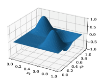
(a) Desired State

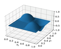
(b) Optimal State

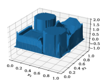
(c) Optimal Control

Figure 1: Example 1: The desired state ${y_{d}}$, the optimal state, and the optimal control (left to right).

We compare the different BB-type step-sizes presented in Section 2 with the baseline approach of using a fixed step-size in (1) and with a (non-)monotone linesearch approach. The results regarding computational time, function evaluations, and gradient-like evaluations are gathered in Table 2. For the linesearch methods, the most volatile of the novel BB-type step-size updates is used as baseline, i.e. BB1b.

	fixed	BB1a	BB2a	ABBa	BB1b	BB2b	ABBb	nonmon. LS (BB1b)	mon. LS (BB1b)
grad.-like eval.	$153662$	$618$	$1046$	$571$	$941$	$608$	$383$	$697$	$991$
fun. eval.	$0$	$0$	$0$	$0$	$0$	$0$	$0$	$887$	$1527$
$\text{time}[s]$	$1.56\cdot 10^{3}$	$1.01\cdot 10^{1}$	$1.36\cdot 10^{1}$	$1.55\cdot 10^{1}$	$8.39\cdot 10^{0}$	$7.92\cdot 10^{0}$	$5.65\cdot 10^{0}$	$2.21\cdot 10^{1}$	$3.30\cdot 10^{1}$

Table 2: Example 1: Numerical results for fixed step-size, different spectral gradient methods as introduced in Section 2, and a (non-)monotone linesearch method with respect to BB1b.

As can be seen from Table (2), for this example, all other approaches outperform the one with fixed step-size by a huge margin of about two orders of magnitude. The alternating BB-methods appear to be more efficient compared to the single BB-updates for both the old and novel step-sizes. Furthermore, the novel step-sizes do not always outperform the old ones, but in the superior alternating BB-method, they do by a significant margin. In other words, they are competitive to the old ones. All of these considerations are valid for both computational time and gradient-like evaluations. Function evaluations are only needed if a linesearch method is used. Compared to the baseline method BB1b, the nonmonotone linesearch method needs about $250$ fewer gradient-like evaluations, but this comes at the cost of $887$ additional function evaluations for the linesearch and this results in an increased overall computational time. Compared to a monotone linesearch, the nonmonotone approach performs significantly better. The convergence behavior is also visualized in Figure 2.

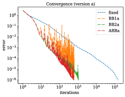
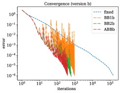
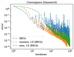
Figure 2: Example 1: Convergence of Algorithm 1. ”Error” refers to $\|{\mathcal{G}}_{\alpha_{k}}(u_{k})\|_{H}$ at the current iterate.

Figure 3 presents an example, where a BB-type step-size update without linesearch fails to converge. In this example, we start the algorithms with ${\alpha}_{0}=1$ instead of ${\alpha}_{0}=10$. This confirms the necessity of incorporating a linesearch strategy to ensure convergence.

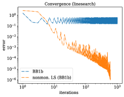
Figure 3: Example 1: Example of non-convergence without linesearch. ”Error” refers to $\|{\mathcal{G}}_{\alpha_{k}}(u_{k})\|_{H}$ at the current iterate.

Example 2 (Parabolic model problem)

In this example, we consider the model problem (P). Here, the spatial domain is discretized in the same manner as the one of the elliptic problem in Example 1. Moreover, for the temporal discretization, we use the Crank Nicolson/Adams Bashforth scheme MR2034880 . In this scheme, the implicit Crank Nicolson scheme is used except for the nonlinear terms which are treated using the explicit Adams Bashforth scheme and mass lumping. For the numerical tests we choose the parameters summarized in Table 3. Note that again for the fixed step-size approach ${\alpha}={\alpha}_{0}$ is used.

optimization problem

Algorithm 1

$\Omega$

$T$

$\kappa$

$\lambda$

$y_{d}$

${u_{a}}$

${u_{b}}$

$\varepsilon_{\mathrm{tol}}$

${\alpha}_{\inf}$

${\alpha}_{\sup}$

${\alpha}_{0}$

$\eta$

$\delta$

${m_{\mathrm{max}}}$

$(0,1)^{2}$

$1$

$10^{-2}$

$10^{-2}$

$\mathrm{see\;Figure\;\ref{fig:parabolic_desired}}$

$-100$

$100$

$10^{-6}$

$10^{-4}$

$10^{2}$

$10$

$4$

$0.8$

$4$

Table 3: Example 2: Parameter setting.

The desired state, the optimal state and the optimal control at time instances $t=0,0.25,0.5,0.75$ are depicted in Figures 6, 6, and 6, respectively. We can clearly see sparsity in space for the control. Note hat also sparsity in time can be observed in the sense that the control stays zero on an interval between time instances $t=0.25$ and $t=0.75$.

(a) $t=0$

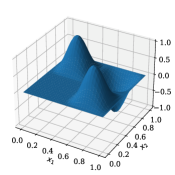
(b) $t=0.25$

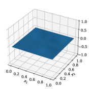
(c) $t=0.5$

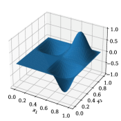
(d) $t=0.75$

Figure 4: Example 2: Snapshots of the desired state ${y_{d}}$ at time instances $0,0.25,0.5$ and $0.75$.

(a) $t=0$

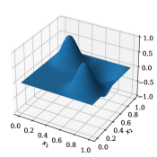
(b) $t=0.25$

(c) $t=0.5$

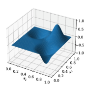
(d) $t=0.75$

Figure 5: Example 2: Snapshots of the optimal state at time instances $0,0.25,0.5$ and $0.75$.

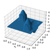
(a) $t=0$

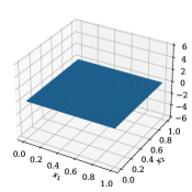
(b) $t=0.25$

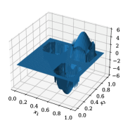
(c) $t=0.5$

(d) $t=0.75$

Figure 6: Example 2: Snapshots of the optimal control at time instances $0,0.25,0.5$ and $0.75$.

Similarly to Exmaple 1, we compare the different BB-type step-sizes presented in Section 2 with the baseline approach of using a fixed step-size and with a (non-)monotone linesearch approach, and the results regarding computational time, function evaluations and gradient-like evaluations are presented in Table 4. To reveal the efficiency of the linesearch strategy, we incorporated the least efficient BB-type step-size, namely BB1b with the linesearch strategy.

	fixed	BB1a	BB2a	ABBa	BB1b	BB2b	ABBb	nonmon. LS (BB1b)	mon. LS (BB1b)
grad.-like eval.	$515044$	$375$	$758$	$784$	$470$	$445$	$221$	$463$	$471$
fun. eval.	$0$	$0$	$0$	$0$	$0$	$0$	$0$	$639$	$713$
$\text{time}[s]$	$5.66\cdot 10^{4}$	$4.28\cdot 10^{1}$	$8.70\cdot 10^{1}$	$8.89\cdot 10^{1}$	$5.35\cdot 10^{1}$	$5.08\cdot 10^{1}$	$2.50\cdot 10^{1}$	$8.65\cdot 10^{1}$	$9.57\cdot 10^{1}$

Table 4: Example 2: Numerical results for fixed step-size, different spectral gradient methods as introduced in Section 2, and a (non-)monotone linesearch method with respect to BB1b.

All considerations and observations from Example 1 hold also true for this example. That is, the iterations (1) for the choice of the BB-type step-sizes significantly outperform those with fixed step-size, as is to be expected. The novel alternating BB-method outperforms the other approaches. The nonmonotone linesearch method outperforms the monotone version. It also outperforms the BB1b version with respect to gradient-like evaluations, but the cost of additional $639$ function evaluations again does not pay off with respect to overall computational time. The convergence behavior is also visualized in Figure 7.

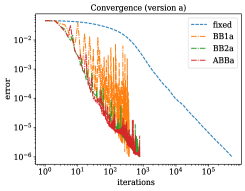
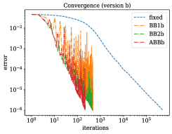
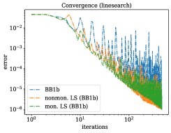
Figure 7: Example 2: convergence of Algorithm 1. ”Error” refers to $\|{\mathcal{G}}_{\alpha_{k}}(u_{k})\|_{H}$ at the current iterate.

To summarize, all the numerical results from the above examples show the capabilities of Algorithm 1 and the necessity for the use of a linesearch method. From the above example, we can conclude that the incorporation of nonmonotone linesearch and BB step-sizes leads to an efficient algorithm for a class of non-smooth PDE-constrained optimization problems. Moreover, the convergence behavior is far better than what our worst-case complexity results suggest. In particular, when combined with BB methods, this is typical behavior, see e.g., azmi_analysis_2020 ; MR967848 . Whether the strong quadratic growth condition helps to accelerate convergence in the elliptic example (E) towards the end is not entirely clear, although the orange curves in Figures 2 and 3 suggest it.

Conclusion

We have studied the nonmonotone FBS method for a class of infinite-dimensional composite problems in Hilbert spaces. Most prominently, we have established global convergence with complexity $(1/\sqrt{k})$ and also provide a complexity analysis. Under additional convexity assumption, convergence is now sublinear of order $(1/k)$ in function values. If additionally, a quadratic growth-type condition is satisfied, we have shown $R$-linear convergence, both in function values and iterates. Additional difficulties arising in the transition from weak to strong convergence in the infinite-dimensional setting have been discussed in detail. Finally, the nonmonotone FBS and the novel BB step-size rules exploiting the nonsmooth part were successfully tested for elliptic and parabolic PDE-constrained problems.

Appendix A Appendix

A.1 Proof of Theorem 3.2

Here, we restrict ourselves mainly to deriving (32). Justification of (33) follows by similar arguments. The proof is carried out by determining the minimum reduction of the objective function between iteration step $u_{k+1}$ and its maximal predecessor , i.e. $u_{\ell(k)}$, with respect to (12) as long as Algorithm 1 has not been terminated. Note that $u_{\ell(k)}$ can be calculated without further evaluations of the cost function by storing previous iterates. When using Algorithm 1, we have the following two cases:

• Assume that (9) in Step 4 of Algorithm (1) holds for $\alpha_{k}:={\alpha_{\mathrm{int},k}}$ and therefore $i_{k}=0$. Then we have a decrease

  $${\Psi}(u_{\ell(k)})-{\Psi}(u_{k+1})\geq\frac{\delta}{{\alpha_{\mathrm{int},k}}}\|{\mathcal{G}}_{\alpha_{k}}(u_{k})\|_{H}^{2}\geq\frac{\delta}{{\alpha}_{\sup}}\|{\mathcal{G}}_{\alpha_{k}}(u_{k})\|_{H}^{2}.$$

  In this case, only one additional function evaluation is necessary to obtain this decrease.

• Assume that (9) in Step 4 of Algorithm 1 fails to hold for ${\alpha_{\mathrm{int},k}}$ and therefore $i_{k}\geq 1$ backtracking steps are performed. Due to (iii) of Lemma 3 we have

  $$\alpha_{k}={\alpha_{\mathrm{int},k}}\eta^{i_{k}}<\frac{\eta{L_{{\mathcal{F}}^{\prime}}}}{2(1-\delta)},$$

  and, as a consequence, we can bound $i_{k}$ as follows

  $$i_{k}<\left|\log_{\eta}\left(\frac{\eta{L_{{\mathcal{F}}^{\prime}}}}{2{\alpha_{\mathrm{int},k}}(1-\delta)}\right)\right|.$$

  Hence, Step 4 requires at most $n_{1}\coloneqq\left\lfloor\left|\log_{\eta}\left(\frac{\eta{L_{{\mathcal{F}}^{\prime}}}}{2{\alpha}_{\inf}(1-\delta)}\right)\right|\right\rfloor$ function evaluations. At the time that the linesearch strategy terminates in this step, we have the decrease

  $${\Psi}(u_{\ell(k)})-{\Psi}(u_{k+1})\geq\frac{\delta}{\alpha_{k}}\|{\mathcal{G}}_{\alpha_{k}}(u_{k})\|_{H}^{2}>\frac{2(1-\delta)\delta}{\eta{L_{{\mathcal{F}}^{\prime}}}}\|{\mathcal{G}}_{\alpha_{k}}(u_{k})\|_{H}^{2}.$$

Gathering the two above cases, we can see that function value decrease per function evaluation is given, in the worst-case, by

$${\Psi}(u_{\ell(k)})-{\Psi}(u_{k+1})\geq\gamma_{\mathrm{decr}}\|{\mathcal{G}}_{\alpha_{k}}(u_{k})\|_{H}^{2}.$$

with $\gamma_{\mathrm{decr}}\coloneqq\min\left\{\frac{\delta}{{\alpha}_{\sup}},\frac{2(1-\delta)\delta}{n_{1}\eta{L_{{\mathcal{F}}^{\prime}}}}\right\}$. Further, using similar arguments as in the proof of Theorem 3.1, we obtain

$$\begin{split}&{\Psi}({u_{0}})-{\bar{\Psi}}\geq{\Psi}({u_{0}})-{\Psi}(u_{k})\geq{\Psi}{(u_{\nu(0)})}-{\Psi}(u_{\nu(\left\lceil\frac{k}{{m_{\mathrm{max}}}+1}\right\rceil)})\\ &=\sum^{\left\lceil\frac{k}{{m_{\mathrm{max}}}+1}\right\rceil}_{i=1}{\Psi}(u_{\nu(i-1)})-{\Psi}(u_{\nu(i)})\geq\sum^{\left\lceil\frac{k}{{m_{\mathrm{max}}}+1}\right\rceil}_{i=1}\gamma_{\mathrm{decr}}\|{\mathcal{G}}_{{\alpha}_{\nu(i)-1}}(u_{\nu(i)-1)})\|_{H}^{2}\\ &\geq\gamma_{\mathrm{decr}}\left\lceil\frac{k}{{m_{\mathrm{max}}}+1}\right\rceil\min_{1\leq i\leq\left\lceil\frac{k}{{m_{\mathrm{max}}}+1}\right\rceil}\|{\mathcal{G}}_{{\alpha}_{\nu(i)-1}}(u_{\nu(i)-1})\|^{2}_{H}\\ &\geq\left(\frac{\gamma_{\mathrm{decr}}k}{{m_{\mathrm{max}}}+1}\right)\min_{0\leq i\leq\left\lceil\frac{k}{{m_{\mathrm{max}}}+1}\right\rceil({m_{\mathrm{max}}}+1)-1}\|{\mathcal{G}}_{{\alpha}_{i}}(u_{i})\|^{2}_{H}\\ &\geq\left(\frac{\gamma_{\mathrm{decr}}k}{C^{2{m_{\mathrm{max}}}}_{G}({m_{\mathrm{max}}}+1)}\right)\min_{0\leq i\leq k}\|{\mathcal{G}}_{{\alpha}_{i}}(u_{i})\|^{2}_{H}.\end{split}$$ (82)

To find an $\varepsilon_{\mathrm{tol}}$-stationary point, we assume that up to the current iteration $k$ Algorithm 1 has not been terminated, i.e. $\|{\mathcal{G}}_{{\alpha}_{i}}(u_{i})\|_{H}>\epsilon$ for all $i=0,\dots,k$. In this case, using (82), we can write

$$\begin{split}&{\Psi}({u_{0}})-{\bar{\Psi}}>\left(\frac{\gamma_{\mathrm{decr}}k}{C^{2{m_{\mathrm{max}}}}_{G}({m_{\mathrm{max}}}+1)}\right)\varepsilon_{\mathrm{tol}}^{2},\end{split}$$

and, therefore, the total number of function evaluations of ${\Psi}$ in Algorithm 1 is bounded from above by

$$k_{\max}^{f}\leq\left\lfloor\frac{C^{2{m_{\mathrm{max}}}}_{G}({m_{\mathrm{max}}}+1)({\Psi}({u_{0}})-{\bar{\Psi}})}{\gamma_{\mathrm{decr}}\varepsilon_{\mathrm{tol}}^{2}}\right\rfloor=\left\lfloor\frac{\gamma_{\mathrm{comp}}^{f}({\Psi}({u_{0}})-{\bar{\Psi}})}{\varepsilon_{\mathrm{tol}}^{2}}\right\rfloor.$$

Thus, we are finished with the verification of (32). Similarly, using (24), it can be easily show that the total number of ${\mathcal{G}}_{\alpha_{k}}(u_{k})$ evaluations is bounded by

$$k_{\max}^{g}\leq\left\lfloor\frac{C^{2{m_{\mathrm{max}}}}_{G}\overline{{\alpha}}({m_{\mathrm{max}}}+1)({\Psi}({u_{0}})-{\bar{\Psi}})}{\delta\varepsilon_{\mathrm{tol}}^{2}}\right\rfloor=\left\lfloor\frac{\gamma_{\mathrm{comp}}^{g}({\Psi}({u_{0}})-{\bar{\Psi}})}{\varepsilon_{\mathrm{tol}}^{2}}\right\rfloor,$$

and, thus, the proof is complete.

A.2 Proof of Lemma 5

First, we show for every $k\geq 1$ that

$$\begin{split}{\Psi}(u_{k})\leq\min_{w\in{H}}\mathcal{Q}_{{\alpha}_{k-1}}(w,u_{k-1})+\frac{{L_{{\mathcal{F}}^{\prime}}}}{2{\alpha}_{\inf}{\alpha}_{k-1}}\|{\mathcal{G}}_{{\alpha}_{k-1}}(u_{k-1})\|_{H}^{2}.\end{split}$$ (83)

Due to A3:, the descent lemma, see (MR3310025, , Lemma 1.30), implies

$${\mathcal{F}}(u_{k})\leq{\mathcal{F}}(u_{k-1})+({\nabla{\mathcal{F}}}(u_{k}),u_{k}-u_{k-1})_{H}+\frac{{L_{{\mathcal{F}}^{\prime}}}}{2{\alpha}^{2}_{k-1}}\|{\mathcal{G}}_{{\alpha}_{k-1}}(u_{k-1})\|_{H}^{2}.$$

Using the definition of $\mathcal{Q}_{{\alpha}_{k-1}}$ and the fact that $u_{k}$ is the minimizer of $\mathcal{Q}_{{\alpha}_{k-1}}(\cdot,u_{k-1})$, we obtain

$$\begin{split}{\Psi}(u_{k})&\leq\min_{w\in{H}}\mathcal{Q}_{{\alpha}_{k-1}}(w,u_{k-1})+\left(\frac{{L_{{\mathcal{F}}^{\prime}}}}{2{\alpha}^{2}_{k-1}}-\frac{1}{2{\alpha}_{k-1}}\right)\|{\mathcal{G}}_{{\alpha}_{k-1}}(u_{k-1})\|_{H}^{2}\\ &\leq\min_{w\in{H}}\mathcal{Q}_{{\alpha}_{k-1}}(w,u_{k-1})+\frac{{L_{{\mathcal{F}}^{\prime}}}}{2{\alpha}^{2}_{k-1}}\|{\mathcal{G}}_{{\alpha}_{k-1}}(u_{k-1})\|_{H}^{2},\end{split}$$

and, thus, (83) follows from the fact that $\alpha_{k}\geq{\alpha}_{\inf}$ for all $k\in{\mathbb{N}}_{0}$.

Due to the convexity of ${\mathcal{F}}$, we can write

$$\min_{w\in{H}}\mathcal{Q}_{{\alpha}_{k-1}}(w,u_{k-1})\leq\min_{w\in{H}}\{{\Psi}(w)+\frac{{\alpha}_{k-1}}{2}\|w-u_{k-1}\|^{2}_{H}\}.$$ (84)

Further, due to the convexity of ${\Psi}$, we obtain for every $w=(1-\lambda)u_{k-1}+\lambda u^{*}$ with $\lambda\in[0,1]$ and $u^{*}\in{S_{*}}$ that

$$\begin{split}\min_{w\in{H}}&\{{\Psi}(w)+\frac{{\alpha}_{k-1}}{2}\|w-u_{k-1}\|^{2}_{H}\}\leq{\Psi}((1-\lambda)u_{k-1}+\lambda u^{*})+\frac{{\alpha}_{k-1}\lambda^{2}}{2}\|u_{k-1}-u^{*}\|^{2}_{H}\\ &\leq(1-\lambda){\Psi}(u_{k-1})+\lambda{\Psi}^{*}+\frac{{\alpha}_{k-1}\lambda^{2}}{2}\|u_{k-1}-u^{*}\|^{2}_{H}.\end{split}$$

Combining with (83) and (84), we obtain

$$\begin{split}{\Psi}(u_{k})&\leq(1-\lambda){\Psi}(u_{k-1})+\lambda{\Psi}^{*}+\frac{{\alpha}_{k-1}\lambda^{2}}{2}\|u_{k-1}-u^{*}\|^{2}_{H}+\frac{{L_{{\mathcal{F}}^{\prime}}}}{2{\alpha}_{\inf}{\alpha}_{k-1}}\|{\mathcal{G}}_{{\alpha}_{k-1}}(u_{k-1})\|_{H}^{2}\\ &\leq(1-\lambda){\Psi}(u_{\ell(k-1)})+\lambda{\Psi}^{*}+\frac{{\alpha}_{k-1}\lambda^{2}}{2}\|u_{k-1}-u^{*}\|^{2}_{H}+\frac{{L_{{\mathcal{F}}^{\prime}}}}{2{\alpha}_{\inf}{\alpha}_{k-1}}\|{\mathcal{G}}_{{\alpha}_{k-1}}(u_{k-1})\|_{H}^{2}.\end{split}$$ (85)

Now, inserting $\nu(k)$ in the place of $k$ in (85) and using (21), we obtain

$$\begin{split}{\Psi}(u_{\nu(k)})&\leq(1-\lambda){\Psi}(u_{\nu(k-1)})+\lambda{\Psi}^{*}+\frac{{\alpha}_{\nu(k)-1}\lambda^{2}}{2}\|u_{\nu(k)-1}-u^{*}\|^{2}_{H}\\ &+\frac{{L_{{\mathcal{F}}^{\prime}}}}{2{\alpha}_{\inf}{\alpha}_{\nu(k)-1}}\|{\mathcal{G}}_{{\alpha}_{\nu(k)-1}}(u_{\nu(k)-1})\|_{H}^{2}.\end{split}$$ (86)

Subtracting ${\Psi}^{*}$ from both sides of (86), setting $\tilde{C}:=\frac{{L_{{\mathcal{F}}^{\prime}}}}{2{\alpha}_{\inf}}$ and using (iii) of Lemma 3 we obtain

$$\begin{split}{\Psi}(u_{\nu(k)})-{\Psi}^{*}&\leq(1-\lambda)\left({\Psi}(u_{\nu(k-1)})-{\Psi}^{*}\right)+\frac{\overline{{\alpha}}\lambda^{2}}{2}\|u_{\nu(k)-1}-u^{*}\|^{2}_{H}\\ &+\frac{\tilde{C}}{{\alpha}_{\nu(k)-1}}\|{\mathcal{G}}_{{\alpha}_{\nu(k)-1}}(u_{\nu(k)-1})\|_{H}^{2}.\end{split}$$ (87)

Finally, (34) follows from the fact that $u^{*}\in{S_{*}}$ was arbitrary and ${S_{*}}$ is non-empty, closed, and convex.

Now we deal with the verification of (35). Let an arbitrary $u^{*}\in{S_{*}}$ be given, setting $k=1$ and $\lambda=1$ in (87), we obtain

$$\begin{split}{\Psi}(u_{\nu(1)})-{\Psi}^{*}\leq\frac{\overline{{\alpha}}}{2}\|u_{\nu(1)-1}-u^{*}\|^{2}_{H}+\frac{\tilde{C}}{{\alpha}_{\nu(1)-1}}\|{\mathcal{G}}_{{\alpha}_{\nu(1)-1}}(u_{\nu(1)-1})\|_{H}^{2}.\end{split}$$ (88)

Using, the fact that $0\leq\nu(1)-1\leq{m_{\mathrm{max}}}$ (see L1:), the firm non-expansiveness of the proximal operator, and the Lipschitz continuity of ${\nabla{\mathcal{F}}}$, we can write that

$$\begin{split}&\|u_{\nu(1)-1}-u^{*}\|_{H}\leq\left(1+\frac{{L_{{\mathcal{F}}^{\prime}}}}{{\alpha}_{\nu(1)-2}}\right)\|u_{\nu(1)-2}-u^{*}\|_{H}\\ &\leq\left(1+\frac{{L_{{\mathcal{F}}^{\prime}}}}{{\alpha}_{\inf}}\right)\|u_{\nu(1)-2}-u^{*}\|_{H}\leq\cdots\leq\left(1+\frac{{L_{{\mathcal{F}}^{\prime}}}}{{\alpha}_{\inf}}\right)^{{m_{\mathrm{max}}}}\|u_{0}-u^{*}\|_{H}.\end{split}$$ (89)

Further, using (iv) of Lemma 3 successively, we obtain that

$$\|{\mathcal{G}}_{{\alpha}_{\nu(1)-1}}(u_{\nu(1)-1})\|_{H}\leq C^{{m_{\mathrm{max}}}}_{G}\|{\mathcal{G}}_{{\alpha}_{0}}(u_{0})\|_{H}.$$ (90)

Combining (88), (89), and (90), we can write

$$\begin{split}{\Psi}(u_{\nu(1)})-{\Psi}^{*}&\leq\frac{\overline{{\alpha}}}{2}\left(1+\frac{{L_{{\mathcal{F}}^{\prime}}}}{{\alpha}_{\inf}}\right)^{2{m_{\mathrm{max}}}}\|u_{0}-u^{*}\|^{2}_{H}+\frac{\tilde{C}C^{2{m_{\mathrm{max}}}}_{G}}{{\alpha}_{\inf}}\|{\mathcal{G}}_{{\alpha}_{0}}(u_{0})\|_{H}^{2}\\ &\leq\frac{\overline{{\alpha}}}{2}\left(1+\frac{{L_{{\mathcal{F}}^{\prime}}}}{{\alpha}_{\inf}}\right)^{2{m_{\mathrm{max}}}}\|u_{0}-u^{*}\|^{2}_{H}+\frac{\overline{{\alpha}}^{2}\tilde{C}C^{2{m_{\mathrm{max}}}}_{G}}{{\alpha}_{\inf}}\|u_{1}-u_{0}\|_{H}^{2}.\end{split}$$ (91)

Further, the firm non-expansiveness of the proximal operator and the Lipschitz continuity of ${\nabla{\mathcal{F}}}$ again imply that

$$\begin{split}\|u_{1}-u_{0}\|_{H}&\leq\|u_{0}-u^{*}\|_{H}+\|u_{1}-u^{*}\|_{H}\\ &\leq 2\|u_{0}-u^{*}\|_{H}+\frac{{L_{{\mathcal{F}}^{\prime}}}}{{\alpha}_{0}}\|u_{0}-u^{*}\|_{H}\leq\big{(}2+\frac{{L_{{\mathcal{F}}^{\prime}}}}{{\alpha}_{\inf}}\big{)}\|u_{0}-u^{*}\|_{H}.\end{split}$$ (92)

Thus, combining (91) and (92) and setting

$$C_{0}\coloneqq\frac{\overline{{\alpha}}}{2}\left(1+\frac{{L_{{\mathcal{F}}^{\prime}}}}{{\alpha}_{\inf}}\right)^{2{m_{\mathrm{max}}}}+\frac{\overline{{\alpha}}^{2}\tilde{C}C^{2{m_{\mathrm{max}}}}_{G}}{{\alpha}_{\inf}}\big{(}2+\frac{{L_{{\mathcal{F}}^{\prime}}}}{{\alpha}_{\inf}}\big{)}^{2},$$

we arrive at

$${\Psi}(u_{\nu(1)})-{\Psi}^{*}\leq C_{0}\|u_{0}-u^{*}\|^{2}_{{H}}.$$

Hence, (35) follows from the fact that $u^{*}\in{S_{*}}$ is arbitrary.

References

• (1) Ahookhosh, M., Themelis, A., Patrinos, P.: A Bregman forward-backward linesearch algorithm for nonconvex composite optimization: superlinear convergence to nonisolated local minima. SIAM J. Optim. 31(1), 653–685 (2021). DOI 10.1137/19M1264783. URL https://doi.org/10.1137/19M1264783
• (2) Alber, Y.I., Iusem, A.N., Solodov, M.V.: On the projected subgradient method for nonsmooth convex optimization in a Hilbert space. Math. Program. 81(1 (A)), 23–35 (1998). DOI 10.1007/BF01584842
• (3) Allgower, E.L., Böhmer, K.: Application of the mesh independence principle to mesh refinement strategies. SIAM J. Numer. Anal. 24(6), 1335–1351 (1987). DOI 10.1137/0724086. URL http://dx.doi.org/10.1137/0724086
• (4) Allgower, E.L., Böhmer, K., Potra, F.A., Rheinboldt, W.C.: A mesh-independence principle for operator equations and their discretizations. SIAM J. Numer. Anal. 23(1), 160–169 (1986). DOI 10.1137/0723011. URL http://dx.doi.org/10.1137/0723011
• (5) Alnæs, M., Blechta, J., Hake, J., Johansson, A., Kehlet, B., Logg, A., Richardson, C., Ring, J., Rognes, M.E., Wells, G.N.: The fenics project version 1.5. Archive of Numerical Software 3(100) (2015)
• (6) Artacho, F.A., Geoffroy, M.H.: Characterization of metric regularity of subdifferentials. Journal of Convex Analysis 15(2), 365 (2008)
• (7) Artacho, F.J.A., Geoffroy, M.H.: Metric subregularity of the convex subdifferential in Banach spaces. J. Nonlinear Convex Anal. 15(1), 35–47 (2014). URL www.yokohamapublishers.jp/online2/opjnca/vol15/p35.html
• (8) Attouch, H., Bolte, J.: On the convergence of the proximal algorithm for nonsmooth functions involving analytic features. Math. Program. 116(1-2 (B)), 5–16 (2009). DOI 10.1007/s10107-007-0133-5
• (9) Attouch, H., Bolte, J., Svaiter, B.F.: Convergence of descent methods for semi-algebraic and tame problems: proximal algorithms, forward-backward splitting, and regularized Gauss-Seidel methods. Math. Program. 137(1-2 (A)), 91–129 (2013). DOI 10.1007/s10107-011-0484-9
• (10) Azmi, B., Kunisch, K.: Analysis of the Barzilai-Borwein Step-Sizes for Problems in Hilbert Spaces. Journal of Optimization Theory and Applications 185(3), 819–844 (2020). DOI 10.1007/s10957-020-01677-y. URL https://doi.org/10.1007/s10957-020-01677-y
• (11) Azmi, B., Kunisch, K.: On the convergence and mesh-independent property of the Barzilai–Borwein method for PDE-constrained optimization. IMA Journal of Numerical Analysis (2021). DOI 10.1093/imanum/drab056. URL https://doi.org/10.1093/imanum/drab056. Drab056
• (12) Azmi, B., Kunisch, K., Rodrigues, S.S.: Saturated feedback stabilizability to trajectories for the schlögl parabolic equation. IEEE Transactions on Automatic Control pp. 1–14 (2023). DOI 10.1109/TAC.2023.3247511
• (13) Azé, D., Corvellec, J.N.: Nonlinear local error bounds via a change of metric. Journal of Fixed Point Theory and Applications 16(1-2), 351–372 (2014). DOI 10.1007/s11784-015-0220-9. URL http://link.springer.com/10.1007/s11784-015-0220-9
• (14) Barzilai, J., Borwein, J.M.: Two-point step size gradient methods. IMA J. Numer. Anal. 8(1), 141–148 (1988). DOI 10.1093/imanum/8.1.141. URL https://doi.org/10.1093/imanum/8.1.141
• (15) Bauschke, H.H., Combettes, P.L.: Convex analysis and monotone operator theory in Hilbert spaces, second edn. CMS Books in Mathematics/Ouvrages de Mathématiques de la SMC. Springer, Cham (2017). DOI 10.1007/978-3-319-48311-5. URL https://doi.org/10.1007/978-3-319-48311-5. With a foreword by Hédy Attouch
• (16) Beck, A.: First-order methods in optimization, MOS/SIAM Ser. Optim., vol. 25. Philadelphia, PA: Society for Industrial and Applied Mathematics (SIAM); Philadelphia, PA: Mathematical Optimization Society (MOS) (2017). DOI 10.1137/1.9781611974997
• (17) Beck, A., Teboulle, M.: A fast iterative shrinkage-thresholding algorithm for linear inverse problems. SIAM J. Imaging Sci. 2(1), 183–202 (2009). DOI 10.1137/080716542. URL semanticscholar.org/paper/bcf48b5e76c7e22335c6820f0de0abe8c5f708b5
• (18) Bello-Cruz, Y., Li, G., Nghia, T.T.A.: On the linear convergence of forward-backward splitting method: Part I—Convergence analysis. J. Optim. Theory Appl. 188(2), 378–401 (2021). DOI 10.1007/s10957-020-01787-7. URL https://doi.org/10.1007/s10957-020-01787-7
• (19) Bello-Cruz, Y., Li, G., Nghia, T.T.A.: Quadratic growth conditions and uniqueness of optimal solution to lasso. J. Optim. Theory Appl. 194(1), 167–190 (2022). DOI 10.1007/s10957-022-02013-2. URL https://doi.org/10.1007/s10957-022-02013-2
• (20) Boţ, R.I., Csetnek, E.R., László, S.C.: An inertial forward-backward algorithm for the minimization of the sum of two nonconvex functions. EURO J. Comput. Optim. 4(1), 3–25 (2016). DOI 10.1007/s13675-015-0045-8. URL https://doi.org/10.1007/s13675-015-0045-8
• (21) Bolte, J., Nguyen, T.P., Peypouquet, J., Suter, B.W.: From error bounds to the complexity of first-order descent methods for convex functions. Math. Program. 165(2, Ser. A), 471–507 (2017). DOI 10.1007/s10107-016-1091-6. URL https://doi.org/10.1007/s10107-016-1091-6
• (22) Bonettini, S., Loris, I., Porta, F., Prato, M.: Variable metric inexact line-search-based methods for nonsmooth optimization. SIAM J. Optim. 26(2), 891–921 (2016). DOI 10.1137/15M1019325. URL https://doi.org/10.1137/15M1019325
• (23) Cartis, C., Sampaio, P.R., Toint, P.L.: Worst-case evaluation complexity of non-monotone gradient-related algorithms for unconstrained optimization. Optimization 64(5), 1349–1361 (2015). DOI 10.1080/02331934.2013.869809. URL citeseerx.ist.psu.edu/viewdoc/summary?doi=10.1.1.726.1663
• (24) Casas, E.: Second order analysis for bang-bang control problems of pdes. SIAM Journal on Control and Optimization 50(4), 2355–2372 (2012). DOI 10.1137/120862892
• (25) Casas, E.: A review on sparse solutions in optimal control of partial differential equations. SeMA Journal 74(3), 319–344 (2017)
• (26) Casas, E., Mateos, M., Rösch, A.: Analysis of control problems of nonmontone semilinear elliptic equations. ESAIM Control Optim. Calc. Var. 26, Paper No. 80, 21 (2020). DOI 10.1051/cocv/2020032. URL https://doi.org/10.1051/cocv/2020032
• (27) Combettes, P.L.: Quasi-fejérian analysis of some optimization algorithms. In: D. Butnariu, Y. Censor, S. Reich (eds.) Inherently Parallel Algorithms in Feasibility and Optimization and their Applications, Studies in Computational Mathematics, vol. 8, pp. 115–152. Elsevier (2001). DOI https://doi.org/10.1016/S1570-579X(01)80010-0. URL https://www.sciencedirect.com/science/article/pii/S1570579X01800100
• (28) Combettes, P.L., Pesquet, J.C.: Proximal splitting methods in signal processing. In: Fixed-point algorithms for inverse problems in science and engineering, Springer Optim. Appl., vol. 49, pp. 185–212. Springer, New York (2011). DOI 10.1007/978-1-4419-9569-8“˙10. URL https://doi.org/10.1007/978-1-4419-9569-8_10
• (29) Dontchev, A.L., Zolezzi, T.: Well-posed optimization problems, Lect. Notes Math., vol. 1543. Berlin: Springer-Verlag (1993)
• (30) Drusvyatskiy, D., Lewis, A.S.: Error bounds, quadratic growth, and linear convergence of proximal methods. Math. Oper. Res. 43(3), 919–948 (2018). DOI 10.1287/moor.2017.0889. URL https://doi.org/10.1287/moor.2017.0889
• (31) Drusvyatskiy, D., Mordukhovich, B.S., Nghia, T.T.A.: Second-order growth, tilt stability, and metric regularity of the subdifferential. J. Convex Anal. 21(4), 1165–1192 (2014). URL www.heldermann.de/JCA/JCA21/JCA214/jca21061.htm
• (32) Frankel, P., Garrigos, G., Peypouquet, J.: Splitting methods with variable metric for Kurdyka-łojasiewicz functions and general convergence rates. J. Optim. Theory Appl. 165(3), 874–900 (2015). DOI 10.1007/s10957-014-0642-3. URL https://doi.org/10.1007/s10957-014-0642-3
• (33) Garrigos, G., Rosasco, L., Villa, S.: Thresholding gradient methods in Hilbert spaces: support identification and linear convergence. ESAIM: Control, Optimisation and Calculus of Variations 26, 28 (2020). DOI 10.1051/cocv/2019011. URL https://www.esaim-cocv.org/10.1051/cocv/2019011
• (34) Garrigos, G., Rosasco, L., Villa, S.: Convergence of the forward-backward algorithm: beyond the worst-case with the help of geometry. Mathematical Programming (2022). DOI 10.1007/s10107-022-01809-4. URL https://doi.org/10.1007/s10107-022-01809-4
• (35) Grippo, L., Lampariello, F., Lucidi, S.: A nonmonotone line search technique for Newton’s method. SIAM J. Numer. Anal. 23(4), 707–716 (1986). DOI 10.1137/0723046. URL https://doi.org/10.1137/0723046
• (36) Hager, W.W., Phan, D.T., Zhang, H.: Gradient-based methods for sparse recovery. SIAM J. Imaging Sci. 4(1), 146–165 (2011). DOI 10.1137/090775063. URL https://doi.org/10.1137/090775063
• (37) He, Y.: Two-level method based on finite element and Crank-Nicolson extrapolation for the time-dependent Navier-Stokes equations. SIAM J. Numer. Anal. 41(4), 1263–1285 (2003). DOI 10.1137/S0036142901385659. URL https://doi.org/10.1137/S0036142901385659
• (38) Heinkenschloss, M.: Mesh independence for nonlinear least squares problems with norm constraints. SIAM J. Optim. 3(1), 81–117 (1993). DOI 10.1137/0803005. URL http://dx.doi.org/10.1137/0803005
• (39) Hintermüller, M., Ulbrich, M.: A mesh-independence result for semismooth Newton methods. Math. Program. 101(1, Ser. B), 151–184 (2004). URL https://doi.org/10.1007/s10107-004-0540-9
• (40) Hinze, M., Kunisch, K.: Second order methods for optimal control of time-dependent fluid flow. SIAM J. Control Optim. 40(3), 925–946 (2001). DOI 10.1137/S0363012999361810. URL https://doi.org/10.1137/S0363012999361810
• (41) Hinze, M., Pinnau, R., Ulbrich, M., Ulbrich, S.: Optimization with PDE Constraints. Mathematical Modelling: Theory and Applications. Springer Netherlands (2008). URL https://books.google.de/books?id=PFbqxa2uDS8C
• (42) Hüther, B.: Global convergence of algorithms with nonmonotone line search strategy in unconstrained optimization. Results Math. 41(3-4), 320–333 (2002). DOI 10.1007/BF03322774. URL https://doi.org/10.1007/BF03322774
• (43) Kanzow, C., Mehlitz, P.: Convergence properties of monotone and nonmonotone proximal gradient methods revisited. J. Optim. Theory Appl. 195(2), 624–646 (2022). DOI 10.1007/s10957-022-02101-3. URL https://doi.org/10.1007/s10957-022-02101-3
• (44) Kelley, C.T., Sachs, E.W.: Quasi-Newton methods and unconstrained optimal control problems. SIAM J. Control Optim. 25(6), 1503–1516 (1987). DOI 10.1137/0325083. URL http://dx.doi.org/10.1137/0325083
• (45) Kelley, C.T., Sachs, E.W.: Approximate quasi-Newton methods. Math. Programming 48(1, (Ser. B)), 41–70 (1990). URL https://doi.org/10.1007/BF01582251
• (46) Kunisch, K., Rodrigues, S.S.: Global stabilizability to trajectories for the schlögl equation in a sobolev norm (2022). DOI 10.48550/ARXIV.2212.01888. URL https://arxiv.org/abs/2212.01888
• (47) Li, G., Pong, T.K.: Global convergence of splitting methods for nonconvex composite optimization. SIAM J. Optim. 25(4), 2434–2460 (2015). DOI 10.1137/140998135. URL https://doi.org/10.1137/140998135
• (48) Mordukhovich, B.S.: Variational analysis and generalized differentiation. I: Basic theory. II: Applications, Grundlehren Math. Wiss., vol. 330/331. Berlin: Springer (2005). DOI 10.1007/3-540-31247-1
• (49) Necoara, I., Nesterov, Y., Glineur, F.: Linear convergence of first order methods for non-strongly convex optimization. Mathematical Programming 175(1-2), 69–107 (2019). DOI 10.1007/s10107-018-1232-1. URL http://link.springer.com/10.1007/s10107-018-1232-1
• (50) Nesterov, Y.: Gradient methods for minimizing composite functions. Math. Program. 140(1 (B)), 125–161 (2013). DOI 10.1007/s10107-012-0629-5
• (51) O’Donoghue, B., Stathopoulos, G., Boyd, S.: A splitting method for optimal control. IEEE Transactions on Control Systems Technology 21(6), 2432–2442 (2013). DOI 10.1109/TCST.2012.2231960
• (52) Parikh, N., Boyd, S., et al.: Proximal algorithms. Foundations and trends® in Optimization 1(3), 127–239 (2014)
• (53) Peypouquet, J.: Convex optimization in normed spaces. SpringerBriefs in Optimization. Springer, Cham (2015). DOI 10.1007/978-3-319-13710-0. URL https://doi.org/10.1007/978-3-319-13710-0. Theory, methods and examples, With a foreword by Hedy Attouch
• (54) Salzo, S.: The variable metric forward-backward splitting algorithm under mild differentiability assumptions. SIAM J. Optim. 27(4), 2153–2181 (2017). DOI 10.1137/16M1073741. URL https://doi.org/10.1137/16M1073741
• (55) Schirotzek, W.: Nonsmooth analysis. Universitext. Berlin: Springer (2007). DOI 10.1007/978-3-540-71333-3
• (56) Themelis, A., Stella, L., Patrinos, P.: Forward-backward envelope for the sum of two nonconvex functions: further properties and nonmonotone linesearch algorithms. SIAM J. Optim. 28(3), 2274–2303 (2018). DOI 10.1137/16M1080240. URL https://doi.org/10.1137/16M1080240
• (57) Virtanen, P., Gommers, R., Oliphant, T.E., Haberland, M., Reddy, T., Cournapeau, D., Burovski, E., Peterson, P., Weckesser, W., Bright, J., et al.: Scipy 1.0: fundamental algorithms for scientific computing in python. Nature methods 17(3), 261–272 (2020)
• (58) Volkwein, S.: Mesh-independence for an augmented Lagrangian-SQP method in Hilbert spaces. SIAM J. Control Optim. 38(3), 767–785 (2000). DOI 10.1137/S0363012998334468. URL http://dx.doi.org/10.1137/S0363012998334468
• (59) Wright, S.J., Nowak, R.D., Figueiredo, M.A.T.: Sparse reconstruction by separable approximation. IEEE Trans. Signal Process. 57(7), 2479–2493 (2009). DOI 10.1109/TSP.2009.2016892. URL https://doi.org/10.1109/TSP.2009.2016892