Observational Data on several close single Dwarfs of late spectral Classes where obtaned by the RATAN-600 Radio Telescope in Spring 2018.

Abstract

In April-May 2018, the RATAN-600 radio telescope carried out monitoring observations of 16 solar-like nearby star systems in four frequency bands. Registration was carried out with an increased sampling frequency of $\sim 18$ Hz. An algorithm for data processing in the mode of source passing through the radiation pattern by the method of dispersion analysis with noise filtering is described. The processing took into account the correction of the transit time for the secular shift of the right ascension of the sources due to their relative proximity. There have been several unidentified cases of anomalous excess of the standard deviation of noise from stationary values. For the most sensitive receivers in the 2.68 and 6.38 cm bands, this anomaly detection threshold with a 99% probability was $\sim 100$ mJy.

I Introduction.

The discovery of planetary systems near the stars closest to the Earth warmed up the area of research interest in assessing the non-stationarity of the level of radiation impact on them from the mother starYang et al. [2017], as a possibly significant factor for the possibility of the appearance of extraterrestrial life forms. Observations of stars in centimeter radio band with high time resolution is quite few, although, along with X-rays, they make it possible to record the flare activity of their atmospheres, similarly to the study of solar flares.

RATAN-600 has a large aperture and highly sensitive centimeter range radiometers. Although it operates primarily as a transit-mode source survey instrument, it can detect mJy-level fluctuations in the path of the source through the antenna pattern. The width of the antenna radiation pattern in terms of transit time, depending on the observed height and wavelength, ranges from several seconds to half a minute. The duration of observation of stars in this cycle are presented in the table LABEL:Result.

II Researched objects and purpose.

Star systems of 16 dwarfs with discovered planets in the supposed zone of existence of life forms were selected for observations. The list of stars is given in table LABEL:Result of the appendix. It is supposed to establish upper limits for the flux density for detecting the radio emission of the listed stellar systems in the series of observations on the Southern Sector of RATAN-600.

III Observation conditions and equipment.

The observations were carried out in the spring months in the interval from 04/06/2018 to 05/07/2018 mainly at night. Observation mode - Southern sector with a flat reflector, movable feed – secondary mirror N^o2 with daily rolling on rails to combine with other observational programs. A standard set of “Eridan-2”Berlin et al. [2012] radiometers was used, the central wavelengths of which are 1.38, 2.68, 6.38, and additionally a 13.33cm radiometer. The recording was made by the acquisition system Tsybulev [2011] in an accelerated mode with a sample rate of about 18 Hz (period $\sim 54.8ms$) for each frequency channel. Each radiometer used one horn each, the location and horizontal offsets from the focus of which are presented in Table 1. A carriage with radiometers during the passage of sources through the “knife” pattern the antenna is fixed, that is, the possibility signal accumulation in a single observation is determined only by its width in each of the four frequency channels. Since the mode of operation of the receiving paths is modulation, a separate record was formed for each of the two half-cycles of the modulation. The resulting single observation file for each radiometer was the vector sum of these records. Separate viewing of each of the summarized records allows you to identify and identify a class of very narrow impulse noise in case of detection anomalies in statistical properties receiving signal.

Table 1: Position of radiometer horns on secondary mirror carriage.

Radiometer, wavelendth$\lambda$ cm.	Horn position	Horisontal offset cm.
1.38	eastern	-1.35
2.68	west	5.05
6.38	west	12.9
13.33	west	34.3

IV Format of source records and software toolkit.

The purpose of processing the records of this observation cycle was to identify changes in the statistical properties of noise signal during the passage of the source through the antenna pattern. Changes were assessed in relation to the same intervals before and after prescribing the source. Due to the fact that a possible signal is hidden behind the usual noise recording, it is important to accurately calculate the start and end times of the analysis. Measurements of the variation of the coordinates of the position of the maximum by strong reference sources showed that the contribution of the receiver horn setting error, the contribution of noise, atmospheric refraction, and time synchronization does not exceed 0.1 s, which is commensurate with the sampling period of the recording. Some biggest error introduces a shift in the catalog value of the right ascension $Pm\_RA$ of the studied stars due to proper motion, which we have taken into account. We used the precomputed TIMEESH or TIMEWSH, respectively for the passage of the “east” or “west” working horns that are included in the header F-file data acquisition system. Also in analysis intervals were calculated using the values of the following parameters: LAMBDA – central wavelength, AZIMUTH – observation azimuth, OBSRA – right ascension of the source (excluding proper motion), OBSDEC - declination, XBFWHM - predicted transit time interval width source through the antenna pattern at half power.

The resulting time shift of the moment passing through the maximum of the Directivity diagram for each recording channel is determined by the following formula:

$$ts_{\lambda}=\frac{TS-0.018~{}Pm\_RA}{15~{}cos(OBSDEC~{}\pi/180)}$$ (1)

In expression (1) the 18th year is entered observations relative to the coordinates of RA2000 with the conversion of the dimension of the values of arcseconds into seconds of time. The TS value is equal to the TIMEESH or TIMEWSH values, up to the sign: $+$ or $-$, depending on the AZIMUTH and the location of the horn in the orientation of the three-mirror observing system, see table 1. As a result, we obtain the following formulas for calculating the average moments of time of the analyzed sections of the record:

$$t0_{\lambda}=3600~{}OBSRA-3~{}XBFWHM_{\lambda}+ts_{\lambda}$$ (2)

$$t1_{\lambda}=3600~{}OBSRA+XBFWHM_{\lambda}+ts_{\lambda}$$ (3)

$$t2_{\lambda}=3600~{}OBSRA+3~{}XBFWHM_{\lambda}+ts_{\lambda}$$ (4)

t is obvious that the initial and final moments of the analysis are obtained by subtracting and adding to the calculation centers the value of the half-width of the antenna pattern: $XBFWHM_{\lambda}$. The given data, together with the original multi-frequency files, are the input for the FADPS-basedVerkhodanov et al. [1993] software package.

V Computational procedures.

We processed the observations according to the well-known method of analysis of variance Cramér [1999]. Note that the Fisher test used to compare the variance is sensitive to the “normality” of the original distribution of noise samples in the input signal recording. Therefore, especially for the 13cm receiver, a rejection procedure is mandatory - censoring of recordings affected by earthly noise. Anomalous noises can greatly weight the right “tail” of the density of the sample probability distribution, shifting its center. So Fig.1 shows a typical histogram of the distribution density of the root of the sample noise variance y in the record J1718-3459(GJ667C) at a wavelength of 13.33 cm.

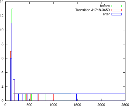
Figure 1: PDD histogram for a sample of $\sigma$ (mK) record of GJ667C at 13.33 cm from 26 observations.

We used well-known robust procedures to calculate the center of mass $X_{center}$ of the sample probability distribution of the resulting $\sigma$, based on the calculation of several rank statistics and the selection of the median value from them (Bulashev [2003]). A recording was considered uncorrupted by interference if:

$$X_{center}-G\cdot\tilde{\sigma}\leq\sigma\leq X_{center}+G\cdot\tilde{\sigma}$$ (5)

Where the censoring coefficient G is calculated by the empirical formula:

$$G=1.55+0.8\log(N/10)\cdot\sqrt{\epsilon-1}$$ (6)

Here the sample size is $N$, $\tilde{\sigma}$ is the estimate of the standard deviation from $X_{center}$ , and $\epsilon$ kurtosis estimate. The key stages of record processing are shown in the diagram in Figure 2.

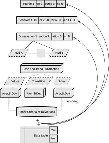
Figure 2: Data processing pipeline.

Choosing the analyzed source of observations and perform the following steps in a loop for all sources. Let’s transform a multi-frequency file into a set of single-part, single-channel. Let us choose for analysis a single-frequency record of the corresponding receiver: 1.38 cm, 2.68 cm, 6.38 cm and 13.33 cm. We choose one observation and perform pairwise vector addition of the channel recording files from two opposite modulation phases. We repeat this step and the next for all observations. We cut out a part of the record of the full interval for analysis, subtract the base level and the linear trend from it. Thus, we discard sections of the record with the inclusion of the calibration noise generator and their normalization by sample size, which reduces the influence of the slow component of the temperature trend and atmospheric noise on the resulting statistics. We cut out three sections of records from the resulting files according to the expressions 2,3,4. The length and, accordingly, the number of samples for each section of the record corresponds to the time of passage of a point source through twice the width (at the level of 0.5 power) of the horizontal dimension of the telescope beam pattern. Further for each segment of the record we calculate estimates of the mean – $\tilde{x}$ and standard deviation – $\sigma$. We enter the results in the table, including the value of the sample size. We compare the $\sigma$ of the analyzed areas and conclude that the null hypothesis is true: the equality of $\sigma$ according to the Fisher criterion. We write in the table the results of comparing $\sigma_{t1}$ with $\sigma_{t0}$ and $\sigma_{t2}$. We single out anomaly if the null hypothesis is rejected with a probability of 0.99. We repeat the calculations from the very beginning for the next observation. We calculate $\tilde{x}$, $\sigma$ from the observation cycle for a given radiometer wave. We censor the resulting sample for bounces of $\sigma$ values from the general population. The analysis is carried out for ”out-of-diagram” intervals: t0 and t2, in order to eliminate obvious interferences that distorts the statistics. It should be noted again that only those records affected by interference are discarded, in which the dispersion is anomalous precisely for the control sections before or after the source passes through the radiation pattern. That is, these are clearly not cases of the possible detection of radiation from the source under study. We compute an upper limit on the $\sigma$ estimate with a probability of 0.99, assuming that the initial $\chi^{2}$ is the population distribution for the variance estimate. We calculate the upper limit for estimating the average in the transit interval with a probability of 0.99, assuming that the initial $\tau$ is a Student’s distribution with censoring taken into account. We repeat the calculations starting with the choice of the receiver, and again a full cycle for each source. Note that the computations of each of the loops are unconditional and therefore can be easily parallelized. In order to convert the obtained results of the analysis from the units of noise temperature into the spectral flux density, we processed the calibration sources. We tried to include observation settings for known strong radio sources with the longest series of observations close in height. These are: 3C48, J0237-23, 3C138, 3C147, 3C161, J1154-35, 3C286, 4C+12.50, 3C295, J1850-0101, NGC7027. For the calculation, we used published data collected in the CATS Verkhodanov et al. [2009] database. Calibration method did not differ from the standard one, based on the calculation of the effective area of the antenna with the construction of its dependence on the height of the installation and is described, for example, in the work of Panov et al. Panov et al. [2019].

DISCUSSION OF OBSERVATIONS

Tau Cet e

The star Judge et al. [2004] with $Pm\_RA=-1721.94~{}mass/yr$, so the RA shift in the carriage position must be taken into account. The height is about $30^{\circ}$ above the horizon, due to which the capture of ground-based sources of interference is likely: thunderclouds, aircraft. 2 days of observations. Noteworthy day 04/07/2018: An impulse enters the initial region of passage by the diagram at 2.68cm, its Gaussian approximation is given in the table 2.

Table 2: Pulse parameters in the record Tau Cet e 04/07/2018. Wave 2.68cm. Top line: value, bottom line - approximation error.

Object: 0144-1556	Lambda: 2.68[cm]		Date: 07/04/18
[ h:m:s.s ]	[ mK ]	[ s ]	[ K*s ]
01:44:53.61 0.0125	124.87 28.5	0.091354 0.0125	0.012143

Its duration is slightly more than two counts and at the peak flux density is not less than 434 mJy, which is more than $5\sigma$ outside the passage (80.5 mJy). It is noteworthy that there is also an outlier at 6.28cm with a spacing along the “stellar” time less than a second. See table 3.

Table 3: Pulse parameters in the record Tau Cet e 04/07/2018. Wave 6.28cm. Top line: value, bottom line - approximation error.

Object: 0144-1556	Lambda: 6.28 [cm]		Date: 07/04/18
[ h:m:s.s ]	[ mK ]	[ s ]	[ K*s ]
01:44:51.81 0.0182	58.771 9.84	0.20123 0.0182	0.012589

Here, the pulse flux density is 229 mJy, which is more than $3\sigma$ (74 mJy). Duration in 4 counts. It is rather strange (for a thunderstorm) that there was no interference at 13.3cm that day, so on 04/07/2018 $\sigma$ noise in the passage: 141.451 mK, and on 04/09/2018 743.288 mK. That is, from ground interference, an overflight of the aircraft is most likely. However, in this case, the nature of the broadband properties of the pulse remains unclear. There were no responses comparable with the diagram in terms of width either on April 7th or on April 9th.

GJ3293d

An M-class dwarf Soubiran et al. [2018] with $Pm\_RA=-87~{}mas/yr$ was observed three days April 7-9. The height above the horizon is $21^{\circ}$, so the probability of trapping ground interferences by the antenna pattern is also very high. Only the 3rd day is remarkable: at 6.28cm, in the zone of passage through the diagram directivity due to a single-sawtooth pulse an increase in $\sigma$ noise temperature was observed. The parameters of approximation of this pulse by two Gaussians are presented in the table 4.

Table 4: Double pulse parameters in the entry GJ3293d 04/09/2018. Wave 6.28cm. Top line: value, bottom line - approximation error.

Object: 0428-2510	Lambda: 6.28[cm]		Date: 09/04/18
[ h:m:s.s ]	[ mK ]	[ s ]	[ K*s ]
04:29:17.43 0.0114 04:29:18.29 0.009	97.36 1.42 122.91 4.20	1.299 0.0114 0.4389 0.009	0.1347 0.0574

If the radio emission pulse is of a non-interference nature, then the density value flux per pulse is slightly above 2$\sigma$ of background noise.

GJ180c

A star systemFeng et al. [2020] with M3V class dwarf, its $Pm\_RA=408~{}mas/yr$ Gaia Collaboration et al. [2018]. Three passages were observed, and no anomalous increases in $\sigma$ were recorded.

GJ273b

Leuthen’s Star Vyssotsky [1943], a red dwarf of spectral class M3.5V, its $Pm\_RA=572~{}mas/yr$ Gaia Collaboration et al. [2018]. We observed 26 passages without any significant increase in $\sigma$ noise.

K2-18b

M2.5-class red dwarf with $Pm\_RA=-87.377~{}mas/yr$ Gaia Collaboration et al. [2018]. The sources 2MASS J11301676+0733404 Mag 15.5(g) and the quasar QSO B1127+078 (down $\delta$ by $2^{\prime}$), 113017.3818+073213.0294 (J2000) Mag 14.6 may fall into the RATAN-600 diagram lower in $\delta$ (K). At a wave of 6.38cm, the vertical half-width of the diagram in this case is about $2^{\circ}$. What could affect the determination of the upper limit of detection of the density of the radio emission flux from the star itself. Processing of 26 records showed that without compression (dt=0.054c), almost all days of $\sigma$ before, during and after the passage of the radiation pattern are identical according to the Fisher criterion with a probability of more than 95The exception is the recording of April 20, 2018, where, in the last interval of the analysis, an interference spike was detected at a wavelength of 6.38 cm with a duration of 0.375 s, much shorter than the half-width of the diagram, and an intensity of $4\sigma$ of background noise. On a wave of 1.38cm, anomalous days: 04/07/2018 and 05/03/2018, the sigma in the passage increased 1.3 and 1.8 times, respectively.

K2-9b

M2.5V class dwarf, source in 2MASS catalog J11450348+0000190 Kirkpatrick [2003], $Pm\_RA=-170.752~{}mas/yr$. 19 passages were observed. During the passage on 04/20/2018 in the 13.3 cm band, an interference in the form of a double pulse was registered, the approximation parameters of which are given in the table 5.

Table 5: Double pulse parameters in record K2-9b 04/20/2018. Wave 13cm. Top line: value, bottom line - approximation error.

Object: 1145-0000	Lambda: 13.33[cm]		Date: 20/04/18
[ h:m:s.s ]	[ mK ]	[ s ]	[ K*s ]
11:46:04.08 0.0021 11:46:04.94 0.0005	3522 43.4 14183 23.3	0.283 0.002 0.52759 0.0005	1.0616 7.965

Since the shape of the noise fits well into the highly compressed in time section of the radiation pattern with offset from the focus, then most likely this is the response to the passage of an aircraft in the near zone of the telescope. In the case of a non-interference nature, the flux density of the 1st pulse is $\sim 0.55~{}Jy$, and the 2nd pulse is $\sim 51~{}Jy$. $\sim 51~{}Jy$. At a wavelength of 1.38cm during the passage of $\sigma$ on May 3, 2018, the noise increased by a factor of 1.44.

Wolf 1061c

An M3V flare dwarf with $Pm\_RA=-94.212mas/yr$ Gaia Collaboration et al. [2018], observed 27 passages. At a wavelength of 13cm on April 9, 2018 and April 26, 2018, $\sigma$ of noise increased by factors of 1.7 and 3, respectively, in the latter case, most likely not associated with the source. At a wave of 6.28cm on April 7, 2018, an anomalous increase to 1.84$\sigma$ in transit. This is higher than the Fisher constraint for the null hypothesis (probability 0.99).

GJ667Cc,e

An M1.5V red dwarf with $Pm\_RA=1129.76~{}mas/yr$ Gaia Collaboration et al. [2018]. 26 passages were observed. Height is only $11^{\circ}$ above the horizon. Strong interference at 13.3cm on April 11,12,18,22 and 30th. To obtain homogeneous samples for the 13.3 cm radiometer, censoring was applied. No other anomalous events were observed.

Kepler-62 e,f

Orange dwarf of spectral type G5 Frasca et al. [2016], with $Pm\_RA=-25.15~{}mas/yr$ Gaia Collaboration et al. [2018]. 6 passages were observed. No anomalous increases in $\sigma$ noise were found.

Kepler-296 e,f

Dwarf of spectral type M2V Muirhead et al. [2012] with $Pm\_RA=2~{}mas/yr$  Cutri et al. [2003]. 6 passages were observed. No anomalous increases in $\sigma$ noise were found.

Kepler-22b

G5-class yellow dwarf, $Pm\_RA=-39.7mas/yr$ Gaia Collaboration et al. [2018]. 6 passages were observed. No anomalous increases in $\sigma$ noise were found.

Kepler-1552b

K0-class dwarf, $Pm\_RA=7~{}mas/yr$ Gaia Collaboration [2020]. Observed in 6 passages. An anomaly was registered in the 1.38cm band on 04/09/18, $\sigma$ of noise in the passage increased by 2 times. In the 2.68cm band, the increase was 1.3 times.

Kepler-61b

Dwarf of spectral type K7V, $Pm\_RA=-2.255mas/yr$ Gaia Collaboration et al. [2018]. 26 passages were observed. Anomalous increase in $\sigma$ of noise in the 1.38cm band by 1.5 times was detected 05/02/18.

Kepler-1229b

Red dwarf of spectral type M0V with $Pm\_RA=21.6~{}mas/yr$ Gaia Collaboration et al. [2018]. 27 passages were observed. Anomalous increase in $\sigma$ of noise in the 1.38cm band by 1.6 times was detected 04/26/18.

K2-72e

Red dwarf of spectral type M2.7V Salim and Gould [2003], $Pm\_RA=195.855~{}mas/yr$. 6 passages were observed. No anomalous increases in $\sigma$ of noise were recorded.

Trappist-1 d,f,g

M8-class red dwarf, 2MASS catalog source J23062928-0502285 $Pm\_RA=890~{}mas/yr$ Cutri et al. [2003]. 6 passages were observed. No anomalous increases in $\sigma$ of noise were found.

CONCLUSIONS

Processing of observations of the spring cycle of 2018 by the method of analysis of variance with censoring despite the high probability interference pollution, showed the possibility of detecting manifestations flare activity of nearby sun-like star systems. For a more reliable identification of such manifestations, the organization of geographically separated simultaneous observations is probably required. As a result, we obtained the upper limits for the studied stars for stationary radio emission at a registration frequency of $\sim 18Hz$ on the Southern Sector of the RATAN-600 during single-azimuth observations. In this observational cycle, the value of the threshold flux density was $\sim 100mJy$ with a 99the 2.68 and 6.38cm bands.

CONFLICT OF INTEREST

The authors declare no conflict of interest.

Appendix

Table 6: Observations in April-May 2018

Source, distance	N observations	Wavelength	Transit time	Discrets count	Upper limit of flux density with $H_{00}$,P=0.99 (Cens.)			Flux density error	Confidence interval of estimate for P=0.99 mean		Date of detection of the anomaly
1	2	3	4	5	6	7	8	9	10	11	12
m	N	cm	c	n	mK	mJy	W/Hz	mJy	mK	mJy
0144-1556	2
Tau Cet e		1.38	1.54	26	77.5	650	2.60E14	32	28	230
1.13E17		2.68	2.96	51	27.8	82	3.28E13	4.1	8.4	25	07.04.18
		6.38	7.12	122	23.9	100	4.00E13	5.0	4.8	20
		13.33	14.86	256	502	1500	6.00E14	90	71.7	220
0428-2510	3
GJ3293d		1.38	1.68	28	62.1	520	6.36E15	26	23.8	200
6.24E17		2.68	3.26	56	31.7	94	1.14E15	4.7	9.5	28
		6.38	7.8	134	31.7	130	1.59E15	6.7	6	25	09.04.18
		13.33	16.3	281	189	570	6.90E15	34	27.3	82
0453-1746	3
GJ180c		1.38	1.56	26	57.9	480	2.05E15	24	21.8	180
3.69E17		2.68	3.04	52	34.1	100	4.27E14	5.0	9.8	29
		6.38	7.24	124	24.8	100	4.27E14	5.2	5.5	23
		13.33	15.14	261	411	120	5.13E14	74	59.3	180
0727+0513	26
GJ273b		1.38	1.34	23	54.4	420	1.80E14	21	24.3	190
1.17E17		2.68	2.6	44	30	96	4.12E13	4.8	10	32
		6.38	6.18	106	26.8	100	4.30E13	5.1	5.8	22
		13.33	12.94	223	267	960	4.12E14	48	27.4	99
1130+0735	26
K2-18b		1.38	1.32	22	50.6	390	1.70E16	20	23.1	180	07.04.18; 03.05.18
1.18E18		2.68	2.58	44	28.4	91	4.00E15	4.5	9.5	30
		6.38	6.14	105	24.7	94	4.10E15	4.7	5.1	19
		13.33	12.84	221	224	800	3.49E16	40	26.6	95
1145+0000	19
K2-9b		1.38	1.36	23	54.1	420	8.60E16	21	22.7	180	03.05.18
2.56E18		2.68	2.64	45	29.6	110	2.26E16	5.3	9.4	34
		6.38	6.32	108	26.2	100	2.00E16	5.0	5.1	19
		13.33	13.22	227	237	850	1.75E17	43	32.2	120	20.04.18
1630-1239	27
Wolf 1061c		1.38	1.48	25	55.3	480	2.66E14	24	23.8	210
1.33E17		2.68	2.9	50	27	97	5.39E13	4.9	8.4	30
		6.38	6.9	118	22.3	87	4.80E13	4.3	4.6	17	07.04.18
		13.33	14.44	248	206	620	3.40E14	31	147	440	09.04.18
1718-3459	26
GJ667C c,e		1.38	1.88	32	64.2	530	8.28E14	27	23.6	200
2.23E17		2.68	3.66	63	28.4	120	1.87E14	6.0	7.8	33
		6.38	8.74	150	23.2	90	1.40E14	4.5	4.2	16
		13.33	18.28	315	220	640	1.00E15	32	22.5	66
1852+4520	6
Kepler-62 e,f		1.38	1.5	25	52.1	470	1.27E18	24	18.4	170
9.29E18		2.68	2.92	50	28.9	140	3.79E17	7.0	7.8	38
		6.38	6.96	120	24.8	110	2.98E17	5.5	4.9	22
		13.33	14.54	250	224	600	1.60E18	30	27.3	74
1906+4926	6
Kepler-296 e,f		1.38	1.66	28	74.6	680	9.80E17	34	27.9	250
6.78E18		2.68	3.22	55	28.5	140	3.79E17	6.9	7.8	38
		6.38	7.68	132	24.9	120	3.25E17	6.1	5	25
		13.33	16.06	276	229	620	1.68E18	31	29.2	79
1916+4753	6
Kepler-22b		1.38	1.6	27	64.3	580	6.78E17	29	21.7	200
6.1E18		2.68	3.1	53	28.8	140	1.60E17	7.0	8.3	40
		6.38	7.4	127	25.9	130	1.50E17	6.3	5.1	25
		13.33	15.46	266	188	510	5.96E17	25	25.3	68
1926+3852	6
Kepler-1552b		1.38	1.38	23	66.3	680	1.19E19	34	25.8	260	09.04.18
2.37E19		2.68	2.68	46	28.6	120	2.10E18	6.1	8.8	38	09.04.18
		6.38	6.4	110	25	110	1.90E18	6.1	5.3	23
		13.33	13.36	230	262	710	1.25E19	35	25.3	68
1941+4228	26
Kepler-61b		1.38	1.42	24	54.3	490	1.69E18	25	21.2	190	02.05.18
1.05E19		2.68	2.78	47	27.7	130	4.50E17	6.7	8.7	42
		6.38	6.6	113	25	110	3.80E17	110	5.4	24
		13.33	13.84	238	281	760	2.60E18	38	31.3	85
1949+4659	27
Kepler-1229b		1.38	1.56	26	55.5	500	1.00E18	25	23	210	26.04.18
8.28E18		2.68	3.02	52	28.9	140	3.00E17	7.0	9	44
		6.38	7.22	124	25.8	130	2.79E17	6.3	5.1	25
		13.33	15.1	260	281	760	1.60E18	38	34.4	93
2218-0936	6
K2-72e		1.38	1.46	25	54.6	480	6.33E16	24	23	200
2.05E18		2.68	2.82	48	30.9	110	1.45E16	5.6	9.3	33
		6.38	6.74	116	24.3	95	1.25E16	4.7	5.1	20
		13.33	14.1	243	277	830	1.09E17	42	30.7	92
2306-0502	6
Trappist-1 d,f,g		1.38	1.4	24	61.7	540	2.50E15	27	22.2	190
3.85E17		2.68	2.72	46	44.5	160	7.45E14	8.0	13.5	49
		6.38	6.5	112	24.2	94	4.37E14	4.7	5	20
		13.33	13.6	234	189	570	2.65E15	28	26.3	79

Column description:

1. The catalogue name of observing Star with alphabet nemes of exaplanets. Distance to the Star in meters.

2. Number of observed transits.

3. Wavelength of band centre of the reseiver in centimeters.

4. Transit time of the source along the right ascension direction through the antenna pattern in sidereal time seconds.

5. Number of time slices in column 4.

6. The upper limit of noise $\sigma$ of the radiometer in millikelvin thempature equivalent. Measured sensitivity of the receiving path.

7. The upper limit the flux density of the source in millijansky, calibrated against references sources.

8. The upper limit the power spectral density of an hypothetical isotropic emitter of the stellar system. Watt value per Herz.

   The values of columns:6,7,8 are calculated according to the null hypothesis with a probability of 0.99.

9. Sigma (root of variance) of the flux density determination error in millijansky units.

10. Confidence interval for estimating the average value with a probability of P=0.99 in millikelvin temperature units of the resistive equivalent.

11. Confidence interval for estimating the average value of the flux density with a probability of P=0.99, given in millijansky units.

12. Anomaly detection date for the source at the receiver wavelength.

References

- Yang et al. [2017] Huiqin Yang, Jifeng Liu, Qing Gao, Xuan Fang, Jincheng Guo, Yong Zhang, Yonghui Hou, Yuefei Wang, and Zihuang Cao. The Flaring Activity of M Dwarfs in the Kepler Field. Astrophys. J. , 849(1):36, November 2017. doi: 10.3847/1538-4357/aa8ea2.
- Berlin et al. [2012] A. B. Berlin, N. A. Nizhelsky, P. G. Cybulev, D. V. Kratov, R. Yu. Udovitsky, and B. I. Karabashev. Reconstruction of radiometric system ”eridan”. Transactions of IAA RAS, pages 183–186, 2012. URL http://iaaras.ru/en/library/paper/847/.
- Tsybulev [2011] P. G. Tsybulev. New-generation data acquisition and control system for continuum radio-astronomic observations with RATAN-600 radio telescope: Development, observations, and measurements. Astrophysical Bulletin, 66(1):109–122, January 2011. doi: 10.1134/S199034131101010X.
- Verkhodanov et al. [1993] O. V. Verkhodanov, B. L. Erukhimov, M. L. Monosov, V. N. Chernenkov, and V. S. Shergin. Basic principles of a flexible astronomical data processing system in UNIX environment. Bulletin of the Special Astrophysics Observatory, 36:132–137, January 1993.
- Cramér [1999] H. Cramér. Mathematical Methods of Statistics. Princeton Landmarks in Mathematics and Physics. Princeton University Press, 1999. ISBN 9780691005478. URL https://books.google.ru/books?id=CRTKKaJO0DYC.
- Bulashev [2003] Stanislav Valentinovich Bulashev. Statistics for traders. Economics – Economic statistics. Company Sputnik+, Moscow, 2003. ISBN 5-93406-577-7. Rus.
- Verkhodanov et al. [2009] O. V. Verkhodanov, S. A. Trushkin, H. Andernach, and V. N. Chernenkov. The CATS Service: An Astrophysical Research Tool. Data Science Journal, 8:34–40, March 2009. doi: 10.2481/dsj.8.34.
- Panov et al. [2019] A. D. Panov, N. N. Bursov, G. M. Beskin, A. K. Erkenov, L. N. Filippova, V. V. Filippov, L. M. Gindilis, N. S. Kardashev, A. A. Kudryashova, E. S. Starikov, J. Wilson, and L. A. Pustilnik. Observations within the Framework of SETI Program on RATAN-600 Telescope in 2015 and 2016. Astrophysical Bulletin, 74(2):234–245, April 2019. doi: 10.1134/S1990341319020123.
- Judge et al. [2004] Philip G. Judge, Steven H. Saar, Mats Carlsson, and Thomas R. Ayres. A Comparison of the Outer Atmosphere of the “Flat Activity” Star Ceti (G8 V) with the Sun (G2 V) and Centauri A (G2 V). Astrophys. J. , 609(1):392–406, July 2004. doi: 10.1086/421044.
- Soubiran et al. [2018] C. Soubiran, G. Jasniewicz, L. Chemin, C. Zurbach, N. Brouillet, P. Panuzzo, P. Sartoretti, D. Katz, J. F. Le Campion, O. Marchal, D. Hestroffer, F. Thévenin, F. Crifo, S. Udry, M. Cropper, G. Seabroke, Y. Viala, K. Benson, R. Blomme, A. Jean-Antoine, H. Huckle, M. Smith, S. G. Baker, Y. Damerdji, C. Dolding, Y. Frémat, E. Gosset, A. Guerrier, L. P. Guy, R. Haigron, K. Janßen, G. Plum, C. Fabre, Y. Lasne, F. Pailler, C. Panem, F. Riclet, F. Royer, G. Tauran, T. Zwitter, A. Gueguen, and C. Turon. Gaia Data Release 2. The catalogue of radial velocity standard stars. Astron. and Astrophys. , 616:A7, August 2018. doi: 10.1051/0004-6361/201832795.
- Feng et al. [2020] Fabo Feng, R. Paul Butler, Stephen A. Shectman, Jeffrey D. Crane, Steve Vogt, John Chambers, Hugh R. A. Jones, Sharon Xuesong Wang, Johanna K. Teske, Jenn Burt, Matías R. Díaz, and Ian B. Thompson. Search for Nearby Earth Analogs. II. Detection of Five New Planets, Eight Planet Candidates, and Confirmation of Three Planets around Nine Nearby M Dwarfs. Astrophys. J. Suppl. , 246(1):11, January 2020. doi: 10.3847/1538-4365/ab5e7c.
- Gaia Collaboration et al. [2018] Gaia Collaboration, A. G. A. Brown, A. Vallenari, T. Prusti, J. H. J. de Bruijne, C. Babusiaux, C. A. L. Bailer-Jones, M. Biermann, D. W. Evans, L. Eyer, F. Jansen, C. Jordi, S. A. Klioner, U. Lammers, L. Lindegren, X. Luri, F. Mignard, C. Panem, D. Pourbaix, S. Randich, P. Sartoretti, H. I. Siddiqui, C. Soubiran, F. van Leeuwen, N. A. Walton, F. Arenou, U. Bastian, M. Cropper, R. Drimmel, D. Katz, M. G. Lattanzi, J. Bakker, C. Cacciari, J. Castañeda, L. Chaoul, N. Cheek, F. De Angeli, C. Fabricius, R. Guerra, B. Holl, E. Masana, R. Messineo, N. Mowlavi, K. Nienartowicz, P. Panuzzo, J. Portell, M. Riello, G. M. Seabroke, P. Tanga, F. Thévenin, G. Gracia-Abril, G. Comoretto, M. Garcia-Reinaldos, D. Teyssier, M. Altmann, R. Andrae, M. Audard, I. Bellas-Velidis, K. Benson, J. Berthier, R. Blomme, P. Burgess, G. Busso, B. Carry, A. Cellino, G. Clementini, M. Clotet, O. Creevey, M. Davidson, J. De Ridder, L. Delchambre, A. Dell’Oro, C. Ducourant, J. Fernández-Hernández, M. Fouesneau, Y. Frémat, L. Galluccio, M. García-Torres, J. González-Núñez, J. J. González-Vidal, E. Gosset, L. P. Guy, J. L. Halbwachs, N. C. Hambly, D. L. Harrison, J. Hernández, D. Hestroffer, S. T. Hodgkin, A. Hutton, G. Jasniewicz, A. Jean-Antoine-Piccolo, S. Jordan, A. J. Korn, A. Krone-Martins, A. C. Lanzafame, T. Lebzelter, W. Löffler, M. Manteiga, P. M. Marrese, J. M. Martín-Fleitas, A. Moitinho, A. Mora, K. Muinonen, J. Osinde, E. Pancino, T. Pauwels, J. M. Petit, A. Recio-Blanco, P. J. Richards, L. Rimoldini, A. C. Robin, L. M. Sarro, C. Siopis, M. Smith, A. Sozzetti, M. Süveges, J. Torra, W. van Reeven, U. Abbas, A. Abreu Aramburu, S. Accart, C. Aerts, G. Altavilla, M. A. Álvarez, R. Alvarez, J. Alves, R. I. Anderson, A. H. Andrei, E. Anglada Varela, E. Antiche, T. Antoja, B. Arcay, T. L. Astraatmadja, N. Bach, S. G. Baker, L. Balaguer-Núñez, P. Balm, C. Barache, C. Barata, D. Barbato, F. Barblan, P. S. Barklem, D. Barrado, M. Barros, M. A. Barstow, S. Bartholomé Muñoz, J. L. Bassilana, U. Becciani, M. Bellazzini, A. Berihuete, S. Bertone, L. Bianchi, O. Bienaymé, S. Blanco-Cuaresma, T. Boch, C. Boeche, A. Bombrun, R. Borrachero, D. Bossini, S. Bouquillon, G. Bourda, A. Bragaglia, L. Bramante, M. A. Breddels, A. Bressan, N. Brouillet, T. Brüsemeister, E. Brugaletta, B. Bucciarelli, A. Burlacu, D. Busonero, A. G. Butkevich, R. Buzzi, E. Caffau, R. Cancelliere, G. Cannizzaro, T. Cantat-Gaudin, R. Carballo, T. Carlucci, J. M. Carrasco, L. Casamiquela, M. Castellani, A. Castro-Ginard, P. Charlot, L. Chemin, A. Chiavassa, G. Cocozza, G. Costigan, S. Cowell, F. Crifo, M. Crosta, C. Crowley, J. Cuypers, C. Dafonte, Y. Damerdji, A. Dapergolas, P. David, M. David, P. de Laverny, F. De Luise, R. De March, D. de Martino, R. de Souza, A. de Torres, J. Debosscher, E. del Pozo, M. Delbo, A. Delgado, H. E. Delgado, P. Di Matteo, S. Diakite, C. Diener, E. Distefano, C. Dolding, P. Drazinos, J. Durán, B. Edvardsson, H. Enke, K. Eriksson, P. Esquej, G. Eynard Bontemps, C. Fabre, M. Fabrizio, S. Faigler, A. J. Falcão, M. Farràs Casas, L. Federici, G. Fedorets, P. Fernique, F. Figueras, F. Filippi, K. Findeisen, A. Fonti, E. Fraile, M. Fraser, B. Frézouls, M. Gai, S. Galleti, D. Garabato, F. García-Sedano, A. Garofalo, N. Garralda, A. Gavel, P. Gavras, J. Gerssen, R. Geyer, P. Giacobbe, G. Gilmore, S. Girona, G. Giuffrida, F. Glass, M. Gomes, M. Granvik, A. Gueguen, A. Guerrier, J. Guiraud, R. Gutiérrez-Sánchez, R. Haigron, D. Hatzidimitriou, M. Hauser, M. Haywood, U. Heiter, A. Helmi, J. Heu, T. Hilger, D. Hobbs, W. Hofmann, G. Holland, H. E. Huckle, A. Hypki, V. Icardi, K. Janßen, G. Jevardat de Fombelle, P. G. Jonker, Á. L. Juhász, F. Julbe, A. Karampelas, A. Kewley, J. Klar, A. Kochoska, R. Kohley, K. Kolenberg, M. Kontizas, E. Kontizas, S. E. Koposov, G. Kordopatis, Z. Kostrzewa-Rutkowska, P. Koubsky, S. Lambert, A. F. Lanza, Y. Lasne, J. B. Lavigne, Y. Le Fustec, C. Le Poncin-Lafitte, Y. Lebreton, S. Leccia, N. Leclerc, I. Lecoeur-Taibi, H. Lenhardt, F. Leroux, S. Liao, E. Licata, H. E. P. Lindstrøm, T. A. Lister, E. Livanou, A. Lobel, M. López, S. Managau, R. G. Mann, G. Mantelet, O. Marchal, J. M. Marchant, M. Marconi, S. Marinoni, G. Marschalkó, D. J. Marshall, M. Martino, G. Marton, N. Mary, D. Massari, G. Matijevič, T. Mazeh, P. J. McMillan, S. Messina, D. Michalik, N. R. Millar, D. Molina, R. Molinaro, L. Molnár, P. Montegriffo, R. Mor, R. Morbidelli, T. Morel, D. Morris, A. F. Mulone, T. Muraveva, I. Musella, G. Nelemans, L. Nicastro, L. Noval, W. O’Mullane, C. Ordénovic, D. Ordóñez-Blanco, P. Osborne, C. Pagani, I. Pagano, F. Pailler, H. Palacin, L. Palaversa, A. Panahi, M. Pawlak, A. M. Piersimoni, F. X. Pineau, E. Plachy, G. Plum, E. Poggio, E. Poujoulet, A. Prša, L. Pulone, E. Racero, S. Ragaini, N. Rambaux, M. Ramos-Lerate, S. Regibo, C. Reylé, F. Riclet, V. Ripepi, A. Riva, A. Rivard, G. Rixon, T. Roegiers, M. Roelens, M. Romero-Gómez, N. Rowell, F. Royer, L. Ruiz-Dern, G. Sadowski, T. Sagristà Sellés, J. Sahlmann, J. Salgado, E. Salguero, N. Sanna, T. Santana-Ros, M. Sarasso, H. Savietto, M. Schultheis, E. Sciacca, M. Segol, J. C. Segovia, D. Ségransan, I. C. Shih, L. Siltala, A. F. Silva, R. L. Smart, K. W. Smith, E. Solano, F. Solitro, R. Sordo, S. Soria Nieto, J. Souchay, A. Spagna, F. Spoto, U. Stampa, I. A. Steele, H. Steidelmüller, C. A. Stephenson, H. Stoev, F. F. Suess, J. Surdej, L. Szabados, E. Szegedi-Elek, D. Tapiador, F. Taris, G. Tauran, M. B. Taylor, R. Teixeira, D. Terrett, P. Teyssandier, W. Thuillot, A. Titarenko, F. Torra Clotet, C. Turon, A. Ulla, E. Utrilla, S. Uzzi, M. Vaillant, G. Valentini, V. Valette, A. van Elteren, E. Van Hemelryck, M. van Leeuwen, M. Vaschetto, A. Vecchiato, J. Veljanoski, Y. Viala, D. Vicente, S. Vogt, C. von Essen, H. Voss, V. Votruba, S. Voutsinas, G. Walmsley, M. Weiler, O. Wertz, T. Wevers, Ł. Wyrzykowski, A. Yoldas, M. Žerjal, H. Ziaeepour, J. Zorec, S. Zschocke, S. Zucker, C. Zurbach, and T. Zwitter. Gaia Data Release 2. Summary of the contents and survey properties. Astron. and Astrophys. , 616:A1, August 2018. doi: 10.1051/0004-6361/201833051.
- Vyssotsky [1943] A. N. Vyssotsky. Dwarf M Stars Found Spectrophotometrically. Astrophys. J. , 97:381, May 1943. doi: 10.1086/144527.
- Kirkpatrick [2003] J. Davy Kirkpatrick. 2MASS Data Mining and the M, L, and T Dwarf Archives. In Eduardo Martín, editor, Brown Dwarfs, volume 211, page 189, June 2003. doi: 10.48550/arXiv.astro-ph/0207672.
- Frasca et al. [2016] A. Frasca, J. Molenda-Żakowicz, P. De Cat, G. Catanzaro, J. N. Fu, A. B. Ren, A. L. Luo, J. R. Shi, Y. Wu, and H. T. Zhang. Activity indicators and stellar parameters of the Kepler targets. An application of the ROTFIT pipeline to LAMOST-Kepler stellar spectra. Astron. and Astrophys. , 594:A39, October 2016. doi: 10.1051/0004-6361/201628337.
- Muirhead et al. [2012] Philip S. Muirhead, Katherine Hamren, Everett Schlawin, Bárbara Rojas-Ayala, Kevin R. Covey, and James P. Lloyd. Characterizing the Cool Kepler Objects of Interests. New Effective Temperatures, Metallicities, Masses, and Radii of Low-mass Kepler Planet-candidate Host Stars. Astrophys. J., 750(2):L37, May 2012. doi: 10.1088/2041-8205/750/2/L37.
- Cutri et al. [2003] R. M. Cutri, M. F. Skrutskie, S. van Dyk, C. A. Beichman, J. M. Carpenter, T. Chester, L. Cambresy, T. Evans, J. Fowler, J. Gizis, E. Howard, J. Huchra, T. Jarrett, E. L. Kopan, J. D. Kirkpatrick, R. M. Light, K. A. Marsh, H. McCallon, S. Schneider, R. Stiening, M. Sykes, M. Weinberg, W. A. Wheaton, S. Wheelock, and N. Zacarias. VizieR Online Data Catalog: 2MASS All-Sky Catalog of Point Sources (Cutri+ 2003). VizieR Online Data Catalog, art. II/246, June 2003.
- Gaia Collaboration [2020] Gaia Collaboration. VizieR Online Data Catalog: Gaia EDR3 (Gaia Collaboration, 2020). VizieR Online Data Catalog, art. I/350, November 2020.
- Salim and Gould [2003] Samir Salim and Andrew Gould. Improved Astrometry and Photometry for the Luyten Catalog. II. Faint Stars and the Revised Catalog. Astrophys. J. , 582(2):1011–1031, January 2003. doi: 10.1086/344822.