New combinatorial identity for the set of partitions and limit theorems in finite free probability theory

Abstract

We provide a refined combinatorial identity for the set of partitions of $\{1,\dots,n\}$, which plays an important role to investigate several limit theorems related to finite free convolutions $\boxplus_{d}$ (additive) and $\boxtimes_{d}$ (multiplicative). First, we study behavior of $\{p_{d}^{\boxtimes_{d}m}\}_{m\in\mathbb{N}}$ as $m\rightarrow\infty$, for a monic polynomial $p_{d}$ of fixed degree $d$. In the second, we give the finite free analogue of Sakuma and Yoshida’s limit theorem, that is, the limit of $\{D_{1/m}((p_{d}^{\boxtimes_{d}m})^{\boxplus_{d}m})\}_{m\in\mathbb{N}}$ as $m\rightarrow\infty$ under two cases; (i) $m/d\rightarrow t$ for some $t>0$, or (ii) $m/d\rightarrow 0$. As the third result, we give alternative proofs of Kabluchko’s limit theorems for the unitary Hermite polynomial and the unitary Laguerre polynomial via the combinatorial identities. The last result is the central limit theorem for finite free multiplicative convolution and a discovery related to the multiplicative free semicircular distributions.

1 Introduction

In 1980s, free probability theory was initiated by Voiculescu to attack problems for free products of operator algebras. One of the most important concepts in this theory is the notion of “free independence” and this property has found relevant applications to operator algebras and random matrices (see, e.g., [21, 23, 27] and references therein).

Recently, in their study of the different consequences of the theory of interlacing polynomials, finite free probability theory was introduced by Marcus, Spielman and Srivastava [19]. As the name suggests, this theory provides a link between polynomial convolutions, free probability theory (see [18]) and random matrices ([19]). Two of the most important concepts in this theory are the convolutions of polynomials called finite free additive and multiplicative convolution of polynomials.

Concerning limit theorems for finite free convolutions and combinatorial structures on finite free probability theory, there has been particularly great progress (see, e.g., [1, 2, 14, 15, 18]). This article advances results on limit theorems for finite free convolutions and their connection to free probability theory. In the way to prove various of these theorems we have found a series of combinatorial identities on sums over partitions which may be of independent interest. In particular, these identities allow giving new proofs of the recent results by Kabluchko [14, 15] using purely combinatorial tools.

1.1 Notations

Let $\mathbb{C}[x]$ be the set of all polynomials with complex coefficients. Suppose $f\in\mathbb{C}[x]$ as $f(x)=a_{d}x^{d}+\cdots+a_{1}x+a_{0}$ then $\deg f:=d$ and ${\rm lead}(f):=a_{d}$. A polynomial $f\in\mathbb{C}[x]$ is said to be monic if ${\rm lead}(f)=1$. Moreover, $f\in\mathbb{C}[x]$ is said to be real-rooted if all roots of $f$ are in $\mathbb{R}$. The following subsets of $\mathbb{C}[x]$ are often used in this paper:

• $\mathbb{C}[x]_{0}:=\{f\in\mathbb{C}[x]:f(0)=0\}$;

• $\mathbb{P}_{\mathrm{m}on}(d):=\{p\in\mathbb{C}[x]:p\text{ is monic and }\deg p=d\}$.

We use the following notations for a polynomial $p$ of degree $d$.

• The number $a_{i}(p)$ denotes the $(d-i)$-th coefficient of $p$ for $i=0,1,\dots,d$, and it is often useful to write

  $$\widetilde{a}_{i}(p):=\binom{d}{i}^{-1}a_{i}(p),\qquad i=0,1,\dots,d,$$

  instead of $a_{i}(p)$. Then a polynomial $p(x)=\sum_{i=0}^{d}(-1)^{i}a_{i}(p)x^{d-i}$ can be written by

  $$p(x)=\sum_{i=0}^{d}(-1)^{i}\binom{d}{i}\widetilde{a}_{i}(p)x^{d-i}.$$ (1.1)

• The empirical root distribution of $p$ is the probability measure

  $$\mu\llbracket p\rrbracket:=\frac{1}{d}\sum_{\begin{subarray}{c}z\in\mathbb{C}\\ p(z)=0\end{subarray}}m_{p}(z)\delta_{z},$$

  where $m_{p}(z)$ denotes the multiplicity of the root at $z$.

• For $c\neq 0$, $D_{c}(p)(x):=c^{d}p(x/c)$ for $p\in\mathbb{P}_{\mathrm{m}on}(d)$.

• For a monic polynomial $p(x)=\prod_{k=1}^{d}(x-\lambda_{k})$ with nonnegative roots,

  $$\phi_{\alpha}(p)(x):=\prod_{k=1}^{d}(x-\lambda_{k}^{\alpha}),\qquad\alpha>0.$$

1.2 Main results

Let us present the main results of this paper, which are the following five. Firstly, we obtain the following new combinatorial identity for sums over partitions.

Theorem 1.1.

Let us consider polynomials $f_{1},\dots,f_{n}$ such that $f_{i}\in\mathbb{C}[x]_{0}$ with $\deg f_{i}=m_{i}$ for $i=1,\dots,n$. Then

$$\begin{split}\sum_{\pi\in\mathcal{P}(n)}&\prod_{i=1}^{k}\left(\sum_{V\in\pi}f_{i}(|V|)\right)\mu_{n}(\pi,1_{n})\\ &=\begin{cases}(n-1)!n^{k-1}\prod_{i=1}^{k}m_{i}\text{lead}(f_{i}),&n=\sum_{i=1}^{k}m_{i}-(k-1),\\ 0,&n>\sum_{i=1}^{k}m_{i}-(k-1),\end{cases}\end{split}$$ (1.2)

where $\mathcal{P}(n)$ denotes the set of all partitions of $[n]$ and $1_{n}:=\{\{1,\dots,n\}\}\in\mathcal{P}(n)$, and $\mu_{n}$ is the Möbius function on $[n]$, see Section 2.1 for details.

This formula plays an important role to investigate the three limit theorems below relating finite free probability with free probability, namely Theorems 1.3, 1.4 and 1.5.

The second one is a preliminary result that describes the behavior of $m$-fold finite free multiplicative convolution $\boxtimes_{d}$ of a monic polynomial $p$ with nonnegative roots, as $m$ tends to infinity. While this result is of a different flavor than the other ones, it is independently interesting in itself.

Theorem 1.2.

Let us consider $p\in\mathbb{P}_{\mathrm{m}on}(d)$ with nonnegative roots.

1. We have

   $$\lim_{m\rightarrow\infty}p^{\boxtimes_{d}m}(x)=\begin{cases}x^{d},&\widetilde{a_{1}}(p)<1,\\ x^{d}-dx^{d-1},&\widetilde{a_{1}}(p)=1\text{ and }\widetilde{a_{2}}(p)<1,\\ (x-1)^{d},&\widetilde{a_{1}}(p)=1\text{ and }\widetilde{a_{2}}(p)=1.\end{cases}$$

   The limit does not exist if $\widetilde{a_{1}}(p)>1$.

2. Assume that $\widetilde{a_{1}}(p)>0$. Then

   $$\lim_{m\rightarrow\infty}D_{1/\widetilde{a}_{1}(p)^{m}}(p^{\boxtimes_{d}m})(x)=\begin{cases}x^{d}-dx^{d-1},&\widetilde{a}_{2}(p)<\widetilde{a}_{1}(p)^{2},\\ (x-1)^{d},&\widetilde{a}_{2}(p)=\widetilde{a}_{1}(p)^{2}.\end{cases}$$

Next, we give the finite free analogue of the result of Sakuma and Yoshida [24], which is one limit theorem relating to free multiplicative and additive convolution. A detailed description of the result of [24] should be introduced to formulate this problem. Let $\mu$ be a probability measure on $[0,\infty)$ that has the second moment and is not $\delta_{0}$. Put $s:=1/m_{1}(\mu)>0$ and $\alpha=\text{Var}(\mu)/(m_{1}(\mu))^{2}$. Then Sakuma and Yoshida in [24, Theorems 9 and 11] proved that there exists a probability measure $\eta_{\alpha}$ on $[0,\infty)$, such that

$$D_{s^{m}/m}((\mu^{\boxtimes m})^{\boxplus m})\xrightarrow{w}\eta_{\alpha},$$ (1.3)

where $D_{c}(\rho)(B):=\rho(cB)$ for a probability measure $\rho$ on $\mathbb{R}$, $c\neq 0$ and a Borel set $B$ in $\mathbb{R}$, and also $\xrightarrow{w}$ means the weak convergence; in addition it holds for the measure $\eta_{\alpha}$ that

$$\kappa_{n}(\eta_{\alpha})=\frac{(\alpha n)^{n-1}}{n!},\qquad n\in\mathbb{N},$$

where $\kappa_{n}(\rho)$ is the $n$-th free cumulant of a probability measure $\rho$ on $\mathbb{R}$. Free cumulants are an important combinatorial tool to treat the free additive and multiplicative convolutions (see [23] for details). According to [2], one can also define and consider the cumulants $\kappa_{n}^{d}(p)$ of $p\in\mathbb{P}_{\mathrm{m}on}(d)$ (namely, finite free cumulants) to treat the finite free additive convolution $\boxplus_{d}$ in a viewpoint of combinatorics. The definition and detailed facts of finite free cumulants are summarized in Section 2.2.

For describing the third main result, let us define

$$e_{n}(t,\mu):=\exp\left(-t\binom{n}{2}\kappa_{2}(\mu)\right),$$

for $n\in N$, $t>0$ and a probability measure $\mu$ on $\mathbb{R}$. In addition, for $\pi\in\mathcal{P}(n)$ and a sequence $\{a_{n}\}_{n}$ of complex numbers, we write $\alpha_{\pi}:=\prod_{V\in\pi}\alpha_{|V|}$.

Theorem 1.3.

Let us consider $p_{d}\in\mathbb{P}_{\mathrm{m}on}(d)$ with nonnegative roots such that $\kappa_{1}^{d}(p_{d})=1$, and let $\mu$ be a probability measure with compact support. Assume that $\mu\llbracket p_{d}\rrbracket\xrightarrow{w}\mu$ as $d\rightarrow\infty$. Then

1. For $n\in\mathbb{N}$, we have

   $$\lim_{\begin{subarray}{c}m\rightarrow\infty\\ m/d\rightarrow t>0\end{subarray}}\kappa_{n}^{d}\left(D_{1/m}\left((p_{d}^{\boxtimes_{d}m})^{\boxplus_{d}m}\right)\right)=\frac{(-1)^{n-1}}{t^{n-1}(n-1)!}\sum_{\pi\in\mathcal{P}(n)}e_{\pi}(t,\mu)\mu_{n}(\pi,1_{n}).$$

2. For $n\in\mathbb{N}$, we have

   $$\lim_{\begin{subarray}{c}m\rightarrow\infty\\ m/d\rightarrow 0\end{subarray}}\kappa_{n}^{d}\left(D_{1/m}\left((p_{d}^{\boxtimes_{d}m})^{\boxplus_{d}m}\right)\right)=\frac{(\kappa_{2}(\mu)n)^{n-1}}{n!},$$

   where the limit coincides with the $n$-th free cumulant of $\eta_{\kappa_{2}(\mu)}$.

As the fourth main result, we will give alternative proofs of Kabluchko’s two limit theorems by using the first combinatorial identities.

Theorem 1.4.

1. (Kabluchko [15]) Let us define $H_{d}(z;t)$ as the unitary Hermite polynomial. Then we get

   $$\mu\llbracket H_{d}(z;t)\rrbracket\xrightarrow{w}\sigma_{t},\qquad d\rightarrow\infty,$$

   where $\sigma_{t}$ is the free unitary normal distribution (see [6] and [4, Lemma 6.3] as potentially).

2. (Kabluchko [14]) Let us define $L_{d,m}(z)$ as the unitary Laguerre polynomial. Then we get

   $$\mu\llbracket L_{d,m}\rrbracket\xrightarrow{w}\Pi_{t},\qquad d\rightarrow\infty,$$

   where $\Pi_{t}$ is the free unitary Poisson distribution (see [14] and [4, Lemma 6.4] as potentially).

As the last main result, we show the central limit theorem for finite free multiplicative convolution of polynomials with nonnegative roots and investigate a connection to free probability.

Theorem 1.5.

1. Let $d\geq 2$. Suppose $p(x)=\prod_{k=1}^{d}(x-e^{\theta_{k}})$ such that $\frac{1}{d}\sum_{k=1}^{d}\theta_{k}=0$ and $\frac{1}{d}\sum_{k=1}^{d}\theta_{k}^{2}=\sigma^{2}$. Then we have

   $$\lim_{m\rightarrow\infty}\phi_{1/\sqrt{m}}(p)^{\boxtimes_{d}m}=I_{d}\left(x;\frac{d\sigma^{2}}{d-1}\right),$$

   and

   $$I_{d}(x;t):=\sum_{k=0}^{d}(-1)^{k}\binom{d}{k}\exp\left(\frac{k(d-k)}{2}t\right)x^{d-k},\qquad t>0.$$

2. As $d\rightarrow\infty$, we have

   $$\mu\llbracket I_{d}(x;t)\rrbracket\xrightarrow{w}D_{e^{t/2}}(\eta_{t}),$$

   where $\eta_{t}$ is the probability measure appeared in (1.3) and coincides multiplicative free semicircular distribution (see Remark 7.4).

1.3 Organization of the paper

The rest of the paper consists of six sections and two appendices. In Section 2, we recall the preliminaries of partitions and combinatorial concepts. Moreover, we introduce the definition and several known facts of finite free convolutions and finite free cumulants, and also give a formula for the finite free cumulant of finite free multiplicative convolution. In Section 3, we prove the new combinatorial identities in Theorem 1.1. In Section 4, we investigate some conditions for coefficients of polynomials and prove the limit theorem for finite free multiplicative convolution, that is, a limit behavior of $p^{\boxtimes_{d}m}$ for a monic polynomial $p$ with nonnegative roots (see Theorem 1.2). In Section 5, we study the limit behavior of $D_{1/m}(p_{d}^{\boxtimes_{d}m})^{\boxplus_{d}m})$, as $m\rightarrow\infty$ under two cases: (i) $m/d\rightarrow t$ for some $t>0$ or (ii) $m/d\rightarrow 0$ (see Theorem 1.3). In Section 6, we give alternative proofs of Kabluchko’s two limit theorems (see Theorem 1.4). A key of the proofs is the use of the combinatorial formulas derived from Theorem 1.1. In Section 7, we study the central limit theorem for finite free multiplicative convolution and investigate a connection to free probability (see Theorem 1.5). In Appendix A, we give another proof of the special case in Theorem 1.1 when $f_{i}(x)=x^{2}$, via the classical cumulants of Poisson random variables and the edge-labelled trees. In Appendix B, we compute the free cumulants of the free unitary normal distribution $\sigma_{t}$ and the free unitary Poisson distribution $\Pi_{t}$ via the Lagrange inversion theorem.

2 Preliminaries

2.1 Möbius functions on partially ordered sets

In this section, we summarize useful results on the Möbius functions on partially ordered sets. A partially ordered set (for short, poset) is the set equipped with a partial order. More precisely, a pair $P=(P,\leq)$ is called a poset if $P$ is a set and $\leq$ is a relation on $P$, that is, reflexive, antisymmetric and transitive. A poset $P$ is said to be finite if the number of elements in $P$ is finite.

We give two examples as important posets in this paper as follows.

Example 2.1.

1. Define $\mathcal{B}(n)$ as the set of all subsets of $[n]$. The set $\mathcal{B}(n)$ can be equipped with the following partial order $\leq$:

   $$A\leq B\overset{\text{def}}{\Longleftrightarrow}A\subset B\quad\text{($A$ is a subset of $B$)},$$

   for $A,B\in\mathcal{B}(n)$. Therefore $\mathcal{B}(n)=(\mathcal{B}(n),\leq)$ is a finite poset. It is easy to verify that the minimum and maximum elements of $\mathcal{B}(n)$ (with respect to $\leq$) are $\emptyset$ and $[n]$, respectively.

2. We call $\pi=\{V_{1},\dots,V_{r}\}$ a partition of the set $[n]$ if it satisfies that

   1. $V_{i}$ is a non-empty subset of $[n]$ for all $i=1,2,\dots,r$;

   2. $V_{i}\cap V_{j}=\emptyset$ if $i\neq j$;

   3. $V_{1}\cup\cdots\cup V_{r}=[n]$.

   In particular, each subset $V_{1},\dots,V_{r}$ is called the block of $\pi$ and $|V_{i}|$ denotes the number of elements in $V_{i}$ (namely, the size of $V_{i}$).

   Let $\mathcal{P}(n)$ be the set of all partitions in $[n]$. The set $\mathcal{P}(n)$ can be equipped with the following partial order $\leq$:

   $$\pi\leq\sigma\overset{\text{def}}{\Longleftrightarrow}\text{each block of $\pi$ is completely contained in one of the blocks of $\sigma$}.$$

   Then $\mathcal{P}(n)=(\mathcal{P}(n),\leq)$ is a finite poset. The minimum and maximum elements of $\mathcal{P}(n)$ (with respect to $\leq$) are given by $0_{n}:=\{\{1\},\{2\},\dots,\{n\}\}$ and $1_{n}:=\{\{1,2,\dots,n\}\}$, respectively.

Let $P=(P,\leq)$ be a finite poset. Denote $P^{(2)}:=\{(\pi,\sigma)\in P\times P:\pi\leq\sigma\}$. For $f,g:P^{(2)}\rightarrow\mathbb{C}$, their convolution $f\ast g$ is defined as the function from $P^{(2)}$ to $\mathbb{C}$ by setting

$$(f\ast g)(\pi,\sigma):=\sum_{\begin{subarray}{c}\rho\in P\\ \pi\leq\rho\leq\sigma\end{subarray}}f(\pi,\rho)g(\rho,\sigma).$$

The zeta function $\zeta:P^{(2)}\rightarrow\mathbb{C}$ of $P$ is defined by

$$\zeta(\pi,\sigma)=1,\qquad(\pi,\sigma)\in P^{(2)}.$$

The Möbius function $\mu$ of $P$ is defined by the inverse of $\zeta$ under convolution $\ast$.

The following inversion principle is one of the most important properties of incidence algebras.

Proposition 2.2 (Möbius inversion formula).

Let $P$ be a finite poset. Then there is a unique Möbius function $\mu_{P}:P\times P\rightarrow\mathbb{Z}$ such that, for any functions $f,g:P\rightarrow\mathbb{C}$ and $\pi\in P$, the identify

$$f(\pi)=\sum_{\sigma\leq\pi}g(\sigma)$$

holds, if and only if

$$g(\pi)=\sum_{\sigma\leq\pi}f(\sigma)\mu_{P}(\sigma,\pi).$$

The following formula on the Möbius functions is often used in this paper.

Proposition 2.3.

Let $P$ be a finite poset with the maximum $1_{P}$ and $\mu_{P}$ the Möbius function on $P$. Then the following identity holds:

$$\sum_{\pi\leq\sigma}\mu_{P}(\sigma,1_{P})=\delta_{\pi,1_{P}}:=\begin{cases}1,&\pi=1_{P},\\ 0,&\pi\neq 1_{P}.\end{cases}$$

The following are well-known facts of the Möbius functions on the two posets $\mathcal{B}(n)$ and $\mathcal{P}(n)$.

Example 2.4.

1. A function $\mu_{\mathcal{B}(n)}$ denotes the Möbius function on $\mathcal{B}(n)$. It is easy to verify that, if $W\leq V$ in $\mathcal{B}(n)$ then $\mu_{\mathcal{B}(n)}(W,V)=(-1)^{|V|-|W|}$. In particular, we have $\mu_{\mathcal{B}(n)}(W,[n])=(-1)^{n-|W|}$ for all $W\in\mathcal{B}(n)$.

2. A function $\mu_{n}=\mu_{\mathcal{P}(n)}$ denotes the Möbius function on $\mathcal{P}(n)$. The function $\mu_{n}$ can be explicitly computed as follows: for $\pi,\sigma\in\mathcal{P}(n)$,

   $$\mu_{n}(\pi,\sigma)=(-1)^{|\pi|-|\sigma|}(2!)^{r_{3}}(3!)^{r_{4}}\cdots((n-1)!)^{r_{n}},$$

   where $|\pi|$ denotes the number of blocks of $\pi\in\mathcal{P}(n)$ and $r_{i}$ is the number of blocks of $\sigma$ that contain exactly $i$ blocks of $\pi$. In particular, we have

   $$\mu_{n}(\pi,1_{n})=(-1)^{|\pi|-1}(|\pi|-1)!$$

   and

   $$\mu_{n}(0_{n},\sigma)=(-1)^{n-|\sigma|}(2!)^{t_{3}}(3!)^{t_{4}}\cdots((n-1)!)^{t_{n}},$$

   where $t_{i}$ is the number of blocks of $\sigma$ of size $i$.

2.2 Finite free probability theory

In this section, we introduce the important concepts in finite free probability theory. More precisely, we define two finite free convolutions and finite free cumulants and summarize several results on these concepts.

For any $p,q\in\mathbb{P}_{\mathrm{m}on}(d)$, one defines the finite free additive convolution $p\boxplus_{d}q$ to be

$$\begin{split}(p\boxplus_{d}q)(x)&=\sum_{k=0}^{d}(-1)^{k}\binom{d}{k}\sum_{i+j=k}\frac{k!}{i!j!}\widetilde{a}_{i}(p)\widetilde{a}_{j}(q)x^{d-k}.\end{split}$$

For $p\in\mathbb{P}_{\mathrm{m}on}(d)$, a polynomial $p^{\boxplus_{d}m}$ denotes the $m$th power of finite free additive convolution of $p$. Note that, if $p,q\in\mathbb{P}_{\mathrm{m}on}(d)$ are real-rooted, then so is $p\boxplus_{d}q\in\mathbb{P}_{\mathrm{m}on}(d)$ (see [19, Theorem 1.3]). The finite free additive convolution plays an important role in studying characteristic polynomials of the sum of (random) matrices. For a $d\times d$ real symmetric matrix $A$, $\chi_{A}$ denotes the characteristic polynomial of $A$. Then we obtain

$$(\chi_{A}\boxplus_{d}\chi_{B})(x)=\mathbb{E}_{Q}\det[xI_{d}-A-QBQ^{*}],$$

where the expectation is taken over unitary matrices $Q$ distributed uniformly on the unitary group in dimension $d$ (see [19, Theorem 1.2]). Moreover, the finite additive convolution is closely related to the free additive convolution $\boxplus$ which describes the law of sum of freely independent non-commutative random variables (see [5, 17, 28] for detailed information on free additive convolution).

Proposition 2.5.

(see [2, Corollary 5.5]) Suppose that $p_{d},q_{d}\in\mathbb{P}_{\mathrm{m}on}(d)$ are real-rooted and $\mu,\nu$ are probability measures on $\mathbb{R}$ with compact support. If $\mu\llbracket p_{d}\rrbracket\xrightarrow{w}\mu$ and $\mu\llbracket q_{d}\rrbracket\xrightarrow{w}\nu$ as $d\rightarrow\infty$, respectively, then $\mu\llbracket p_{d}\boxplus_{d}q_{d}\rrbracket\xrightarrow{w}\mu\boxplus\nu$ as $d\rightarrow\infty$.

Similarly, for $p,q\in\mathbb{P}_{\mathrm{m}on}(d)$, the finite free multiplicative convolution $p\boxtimes_{d}q$ is defined by

$$(p\boxtimes_{d}q)(x)=\sum_{i=0}^{d}(-1)^{i}\binom{d}{i}\widetilde{a}_{i}(p)\widetilde{a}_{i}(q)x^{d-i}.$$

For $p\in\mathbb{P}_{\mathrm{m}on}(d)$, we denote by $p^{\boxtimes_{d}m}$ the $m$-th power of finite free multiplicative convolution of $p$. Note that, if $p$ has only nonnegative roots and $q$ is real-rooted, then $p\boxtimes_{d}q$ has only nonnegative roots (see, e.g., [20, Section 16, Exercise 2]). If $p,q$ have only roots located on $\mathbb{T}:=\{z\in\mathbb{C}:|z|=1\}$, then so is $p\boxtimes_{d}q$ (see, e.g., [25, Satz 3]). According to [19, Theorem 1.5], the finite free multiplicative convolution describes a characteristic polynomial of the product of positive definite matrices. More precisely, if $A$ and $B$ are $d\times d$ positive definite matrices, then

$$(\chi_{A}\boxtimes_{d}\chi_{B})(x)=\mathbb{E}_{Q}\det[xI_{d}-AQBQ^{*}].$$

Furthermore, it is also known that $\boxtimes_{d}$ is closely related to free multiplicative convolution $\boxtimes$ which describes the law of multiplication of freely independent random variables (see [5] for definition and known facts of free multiplicative convolution).

Proposition 2.6.

(see [1, Theorem 1.4]) Let us consider $p_{d},q_{d}\in\mathbb{P}_{\mathrm{m}on}(d)$ in which $p_{d}$ has only nonnegative roots and $q_{d}$ is real-rooted. Further, consider probability measures $\mu,\nu$ on $\mathbb{R}$ with compact support, in which $\mu$ is supported on $[0,\infty)$. If $\mu\llbracket p_{d}\rrbracket\xrightarrow{w}\mu$ and $\mu\llbracket q_{d}\rrbracket\xrightarrow{w}\nu$ as $d\rightarrow\infty$, respectively, then $\mu\llbracket p_{d}\boxtimes_{d}q_{d}\rrbracket\xrightarrow{w}\mu\boxtimes\nu$ as $d\rightarrow\infty$.

Also, according to [14, Proposition 2.9], the same statement holds when $p_{d},q_{d}$ have only roots located on $\mathbb{T}$ and $\mu,\nu$ are probability measures on $\mathbb{T}$.

There is a useful (combinatorial) concept to understand two finite free convolutions. For $p\in\mathbb{P}_{\mathrm{m}on}(d)$, the finite free cumulant of $p$ is defined by

$$\kappa_{n}^{d}(p):=\frac{(-d)^{n-1}}{(n-1)!}\sum_{\pi\in\mathcal{P}(n)}\widetilde{a}_{\pi}(p)\mu_{n}(\pi,1_{n}),$$ (2.1)

for $n=1,2,\dots,d$ (see [2, Proposition 3.4] for details).

Example 2.7.

1. Let us set $p(x)=x^{d}-dx^{d-1}$. Since $\widetilde{a_{1}}(p)=1$ and $\widetilde{a}_{i}(p)=0$ for all $i=2,\dots,d$, it is easy to see that $\kappa_{n}^{d}(p)=d^{n-1}$ for $n=1,2,\dots,d$.

2. Consider $\lambda>0$. We define the normalized Laguerre polynomial $\widehat{L}_{d}^{(\lambda)}$ by

   $$\widehat{L}_{d}^{(\lambda)}(x)=\sum_{i=0}^{d}(-1)^{i}\binom{d}{i}\frac{(d\lambda)_{i}}{d^{i}}x^{d-i},$$

   where $(\alpha)_{i}:=\alpha(\alpha-1)\cdots(\alpha-i+1)$. Then the finite free cumulants of $\hat{L}_{d}^{(\lambda)}$ are given by $\kappa_{n}^{d}(\widehat{L}_{d}^{(\lambda)})=\lambda$ for $n=1,2,\dots,d$ (see [1]).

According to [2, Proposition 3.6], the finite free cumulant linearizes the finite free additive convolution:

$$\kappa_{n}^{d}(p\boxplus_{d}q)=\kappa_{n}^{d}(p)+\kappa_{n}^{d}(q)$$

for $p,q\in\mathbb{P}_{\mathrm{m}on}(d)$. In particular, we have

$$\kappa_{n}^{d}(p^{\boxplus_{d}m})=m\kappa_{n}^{d}(p),\qquad m\in\mathbb{N}.$$

In the following, we give a formula for finite free cumulant of $p^{\boxtimes_{d}m}$ for $p\in\mathbb{P}_{\mathrm{m}on}(d)$ and $m\in\mathbb{N}$. First, the following is directly derived from the definition of finite free multiplicative convolution.

Lemma 2.8.

(see [11, Lemma 3.1]) For a family $\{p_{i}\}_{i=1}^{m}\subset\mathbb{P}_{\mathrm{m}on}(d)$, one has

$$\widetilde{a}_{j}(p_{1}\boxtimes_{d}\cdots\boxtimes_{d}p_{m})=\prod_{i=1}^{m}\widetilde{a}_{j}(p_{i})\qquad(j=1,\dots,d).$$

In particular, if all $p_{i}=p$ for some $p\in\mathbb{P}_{\mathrm{m}on}(d)$, then

$$\widetilde{a}_{j}(p^{\boxtimes_{d}m})=\widetilde{a}_{j}(p)^{m}.$$

Second, it is also known that

$$\kappa_{n}^{d}(p\boxtimes_{d}q)=\frac{(-d)^{n-1}}{(n-1)!}\sum_{\begin{subarray}{c}\sigma,\tau\in\mathcal{P}(n)\\ \sigma\lor\tau=1_{n}\end{subarray}}d^{|\sigma|+|\tau|-2n}\mu_{n}(0_{n},\sigma)\mu_{n}(0_{n},\tau)\kappa_{\sigma}^{d}(p)\kappa_{\tau}^{d}(q)$$

by [1, Theorem 1.1]. In particular, if $p=q$, then

$$\kappa_{n}^{d}(p^{\boxtimes_{d}2})=\frac{(-d)^{n-1}}{(n-1)!}\sum_{\begin{subarray}{c}\sigma_{1},\sigma_{2}\in\mathcal{P}(n)\\ \sigma_{1}\lor\sigma_{2}=1_{n}\end{subarray}}\left(\prod_{i=1}^{2}d^{|\sigma_{i}|-n}\mu_{n}(0_{n},\sigma_{i})\kappa_{\sigma_{i}}^{d}(p)\right).$$

In general, the following holds.

Proposition 2.9.

For a family $\{p_{i}\}_{i=1}^{m}\subset\mathbb{P}_{\mathrm{m}on}(d)$, we have

$$\kappa_{n}^{d}(p_{1}\boxtimes_{d}\cdots\boxtimes_{d}p_{m}) =\frac{(-d)^{n-1}}{(n-1)!}\sum_{\pi\in\mathcal{P}(n)}\prod_{i=1}^{m}\sum_{\sigma_{i}\leq\pi}d^{|\sigma_{i}|-n}\mu_{n}(0_{n},\sigma_{i})\kappa_{\sigma_{i}}^{d}(p_{i})\mu_{n}(\pi,1_{n})$$

$$=\frac{(-d)^{n-1}}{(n-1)!}\sum_{\begin{subarray}{c}\sigma_{1},\dots,\sigma_{m}\in\mathcal{P}(n)\\ \sigma_{1}\lor\cdots\lor\sigma_{m}=1_{n}\end{subarray}}\left(\prod_{i=1}^{m}d^{|\sigma_{i}|-n}\mu_{n}(0_{n},\sigma_{i})\kappa_{\sigma_{i}}^{d}(p_{i})\right).$$

In particular, if all $p_{i}=p$ for some $p\in\mathbb{P}_{\mathrm{m}on}(d)$, then

$$\kappa_{n}^{d}(p^{\boxtimes_{d}m}) =\frac{(-d)^{n-1}}{(n-1)!}\sum_{\pi\in\mathcal{P}(n)}\left(\sum_{\sigma\leq\pi}d^{|\sigma|-n}\mu_{n}(0_{n},\sigma)\kappa_{\sigma}^{d}(p)\right)^{m}\mu_{n}(\pi,1_{n})$$

$$=\frac{(-d)^{n-1}}{(n-1)!}\sum_{\begin{subarray}{c}\sigma_{1},\dots,\sigma_{m}\in\mathcal{P}(n)\\ \sigma_{1}\lor\cdots\lor\sigma_{m}=1_{n}\end{subarray}}\left(\prod_{i=1}^{m}d^{|\sigma_{i}|-n}\mu_{n}(0_{n},\sigma_{i})\kappa_{\sigma_{i}}^{d}(p)\right).$$

Proof.

By the definition of finite free cumulant (2.1) and Lemma 2.8, we obtain

$$\kappa_{n}^{d}(p_{1}\boxtimes_{d}\cdots\boxtimes_{d}p_{m}) =\frac{(-d)^{n-1}}{(n-1)!}\sum_{\pi\in\mathcal{P}(n)}\widetilde{a}_{\pi}(p_{1}\boxtimes_{d}\cdots\boxtimes_{d}p_{m})\mu_{n}(\pi,1_{n})$$

$$=\frac{(-d)^{n-1}}{(n-1)!}\sum_{\pi\in\mathcal{P}(n)}\prod_{i=1}^{m}\widetilde{a}_{\pi}(p_{i})\mu_{n}(\pi,1_{n}).$$ (2.2)

According to [2, Proposition 3.4], since

$$\widetilde{a}_{\pi}(p)=\sum_{\sigma\leq\pi}d^{|\sigma|-n}\mu_{n}(0_{n},\sigma)\kappa_{\sigma}^{d}(p),$$

for any $p\in\mathbb{P}_{\mathrm{m}on}(d)$, the first equality holds by (2.2).

The second equality is proved as follows:

$$\sum_{\pi\in\mathcal{P}(n)} \prod_{i=1}^{m}\sum_{\sigma_{i}\leq\pi}d^{|\sigma_{i}|-n}\mu_{n}(0_{n},\sigma_{i})\kappa_{\sigma_{i}}^{d}(p_{i})\mu_{n}(\pi,1_{n})$$

$$=\sum_{\pi\in\mathcal{P}(n)}\left(\sum_{\sigma_{1},\dots,\sigma_{m}\leq\pi}\prod_{i=1}^{m}d^{|\sigma_{i}|-n}\mu_{n}(0_{n},\sigma_{i})\kappa_{\sigma_{i}}^{d}(p_{i})\right)\mu_{n}(\pi,1_{n})$$

$$=\sum_{\sigma_{1},\dots,\sigma_{m}\in\mathcal{P}(n)}\prod_{i=1}^{m}d^{|\sigma_{i}|-n}\mu_{n}(0_{n},\sigma_{i})\kappa_{\sigma_{i}}^{d}(p_{i})\left(\sum_{\sigma_{1}\lor\cdots\lor\sigma_{m}\leq\pi}\mu_{n}(\pi,1_{n})\right)$$

$$=\sum_{\begin{subarray}{c}\sigma_{1},\dots,\sigma_{m}\in\mathcal{P}(n)\\ \sigma_{1}\lor\cdots\lor\sigma_{m}=1_{n}\end{subarray}}\left(\prod_{i=1}^{m}d^{|\sigma_{i}|-n}\mu_{n}(0_{n},\sigma_{i})\kappa_{\sigma_{i}}^{d}(p_{i})\right),$$

where we used Proposition 2.3 on the third line. ∎

Example 2.10.

By using the first equation in Proposition 2.9, we get

$$\kappa_{n}^{d}\left((\widehat{L}_{d}^{(1)})^{\boxtimes_{d}m}\right)=\frac{(-d)^{n-1}}{(n-1)!}\sum_{\pi\in\mathcal{P}(n)}\left(\sum_{\sigma\leq\pi}d^{|\sigma|-n}\mu_{n}(0_{n},\sigma)\right)^{m}\mu_{n}(\pi,1_{n})$$

because $\kappa_{n}^{d}(\widehat{L}_{d}^{(1)})=1$ for all $n$. The formula implies that

$$\kappa_{2}^{d}\left((\widehat{L}_{d}^{(1)})^{\boxtimes_{d}m}\right)=d\left\{1-\left(1-\frac{1}{d}\right)^{m}\right\}$$

and

$$\kappa_{3}^{d}\left((\widehat{L}_{d}^{(1)})^{\boxtimes_{d}m}\right)=d^{2}\left\{1-\frac{3}{2}\left(1-\frac{1}{d}\right)^{m}+\frac{1}{2}\left(1-\frac{1}{d}\right)^{m}\left(1-\frac{2}{d}\right)^{m}\right\}.$$

According to [2, Theorem 5.4], it is known that the finite free cumulants approach free cumulants introduced by Speicher. A consequence of this is the following criteria for convergence in distribution.

Proposition 2.11.

Let us consider $p_{d}\in\mathbb{P}_{\mathrm{m}on}(d)$ and a probability measure $\mu$ with compact support. The following assertions are equivalent.

1. $\mu\llbracket p_{d}\rrbracket\xrightarrow{w}\mu$ as $d\rightarrow\infty$.

2. For all $n\in\mathbb{N}$, $\lim_{d\rightarrow\infty}\kappa_{n}^{d}(p_{d})=\kappa_{n}(\mu)$.

3 Combinatorial formula related to finite free probability

In this section, we investigate the value of

$$\sum_{\pi\in\mathcal{P}(n)}\prod_{i=1}^{k}\left(\sum_{V\in\pi}f_{i}(|V|)\right)\mu_{n}(\pi,1_{n})$$

for polynomials $f_{1},\dots,f_{k}$ without constant terms. These values will play an important role in considering the convergence of finite free cumulants in Sections 5-7.

3.1 The definition of polynomials $r_{k}(z)$ and $s_{k}(z)$

Definition 3.1.

For any polynomial $f(x)\in\mathbb{C}[x]_{0}$, define the family $\{\varphi_{n}(t)\}_{n\in\mathbb{N}}$ and its generating series $M(t,z)$ as follows. For $n\in\mathbb{N}$

$$\varphi_{n}(t):=\exp(f(n)t),$$

and

$$M(t,z):=1+\sum_{n=1}^{\infty}\frac{\varphi_{n}(t)}{n!}z^{n}.$$

Moreover, we define the family $\{\psi_{n}(t)\}_{n\in\mathbb{N}}$ and also families $\{r_{k}(z)\}_{k\in\mathbb{N}}$ and $\{s_{k}(z)\}_{k\in\mathbb{N}}$ (see Remark 3.4) as characterizing the following identities:

$$M(t,z)=e^{z}\left(1+\sum_{k=1}^{\infty}\frac{r_{k}(z)}{k!}t^{k}\right),$$

and

$$\log(M(t,z))=\sum_{n=1}^{\infty}\frac{\psi_{n}(t)}{n!}z^{n}=z+\sum_{k=1}^{\infty}\frac{s_{k}(z)}{k!}t^{k}.$$

Then, there are a lot of useful relations between them.

Proposition 3.2.

Let $\{\varphi_{n}(t)\}_{n\in\mathbb{N}}$, $\{\psi_{n}(t)\}_{n\in\mathbb{N}}$, $\{r_{k}(z)\}_{k\in\mathbb{N}}$, and $\{s_{k}(z)\}_{k\in\mathbb{N}}$ be defined as above.

1. For all $n,k\in\mathbb{N}$, we obtain

   $$\varphi_{n}(t)=\sum_{\pi\in\mathcal{P}(n)}\psi_{\pi}(t),\qquad\text{or equivalently \qquad}\psi_{n}(t)=\sum_{\pi\in\mathcal{P}(n)}\varphi_{\pi}(t)\mu_{n}(\pi,1_{n}),$$

   and

   $$r_{k}(z)=\sum_{\pi\in\mathcal{P}(k)}s_{\pi}(z),\qquad\text{or equivalently \qquad}s_{k}(z)=\sum_{\pi\in\mathcal{P}(k)}r_{\pi}(z)\mu_{k}(\pi,1_{k}).$$ (3.1)

2. For all $n,k\in\mathbb{N}$, we have

   $$s_{k}^{(n)}(0)=\psi_{n}^{(k)}(0)=\sum_{\pi\in\mathcal{P}(n)}\left(\sum_{V\in\pi}f(|V|)\right)^{k}\mu_{n}(\pi,1_{n}).$$ (3.2)

3. For all $n,k\in\mathbb{N}$,

   $$r_{k}^{(n)}(0)=\sum_{l=1}^{n}\binom{n}{l}(-1)^{n-l}f(l)^{k}.$$ (3.3)

Proof.

(1) follows from the moment-cumulant formula. Since $\varphi_{\pi}(0)=1$ and

$$\varphi_{\pi}^{(k)}(t)=\left(\sum_{V\in\pi}f(|V|)\right)^{k}\varphi_{\pi}(t)$$

for $k\in\mathbb{N}$ and $\pi\in\mathcal{P}(n)$, we get

$$\psi_{n}^{(k)}(0)=\sum_{\pi\in\mathcal{P}(n)}\varphi_{\pi}^{(k)}(0)\mu_{n}(\pi,1_{n})=\sum_{\pi\in\mathcal{P}(n)}\left(\sum_{V\in\pi}f(|V|)\right)^{k}\mu_{n}(\pi,1_{n}).$$

Because we just exchanged the order of sum, we get $s_{k}^{(n)}(0)=\psi_{n}^{(k)}(0)$ as a desired result in (2). By definitions of $M(t,z)$ and $r_{k}(z)$, we get

$$r_{k}^{(n)}(0) =\sum_{l=1}^{n}\binom{n}{l}(-1)^{n-l}\varphi_{l}^{(k)}(0).$$

It is easy to verify that $\varphi_{l}^{(k)}(0)=f(l)^{k}$ as desired. ∎

Example 3.3.

Here, as the simplest polynomial, take $f(x)=x$. Then it immediately follows that $\varphi_{n}(t)=\exp(nt)$, $\psi_{1}(t)=e^{t}$ and $\psi_{n}(t)=0$ $(n\geq 2)$. Hence, $s_{k}(z)=z$ and

$$r_{k}(z)=\sum_{\pi\in\mathcal{P}(k)}z^{|\pi|}$$ (3.4)

for every $k\in\mathbb{N}$.

Remark 3.4.

An easy consequence of (3.3) and (3.4) is

$$\sum_{l=1}^{n}\binom{n}{l}(-1)^{n-l}l^{k}=0$$ (3.5)

for $k\in\mathbb{N}$, if $n>k$. Hence, for any polynomial $f\in\mathbb{C}[x]_{0}$, corresponding $r_{k}(f)$ is a polynomial because $r_{k}^{(n)}(0)=0$ if $n>k\deg(f)$ from (3.5). Also, $s_{k}(f)$ is a polynomial by moment–cumulant formula (3.1).

After this, in order to consider the cases of various polynomials $f$, we will emphasize the corresponding polynomials $r_{k}(f),\,s_{k}(f)$ just as appeared in the remark above, and the variables $t$ and $z$ will not be denoted when they are unimportant.

Lemma 3.5.

Let $f,g$ be polynomials in $\mathbb{C}[x]_{0}$, $\alpha,\beta\in\mathbb{C}$ and $k\in\mathbb{N}$. Then

1. $r_{1}(\alpha f+\beta g)=\alpha r_{1}(f)+\beta r_{1}(g)$.

2. $r_{k}(f)=r_{1}(f^{k})$.

Proof.

Both are derived directly from (3.3). ∎

Next, we will generalize the definition of polynomials $r_{k}$ and $s_{k}$ as determined by polynomials $\{f_{i}\}_{i=1}^{k}$ and satisfying multi-linearity. According to Lemma 3.5, the following can be understood as a natural extension.

Definition 3.6.

Let us consider $f_{1},\dots,f_{k}\in\mathbb{C}[x]_{0}$. We define

$$r_{k}(f_{1},\dots,f_{k}):=r_{1}(f_{1}\cdots f_{k}).$$ (3.6)

Likewise, for $\pi\in\mathcal{P}(k)$,

$$r_{\pi}[f_{1},\dots,f_{k}]:=\prod_{V=\{i_{1},\dots,i_{|V|}\}\in\pi}r_{|V|}(f_{i_{1}},\dots,f_{i_{|V|}}).$$

Moreover, we define

$$s_{\pi}[f_{1},\dots,f_{k}]:=\sum_{\begin{subarray}{c}\sigma\in\mathcal{P}(k)\\ \sigma\leq\pi\end{subarray}}r_{\sigma}[f_{1},\dots,f_{k}]\mu_{k}(\sigma,\pi)$$ (3.7)

for $\pi\in\mathcal{P}(k)$. In particular, $s_{k}(f_{1},\dots,f_{k})$ denotes $s_{1_{k}}[f_{1},\dots,f_{k}]$.

Clearly, $s_{k}(f,\dots,f)=s_{k}(f)$ for every polynomial $f\in\mathbb{C}[x]_{0}$, hence this is the generalized one. The benefits of the generalization are the subsequent properties.

Proposition 3.7.

For $k\in\mathbb{N}$ and $f_{1},\dots,f_{k}\in\mathbb{C}[x]_{0}$, we have

$$r_{k}(f_{1},\dots,f_{k})=\sum_{\pi\in\mathcal{P}(k)}s_{\pi}[f_{1},\dots,f_{k}].$$

Likewise, we have

$$s_{\pi}[f_{1},\dots,f_{k}]=\prod_{V=\{i_{1},\dots,i_{|V|}\}\in\pi}s_{|V|}(f_{i_{1}},\dots,f_{i_{|V|}})$$

for $\pi\in\mathcal{P}(k)$.

Proof.

It follows from the standard discussion using the Möbius inversion formula, see [23, Lectures 9–11]. ∎

Example 3.8.

As an interesting example, we take the polynomials $g_{m}(x)=x^{m}$ for $m\in\mathbb{N}$, then consider $s_{k}(g_{m_{1}},\dots,g_{m_{k}})$ for positive integers $\{m_{i}\}_{i=1}^{k}$ and let $M=\sum_{i=1}^{k}m_{i}$. First, note that $g_{1}(x)=x$ and also

$$\begin{split}r_{k}(g_{m_{1}},\dots,g_{m_{k}})&=r_{1}(g_{M})\\ &=r_{M}(g_{1})\\ &=\sum_{\pi\in\mathcal{P}(M)}z^{|\pi|}\end{split}$$

due to Lemma 3.5 and the equation (3.4).

The map $\mathcal{P}(k)\to\mathcal{P}(M)$, $\sigma\mapsto\widehat{\sigma}$, is defined as each point $\{i\}$ expanding $m_{i}$-interval, e.g., $\widehat{0}_{k}=\{\{1,\dots,m_{1}\},\{m_{1}+1,\dots,m_{1}+m_{2}\},\dots,\{M-m_{k}+1,\dots,M\}\}$; in particular, $\mathcal{P}(k)$ and $[\widehat{0}_{k},1_{M}]$ are poset isomorphism via this map. Then we have

$$\begin{split}s_{k}(g_{m_{1}},\dots,g_{m_{k}})&=\sum_{\sigma\in\mathcal{P}(k)}r_{\sigma}[g_{m_{1}},\dots,g_{m_{k}}]\mu_{k}(\sigma,1_{k})\\ &=\sum_{\sigma\in\mathcal{P}(k)}r_{\widehat{\sigma}}[g_{1},\dots,g_{1}]\mu_{M}(\widehat{\sigma},1_{M})\\ &=\sum_{\sigma\in\mathcal{P}(k)}\sum_{\begin{subarray}{c}\pi\in\mathcal{P}(M)\\ \pi\leq\widehat{\sigma}\end{subarray}}z^{|\pi|}\mu_{M}(\widehat{\sigma},1_{M})\\ &=\sum_{\pi\in\mathcal{P}(M)}z^{|\pi|}\sum_{\begin{subarray}{c}\sigma\in\mathcal{P}(k)\\ \pi\leq\widehat{\sigma}\end{subarray}}\mu_{M}(\widehat{\sigma},1_{M})\\ &=\sum_{\pi\in\mathcal{P}(M)}z^{|\pi|}\sum_{\pi\vee\widehat{0}_{k}\leq\rho}\mu_{M}(\rho,1_{M})\\ &=\sum_{\begin{subarray}{c}\pi\in\mathcal{P}(M)\\ \pi\vee\widehat{0}_{k}=1_{M}\end{subarray}}z^{|\pi|},\end{split}$$

where we used the result of Example 3.3 on the second line and Proposition 2.3 on the fifth line. Thus, $\deg s_{k}(g_{m_{1}},\dots,g_{m_{k}})=M-(k-1)$ and $\operatorname{lead}s_{k}(g_{m_{1}},\dots,g_{m_{k}})=\#\{\pi\in\mathcal{P}(M):\pi\vee\widehat{0}_{k}=1_{M},|\pi|=M-(k-1)\}$.

Let $V$ be a vector space over $\mathbb{C}$. A multi-linear map $\Phi:V^{k}\rightarrow\mathbb{C}$ is said to be symmetric if for any permutation $\iota$ of $[n]$, we have

$$\Phi(x_{1},\dots,x_{k})=\Phi(x_{\iota(1)},\dots,x_{\iota(k)}),\qquad(x_{1},\dots,x_{k})\in V^{k}.$$

Lemma 3.9.

The both $r_{k}$ and $s_{k}$ are symmetric multi-linear maps from $\mathbb{C}[x]_{0}^{k}$ to $\mathbb{C}[z]_{0}$.

Proof.

By the definition (3.6) and Lemma 3.5, it is clear that $r_{k}$ is a symmetric multi-linear map. For $s_{k}$, the multi-linearity and the invariance of symmetric action are derived from those of $r_{k}$ by the moment-cumulant formula (3.7). ∎

Finally, we obtain the generalized result of (3.2) as follows.

Proposition 3.10.

For any $k,n\in\mathbb{N}$ and $f_{1},\dots,f_{k}\in\mathbb{C}[x]_{0}$, we get

$$s_{k}^{(n)}(f_{1},\dots,f_{k})(0)=\sum_{\pi\in\mathcal{P}(n)}\prod_{i=1}^{k}\left(\sum_{V\in\pi}f_{i}(|V|)\right)\mu_{n}(\pi,1_{n})$$

The key to proving Proposition 3.10 is the following lemma.

Lemma 3.11 (see [26]).

Let $V$ be a vector space over $\mathbb{C}$, (generally, a field). If $\Phi:V^{k}\rightarrow\mathbb{C}$ is a symmetric multi-linear map, then it is written by

$$\Phi(x_{1},\dots,x_{k})=\frac{1}{k!}\sum_{l=1}^{k}(-1)^{k-l}\sum_{J:\ |J|=l}\widetilde{\Phi}\left(\sum_{j\in J}x_{j}\right),$$

where $\widetilde{\Phi}(x):=\Phi(x,\dots,x)$ for $x\in V$.

Proof of Proposition 3.10.

Note that, $(f_{1},\dots,f_{k})\mapsto s_{k}^{(n)}(f_{1},\dots,f_{k})(0)$ is a symmetric multi-linear map from $\mathbb{C}[x]_{0}^{k}$ to $\mathbb{C}$ by Lemma 3.9. Also, define a symmetric multi-linear map $\Phi_{k,n}:\mathbb{C}[x]^{k}_{0}\rightarrow\mathbb{C}$ by

$$\Phi_{k,n}(f_{1},\dots,f_{k}):=\sum_{\pi\in\mathcal{P}(n)}\prod_{i=1}^{k}\left(\sum_{V\in\pi}f_{i}(|V|)\right)\mu_{n}(\pi,1_{n}).$$

One can see that, for any $k,n\in\mathbb{N}$ and $f\in\mathbb{C}[x]_{0}$,

$$s_{k}^{(n)}(f,\dots,f)(0)=\Phi_{k,n}(f,\dots,f),$$

due to (3.2). Thus, Lemma 3.11 implies the desired result. ∎

3.2 The degree and leading coefficient of polynomial $s_{k}(c_{m_{1}},\dots,c_{m_{k}})$

As a special family of polynomials, take

$$c_{m}(x):=\binom{x}{m},$$

for $m\in\mathbb{N}$, then the general cases are induced from them by multi-linearity of $s_{k}$; see Section 3.3.

Consider $r_{k}(c_{m_{1}},\dots,c_{m_{k}})$ for positive integers $\{m_{i}\}_{i=1}^{k}$ then its coefficient is

$$\begin{split}r_{k}^{(n)}(c_{m_{1}},\dots,c_{m_{k}})(0)&=r_{1}^{(n)}(c_{m_{1}}\cdots c_{m_{k}})(0)\\ &=\sum_{l=1}^{n}\binom{n}{l}(-1)^{n-l}c_{m_{1}}(l)\cdots c_{m_{k}}(l)\\ &=\sum_{l=1}^{n}\binom{n}{l}(-1)^{n-l}\binom{l}{m_{1}}\cdots\binom{l}{m_{k}}\end{split}$$ (3.8)

by (3.5). This value has a combinatorial meaning as follows.

Proposition 3.12.

It holds that

$$r_{k}^{(n)}(c_{m_{1}},\dots,c_{m_{k}})(0)=\#R_{(m_{1},\dots,m_{k})}^{(n)},$$

where $R_{(m_{1},\dots,m_{k})}^{(n)}:=\{(W_{1},\dots,W_{k})\in\mathcal{B}(n)^{k}:|W_{i}|=m_{i},\;\bigcup_{i=1}^{k}W_{i}=[n]\}$. In particular,

1. $\deg r_{k}(c_{m_{1}},\dots,c_{m_{k}})=\sum_{i=1}^{k}m_{i}:=M$,

2. $\operatorname{lead}r_{k}(c_{m_{1}},\dots,c_{m_{k}})=\dfrac{1}{\left(\sum_{i=1}^{k}m_{i}\right)!}\cdot r_{k}^{(M)}(c_{m_{1}},\dots,c_{m_{k}})=\dfrac{1}{\prod_{i=1}^{k}m_{i}!}$.

Proof.

By (3.8), we have

$$r_{k}^{(n)}(c_{m_{1}},\dots,c_{m_{k}})(0) =\sum_{l=1}^{n}\sum_{\begin{subarray}{c}V\in\mathcal{B}(n)\\ |V|=l\end{subarray}}\sum_{\begin{subarray}{c}W_{1},\dots,W_{k}\subset V\\ |W_{1}|=m_{1},\dots,|W_{k}|=m_{k}\end{subarray}}(-1)^{n-l}.$$

Define $W=\bigcup_{i=1}^{k}W_{i}$. Exchanging the order of summations shows

$$r_{k}^{(n)}(c_{m_{1}},\dots,c_{m_{k}})(0) =\sum_{\begin{subarray}{c}W_{1},\dots,W_{k}\in\mathcal{B}(n)\\ |W_{1}|=m_{1},\dots,|W_{k}|=m_{k}\end{subarray}}\sum_{l=1}^{n}\left(\sum_{\begin{subarray}{c}W\subset V\\ |V|=l\end{subarray}}(-1)^{n-l}\right)$$

$$=\sum_{\begin{subarray}{c}W_{1},\dots,W_{k}\in\mathcal{B}(n)\\ |W_{1}|=m_{1},\dots,|W_{k}|=m_{k}\end{subarray}}\sum_{W\subset V}(-1)^{n-|V|}$$

$$=\sum_{\begin{subarray}{c}W_{1},\dots,W_{k}\in\mathcal{B}(n)\\ |W_{1}|=m_{1},\dots,|W_{k}|=m_{k}\end{subarray}}\delta_{W,[n]}$$

$$=\#R_{(m_{1},\dots,m_{k})}^{(n)},$$

where the third equation follows from Proposition 2.3 and Example 2.4 (1). The properties (1) and (2) follow easily from the definition of the set $R_{(m_{1},\dots,m_{k})}^{(n)}$. ∎

Similar to the polynomial $r_{k}(c_{m_{1}},\dots,c_{m_{k}})$, we can give a combinatorial interpretation to the coefficients of $s_{k}(c_{m_{1}},\dots,c_{m_{k}})$ which corresponds the intrinsic decomposition of $R_{(m_{1},\dots,m_{k})}^{(n)}$. Let us prepare a few concepts in order to explain it.

• Define the natural map $\tau:\mathcal{B}(n)\setminus\emptyset\rightarrow\mathcal{P}(n)$ as

  $$\tau(W)=\{W\}\cup\{\{j\}:j\notin W\}$$

  for all non-empty subsets $W\subset[n]$;

• An ordered partition of $[n]$ is a tuple ${\bf V}=(V_{1},\dots,V_{l})$ such that $\{V_{1},\dots,V_{l}\}\in\mathcal{P}(n)$.

• There is a canonical map that corresponds a partition $\pi=\{V_{1},\dots,V_{l}\}\in\mathcal{P}(n)$ to an ordered partition $\overrightarrow{\pi}=(V_{1},\dots,V_{l})$ such that $1\in V_{1}$ and $V_{i}$ contains the minimum number in $[n]\setminus(V_{1}\cup\cdots\cup V_{i-1})$ for $i\geq 2$. We call $\overrightarrow{\pi}$ the natural ordered partition of $[n]$ associated with $\pi\in\mathcal{P}(n)$. Clearly, this map is one-to-one correspondence.

In particular, the following concept plays an important role to interpret the coefficients of $s_{k}(c_{m_{1}},\dots,c_{m_{k}})$ by combinatorics.

Definition 3.13.

Let $W=(W_{1},\dots,W_{k})\in R_{(m_{1},\dots,m_{k})}^{(n)}$.

1. $W$ is said to be separable when $\vee_{i=1}^{k}\tau(W_{i})\neq 1_{n}\in\mathcal{P}(n)$.

2. $W$ is said to be essential if $W$ is not separable.

Let $S_{(m_{1},\dots,m_{k})}^{(n)}$ denote the set of essential tuples in $R_{(m_{1},\dots,m_{k})}^{(n)}$.

The set $R_{(m_{1},\dots,m_{k})}^{(n)}$ can be decomposed by its components which consist of essential tuples. One can see that, for $(W_{1},\dots,W_{k})\in R_{(m_{1},\dots,m_{k})}^{(n)}$, there are uniquely a natural ordered partition $\overrightarrow{\pi}=(V_{1},\dots,V_{l})$ of $[k]$ and an ordered partition ${\bf U}=(U_{1},\dots,U_{l})$ of $[n]$ with $\bigvee_{r\in V_{j}}\tau(W_{r})=\tau\left(U_{j}\right)$ for each $1\leq j\leq l$.

Example 3.14.

Take $(W_{1},W_{2},W_{3})\in R_{(2,2,2)}^{(5)}$, where

$$W_{1}=\{1,4\},\quad W_{2}=\{2,4\}\quad\text{and}\quad W_{3}=\{3,5\}.$$

Then $\overrightarrow{\pi}=(V_{1},V_{2})=(\{1,2\},\{3\})$ and ${\bf U}=(U_{1},U_{2})=(\{1,2,4\},\{3,5\})$. It is clear that ${\bf U}=\left(\bigcup_{r\in V_{1}}W_{r},\ \bigcup_{r\in V_{2}}W_{r}\right)$. Moreover, $\tau(W_{1})\lor\tau(W_{2})=\{\{1,2,4\},\{3\},\{5\}\}=\tau(U_{1})$ and $\tau(W_{3})=\tau(U_{3})$.

Define

$$S_{(m_{1},\dots,m_{k})}^{{\overrightarrow{\pi},{\bf U}}}=\left\{(W_{1},\dots,W_{k})\in R_{(m_{1},\dots,m_{k})}^{(n)}:\bigcup_{r\in V_{j}}W_{r}=U_{j},\,\bigvee_{r\in V_{j}}\tau(W_{r})=\tau\left(U_{j}\right)\right\}.$$

for a natural ordered partition $\overrightarrow{\pi}=(V_{1},\dots,V_{l})$ of $[k]$, an ordered partition ${\bf U}=(U_{1},\dots,U_{l})$ of $[n]$ and positive integers $\{m_{i}\}_{i=1}^{k}$. Note that $S_{(m_{1},\dots,m_{k})}^{{\overrightarrow{\pi},{\bf U}}}$ is isomorphic to $S_{V_{1}}^{(|U_{1}|)}\times\cdots\times S_{V_{l}}^{(|U_{l}|)}$ where $S_{V}^{(i)}:=S_{(m_{r_{1}},\dots,m_{r_{t}})}^{(i)}$ when $V=\{r_{1},\dots,r_{t}\}$.

A consequence of the above one-to-one correspondence is that

$$R_{(m_{1},\dots,m_{k})}^{(n)} =\bigcup_{\overrightarrow{\pi}=(V_{1},\dots,V_{l})}\bigcup_{{\bf U}=(U_{1},\dots,U_{l})}S_{(m_{1},\dots,m_{k})}^{{\overrightarrow{\pi},{\bf U}}}$$

$$=\bigcup_{\overrightarrow{\pi}=(V_{1},\dots,V_{l})}\bigcup_{\begin{subarray}{c}i_{1},\dots,i_{l}\geq 1\\ i_{1}+\cdots+i_{l}=n\end{subarray}}\ \bigcup_{\begin{subarray}{c}{\bf U}=(U_{1},\dots,U_{l})\\ |U_{j}|=i_{j}\end{subarray}}S_{(m_{1},\dots,m_{k})}^{{\overrightarrow{\pi},{\bf U}}}$$

and therefore

$$\#R_{(m_{1},\dots,m_{k})}^{(n)}=\sum_{\pi=\{V_{1},\dots,V_{l}\}\in\mathcal{P}(k)}\sum_{\begin{subarray}{c}i_{1},\dots,i_{l}\geq 1\\ i_{1}+\cdots+i_{l}=n\end{subarray}}\binom{n}{i_{1},\dots,i_{l}}\prod_{j=1}^{l}\#S_{V_{j}}^{(i_{j})}.$$ (3.9)

The value $s_{k}^{(n)}(c_{m_{1}},\dots,c_{m_{k}})(0)$ can be computed by counting the number of $S_{(m_{1},\dots,m_{k})}^{(n)}$.

Proposition 3.15.

It holds that

$$s_{k}^{(n)}(c_{m_{1}},\dots,c_{m_{k}})(0)=\#S_{(m_{1},\dots,m_{k})}^{(n)}.$$

In particular, $s_{k}(c_{m_{1}},\dots,c_{m_{k}})$ is a polynomial with degree $\sum_{i=1}^{k}m_{i}-(k-1)$.

Proof.

By using induction, it is not difficult to see that there are no essential tuples in $R_{(m_{1},\dots,m_{k})}^{(n)}$ if $n>\sum_{i=1}^{k}m_{i}-(k-1)$, which means $\#S_{(m_{1},\dots,m_{k})}^{(n)}=0$.

Define the polynomials

$$\tilde{s}_{k}({m_{1}},\dots,{m_{k}})(z)=\sum_{n=1}^{\infty}\frac{\#S_{(m_{1},\dots,m_{k})}^{(n)}}{n!}z^{n}.$$

For the conclusion, it suffices to show that $s_{k}(c_{m_{1}},\dots,c_{m_{k}})=\tilde{s}_{k}({m_{1}},\dots,{m_{k}})$, which is equivalent to

$$r_{k}(c_{m_{1}},\dots,c_{m_{k}})(z)=\sum_{\pi\in\mathcal{P}(k)}\tilde{s}_{\pi}({m_{1}},\dots,{m_{k}})(z)$$ (3.10)

because of the Möbius inversion formula. By Proposition 3.12, the equation (3.10) is equivalent to

$$\#R_{(m_{1},\dots,m_{k})}^{(n)}=\sum_{\pi=\{V_{1},\dots,V_{l}\}\in\mathcal{P}(k)}\sum_{\begin{subarray}{c}i_{1},\dots,i_{l}\geq 1\\ i_{1}+\cdots+i_{l}=n\end{subarray}}\binom{n}{i_{1},\dots,i_{l}}\prod_{j=1}^{l}\#S_{V_{j}}^{(i_{j})}.$$

for $n\in\mathbb{N}$, which is exactly the same as (3.9). ∎

Now, the last problem is to determine the leading coefficient of $s_{k}(c_{m_{1}},\dots,c_{m_{k}})$, i.e., to count $S_{(m_{1},\dots,m_{k})}^{(M-(k-1))}$ as $M=\sum_{i=1}^{k}m_{i}$. The main strategy is to use mathematical induction, which requires us to consider slightly more generalized concepts than $S_{(m_{1},\dots,m_{k})}^{(M-(k-1))}$.

Definition 3.16.

Let $\{m_{i}\}_{i=1}^{k}$ and $\{l_{i}\}_{i=1}^{M-(k-1)}$ be sequences of positive integers and $L:=l_{1}+\cdots+l_{M-(k-1)}$. Define

$$T_{(m_{1},\dots,m_{k})}^{(l_{1},\dots,l_{M-(k-1)})}:=\left\{(W_{1},\dots,W_{k})\in\mathcal{B}(L)^{k}:|W_{i}|=m_{i},\,\bigvee_{i=1}^{k}\tau(W_{i})\vee\widehat{0}_{M-(k-1)}=1_{L}\right\},$$

where $\widehat{0}_{M-(k-1)}:=\{\{1,\dots,l_{1}\},\{l_{1}+1,\dots,l_{1}+l_{2}\},\dots,\{\sum_{i=1}^{M-(k-1)-1}l_{i}+1,\dots,\sum_{i=1}^{M-(k-1)}l_{i}\}\}$.

Comparing with Definition 3.13, it is clear that $S_{(m_{1},\dots,m_{k})}^{(M-(k-1))}$ is a specific case of $T_{(m_{1},\dots,m_{k})}^{(l_{1},\dots,l_{M-(k-1)})}$, that is,

$$S_{(m_{1},\dots,m_{k})}^{(M-(k-1))}=T_{(m_{1},\dots,m_{k})}^{(1,\dots,1)},$$

where $(1,\dots,1)$ is a $(M-(k-1))$-tuple which consists only $1$.

Example 3.17.

Let us look at the examples in small cases.

• For any positive integers $m_{1}$ and $l_{1},\dots,l_{m_{1}}$, one has

  $$\#T_{(m_{1})}^{(l_{1},\dots,l_{m_{1}})}=l_{1}\cdots l_{m_{1}}.$$

• For any positive integers $m_{1},m_{2}$ and $l_{1},\dots,l_{m_{1}+m_{2}-1}$, one has

  $$\#T^{(l_{1},\dots,l_{m_{1}+m_{2}-1})}_{(m_{1},m_{2})}=\sum_{\begin{subarray}{c}I\subset[m_{1}+m_{2}-1]\\ |I|=m_{1}\end{subarray}}\left(\prod_{i\in I}l_{i}\right)\#T^{(l^{\prime}_{1},\dots,l^{\prime}_{m_{2}})}_{(m_{2})},$$

  where $l^{\prime}_{1}=\sum_{i\in I}l_{i}$ and $\{l^{\prime}_{2},\dots,l^{\prime}_{m_{2}}\}=[m_{1}+m_{2}-1]\setminus I$. Thus,

  $$\begin{split}\#T^{(l_{1},\dots,l_{m_{1}+m_{2}-1})}_{(m_{1},m_{2})}&=\sum_{\begin{subarray}{c}I\subset[m_{1}+m_{2}-1]\\ |I|=m_{1}\end{subarray}}\left(\prod_{i=1}^{m_{1}+m_{2}-1}l_{i}\right)\sum_{i\in I}l_{i}\\ &=\left(\prod_{i=1}^{m_{1}+m_{2}-1}l_{i}\right)\binom{m_{1}+m_{2}-2}{m_{1}-1}\sum_{i=1}^{m_{1}+m_{2}-1}l_{i}.\end{split}$$

Applying the counting technique used in the above example to the general case yields the following results.

Proposition 3.18.

Let $\{m_{i}\}_{i=1}^{k}$ and $\{l_{j}\}_{j=1}^{M-(k-1)}$ be sequences of positive integers, where $M=\sum_{i=1}^{k}m_{i}$. Then

$$\#T^{(l_{1},\dots,l_{M-(k-1)})}_{(m_{1},\dots,m_{k})}=\left(\prod_{i=1}^{M-(k-1)}l_{i}\right)\binom{M-k}{m_{1}-1,\dots,m_{k}-1}\left(\sum_{i=1}^{M-(k-1)}l_{i}\right)^{k-1}.$$ (3.11)

Proof.

We use the induction for $k$ as follows. As Example 3.17, the formula (3.11) is true for $k=1$. Assume that (3.11) is true up to $k-1$. Note that

$$\#T^{(l_{1},\dots,l_{M-(k-1)})}_{(m_{1},\dots,m_{k})}=\sum_{\begin{subarray}{c}I\subset[M-(k-1)]\\ |I|=m_{1}\end{subarray}}\left(\prod_{i\in I}l_{i}\right)\#T^{(l^{\prime}_{1},\dots,l^{\prime}_{m_{2}+\cdots+m_{k}-(k-1)})}_{(m_{2},\dots,m_{k})},$$

where $l^{\prime}_{1}=\sum_{i\in I}l_{i}$ and $\{l^{\prime}_{2},\dots,l^{\prime}_{m_{2}+\cdots+m_{k}-(k-1)}\}=[M-(k-1)]\setminus I$. Thus, by the induction hypothesis (3.11),

$$\#T^{(l_{1},\dots,l_{M-(k-1)})}_{(m_{1},\dots,m_{k})}$$

$$=\sum_{\begin{subarray}{c}I\subset[M-(k-1)]\\ |I|=m_{1}\end{subarray}}\left(\prod_{i=1}^{M-(k-1)}l_{i}\right)\left(\sum_{i\in I}l_{i}\right)\binom{m_{2}+\cdots+m_{k}-(k-1)}{m_{2}-1,\dots,m_{k}-1}\left(\sum_{i=1}^{M-(k-1)}l_{i}\right)^{k-2}$$

$$=\left(\prod_{i=1}^{M-(k-1)}l_{i}\right)\binom{m_{2}+\cdots+m_{k}-(k-1)}{m_{2}-1,\dots,m_{k}-1}\left(\sum_{i=1}^{M-(k-1)}l_{i}\right)^{k-2}\sum_{\begin{subarray}{c}I\subset[M-(k-1)]\\ |I|=m_{1}\end{subarray}}\left(\sum_{i\in I}l_{i}\right)$$

$$=\left(\prod_{i=1}^{M-(k-1)}l_{i}\right)\binom{m_{2}+\cdots+m_{k}-(k-1)}{m_{2}-1,\dots,m_{k}-1}\left(\sum_{i=1}^{M-(k-1)}l_{i}\right)^{k-2}\binom{M-k}{m_{1}-1}\left(\sum_{i=1}^{M-(k-1)}l_{i}\right)$$

$$=\left(\prod_{i=1}^{M-(k-1)}l_{i}\right)\binom{M-k}{m_{1}-1,\dots,m_{k}-1}\left(\sum_{i=1}^{M-(k-1)}l_{i}\right)^{k-1}.$$

∎

Thus, we can get the leading coefficient of $s_{k}(c_{m_{1}},\dots,c_{m_{k}})$ as a corollary.

Corollary 3.19.

Let $\{m_{i}\}_{i=1}^{k}$ be a sequence of positive integers and $M=\sum_{i=1}^{k}m_{i}$. Then

$$\operatorname{lead}s_{k}(c_{m_{1}},\dots,c_{m_{k}})=\frac{(M-(k-1))^{k-2}}{\prod_{i=1}^{k}(m_{i}-1)!}.$$

Proof.

Recall that $\deg s_{k}(c_{m_{1}},\cdots,c_{m_{k}})=M-(k-1)$ by Proposition 3.15. Then Propositions 3.15 and 3.18 imply that

$$\begin{split}s_{k}^{(M-(k-1))}(c_{m_{1}},\dots,c_{m_{k}})(0)&=\#S_{(m_{1},\dots,m_{k})}^{(M-(k-1))}\\ &=\#T_{(m_{1},\dots,m_{k})}^{(1,\dots,1)}\\ &=\binom{M-k}{m_{1}-1,\dots,m_{k}-1}(M-(k-1))^{k-1}\\ &=\frac{(M-(k-1))!}{\prod_{i=1}^{k}(m_{i}-1)!}\cdot(M-(k-1))^{k-2},\end{split}$$

as desired. ∎

3.3 New combinatorial formula

In this subsection, we list the results gained as corollaries for the subsequent sections. The most significant one is the following theorem.

Theorem 3.20.

Suppose that $f_{i}\in\mathbb{C}[x]_{0}$ with $\deg f_{i}=m_{i}$ for each $1\leq i\leq k$, and let $M=\sum_{i=1}^{k}m_{i}$. Then we have

$$\sum_{\pi\in\mathcal{P}(n)}\prod_{i=1}^{k}\left(\sum_{V\in\pi}f_{i}(|V|)\right)\mu_{n}(\pi,1_{n})=\begin{cases}(n-1)!n^{k-1}\prod_{i=1}^{k}m_{i}\operatorname{lead}f_{i},&n=M-(k-1),\\ 0,&n>M-(k-1).\end{cases}$$

Proof.

By Proposition 3.10, the statement is equivalent to the following:

• $\deg s_{k}(f_{1},\dots,f_{k})=M-(k-1)$;

• $\operatorname{lead}s_{k}(f_{1},\dots,f_{k})=(M-(k-1))^{k-2}\cdot\prod_{i=1}^{k}\left(m_{i}\operatorname{lead}f_{i}\right)$.

Because the family of polynomials $\{c_{m}(x)\}_{m\in\mathbb{N}}$ is a basis of $\mathbb{C}[x]_{0}$, the polynomials $\{f_{i}\}_{i=1}^{k}$ can be uniquely expressed by linear sums of $\{c_{m}(x)\}_{m\in\mathbb{N}}$:

$$f_{i}(x)=\sum_{j=1}^{m_{i}}a_{j}^{(i)}c_{j}(x)$$

for $1\leq i\leq k$. Here, note that $c_{m}(x)$ is the polynomial with degree $m$ and the leading coefficient $1/m!$, thus $a^{(i)}_{m_{i}}=m!\operatorname{lead}f_{i}$. Next,

$$s_{k}(f_{1},\dots,f_{k})=\sum_{j_{1}=1}^{m_{1}}\cdots\sum_{j_{k}=1}^{m_{k}}a_{j_{1}}^{(1)}\cdots a_{j_{k}}^{(k)}s_{k}(c_{j_{1}},\dots,c_{j_{k}})$$

by Proposition 3.9. Then

$$\begin{split}\deg s_{k}(f_{1},\dots,f_{k})&=\deg s_{k}(c_{m_{1}},\dots,c_{m_{k}})\\ &=M-(k-1)\end{split}$$

by Proposition 3.15. Hence

$$\begin{split}\operatorname{lead}s_{k}(f_{1},\dots,f_{k})&=a^{(1)}_{m_{1}}\cdots a^{(k)}_{m_{k}}\operatorname{lead}s_{k}(c_{m_{1}},\dots,c_{m_{k}})\\ &=\operatorname{lead}s_{k}(c_{m_{1}},\dots,c_{m_{k}})\prod_{i=1}^{k}m_{i}!\operatorname{lead}f_{i}\\ &=\frac{(M-(k-1))^{k-2}}{\prod_{i=1}^{k}(m_{i}-1)!}\prod_{i=1}^{k}m_{i}!\operatorname{lead}f_{i}\\ &=(M-(k-1))^{k-2}\prod_{i=1}^{k}m_{i}\operatorname{lead}f_{i}\end{split}$$

by Corollary 3.19. ∎

We give a few specific cases of Theorem 3.20.

Corollary 3.21.

If $f\in\mathbb{C}[x]_{0}$ and $\deg f=m$, then

$$\sum_{\pi\in\mathcal{P}(n)}\left(\sum_{V\in\pi}f(|V|)\right)^{k}\mu_{n}(\pi,1_{n})=\begin{cases}(\operatorname{lead}f)^{k}m^{k}(n-1)!n^{k-1},&n=k(m-1)+1,\\ 0,&n>k(m-1)+1.\end{cases}$$

Example 3.22.

According to Corollary 3.21,

$$\sum_{\pi\in\mathcal{P}(n)}\left(\sum_{V\in\pi}\binom{|V|}{2}\right)^{k}\mu_{n}(\pi,1_{n})=\begin{cases}(n-1)!n^{k-1},&n=k+1,\\ 0,&n>k+1,\end{cases}$$ (3.12)

and

$$\sum_{\pi\in\mathcal{P}(n)}\left(\sum_{V\in\pi}|V|^{2}\right)^{k}\mu_{n}(\pi,1_{n})=\begin{cases}2^{k}(n-1)!n^{k-1},&n=k+1,\\ 0,&n>k+1.\end{cases}$$ (3.13)

These results will be used in Sections 5-7.

Finally, we conclude this section by noting that the combination of Example 3.8 and Theorem 3.20 leads to the following result.

Corollary 3.23.

For positive integers $\{m_{i}\}_{i=1}^{k}$, define $M=\sum_{i=1}^{k}m_{i}$ and $\widehat{0}_{k}=\{\{1,\dots,m_{1}\},\{m_{1}+1,\dots,m_{1}+m_{2}\},\dots,\{M-m_{k}+1,\dots,M\}\}$. Then

$$\#\{\sigma\in\mathcal{P}(M):\sigma\vee\widehat{0}_{k}=1_{M},|\sigma|=M-(k-1)\}=(M-(k-1))^{k-2}\prod_{i=1}^{k}m_{i}.$$

4 Limit theorem for finite free multiplicative convolution

4.1 Limit theorem for $p^{\boxtimes_{d}m}$ as $m\rightarrow\infty$

In this section, we investigate the limit behavior of $p^{\boxtimes_{d}m}$ for $p\in\mathbb{P}_{\mathrm{m}on}(d)$ having nonnegative roots. In order to study it, we give some properties of a sequence $\{\widetilde{a}_{i}(p)\}_{i=0}^{d}$. First, let us remind Newton’s inequality and Maclaurin’s inequality (see, e.g., [13, Section 2.22]).

Proposition 4.1 (Newton’s inequality).

Let $p\in\mathbb{P}_{\mathrm{m}on}(d)$ be a monic polynomial with real roots. Then

$$\widetilde{a}_{i+1}(p)\widetilde{a}_{i-1}(p)\leq\widetilde{a}_{i}(p)^{2},\qquad i=1,2,\dots,d-1.$$

The equality holds if and only if its roots are the same $\alpha$ in which case $\widetilde{a}_{i}(p)=\alpha^{i}$ for $i=1,2,\dots,d$.

Proposition 4.2 (Maclaurin’s inequality).

Let $p\in\mathbb{P}_{\mathrm{m}on}(d)$ be a monic polynomial with positive roots. Then

$$\widetilde{a}_{1}(p)\geq\widetilde{a}_{2}(p)^{\frac{1}{2}}\geq\cdots\geq\widetilde{a}_{d}(p)^{\frac{1}{d}}$$ (4.1)

with equality if and only if its roots are the same $\alpha$.

Remark 4.3.

The inequality (4.1) itself holds even when $p$ has zero roots. More precisely, if $p$ has exactly $k$ zero roots then $\widetilde{a}_{1}(p)>\cdots>\widetilde{a}_{d-k}(p)^{\frac{1}{d-k}}$ and $\widetilde{a}_{d-k+1}(p)=\cdots=\widetilde{a}_{d}(p)=0$.

Theorem 4.4.

For $p\in\mathbb{P}_{\mathrm{m}on}(d)$ with nonnegative roots, we have

$$\lim_{m\rightarrow\infty}p^{\boxtimes_{d}m}(x)=\begin{cases}x^{d},&\widetilde{a}_{1}(p)<1,\\ x^{d}-dx^{d-1},&\widetilde{a}_{1}(p)=1\text{ and }\widetilde{a}_{2}(p)<1,\\ (x-1)^{d},&\widetilde{a}_{1}(p)=1\text{ and }\widetilde{a}_{2}(p)=1.\end{cases}$$

The limit does not exist in the case when $\widetilde{a}_{1}(p)>1$.

Proof.

For each $i$, we get

$$\widetilde{a}_{i}(p^{\boxtimes_{d}m})=\widetilde{a}_{i}(p)^{m}\xrightarrow{m\rightarrow\infty}\begin{cases}0,&\widetilde{a}_{i}(p)<1,\\ 1,&\widetilde{a}_{i}(p)=1,\\ \infty,&\widetilde{a}_{i}(p)>1.\end{cases}$$

Since $d$ is fixed, it does not lead to any limit in the case when $\widetilde{a}_{1}(p)>1$.

Next, we consider the case that $\widetilde{a}_{1}(p)\leq 1$.

• If $\widetilde{a}_{1}(p)<1$, then $\widetilde{a}_{i}(p)<1$ for $i=2,\dots,d$ by Maclaurin’s inequality. Then we get

  $$p^{\boxtimes_{d}m}(x)=\sum_{i=0}^{d}(-1)^{i}\binom{d}{i}\widetilde{a}_{i}(p)^{m}x^{d-i}\xrightarrow{m\rightarrow\infty}x^{d}.$$

• If $\widetilde{a}_{1}(p)=1$, then $\widetilde{a}_{2}(p)\leq 1$ by Maclaurin’s inequality. We further divide two cases as follows.

  1. If $\widetilde{a}_{2}(p)<1$, then $\widetilde{a}_{i}(p)<1$ for $i=2,\dots,d$, and therefore

     $$p^{\boxtimes_{d}m}(x)=\sum_{i=0}^{d}(-1)^{i}\binom{d}{i}\widetilde{a}_{i}(p)^{m}x^{d-i}\xrightarrow{m\rightarrow\infty}x^{d}-dx^{d-1}.$$

  2. If $\widetilde{a}_{2}(p)=1$, then $\widetilde{a}_{i}(p)=1$ for $i=2,\dots,d$ by Proposition 4.1. It means $p(x)=(x-1)^{d}$. Thus we have

     $$p^{\boxtimes_{d}m}(x)=(x-1)^{d}\xrightarrow{m\rightarrow\infty}(x-1)^{d}.$$

∎

4.2 Limit theorem for $D_{1/\widetilde{a}_{1}(p)^{m}}(p^{\boxtimes_{d}m})$

Recall that, for $p\in\mathbb{P}_{\mathrm{m}on}(d)$ and $c\neq 0$,

$$D_{c}(p)(x)=c^{d}p(x/c),$$

hence by the definition of finite free cumulants, we get

$$\kappa_{n}^{d}(D_{c}(p))=c^{n}\kappa_{n}^{d}(p).$$ (4.2)

In this section, we study a limit theorem for $D_{1/\widetilde{a}_{1}(p)^{m}}(p^{\boxtimes_{d}m})$ as $m\rightarrow\infty$ for $p\in\mathbb{P}_{\mathrm{m}on}(d)$ with nonnegative roots.

Theorem 4.5.

Let us consider $p\in\mathbb{P}_{\mathrm{m}on}(d)$ with nonnegative roots. Assume $\widetilde{a}_{1}(p)>0$. Then

$$D_{1/\widetilde{a}_{1}(p)^{m}}(p^{\boxtimes_{d}m})(x)\rightarrow\begin{cases}x^{d}-dx^{d-1},&\widetilde{a}_{2}(p)<\widetilde{a}_{1}(p)^{2}\\ (x-1)^{d},&\widetilde{a}_{2}(p)=\widetilde{a}_{1}(p)^{2}\end{cases}$$

as $m\rightarrow\infty$.

Proof.

The assumption $\widetilde{a}_{2}(p)<\widetilde{a}_{1}(p)^{2}$ means that $\widetilde{a}_{i}(p)<\widetilde{a}_{1}(p)^{i}$ for all $i=2,\dots,d$ by Maclaurin’s inequality.

Then

$$D_{1/\widetilde{a}_{1}(p)^{m}}(p^{\boxtimes_{d}m})(x) =\frac{1}{\widetilde{a}_{1}(p)^{md}}\cdot p^{\boxtimes_{d}m}(\widetilde{a}_{1}(p)^{m}x)$$

$$=x^{d}+\sum_{i=1}^{d}(-1)^{i}\binom{d}{i}\widetilde{a}_{i}(p)^{m}\cdot\widetilde{a}_{1}(p)^{-im}x^{d-i}$$

$$=x^{d}-dx^{d-1}+\sum_{i=2}^{d}(-1)^{i}\binom{d}{i}\left(\frac{\widetilde{a}_{i}(p)}{\widetilde{a}_{1}(p)^{i}}\right)^{m}x^{d-i}$$

$$\rightarrow x^{d}-dx^{d-1},$$

as $m\rightarrow\infty$ because $\widetilde{a}_{i}(p)<\widetilde{a}_{1}(p)^{i}$ for all $i=2,\dots,d$.

If $\widetilde{a_{2}}(p)=\widetilde{a_{1}}(p)^{2}$, then $\widetilde{a_{i}}(p)=\alpha^{i}$ for some $\alpha$ by Proposition 4.1. Then a similar way to the above computation shows

$$D_{1/\widetilde{a}_{1}(p)^{m}}(p^{\boxtimes_{d}m})(x)=(x-1)^{d}.$$

∎

5 Finite free analogue of Sakuma-Yoshida’s limit theorem

In this section, we study the finite free analogue of the limit theorem by Sakuma and Yoshida [24]. More precisely, our purpose in this section is to investigate the limit behavior of the sequence of finite free cumulants of

$$D_{1/m}((p_{d}^{\boxtimes_{d}m})^{\boxplus_{d}m}),$$

as $m\rightarrow\infty$ for $p_{d}\in\mathbb{P}_{\mathrm{m}on}(d)$ with nonnegative roots, such that $\kappa_{1}^{d}(p_{d})=1$. Recall that, Sakuma and Yoshida investigated the asymptotic expansion of S-transform, in contrast to that, Arizmendi and Vargas [3] gave another proof by concentrating on the combinatorial structure of the non-crossing partitions. Here, we will take the latter approach, i.e., the convergence of finite free cumulants.

Suppose first that degree $d$ is fixed. According to (4.2) and Theorem 4.4, we have

$$\kappa_{n}^{d}\left(D_{1/m}((p_{d}^{\boxtimes_{d}m})^{\boxplus_{d}m})\right)=\frac{1}{m^{n-1}}\kappa_{n}^{d}(p_{d}^{\boxtimes_{d}m})\xrightarrow{m\rightarrow\infty}0$$

for $n=2,\dots,d$. In this case, we get $D_{1/m}((p_{d}^{\boxtimes_{d}m})^{\boxplus_{d}m})(x)\rightarrow(x-1)^{d}$ as $m\rightarrow\infty$, hence this is not an interesting result. In order to obtain a non-trivial limit of finite free cumulant, we consider the following two situations of $m\rightarrow\infty$ with (i) $m/d\rightarrow t$ for some $t>0$, or (ii) $m/d\rightarrow 0$.

In the later discussions, we consider $p_{d}\in\mathbb{P}_{\mathrm{m}on}(d)$ with nonnegative roots. Moreover, we assume that

1. $\kappa_{1}^{d}(p_{d})=1$, that is, $\widetilde{a}_{1}(p_{d})=1$;

2. there exists a probability measure $\mu$ with compact support such that $\mu\llbracket p_{d}\rrbracket\xrightarrow{w}\mu$ as $d\rightarrow\infty$.

We define

$$e_{n}(t,\mu):=\exp\left(-t\binom{n}{2}\kappa_{2}(\mu)\right),\qquad t>0$$

for $n\in\mathbb{N}$. Note that, for $\pi\in\mathcal{P}(n)$,

$$e_{\pi}(t,\mu)=\prod_{V\in\pi}\exp\left(-t\binom{|V|}{2}\kappa_{2}(\mu)\right)=\exp\left(-t\sum_{V\in\pi}\binom{|V|}{2}\kappa_{2}(\mu)\right).$$

5.1 Case of $m/d\rightarrow t$ for some $t>0$

In this section, we consider the case when a ratio of a number $m$ of finite free multiplicative convolution and degree $d$ of polynomial converges to some $t>0$ as $m\rightarrow\infty$ (and hence $d\rightarrow\infty$), that is, $m/d\rightarrow t$ as $m\rightarrow\infty$. Our conclusion in this section is the following.

Theorem 5.1.

Let us consider $p_{d}\in\mathbb{P}_{\mathrm{m}on}(d)$ satisfying (A-1) and (A-2). For $n\in\mathbb{N}$,

$$\kappa_{n}^{d}\left(D_{1/m}((p_{d}^{\boxtimes_{d}m})^{\boxplus_{d}m})\right)\rightarrow\frac{(-1)^{n-1}}{t^{n-1}(n-1)!}\sum_{\pi\in\mathcal{P}(n)}e_{\pi}(t,\mu)\mu_{n}(\pi,1_{n}),$$

as $m\rightarrow\infty$ with $m/d\rightarrow t$ for some $t>0$.

Proof.

By Lemma 2.8, we have

$$\widetilde{a}_{n}(p_{d}^{\boxtimes_{d}m})=\widetilde{a}_{n}(p_{d})^{m}=\left(\kappa_{1}^{d}(p_{d})^{n}-\binom{n}{2}\frac{\kappa_{1}^{d}(p_{d})^{n-2}\kappa_{2}^{d}(p_{d})}{d}+O(d^{-2})\right)^{m}.$$

Since $\kappa_{1}^{d}(p_{d})=1$ by (A-1) and $\kappa_{2}^{d}(p_{d})\rightarrow\kappa_{2}(\mu)$ as $d\rightarrow\infty$ by (A-2), we then get

$$\begin{split}\widetilde{a}_{n}(p_{d}^{\boxtimes_{d}m})&=\left(1-\binom{n}{2}\frac{\kappa_{2}^{d}(p_{d})}{d}+O(d^{-2})\right)^{m}\\ &=\left\{\left(1-\binom{n}{2}\frac{\kappa_{2}^{d}(p_{d})}{d}+O(d^{-2})\right)^{d}\right\}^{\frac{m}{d}}\\ &\rightarrow\exp\left(-t\binom{n}{2}\kappa_{2}(\mu)\right),\end{split}$$ (5.1)

as $m\rightarrow\infty$ with $m/d\rightarrow t$. We are done. ∎

Let us denote by $\{\kappa_{n}(t,\mu)\}_{n\geq 1}$ the above limit of finite free cumulants.

Proposition 5.2.

For $n\in\mathbb{N}$, we have

$$\lim_{t\rightarrow 0^{+}}\kappa_{n}(t,\mu)=\frac{(\kappa_{2}(\mu)n)^{n-1}}{n!}.$$

Proof.

It is easy to see that $\lim_{t\rightarrow 0^{+}}e_{\pi}(t,\mu)=1$. Note that

$$\sum_{\pi\in\mathcal{P}(n)}\mu_{n}(\pi,1_{n})=0$$

and

$$\frac{\partial^{k}}{\partial t^{k}}e_{\pi}(t,\mu)=\left(-\sum_{V\in\pi}\binom{|V|}{2}\kappa_{2}(\mu)\right)^{k}e_{\pi}(t,\mu).$$

Due to L’ Hôpital’s theorem, Example 3.22 and Theorem 5.1, the following result is obtained:

$$\lim_{t\rightarrow 0^{+}}\kappa_{n}(t,\mu) =\frac{(-1)^{n-1}}{(n-1)!}\sum_{\pi\in\mathcal{P}(n)}\left\{\lim_{t\rightarrow 0^{+}}\frac{\left(-\sum_{V\in\pi}\binom{|V|}{2}\kappa_{2}(\mu)\right)^{n-1}e_{\pi}(t,\mu)}{(n-1)!}\right\}\mu_{n}(\pi,1_{n})$$

$$=\frac{\kappa_{2}(\mu)^{n-1}}{((n-1)!)^{2}}\sum_{\pi\in\mathcal{P}(n)}\left(\sum_{V\in\pi}\binom{|V|}{2}\right)^{n-1}\mu_{n}(\pi,1_{n})$$

$$=\frac{(\kappa_{2}(\mu)n)^{n-1}}{n!}.$$

∎

Example 5.3.

For simplicity, we assume that $\kappa_{2}^{d}(p_{d})=1$. Then it also satisfies that $\kappa_{2}(\mu)=1$. Then the first four cumulants are computed as follows.

• $\kappa_{1}(t,\mu)=1$ and $\lim_{t\rightarrow 0^{+}}\kappa_{1}(t,\mu)=1$.

• $\kappa_{2}(t,\mu)=\dfrac{e^{t}-1}{t}$ and $\lim_{t\rightarrow 0^{+}}\kappa_{2}(t,\mu)=1$.

• $\kappa_{3}(t,\mu)=\dfrac{e^{3t}-3e^{t}+2}{2t^{2}}$ and $\lim_{t\rightarrow 0^{+}}\kappa_{3}(t,\mu)=\dfrac{3}{2}$.

• $\kappa_{4}(t,\mu)=\dfrac{12e^{t}-3e^{2t}-4e^{3t}+e^{6t}-6}{6t^{3}}$ and $\lim_{t\rightarrow 0^{+}}\kappa_{4}(t,\mu)=\dfrac{8}{3}$.

5.2 Case of $m/d\to 0$ as $m\rightarrow\infty$

Our goal in this subsection is to show the following theorem.

Theorem 5.4.

Let us consider $p_{d}\in\mathbb{P}_{\mathrm{m}on}(d)$ satisfying (A-1) and (A-2). It satisfies that

$$\kappa_{n}^{d}\left(D_{1/m}((p_{d}^{\boxtimes_{d}m})^{\boxplus_{d}m})\right)\to\frac{(\kappa_{2}(\mu)n)^{n-1}}{n!},\quad n\in\mathbb{N}$$

as $m\rightarrow\infty$ with $m/d\to 0$.

Proof.

By Theorem 2.9,

$$\kappa_{n}^{d}(p_{d}^{\boxtimes_{d}m}) =\frac{(-d)^{n-1}}{(n-1)!}\sum_{\pi\in\mathcal{P}(n)}\widetilde{a}_{\pi}(p_{d})^{m}\mu_{n}(\pi,1_{n})$$

$$=\frac{(-d)^{n-1}}{(n-1)!}\sum_{\begin{subarray}{c}\sigma_{1},\dots,\sigma_{m}\in\mathcal{P}(n)\\ \sigma_{1}\lor\cdots\lor\sigma_{m}=1_{n}\end{subarray}}\left(\prod_{i=1}^{m}d^{|\sigma_{i}|-n}\mu_{n}(0_{n},\sigma_{i})\kappa_{\sigma_{i}}^{d}(p_{d})\right)$$

$$=:\frac{(-d)^{n-1}}{(n-1)!}\sum_{l=0}^{\infty}\frac{q_{l}(m)}{d^{l}},$$

where, on the third line, we define the polynomials $\{q_{l}(m)\}_{l=0}^{\infty}$ as the coefficients of the expansion with respect to $d^{-l}$. We immediately know that $q_{l}(m)=0\;(l=0,\dots,n-2)$ from the second line. One can verify that the degree of $q_{l}(m)$ is less than or equal to $l$.

Look at the first line and (5.1), and then consider the coefficients of the expansion of $\widetilde{a}_{n}(p_{d})^{m}\;(n\in\mathbb{N})$ with respect to $d^{-1}$. Then it follows that its degree is less than or equal to the degree of its denominator $d^{l}$. Also, it is true about $\widetilde{a}_{\pi}(p_{d})^{m}$ for $\pi\in\mathcal{P}(n)$.

Thus, what to prove is that the leading coefficient of $q_{n-1}(m)$ equals to $(-\kappa_{2}(p_{d}))^{n-1}n^{n-2}$. The coefficient polynomial of $d^{n-1}$ in the expansion of

$$\widetilde{a}_{\pi}(p_{d})^{m}=\prod_{V\in\pi}\left(1-\binom{|V|}{2}\frac{\kappa_{2}^{d}(p_{d})}{d}+O(d^{-2})\right)^{m}$$

is computed by

$$\sum_{\begin{subarray}{c}l_{1},\dots,l_{|\pi|}\geq 0\\ l_{1}+\cdots+l_{|\pi|}=n-1\end{subarray}}\binom{m}{l_{1}}\cdots\binom{m}{l_{|\pi|}}\left(-\kappa_{2}^{d}(p_{d})\binom{|V_{1}|}{2}\right)^{l_{1}}\cdots\left(-\kappa_{2}^{d}(p_{d})\binom{|V_{|\pi|}|}{2}\right)^{l_{|\pi|}}+O(m^{n-2}),$$

so its leading coefficient is

$$\sum_{\begin{subarray}{c}l_{1},\dots,l_{|\pi|}\geq 0\\ l_{1}+\cdots+l_{|\pi|}=n-1\end{subarray}}\frac{1}{l_{1}!\cdots l_{|\pi|}!}\left(-\kappa_{2}^{d}(p_{d})\binom{|V_{1}|}{2}\right)^{l_{1}}\cdots\left(-\kappa_{2}^{d}(p_{d})\binom{|V_{|\pi|}|}{2}\right)^{l_{|\pi|}}.$$

Hence the leading coefficient of $q_{n-1}(m)$ equals to

$$(-\kappa_{2}^{d}(p_{d}))^{n-1} \sum_{\begin{subarray}{c}\pi\in\mathcal{P}(n)\\ \pi=\{V_{1},\dots,V_{r}\}\end{subarray}}\left\{\sum_{\begin{subarray}{c}l_{1},\dots,l_{r}\geq 0\\ l_{1}+\cdots+l_{r}=n-1\end{subarray}}\frac{1}{l_{1}!\cdots l_{r}!}\binom{|V_{1}|}{2}^{l_{1}}\cdots\binom{|V_{r}|}{2}^{l_{r}}\right\}\mu_{n}(\pi,1_{n})$$

$$=\frac{(-\kappa_{2}^{d}(p_{d}))^{n-1}}{(n-1)!}\sum_{\pi\in\mathcal{P}(n)}\left(\sum_{V\in\pi}\binom{|V|}{2}\right)^{n-1}\mu_{n}(\pi,1_{n})$$

$$=(-\kappa_{2}^{d}(p_{d}))^{n-1}n^{n-2},$$

where the last equality holds due to Example 3.22. Finally we obtain

$$\kappa_{n}^{d}\left(D_{1/m}((p_{d}^{\boxtimes_{d}m})^{\boxplus_{d}m})\right) =\frac{(-d)^{n-1}}{m^{n-1}(n-1)!}\sum_{l=0}^{\infty}\frac{q_{l}(m)}{d^{l}}$$

$$=\frac{(\kappa_{2}^{d}(p_{d})n)^{n-1}}{n!}+O\left(\frac{m}{d}\right),$$

as desired. ∎

6 Alternative proof of Kabluchko’s limit theorems

In this section, we give alternative proofs of Kabluchko’s two limit theorems by using the combinatorial formulas in Section 3.

6.1 Kabluchko’s limit theorem for unitary Hermite polynomial

Let us define $H_{d}(z;t)$ as a polynomial on $\mathbb{C}$ by setting

$$H_{d}(z;t):=\sum_{k=0}^{d}(-1)^{k}\binom{d}{k}\exp\left(-\frac{tk(d-k)}{2d}\right)z^{d-k},\qquad z\in\mathbb{C},\ t>0.$$

The polynomial $H_{d}(z;t)$ is called the unitary Hermite polynomial with parameter $t>0$. By [15, Lemma 2.1], all zeroes of the polynomial $H_{d}(z;t)$ are located on the unit circle $\mathbb{T}$. It is known as the limit polynomial of the Central Limit Theorem (CLT) for finite free multiplicative convolution of polynomials with roots located on $\mathbb{T}$ by Mirabelli [22, Theorem 3.16]. For the reader’s convenience, we prove this result directly from the definition of finite free multiplicative convolution.

Proposition 6.1.

Let $d\geq 2$. Suppose $p(z)=\prod_{k=1}^{d}(z-e^{i\theta_{k}})$ such that

$$\frac{1}{d}\sum_{k=1}^{d}\theta_{k}=0\quad\text{and}\quad\frac{1}{d}\sum_{k=1}^{d}\theta_{k}^{2}=\sigma^{2}.$$

Then

$$\lim_{m\to\infty}\phi_{1/\sqrt{m}}(p)^{\boxtimes_{d}m}(z)=H_{d}\left(z;\frac{d\sigma^{2}}{d-1}\right).$$

Proof.

First, note that

$$0=\left(\sum_{k=1}^{d}\theta_{k}\right)^{2}=d\sigma^{2}+2\sum_{1\leq j_{1}<j_{2}\leq d}\theta_{j_{1}}\theta_{j_{2}}$$ (6.1)

by assumptions. It follows that

$$\begin{split}\widetilde{a}_{k}(\phi_{1/\sqrt{m}}(p))&=\binom{d}{k}^{-1}\sum_{1\leq j_{1}<\cdots<j_{k}\leq d}\exp\left(\frac{i}{\sqrt{m}}(\theta_{j_{1}}+\cdots+\theta_{j_{k}})\right)\\ &=\binom{d}{k}^{-1}\left\{\binom{d}{k}+\frac{i}{\sqrt{m}}\sum_{1\leq j_{1}<\cdots<j_{k}\leq d}(\theta_{j_{1}}+\cdots+\theta_{j_{k}})\right.\\ &\hskip 56.9055pt\left.-\frac{1}{2m}\sum_{1\leq j_{1}<\cdots<j_{k}\leq d}(\theta_{j_{1}}+\cdots+\theta_{j_{k}})^{2}+O(m^{-\frac{3}{2}})\right\}\\ &=\binom{d}{k}^{-1}\left\{\binom{d}{k}+\frac{i}{\sqrt{m}}\binom{d-1}{k-1}\sum_{k=1}^{d}\theta_{k}\right.\\ &\hskip 56.9055pt\left.-\frac{1}{2m}\left(\binom{d-1}{k-1}\sum_{k=1}^{d}\theta_{k}^{2}+2\binom{d-2}{k-2}\sum_{1\leq j_{1}<j_{2}\leq d}\theta_{j_{1}}\theta_{j_{2}}\right)+O(m^{-\frac{3}{2}})\right\}\\ &=\binom{d}{k}^{-1}\left\{\binom{d}{k}-\frac{d\sigma^{2}}{2m}\left(\binom{d-1}{k-1}-\binom{d-2}{k-2}\right)+O(m^{-\frac{3}{2}})\right\}\\ &=1-\frac{k(d-k)}{2(d-1)m}\sigma^{2}+O(m^{-\frac{3}{2}}),\end{split}$$

where we used the assumptions and (6.1) on the third line. Thus, $\widetilde{a}_{k}(\phi_{1/\sqrt{m}}(p))^{m}$ goes to $\exp(-k(d-k)\sigma^{2}/2(d-1))$ as $m\to\infty$ for $k=0,\dots,d$. It means $\lim_{m\to\infty}\phi_{1/\sqrt{m}}(p)^{\boxtimes_{d}m}(z)=H_{d}(z;d{\sigma^{2}}/{(d-1)})$. ∎

Kabluchko [15, Theorem 2.2] proved that the empirical root distribution of $H_{d}(z;t)$ converges weakly on the unit circle to the free normal distribution $\sigma_{t}$ on $\mathbb{T}$ with parameter $t>0$ as $d\rightarrow\infty$, where $\sigma_{t}$ was introduced by [4] and studied by [6, 7, 30, 31]. Moreover, a matricial model in which the moments of (unitary) matrix-valued Brownian motion at time $t$ converge to ones of $\sigma_{t}$ as the matrix size goes to infinity, was constructed by [8]. Further, the free cumulant of $\sigma_{t}$ was known (see [10]). We will strictly compute the free cumulant of $\sigma_{t}$ in Appendix B.

We give another proof of this theorem by showing that the finite free cumulant of $H_{d}(z;t)$ converges to the free cumulant of $\sigma_{t}$, in which the combinatorial formula (3.13) is essential.

Theorem 6.2.

Consider $t>0$. As $d\rightarrow\infty$, we have

$$\mu\llbracket H_{d}(z;t)\rrbracket\xrightarrow{w}\sigma_{t},$$

that is,

$$\kappa_{n}^{d}(H_{d}(z;t))\rightarrow\exp\left(-\frac{nt}{2}\right)\frac{(-nt)^{n-1}}{n!}=\kappa_{n}(\sigma_{t}).$$

Proof.

By the definition of $H_{d}(z;t)$, we have

$$\widetilde{a}_{k}(H_{d}(z;t))=\exp\left(-\frac{tk(d-k)}{2d}\right),\qquad k=0,1,\dots,d,$$

and therefore for $\pi\in\mathcal{P}(n)$,

$$\widetilde{a}_{\pi}(H_{d}(z;t)) =\prod_{V\in\pi}\exp\left(-\frac{t|V|(d-|V|)}{2d}\right)$$

$$=\exp\left\{-\frac{t}{2d}\left(\sum_{V\in\pi}d|V|-\sum_{V\in\pi}|V|^{2}\right)\right\}$$

$$=\exp\left(-\frac{tn}{2}\right)\exp\left(\frac{t}{2d}\sum_{V\in\pi}|V|^{2}\right).$$

Due to (3.13), a straightforward computation shows that

$$\sum_{\pi\in\mathcal{P}(n)} \widetilde{a}_{\pi}(H_{d}(z;t))\mu_{n}(\pi,1_{n})$$

$$=\exp\left(-\frac{tn}{2}\right)\sum_{\pi\in\mathcal{P}(n)}\exp\left(\frac{t}{2d}\sum_{V\in\pi}|V|^{2}\right)\mu_{n}(\pi,1_{n})$$

$$=\exp\left(-\frac{tn}{2}\right)\sum_{\pi\in\mathcal{P}(n)}\left\{\sum_{k=0}^{\infty}\frac{1}{k!}\left(\frac{t}{2d}\sum_{V\in\pi}|V|^{2}\right)^{k}\right\}\mu_{n}(\pi,1_{n})$$

$$=\exp\left(-\frac{tn}{2}\right)\frac{1}{(n-1)!}\left(\frac{t}{2d}\right)^{n-1}\left\{\sum_{\pi\in\mathcal{P}(n)}\left(\sum_{V\in\pi}|V|^{2}\right)^{n-1}\mu_{n}(\pi,1_{n})\right\}+O\left(\frac{1}{d^{n}}\right)$$

$$=\exp\left(-\frac{tn}{2}\right)\frac{1}{(n-1)!}\left(\frac{t}{2d}\right)^{n-1}\cdot 2^{n-1}(n-1)!n^{n-2}+O\left(\frac{1}{d^{n}}\right)$$

$$=\exp\left(-\frac{tn}{2}\right)\left(\frac{t}{d}\right)^{n-1}n^{n-2}+O\left(\frac{1}{d^{n}}\right).$$

Therefore we have

$$\kappa_{n}^{d}(H_{d}(z;t)) =\frac{(-d)^{n-1}}{(n-1)!}\sum_{\pi\in\mathcal{P}(n)}\widetilde{a}_{\pi}(H_{d}(z;t))\mu_{n}(\pi,1_{n})$$

$$=\exp\left(-\frac{nt}{2}\right)\frac{(-nt)^{n-1}}{n!}+O\left(\frac{1}{d}\right),$$

which implies

$$\lim_{d\rightarrow\infty}\kappa_{n}^{d}(H_{d}(z;t))=\exp\left(-\frac{nt}{2}\right)\frac{(-nt)^{n-1}}{n!}.$$

Combining with Proposition B.1, the desired result is obtained. ∎

6.2 Kabluchko’s limit theorem for unitary Laguerre polynomial

Let $L_{d,m}$ be the unitary Laguerre polynomial, that is,

$$L_{d,m}(z)=\sum_{k=0}^{d}(-1)^{k}\binom{d}{k}\left(1-\frac{2k}{d}\right)^{m}z^{d-k}.$$

The polynomial $L_{d,m}(z)$ is called the unitary Laguerre polynomial with parameter $t>0$. In [14, Theorem 2.7], if $m/d\rightarrow t>0$ for some $t>0$ as $d\rightarrow\infty$, then the empirical root distribution of $L_{d,m}(z)$ converges weakly on $\mathbb{T}$ to the free unitary Poisson distribution $\Pi_{t}$ with parameter $t$, see [4, 14] for details of $\Pi_{t}$. We give a strict statement and an alternative proof of Kabluchko’s limit theorem for free unitary Poisson distribution as follows.

Theorem 6.3.

As $d\rightarrow\infty$ with $m/d\rightarrow t$ for some $t>0$, we get

$$\mu\llbracket L_{d,m}\rrbracket\xrightarrow{w}\Pi_{t},$$

equivalently

$$\kappa_{n}^{d}(L_{d,m})\rightarrow(-1)^{n-1}2^{n}e^{-2nt}\sum_{k=1}^{n-1}\frac{(-t)^{k}}{k!}(2n)^{k-1}\binom{n-2}{k-1}=\kappa_{n}(\Pi_{t}),$$

where we understand $\kappa_{1}^{d}(L_{d,m})=e^{-2t}$.

Proof.

Consider $m/d\rightarrow t$ for some $t>0$ as $d\rightarrow\infty$. By definition of the finite free cumulants, we have

$$\kappa_{n}^{d}(L_{d,m})=\frac{(-d)^{n-1}}{(n-1)!}\sum_{\pi\in\mathcal{P}(n)}\prod_{V\in\pi}\left(1-\frac{2|V|}{d}\right)^{m}\mu_{n}(\pi,1_{n}).$$

As $d\rightarrow\infty$, we get

$$\prod_{V\in\pi}\left(1-\frac{2|V|}{d}\right)^{m} =\exp\left(m\sum_{V\in\pi}\log\left(1-\frac{2|V|}{d}\right)\right)$$

$$=\exp\left(-\frac{m}{d}\cdot d\sum_{V\in\pi}\sum_{l=1}^{\infty}\frac{1}{l}\frac{(2|V|)^{l}}{d^{\ell}}\right)$$

$$=e^{-2nt}\sum_{k=0}^{\infty}\frac{1}{k!}\left(-\frac{m}{d}\sum_{V\in\pi}\sum_{l=2}^{\infty}\frac{1}{l}\frac{(2|V|)^{l}}{d^{l-1}}\right)^{k}$$

$$=e^{-2nt}\sum_{k=0}^{n-1}\frac{1}{k!}\left(-\frac{m}{d}\sum_{V\in\pi}\sum_{l=2}^{\infty}\frac{1}{l}\frac{(2|V|)^{l}}{d^{l-1}}\right)^{k}+O(d^{-n}).$$

Let $t_{d}:=m/d$ then $t_{d}\to t$ as $d\to\infty$ by assumption. Then

$$\kappa_{n}^{d}(L_{d,m}) =\frac{(-d)^{n-1}}{(n-1)!}e^{-2nt}\sum_{\pi\in\mathcal{P}(n)}\sum_{k=1}^{n-1}\frac{(-t_{d})^{k}}{k!}\left(\sum_{V\in\pi}\sum_{l=2}^{\infty}\frac{1}{l}\frac{(2|V|)^{l}}{d^{l-1}}\right)^{k}\mu_{n}(\pi,1_{n})+O(d^{-1})$$

$$=\frac{(-d)^{n-1}}{(n-1)!}e^{-2nt}\underbrace{\sum_{\pi\in\mathcal{P}(n)}\sum_{k=1}^{n-1}\frac{(-t_{d})^{k}}{k!}\left(\sum_{V\in\pi}\sum_{l=1}^{\infty}\frac{1}{l+1}\frac{(2|V|)^{l+1}}{d^{l}}\right)^{k}\mu_{n}(\pi,1_{n})}_{=:M_{n}(d)}+O(d^{-1}).$$

For short, we write $f_{l}(x):={(2x)^{l}}/{l}$, and then

$$M_{n}(d) =\sum_{\pi\in\mathcal{P}(n)}\sum_{k=1}^{n-1}\frac{(-t_{d})^{k}}{k!}\left(\sum_{V\in\pi}\sum_{l=1}^{\infty}\frac{f_{l+1}(|V|)}{d^{l}}\right)^{k}\mu_{n}(\pi,1_{n})$$

$$=\sum_{\pi\in\mathcal{P}(n)}\sum_{k=1}^{n-1}\frac{(-t_{d})^{k}}{k!}\prod_{j=1}^{k}\left(\sum_{V\in\pi}\sum_{l_{j}=1}^{\infty}\frac{f_{l_{j}+1}(|V|)}{d^{l_{j}}}\right)\mu_{n}(\pi,1_{n})$$

$$=\sum_{k=1}^{n-1}\frac{(-t_{d})^{k}}{k!}\sum_{l_{1},\dots,l_{k}=1}^{\infty}\frac{1}{d^{l_{1}+\cdots+l_{k}}}\sum_{\pi\in\mathcal{P}(n)}\left(\sum_{V\in\pi}f_{l_{1}+1}(|V|)\right)\cdots\left(\sum_{V\in\pi}f_{l_{k}+1}(|V|)\right)\mu_{n}(\pi,1_{n}).$$

Recall that, for each $n\in\mathbb{N}$ and $l_{1},\cdots,l_{k}\in\mathbb{N}$,

$$s_{k}^{(n)}(f_{l_{1}+1},\dots,f_{l_{k}+1})(0)=\sum_{\pi\in\mathcal{P}(n)}\left(\sum_{V\in\pi}f_{l_{1}+1}(|V|)\right)\cdots\left(\sum_{V\in\pi}f_{l_{k}+1}(|V|)\right)\mu_{n}(\pi,1_{n}).$$

By Theorem 3.20, if $\sum_{i=1}^{k}\deg f_{l_{i}+1}-k<n-1$, that is, $\sum_{i=1}^{k}l_{i}<n-1$ then

$$s_{k}^{(n)}(f_{l_{1}+1},\dots,f_{l_{k}+1})(0)=0,$$

also if $\sum_{i=1}^{k}l_{i}=n-1$ then

$$s_{k}^{(n)}(f_{l_{1}+1},\dots,f_{l_{k}+1})(0) =(n-1)!n^{k-1}\left(\prod_{i=1}^{k}(l_{i}+1)\cdot\frac{2^{l_{i}+1}}{l_{i}+1}\right)$$

$$=(n-1)!2^{n}(2n)^{k-1}.$$

Thus, we get

$$\kappa_{n}^{d}(L_{d,m}) =\frac{(-1)^{n-1}}{(n-1)!}e^{-2nt}\sum_{k=1}^{n-1}\frac{(-t_{d})^{k}}{k!}\sum_{\begin{subarray}{c}l_{1},\dots,l_{k}=1\\ l_{1}+\cdots+l_{k}=n-1\end{subarray}}^{\infty}s_{k}^{(n)}(f_{l_{1}+1},\dots,f_{l_{k}+1})(0)+O(d^{-1})$$

$$=(-1)^{n-1}2^{n}e^{-2nt}\sum_{k=1}^{n-1}\frac{(-t_{d})^{k}}{k!}(2n)^{k-1}\#\left\{(l_{1},\dots,l_{k})\in\mathbb{N}^{k}:\sum_{i=1}^{k}l_{i}=n-1\right\}+O(d^{-1})$$

$$=(-1)^{n-1}2^{n}e^{-2nt}\sum_{k=1}^{n-1}\frac{(-t_{d})^{k}}{k!}(2n)^{k-1}\binom{n-2}{k-1}+O(d^{-1}).$$

Combining with Proposition B.2, we have obtained the result as $d\to\infty$. ∎

7 Central limit theorem for finite free multiplicative convolution and connection to free probability

In this section, we prove the Law of Large Numbers (LLN) and CLT for finite free multiplicative convolution of polynomials with nonnegative roots. Moreover, we investigate a relation between the limit polynomial from the CLT and multiplicative free semicircular distribution on $[0,\infty)$.

7.1 Law of Large Numbers

In [11], the LLN of finite free multiplicative convolution of polynomials with nonnegative roots was established. That is, if $p$ is a polynomial of degree $d$ with nonnegative roots, then the limit polynomial of $\phi_{1/m}(p^{\boxtimes_{d}m})$ as $m\rightarrow\infty$, was investigated. Recall that its limit polynomial is not trivial and expected to be closely related to results on [12]. Here, we are interested in another type of the LLN for $\boxtimes_{d}$, that is, limit behavior of $\phi_{1/m}(p)^{\boxtimes_{d}m}$ (is not equal to $\phi_{1/m}(p^{\boxtimes_{d}m})$) as $m\rightarrow\infty$. However, it was not studied in [11]. In this section, we show that a limit roots of $\phi_{1/m}(p)^{\boxtimes_{d}m}$ concentrate on a point as $m\rightarrow\infty$.

Theorem 7.1.

Let $p(x)=\prod_{k=1}^{d}(x-e^{\theta_{k}})$. Assume that

$$\frac{1}{d}\sum_{k=1}^{d}\theta_{k}=\alpha.$$

Then

$$\lim_{m\rightarrow\infty}\phi_{1/m}(p)^{\boxtimes_{d}m}(x)=(x-e^{\alpha})^{d}.$$

Proof.

A simple computation shows that

$$\tilde{a}_{k}(\phi_{1/m}(p)) =\binom{d}{k}^{-1}\sum_{1\leq j_{1}<\cdots<j_{k}\leq d}\exp\left(\frac{1}{m}(\theta_{j_{1}}+\cdots\theta_{j_{k}})\right)$$

$$=\binom{d}{k}^{-1}\left\{\binom{d}{k}+\frac{1}{m}\sum_{1\leq j_{1}<\cdots<j_{k}\leq d}(\theta_{j_{1}}+\cdots\theta_{j_{k}})+O(m^{-2})\right\}$$

$$=\binom{d}{k}^{-1}\left\{\binom{d}{k}+\frac{1}{m}\binom{d-1}{k-1}\sum_{i=1}^{d}\theta_{i}+O(m^{-2})\right\}$$

$$=1+\frac{1}{m}\cdot\alpha k+O(m^{-2}).$$

This implies that

$$\lim_{m\rightarrow\infty}\tilde{a}_{k}(\phi_{1/m}(p))^{m}=e^{\alpha k},$$

and therefore

$$\lim_{m\rightarrow\infty}\phi_{1/m}(p)^{\boxtimes_{d}m}(x)=\sum_{k=0}^{d}(-1)^{k}\binom{d}{k}e^{\alpha k}x^{d-k}=(x-e^{\alpha})^{d}.$$

∎

7.2 Central Limit Theorem and multiplicative free semicircular distribution

In this section, we investigate the CLT for $\boxtimes_{d}$ of polynomials with nonnegative roots and the limits of them as the degree goes to infinity. As a remarkable notice, their proofs are parallel for ones in Section 6.

Theorem 7.2.

Let $d\geq 2$. Suppose $p(x)=\prod_{k=1}^{d}(x-e^{\theta_{k}})$ such that

$$\frac{1}{d}\sum_{k=1}^{d}\theta_{k}=0\qquad\text{and}\qquad\frac{1}{d}\sum_{k=1}^{d}\theta_{k}^{2}=\sigma^{2}.$$

Then

$$\lim_{m\to\infty}\phi_{1/\sqrt{m}}(p)^{\boxtimes_{d}m}=I_{d}\left(x;\frac{d\sigma^{2}}{d-1}\right),$$ (7.1)

where $I_{d}(x;t)=\sum_{k=0}^{d}(-1)^{k}\binom{d}{k}\exp(k(d-k)t/2)x^{d-k}$ for $t\geq 0$.

Proof.

A similar argument to the proof of Proposition 6.1 shows that

$$\begin{split}\widetilde{a}_{k}(\phi_{1/\sqrt{m}}(p))&=1+\frac{k(d-k)}{2(d-1)m}\sigma^{2}+O(m^{-\frac{3}{2}}).\end{split}$$

Thus, $\widetilde{a}_{k}(\phi_{1/\sqrt{m}}(p))^{m}$ goes to $\exp(k(d-k)\sigma^{2}/2(d-1))$ as $m\to\infty$ for $k=0,\dots,d$. It means $\lim_{m\to\infty}\phi_{1/\sqrt{m}}(p)^{\boxtimes_{d}m}(z)=I_{d}(z;{d\sigma^{2}}/{(d-1)})$. ∎

Finally, we investigate the relation between the polynomial $I_{d}(x;t)$ and free probability.

Theorem 7.3.

For $t>0$, we get

$$\mu\llbracket I_{d}(x;t)\rrbracket\xrightarrow{w}D_{e^{t/2}}(\eta_{t}),$$

as $d\rightarrow\infty$, where $\eta_{t}$ is the probability measure on $[0,\infty)$ appeared from [24].

Proof.

A similar argument to proof of Theorem 6.2 shows

$$\kappa_{n}^{d}(I_{d}(x;t))=\exp\left(\frac{nt}{2}\right)\frac{(nt)^{n-1}}{n!}+O\left(\frac{1}{d}\right).$$

This implies that

$$\lim_{d\rightarrow\infty}\kappa_{n}^{d}(I_{d}(x;t))=\exp\left(\frac{nt}{2}\right)\frac{(nt)^{n-1}}{n!}=\kappa_{n}(D_{e^{t/2}}(\eta_{t})),$$

as desired. ∎

Remark 7.4.

Note that $D_{e^{t/2}}(\eta_{t})$ coincides with the multiplicative free semicircular distribution $\lambda_{t}$ on $[0,\infty)$, introduced in [6, Proposition 5]. Indeed, the $n$-th moment $m_{n}(\lambda_{t})$ is given by

$$\exp\left(\frac{nt}{2}\right)\sum_{k=0}^{n-1}\frac{n^{k-1}}{k!}\binom{n}{k+1}t^{k},\qquad t>0.$$

A similar argument to the proof of Proposition B.1 shows that

$$\kappa_{n}(\lambda_{t})=\exp\left(\frac{nt}{2}\right)\frac{(nt)^{n-1}}{n!}=\kappa_{n}(D_{e^{t/2}}(\eta_{t}))$$

for all $n\in\mathbb{N}$, and therefore $\lambda_{t}=D_{e^{t/2}}(\eta_{t})$ for $t>0$.

Appendix A Proof of Example 3.22 via classical cumulants of Poisson random variables

Because of the importance in proving Theorems 5.4, 6.2 and 7.3, we give a direct proof of Example 3.22 by using classical cumulants of Poisson random variables and counting the number of edge-labelled trees as a known concept in graph theory.

Remark A.1.

Note that if we obtain the formula (3.13) then a simple computation implies the formula (3.12). Indeed, for $n\geq 2,\;k\leq n-1$,

$$\sum_{\pi\in\mathcal{P}(n)} \left(\sum_{V\in\pi}\binom{|V|}{2}\right)^{k}\mu_{n}(\pi,1_{n})$$

$$=\sum_{\pi\in\mathcal{P}(n)}\left(\sum_{V\in\pi}\frac{|V|^{2}-|V|}{2}\right)^{k}\mu_{n}(\pi,1_{n})$$

$$=\frac{1}{2^{k}}\sum_{\pi\in\mathcal{P}(n)}\sum_{i=0}^{k}\binom{k}{i}\left(\sum_{V\in\pi}|V|^{2}\right)^{i}\left(-\sum_{V\in\pi}|V|\right)^{k-i}\mu_{n}(\pi,1_{n})$$

$$=\frac{1}{2^{k}}\sum_{\pi\in\mathcal{P}(n)}\sum_{i=0}^{k}\binom{k}{i}\left(\sum_{V\in\pi}|V|^{2}\right)^{i}(-n)^{k-i}\mu_{n}(\pi,1_{n})$$

$$=\frac{1}{2^{k}}\sum_{i=0}^{k}\binom{k}{i}(-n)^{k-i}\sum_{\pi\in\mathcal{P}(n)}\left(\sum_{V\in\pi}|V|^{2}\right)^{i}\mu_{n}(\pi,1_{n})$$

$$=\begin{cases}(n-1)!n^{n-2}&\text{if $k=n-1$},\\ 0&\text{if $k\leq n-2$},\end{cases}$$

where the last equality holds due to (3.13).

Hence, it suffices to prove (3.13) for Example 3.22. Let

$$\varphi_{n}(t):=\exp\left(n^{2}t\right),\qquad n\in\mathbb{N}\cup\{0\},$$

and

$$\psi_{n}(t):=\sum_{\pi\in\mathcal{P}(n)}\varphi_{\pi}(t)\mu_{n}(\pi,1_{n})=\sum_{\pi\in\mathcal{P}(n)}\exp\left(\sum_{V\in\pi}|V|^{2}t\right)\mu_{n}(\pi,1_{n}),$$ (A.1)

then one can see that the conclusion of (3.13) is equivalent to

$$\psi_{n}^{(k)}(0)=\begin{cases}2^{n-1}(n-1)!n^{n-2},&n=k+1,\\ 0,&n>k+1.\end{cases}$$

Consider the generating series of $\varphi_{n}(t)$:

$$M(t,z)=1+\sum_{n=1}^{\infty}\frac{\varphi_{n}(t)}{n!}z^{n}.$$

A consequence of [23, Exercise 11.37] is that

$$\frac{\partial^{k}}{\partial t^{k}}\log M(t,z)\left.\right|_{t=0}=\sum_{n=1}^{\infty}\frac{\psi_{n}^{(k)}(0)}{n!}z^{n},\qquad k\in\mathbb{N}.$$ (A.2)

Next, consider a Poisson random variable $X$ with parameter $\lambda$ and the random variable $Y=X^{2}$. Its moment generating function of $Y$ is given by

$$\mathbb{E}[e^{tY}]=\sum^{\infty}_{n=0}e^{tn^{2}}\cdot\frac{\lambda^{n}e^{-\lambda}}{n!}.$$ (A.3)

The equation (A.3) implies that

$$\log\mathbb{E}[e^{tY}]=-\lambda+\log M(t,\lambda).$$

On the other hand, by definition of the classical cumulants, we get

$$\log\mathbb{E}[e^{tY}]=\sum_{k=1}^{\infty}\frac{C_{k}(Y)}{k!}t^{k},$$ (A.4)

where $C_{k}(Z)$ denotes the $k$-th classical cumulant of a random variable $Z$.

By (A.2) and (A.4), we obtain

$$\sum_{n=1}^{\infty}\frac{\psi_{n}^{(k)}(0)}{n!}\lambda^{n}=C_{k}(Y),\qquad k\in\mathbb{N}$$

and hence

$$\psi_{n}^{(k)}(0)=n!\times\text{(the $n$-th coefficient of }C_{k}(Y)\text{ with respect to }\lambda).$$ (A.5)

Lemma A.2.

For $k\in\mathbb{N}$, we have

$$C_{k}(Y)=\sum_{\pi\vee\sigma_{2k}=1_{2k}}\lambda^{|\pi|},$$

where $\sigma_{2k}=\{\{1,2\},\{3,4\},\dots,\{2k-1,2k\}\}$.

Remark A.3.

The leading term is in principle when $|\pi|=2k$ but the condition $\pi\vee\sigma_{2k}=1_{2k}$ forces that $|\pi|\leq k+1$.

Proof of Lemma A.2.

To calculate $C_{k}(Y)=C_{k}(X^{2})$, recall that the cumulants of $X$ are given by $C_{k}(X)=C_{k}(X,\dots,X)=\lambda$ for all $k\in\mathbb{N}$. So for a partition $\pi\in\mathcal{P}(2k)$, we have that

$$C_{\pi}(X,\dots,X)=\lambda^{|\pi|}.$$

To calculate the cumulants of $X^{2}$, we use the formula for products as arguments [16],

$$C_{k}(X^{2}) =\sum_{\pi\vee\sigma_{2k}=1_{2k}}C_{\pi}(X,X,\dots,X,X)$$

$$=\sum_{\pi\vee\sigma_{2k}=1_{2k}}\lambda^{|\pi|}.$$

Thus we are done. ∎

By Lemma A.2, the coefficient of leading term of $C_{k}(X^{2})$ is given by the number of $\pi\in\mathcal{P}(2k)$, such that $\pi\vee\sigma_{2k}=1_{2k}$ and $|\pi|=k+1$, resulting in

$$\#\{\pi\in\mathcal{P}(2k):\pi\vee\sigma_{2k}=1_{2k},|\pi|=k+1\}=2^{k}(k+1)^{k-2}.$$ (A.6)

Recall that, the equality (A.6) was already known as a specific case of Corollary 3.23. However we need to show the equality again because of avoiding circular reasoning. We investigate the above number via combinatorics of edge-labelled trees as follows.

Proof of (A.6).

We will follow the strategy of Arizmendi, Vargas and Perales [1] to give a bijection with edge-labelled trees with two colored edges.

Let us write $\sigma_{2k}=\{B_{1},\dots,B_{k}\}$, where $B_{i}=\{2i-1,2i\}$ for $i=1,\dots,k$. Take $\pi\in\mathcal{P}(2k)$ such that $\pi\vee\sigma_{2k}=1_{2k}$, with blocks $R_{1},\dots,R_{k+1}$. For each block $B_{i}$ we then put a vertex labelled the blue color and for each block $R_{j}$ we put a vertex labelled the red color. Now put an edge with label $l$ between one blue colored vertex and one red colored vertex if and only if $B_{i}\cap R_{j}=\{l\}$ for some $i=1,\dots,k$ and $j=1,\dots,k+1$. Note that $l=2i-1$ or $2i$ in this case, and $|B_{i}\cap R_{j}|=1$ or $0$ for all $i,j$ (see the left figure in Figure 1). Moreover, the assumption $\pi\lor\sigma_{2k}=1_{2k}$ assures that the edge labelled $2i-1$ is different from one labelled $2i$ for each $i=1,\dots,k$.

Therefore this procedures makes a vertex-edge labelled tree $T_{\pi}$ with $2k+1$ vertices and $2k$ edges (see the middle figure in Figure 1). Because $\sigma_{2k}$ is a fixed very specific partition, then $T_{\pi}$ satisfies

• All blue colored vertices have degree two.

• The edge $2i-1$ is incident to a blue vertex if and only if $2i$ is incident to it.

We will make a $2^{k}$-to-$1$ surjection, $T_{\pi}\to\hat{T}_{\pi}$, from the set of the trees as above onto the set of edge-labelled trees with $k+1$ vertices. First, we construct $\hat{T}_{\pi}$ from one vertex-edge labelled tree $T_{\pi}$ as follows. We define the vertex set of $\hat{T}_{\pi}$ as the set of all red colored vertices of $T_{\pi}$. There is an edge between two vertices in $\hat{T}_{\pi}$, labelled $B_{i}=\{2i-1,2i\}$ if and only if the corresponding vertices are joined with the same blue colored vertex, with edges labelled by $2i-1$ and $2i$. By this construction of $\hat{T}_{\pi}$, notice that flipping the edges labelled $2i-1$ and $2i$ in $T_{\pi}$ does not change $\hat{T}_{\pi}$, and thus there are $2^{m}$ vertex-edge labelled trees as preimage of the edge-labelled tree $\hat{T}_{\pi}$.

Now, we need to count the number of edge-labelled trees with $k+1$ vertices, which is given by $(k+1)^{k-2}$, but the result on this problem has already shown in [29]. Thus the desired conclusion is obtained. ∎

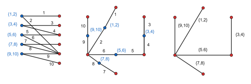
Figure 1: The tree $T_{\pi}$ (left and center) and the tree $\hat{T}_{\pi}$ (right) for the partition $\pi=\{\{1\},\{3\},\{4,5\},\{7\},\{2,6,8,9\},\{10\}\}$.

Finally, the formula (3.13) is obtained as follows.

Proof of (3.13).

If $n>k+1$, then the coefficient of $C_{k}(Y)$ with $\lambda^{n}$, is zero by Lemma A.2. Hence it follows from (A.5) that

$$\sum_{\pi\in\mathcal{P}(n)}\left(\sum_{V\in\pi}{|V|}^{2}\right)^{k}\mu_{n}(\pi,1_{n})=\psi_{n}^{(k)}(0)=0$$

By Lemma A.2 and (A.6), the $n$-th coefficient of $C_{n-1}(Y)$ with respect to $\lambda$ equals to $2^{n-1}n^{n-3}$, and therefore it follows from (A.5) that

$$\sum_{\pi\in\mathcal{P}(n)}\left(\sum_{V\in\pi}{|V|}^{2}\right)^{n-1}\mu_{n}(\pi,1_{n})=\psi_{n}^{(n-1)}(0)=2^{n-1}n!n^{n-3}=2^{n-1}(n-1)!n^{n-2}.$$

∎

Appendix B Free cumulants via Lagrange inversion theorem

In this appendix, we compute the free cumulants of free unitary normal distribution $\sigma_{t}$ and free unitary Poisson distribution $\Pi_{t}$ appeared in Section 6. A calculation strategy is use of the Lagrange inversion theorem (see, e.g., [9, p. 148, Theorem A]).

Recall that, for a probability measure $\mu$ (on $[0,\infty)$ or $\mathbb{T})$ with nonzero first moment, we obtain

$$R_{\mu}(zS_{\mu}(z))=z$$

on a neighborhood of $0$, where $R_{\mu}(z)$ is the R-transform of $\mu$ and $S_{\mu}(z)$ is the S-transform of $\mu$, see [4, 5] for details. If $f_{\mu}(z):=zS_{\mu}(z)$ is analytic on a neighborhood of $0$ and $f_{\mu}(0)=0$ and also $f_{\mu}^{\prime}(0)\neq 0$, then the Lagrange inversion theorem implies that

$$\kappa_{n}(\mu)=\frac{1}{n!}\lim_{z\rightarrow 0}\left(\frac{d}{dz}\right)^{n-1}\left(\frac{z}{f_{\mu}(z)}\right)^{n}.$$

B.1 Free unitary normal distribution

We give a strict written proof of the following known result by the above strategy.

Proposition B.1 (see [10]).

For $n\in\mathbb{N}$ and $t>0$, we have

$$\kappa_{n}(\sigma_{t})=\exp\left(-\frac{nt}{2}\right)\frac{(-nt)^{n-1}}{n!}.$$

Proof.

Recall that, for any $t>0$,

$$S_{\sigma_{t}}(z)=\exp\left(t\left(z+\frac{1}{2}\right)\right).$$

Then it is easy to verify that $f_{\sigma_{t}}(z):=zS_{\sigma_{t}}(z)$ is analytic on a neighborhood of $0$ and $f_{\sigma_{t}}(0)=0$ and also $f_{\sigma_{t}}^{\prime}(0)=e^{t/2}\neq 0$. The Lagrange inversion theorem implies that

$$\kappa_{n}(\sigma_{t}) =\frac{1}{n!}\lim_{z\rightarrow 0}\left(\frac{d}{dz}\right)^{n-1}\left(\frac{z}{f_{\sigma_{t}}(z)}\right)^{n}$$

$$=\frac{1}{n!}\lim_{z\rightarrow 0}\left(\frac{d}{dz}\right)^{n-1}\exp\left(-nt\left(z+\frac{1}{2}\right)\right)$$

$$=\exp\left(-\frac{nt}{2}\right)\frac{(-nt)^{n-1}}{n!}.$$

∎

B.2 Free unitary Poisson distribution

We introduce a calculation result on the free cumulants of free unitary Poisson distribution $\Pi_{t}$.

Proposition B.2.

For $n\in\mathbb{N}$ and $t>0$, we get

$$\kappa_{n}(\Pi_{t})=(-1)^{n-1}2^{n}e^{-2nt}\sum_{k=1}^{n-1}\frac{(-t)^{k}}{k!}(2n)^{k-1}\binom{n-2}{k-1}.$$ (B.1)

To show this, we use the Lagrange inversion theorem again. According to [14], we have

$$S_{\Pi_{t}}(z)=\exp\left(\frac{t}{z+\frac{1}{2}}\right),\qquad t>0.$$

One can see that, $f_{\Pi_{t}}(z)=zS_{\Pi_{t}}(z)$ is analytic on a neighborhood of $0$, and $f_{\Pi_{t}}(0)=0$ and also $f_{\Pi_{t}}^{\prime}(0)=e^{2t}\neq 0$. By the Lagrange inversion theorem, we have

$$\begin{split}\kappa_{n}(\Pi_{t})&=\frac{1}{n!}\lim_{z\rightarrow 0}\frac{d^{n-1}}{dz^{n-1}}\left(\frac{z}{f_{\Pi_{t}}(z)}\right)^{n}\\ &=\frac{1}{n!}\lim_{z\rightarrow 0}\frac{d^{n-1}}{dz^{n-1}}\exp\left(\frac{-nt}{z+\frac{1}{2}}\right).\end{split}$$ (B.2)

The rest of computation is the above $(n-1)$-th derivative. To do it, we prepare the following result derived from the Faá Di Bruno’s formula.

Lemma B.3.

Let $u$ be an analytic function on $\mathbb{C}$. Then

$$\frac{d^{n}}{dz^{n}}e^{u(z)}=\left(\sum_{\pi\in\mathcal{P}(n)}\prod_{V\in\pi}u^{(|V|)}(z)\right)e^{u(z)}.$$

Proof.

According to the Faá Di Bruno’s formula, for analytic functions $f$ and $g$, we have

$$\frac{d^{n}}{dz^{n}}f(g(z))=\sum_{\pi\in\mathcal{P}(n)}f^{(|\pi|)}(g(z))\cdot\prod_{V\in\pi}g^{(|V|)}(z).$$

Taking $f(z)=e^{z}$ and $g(z)=u(z)$, and observing that $f^{(|\pi|)}(z)=e^{z}$, the desired result follows. ∎

The complete computation is as follows.

Proof of Proposition B.2.

By (B.2) and Lemma B.3, we obatin

$$\kappa_{n}(\Pi_{t}) =\frac{1}{n!}(-2)^{n-1}e^{-2nt}\left(\sum_{\pi\in\mathcal{P}(n-1)}(-2nt)^{|\pi|}\prod_{V\in\pi}|V|!\right)$$

$$=\frac{1}{n!}(-2)^{n-1}e^{-2nt}\left(\sum_{k=1}^{n-1}(-2nt)^{k}\sum_{\begin{subarray}{c}\pi\in\mathcal{P}(n-1)\\ |\pi|=k\end{subarray}}\prod_{V\in\pi}|V|!\right)$$

$$=(-1)^{n-1}2^{n}e^{-2nt}\left(\sum_{k=1}^{n-1}(-t)^{k}(2n)^{k-1}\sum_{\begin{subarray}{c}\pi\in\mathcal{P}(n-1)\\ |\pi|=k\end{subarray}}\frac{\prod_{V\in\pi}|V|!}{(n-1)!}\right).$$

Hence, it is enough to prove

$$\sum_{\begin{subarray}{c}\pi\in\mathcal{P}(n-1)\\ |\pi|=k\end{subarray}}\frac{\prod_{V\in\pi}|V|!}{(n-1)!}=\frac{1}{k!}\binom{n-2}{k-1}$$

by comparing with (B.1). Note that the elementary combinatorics shows that

$$\sum_{\begin{subarray}{c}p_{1},\dots,p_{n-1}\geq 0\\ p_{1}+\cdots+(n-1)p_{n-1}=n-1\\ p_{1}+\cdots+p_{n-1}=k\end{subarray}}\binom{k}{p_{1},\dots,p_{n-1}}=\binom{n-2}{k-1},\qquad 1\leq k\leq n-1.$$ (B.3)

Thus, since the number of partitions with $p_{1}$ blocks of size $1$, $p_{2}$ blocks of size $2$,$\dots$, $p_{n}$ blocks of size $n$ is equal to

$$\frac{n!}{p_{1}!p_{2}!\cdots p_{n}!(1!)^{p_{1}}(2!)^{p_{2}}\cdots(n!)^{p_{n}}},$$

we have

$$\sum_{\begin{subarray}{c}\pi\in\mathcal{P}(n-1)\\ |\pi|=k\end{subarray}}\frac{\prod_{V\in\pi}|V|!}{(n-1)!} =\frac{1}{k!}\sum_{\begin{subarray}{c}p_{1},\dots,p_{n-1}\geq 0\\ p_{1}+\cdots+(n-1)p_{n-1}=n-1\\ p_{1}+\cdots+p_{n-1}=k\end{subarray}}\binom{k}{p_{1},\dots,p_{n-1}}$$

$$=\frac{1}{k!}\binom{n-2}{k-1},$$

where the last equality follows from (B.3). ∎

1. Octavio Arizmendi
   Centro de Investigación en Matemáticas, Guanajuato, Gto. 36000, Mexico.
   Email: octavius@cimat.mx

2. Katsunori Fujie
   Department of Mathematics, Hokkaido University. North 10 West 8, Kita-Ku, Sapporo, Hokkaido, 060-0810, Japan.
   Email: kfujie@eis.hokudai.ac.jp

3. Yuki Ueda
   Department of Mathematics, Hokkaido University of Education. Hokumon-cho 9, Asahikawa, Hokkaido, 070-8621, Japan.
   Email: ueda.yuki@a.hokkyodai.ac.jp

References

- [1] O. Arizmendi, J. Garza-Vargas and D. Perales, Finite Free Cumulants: Multiplicative Convolutions, Genus Expansion and Infinitesimal Distributions. arXiv:2108.08489.
- [2] O. Arizmendi and D. Perales, Cumulants for finite free convolution. J. Combin. Theory Ser. A 155 (2018), 244–266.
- [3] O. Arizmendi and C. Vargas, Products of free random variables and -divisible non-crossing partitions. Electron. Commun. Probab. 17 (2012), 1–13.
- [4] H. Bercovici and D. Voiculescu. Lévy-Hincin type theorems for multiplicative and additive free convolution. Pacific J. Math., 153, no.2, (1992), 217–248.
- [5] H. Bercovici and D. Voiculescu, Free convolution of measures with unbounded support. Indiana Univ. Math. J. 42 (1993), 733–773.
- [6] P. Biane. Free Brownian motion, free stochastic calculus and random matrices. In Free probability theory (Waterloo, ON, 1995), volume 12 of Fields Inst. Commun., Pages 1–19. Amer. Math. Soc., Providence, RI.
- [7] P. Biane. Segal-Bargmann transform, functional calculus on matrix spaces and the theory of semi-circular and circular systems. J. Funct. Anal., 144, no.1, (1997), 232–286.
- [8] G. Cébron. Matricial model for the free multiplicative convolution. Ann. Probab., 44, no.4 (2016), 2427–2478.
- [9] L. Comtet. Advanced combinatorics. D. Reidel Publishing Co., Dordrecht, enlarged edition, 1974. The art of finite and infinite expansions.
- [10] N. Demni, M. Guay-Paquet and A. Nica. Star-cumulants of free unitary Brownian motion. Adv. Appl. Math. 69 (2015), 1–45.
- [11] K. Fujie and Y. Ueda, Law of large numbers for finite free multiplicative convolution of polynomials. SIGMA 19 (2023), 004, 11 pages.
- [12] U. Haagerup and S. Möller. Tha law of large numbers for the free multiplicative convolution. Operator algebra and dynamics, 157–186, Springer Proc. Math. Stat., 58, Springer, Heidelberg, 2013.
- [13] G. H. Hardy, J. E. Littlewood and G. Poĺya. Inequalities. Cambridge at the university press. 1934.
- [14] Z. Kabluchko, Repeated differentiation and free unitary Poisson processes, arXiv:2112.14729.
- [15] Z. Kabluchko, Lee-Yang zeroes of the Curie-Weiss ferromagnet, unitary Hermite polynomials, and the backward heat flow, arXiv:2203.05533.
- [16] V. P. Leonov and A. N. Sirjaev. On a method of semi-invariants. Theor. Probability Appl., 4:319–329, 1959.
- [17] H. Maassen, Addition of freely independent random variables. J. Funct. Anal. 106 (1992), 409–438.
- [18] A. W. Marcus, Polynomial convolutions and (finite) free probability. arXiv:2108.07054.
- [19] A. W. Marcus, D. A. Spielman and N. Srivastava, Finite free convolutions of polynomials. Probab. Theory Relat. Fields 182 (2022), no. 3–4, 807–848.
- [20] M. Marden, Geometry of polynomials, 2nd edn. Number 3. American Mathematical Society, 1966.
- [21] J. A. Mingo and R. Speicher, Free probability and random matrices, Fields Institute Monographs, vol. 35, Springer, New York; Fields Institute for Research in Mathematical Sciences, Toronto, ON, 2017.
- [22] B. Mirabelli, Hermitian, Non-Hermitian and Multivariate Finite Free Probability. 2021. URL https://dataspace.princeton.edu/handle/88435/dsp019593tz21r. PhD Thesis, Princeton University.
- [23] A. Nica and R. Speicher, Lectures on the Combinatorics of Free Probability Theory, London Mathematical Society Lecture Note Series, vol. 335, Cambridge University Press, Cambridge, 2006.
- [24] N. Sakuma and H. Yoshida, New limit theorems related to free multiplicative convolution. Studia Math. 214 (2013), no.3, 251–264.
- [25] G. Szeg̈o. Bemerkungen zu einem Satz von J. H. Grace über die Wurzeln algebraischer Gleichungen, Math. Z. 13 (1), 28–55, 1922.
- [26] E. G.F. Thomas, A polarization identity for multilinear maps, Indagationes Mathematicae 25, Issue 3 (2014), 468–474
- [27] D. Voiculescu, K. J. Dykema and A. Nica, Free random variables. Number 1. American Mathematical Soc., 1992.
- [28] D. Voiculescu, Addition of certain noncommuting random variables. J. Funct. Anal. 66 (1986), 323–346 .
- [29] J. Yancey, Edge-labelled trees, Pi Mu Epsilon Journal, Vol. 8, No. 2 (1985), 96–102.
- [30] P. Zhong. Free Brownian motion and free convolution semigroups: multiplicative case. Pacific J. Math., 269, no.1 (2014), 219–256.
- [31] P. Zhong. On the free convolution with a free multiplicative analogue of the normal distribution. J. Theoret. Probab., 28, no.4 (2015), 1354–1379.