Delivering Arbitrary-Modal Semantic Segmentation

Abstract

Multimodal fusion can make semantic segmentation more robust. However, fusing an arbitrary number of modalities remains underexplored. To delve into this problem, we create the DeLiVER arbitrary-modal segmentation benchmark, covering Depth, LiDAR, multiple Views, Events, and RGB. Aside from this, we provide this dataset in four severe weather conditions as well as five sensor failure cases to exploit modal complementarity and resolve partial outages. To make this possible, we present the arbitrary cross-modal segmentation model CMNeXt. It encompasses a Self-Query Hub (SQ-Hub) designed to extract effective information from any modality for subsequent fusion with the RGB representation and adds only negligible amounts of parameters (${\sim}0.01M$) per additional modality. On top, to efficiently and flexibly harvest discriminative cues from the auxiliary modalities, we introduce the simple Parallel Pooling Mixer (PPX). With extensive experiments on a total of six benchmarks, our CMNeXt achieves state-of-the-art performance on the DeLiVER, KITTI-360, MFNet, NYU Depth V2, UrbanLF, and MCubeS datasets, allowing to scale from $1$ to $81$ modalities. On the freshly collected DeLiVER, the quad-modal CMNeXt reaches up to $66.30\%$ in mIoU with a ${+}9.10\%$ gain as compared to the mono-modal baseline.

1 Introduction

With the explosion of modular sensors, multimodal fusion for semantic segmentation has progressed rapidly recently [5, 11, 49] and in turn has stirred growing interest to assemble more and more sensors to reach higher and higher segmentation accuracy aside from more robust scene understanding. However, most works [35, 77, 107] and multimodal benchmarks [30, 62, 95] focus on specific sensor pairs, which lack behind the current trend of fusing more and more modalities [72, 4], i.e., progressing towards Arbitrary-Modal Semantic Segmentation (AMSS).

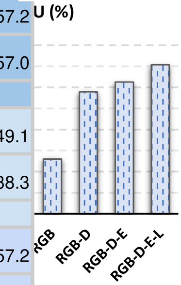
(a) RGB-D-E-L fusion.

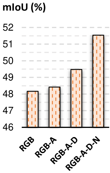
(b) RGB-A-D-N fusion.

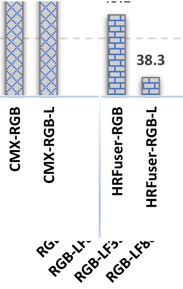
(c) RGB-Light Field.

Figure 1: Arbitrary-modal segmentation results of CMNeXt using:
(a). {RGB, Depth, Event, LiDAR} on our DeLiVER dataset; (b). {RGB, Angle of Linear Polarization (AoLP), Degree of Linear Polarization (DoLP), Near-Infrared (NIR)} on MCubeS [45]; (c). {RGB, 8/33/80 sub-aperture Light Fields (LF8/LF33/LF80) on UrbanLF-Syn [60], respectively.

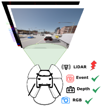
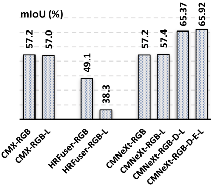
Figure 2: Comparing CMX [49], HRFuser [4], and our CMNeXt in sensor failure (i.e., LiDAR Jitter) on the DeLiVER dataset.

When looking into AMSS, two observations become apparent. Firstly, an increasing amount of modalities should provide more diverse complementary information, monotonically increasing segmentation accuracy. This is directly supported by our results when incrementally adding and fusing modalities as illustrated in Fig. 1 (RGB-Depth-Event-LiDAR), Fig. 1 (RGB-AoLP-DoLP-NIR), and Fig. 1 when adding up to $80$ sub-aperture light-field modalities (RGB-LF$8$/-LF$33$/-LF$80$). Unfortunately, this great potential cannot be uncovered by previous cross-modal fusion methods [9, 79, 103], which follow designs for pre-defined modality combinations. The second observation is that the cooperation of multiple sensors is expected to effectively combat individual sensor failures. Most of the existing works [74, 78, 69] are built on the assumption that each modality is always accurate. Under partial sensor faults, which are common in real-life robotic systems, e.g. LiDAR Jitter, fusing misaligned sensing data might even degrade the segmentation performance, as depicted with CMX [49] and HRFuser [4] in Fig. 2. These two critical observations remain to a large extent neglected.

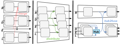
(a) Separate

(b) Joint

(c) Asymmetric

Figure 3: Comparison of multimodal fusion paradigms, such as (a) merging with separate branches [4], (b) distributing with a joint branch [72], and (c) our hub2fuse with asymmetric branches.

To address these challenges, we create a benchmark based on the CARLA simulator [19], with Depth, LiDAR, Views, Events, and RGB images: The DeLiVER Multimodal dataset. It features severe weather conditions and five sensor failure modes to exploit complementary modalities and resolve partial sensor outages. To profit from all this, we present the arbitrary cross-modal CMNeXt segmentation model. Without increasing the computation overhead substantially when adding more modalities CMNeXt incorporates a novel Hub2Fuse paradigm (Fig. 3). Unlike relying on separate branches (Fig. 3) which tend to be computationally costly or using a single joint branch (Fig. 3) which often discards valuable information, CMNeXt is an asymmetric architecture with two branches, one for RGB and another for diverse supplementary modalities.

The key challenge lies in designing the two branches to pick up multimodal cues. Specifically, at the hub step of Hub2Fuse, to gather useful complementary information from auxiliary modalities, we design a Self-Query Hub (SQ-Hub), which dynamically selects informative features from all modality-sources before fusion with the RGB branch. Another great benefit of SQ-Hub is the ease of extending it to an arbitrary number of modalities, at negligible parameters increase (${\sim}0.01M$ per modality). At the fusion step, fusing sparse modalities such as LiDAR or Event data can be difficult to handle for joint branch architectures without explicit fusion such as TokenFusion [72]. To circumvent this issue and make best use of both dense and sparse modalities, we leverage cross-fusion modules [49] and couple them with our proposed Parallel Pooling Mixer (PPX) which efficiently and flexibly harvests the most discriminative cues from any auxiliary modality. These design choices come together in our CMNeXt architecture, which paves the way for AMSS (Fig. 1). By carefully putting together alternative modalities, CMNeXt can overcome individual sensor failures and enhances segmentation robustness (Fig. 2).

With comprehensive experiments on DeLiVER and five additional public datasets, we gather insight into the strength of the CMNeXt model. On DeLiVER, CMNeXt obtains $66.30\%$ in mIoU with a ${+}9.10\%$ gain compared to the RGB-only baseline [80]. On UrbanLF-Real [60] and MCubeS [45] datasets, CMNeXt surpasses the previous best methods by ${+}3.90\%$ and ${+}8.68\%$, respectively. Compared to previous state-of-the-art methods, our model achieves comparable perfomance on bi-modal NYU Depth V2 [62] as well as MFNet [30] and outperforms all previous modality-specific methods on KITTI-360 [46].

On a glance, we deliver the following contributions:

• We create the new benchmark DeLiVER for Arbitrary-Modal Semantic Segmentation (AMSS) with four modalities, four adverse weather conditions, and five sensor failure modes.

• We revisit and compare different multimodal fusion paradigms and present the Hub2Fuse paradigm with an asymmetric architecture to attain AMSS.

• The universal arbitrary cross-modal fusion model CMNeXt is proposed, with a Self-Query Hub (SQ-Hub) for selecting informative features and a Parallel Pooling Mixer (PPX) for harvesting discriminative cues.

• We investigate AMSS by fusing up to a total of $80$ modalities and notice that CMNeXt achieves state-of-the-art performances on six datasets.

2 Related Work

Semantic segmentation has experienced striking progress since fully convolutional networks [52] introducing the end-to-end per-pixel classification paradigm, which was enhanced by capturing multi-scale features [7, 8, 33, 97], appending channel- and self-attention blocks [14, 21, 36, 89], refining context priors [37, 47, 85, 93], and leveraging edge cues [3, 17, 42, 67]. Recently, with the application of vision transformers in recognition tasks, dense prediction transformers [18, 40, 71, 88] and semantic segmentation transformers [26, 64, 91, 98] emerge, along with the mask classification paradigm [13, 12] to jointly handle things and stuff segmentation. Following the general architecture of transformers, attention-based token mixing has been substituted with MLP-based [10, 32, 44], pooling [86], and convolutional [27, 28] blocks. While these works achieve great improvements on mainstream image segmentation benchmarks, they still suffer under real-world conditions where RGB images do not offer sufficient textures like low-illumination and fast-moving scenarios.

Multimodal semantic segmentation has been considered by harvesting complementary features from supplementary modalities such as depth [5, 9, 84, 100], thermal [61, 75, 96], polarization [39, 54, 79], events [1, 95], LiDAR [83, 107], and optical flow [57]. To scale from modality-specific fusion to unified fusion, CMX [49] tackles RGB-X segmentation with multi-level cross-modal interactions, whereas channel- and token exchanges are explored in [72, 73, 74]. Additional multimodal fusion methods address object detection [43, 63], medical and material segmentation [45, 81], as well as flow estimation [48]. Most of these works focus on fusing complementary cues, but they do not fully consider multimodal learning in scenarios where some modalities fail. To this end, we propose CMNeXt, a universal multimodal semantic segmentation framework with arbitrary-modal complements. Unlike previous modality-specific fusion methods [35, 54, 95], CMNeXt scales from bi-modal scenarios like RGB-D parsing to arbitrary-modal fusion like light field segmentation with virtually $81$ modalities. In addition, we provide a DeLiVER benchmark to foster multimodal learning. While there are some existing datasets [24, 59, 68] based on the CARLA simulator [19], our dataset not only provides diverse sensing data but also sensor-failure cases for robust semantic understanding.

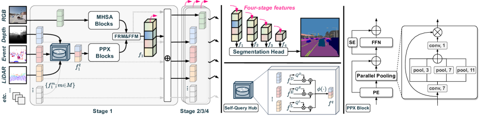
Figure 4: CMNeXt architecture in Hub2Fuse paradigm and asymmetric branches, having e.g. Multi-Head Self-Attention (MHSA) [80] blocks in the RGB branch and our Parallel Pooling Mixer (PPX) blocks in the accompanying branch. At the hub step, the Self-Query Hub selects informative features from the supplementary modalities. At the fusion step, the feature rectification module (FRM) and feature fusion module (FFM) [49] are used for feature fusion. Between stages, features of each modality are restored via adding the fused feature. The four-stage fused features are forwarded to the segmentation head for the final prediction.

3 CMNeXt: Proposed Framework

To achieve arbitrary-modal segmentation, the proposed CMNeXt framework is constructed by using a dual-branch structure in a Hub2Fuse paradigm. We will elaborate the overall CMNeXt architecture in Sec. 3.1, the Self-Query Hub in Sec. 3.2, and the Parallel Pooling Mixer in Sec. 3.3.

3.1 CMNeXt Architecture

In Fig. 4, our CMNeXt has an encoder-decoder architecture. The encoder is a dual-branch and four-stage encoder. Built on the assumption that the RGB representation is essential for semantic segmentation, the two branches correspond to the primary branch for RGB and the secondary branch for other modalities, respectively. The four-stage structure follows most of previous CNN/Transformer models [97, 21, 80, 71] to extract pyramidal features. Note that, Fig. 4 details only the first of the four stages for brevity. For the consistency of modal representations, we preprocess LiDAR and Event data as image-like representations following [107, 95]. The RGB image $\bm{I}_{RGB}{\in}H{\times}W{\times}3$ is gradually processed by Multi-Head Self-Attention (MHSA) blocks [80], whereas the images of the other $M$ modalities $\bm{I}_{M}{\in}H{\times}W{\times}3{\times}M$ by Parallel Pooling Mixer (PPX) blocks. After four stages, there are $M{+}1$ sets of four-stage feature maps $\bm{f}_{l}^{m}{\in}\{\bm{f}_{1}^{m},\bm{f}_{2}^{m},\bm{f}_{3}^{m},\bm{f}_{4}^{m}\}$, $m{\in}[1,M{+}1]$. In the $l^{th}$ stage, the block number of each branch is $b_{l}{\in}\{4,8,16,32\}$, the stride is $s_{l}{\in}\{4,8,16,32\}$, and the channel dimension is $C_{l}{\in}\{64,128,320,512\}$. Inside each stage, $M{+}1$ features are processed in the Hub2Fuse paradigm: At the hub step, $M$ feature maps will be merged into one feature $\bm{f}^{q}$ via the proposed Self-Query Hub. At the fusion step, the merged feature $\bm{f}^{q}$ will be further fused with RGB feature by the cross-modal Feature Rectification Module (FRM) [49] and Feature Fusion Module (FFM) [49], termed as $\bm{f}$. These two modules enable better multimodal feature fusion and interaction, and are crucial when fusing RGB with sparse features, which will be shown in our experiments. Between stages, $M{+}1$ feature maps will be restored via adding the fused feature $\bm{f}$, respectively. After the encoder, the four-stage features $\bm{f_{l}}{\in}\{\bm{f}_{1},\bm{f}_{2},\bm{f}_{3},\bm{f}_{4}\}$ will be forwarded to the decoder for the segmentation prediction. We use the MLP decoder [80] as the segmentation head.

3.2 Self-Query Hub

To perform arbitrary-modal fusion, the Self-Query Hub (SQ-Hub) is a crucial design to select the informative features of supplementary modalities before fusing with the RGB feature. As shown in Fig. 4, given a set of $M$ supplementary features $\{\bm{f}^{m}|m{\in}[1,M],\bm{f}^{m}{\in}H{\times}W{\times}C\}$, a Self-Query module is applied to calculate the informative score mask $Q^{m}{\in}H{\times}W$ of each feature $\bm{f}^{m}$, as in Eq. (1) and (2).

$$\begin{split}\bm{\hat{f}}^{m}&=\text{DW-Conv}_{3{\times}3}{(C,C)}(\bm{f}^{m}),\end{split}$$ (1)

$$\begin{split}Q^{m}&=\text{Sigmoid}(\text{Conv}(C,1)(\bm{\hat{f}}^{m})),\end{split}$$ (2)

where the $\text{DW-Conv}_{3{\times}3}{(C_{in},C_{out})}(\cdot)$ means a Depth-Wise convolution layer with a kernel size of $3{\times}3$. After obtaining $M$ score masks through $M$ respective self-query modules, a cross-modal comparison is conducted between $M$ features $\{\bm{f}^{m}|m{\in}[1,M]\}$. That is, each patch $p^{q}$ of the merged feature map $\bm{f}^{q}$ will be filled by the patch $p^{m}$ of $\{\bm{f}^{m}|m{\in}[1,M]\}$ with the highest score, i.e., the most effective patch among $M$ modalities. It can be formalized as:

$$\begin{split}\bm{f}^{q}&=\{p^{q}|p^{q}{\in}{H{\times}W}\}\\ &=\phi(\{\bm{f}^{m}{+}Q^{m}{\cdot}\bm{\hat{f}}^{m}|m{\in}[1,M]\})\\ &=\phi(\{p^{m}|p^{m}{\in}{H{\times}W},m{\in}[1,M]\}),\end{split}$$ (3)

where $\phi(\cdot)$ is an operation to select the maximum $p^{m}$ from $\{\bm{f}^{m}{+}Q^{m}{\cdot}\bm{\hat{f}}^{m}|m{\in}[1,M]\}$. Then, the merged feature $\bm{f}^{q}$ is forwarded to the Parallel Pooling Mixer (PPX).

3.3 Parallel Pooling Mixer

Another crucial design in CMNeXt is the Parallel Pooling Mixer (Fig. 4), which is proposed to efficiently and flexibly harvest discriminative cues from arbitrary-modal complements in the aforementioned SQ-Hub. Given the merged feature map $\bm{f}^{q}{\in}H{\times}W{\times}C$ from SQ-Hub, a $7{\times}7$ DW-Conv layer is applied to aggregate local information. The three parallel pooling layers are for capturing multi-scale modal features, which will be summed with the residual one and mixed by a $1{\times}1$ convolution. Then, a Sigmoid function is used to calculate the attention for weighting. The first part of PPX can be written as:

$$\begin{split}\hat{\bm{f}^{q}}&=\text{DW-Conv}_{7{\times}7}(C,C)(\bm{f}^{q}),\end{split}$$ (4)

$$\begin{split}\hat{\bm{f}^{q}}&\coloneqq\sum_{k{\in}\{3,7,11\}}\text{Pool}_{k{\times}k}(\hat{\bm{f}^{q}})+\hat{\bm{f}^{q}},\end{split}$$ (5)

$$\begin{split}\bm{w}&=\text{Sigmoid}(\text{Conv}_{1{\times}1}(C,C)(\hat{\bm{f}^{q}})),\end{split}$$ (6)

$$\begin{split}\bm{f}^{w}&=\bm{w}{\cdot}\bm{f}^{q}+\bm{f}^{q}.\end{split}$$ (7)

Previous cross-modal fusion methods show that channel information is crucial [11, 35]. Inspired by this, we apply a Squeeze-and-Excitation (SE) module [34] in the mixing part of PPX. This structure is crucial since some channels of certain modalities do capture more significant information than others. It can further engage more spatially-holistic knowledge in the channels of the cross-modal complements in SQ-Hub. Thus, the weighted feature $\bm{f}^{w}$ is passed to a Feed-Forward Network (FFN) and a SE module [34] for enhancing the channel information. The second part of PPX can be written as:

$$\hat{\bm{f}^{w}} =\text{FFN}(C,C)(\bm{f}^{w})+\text{SE}(\bm{f}^{w}).$$ (8)

After the PPX block, $\hat{\bm{f}^{w}}$ is fused with RGB feature to form the final fused feature $\bm{f_{l}}{\in}\{\bm{f}_{1},\bm{f}_{2},\bm{f}_{3},\bm{f}_{4}\}$ by using FRM&FFM modules [49], as shown in Fig. 4.

Compared with convolution-based MSCA [27], pooling-based MetaFormer [86], fully-attentional FAN [99], our PPX includes two advances: (1) parallel pooling layers for efficient weighting in the attention part; (2) channel-wise enhancement in the feature mixing part. Both characteristics of the PPX block help in highlighting the cross-modal fused feature spatial- and channel-wise, respectively. More comparisons will be presented in Section 5.

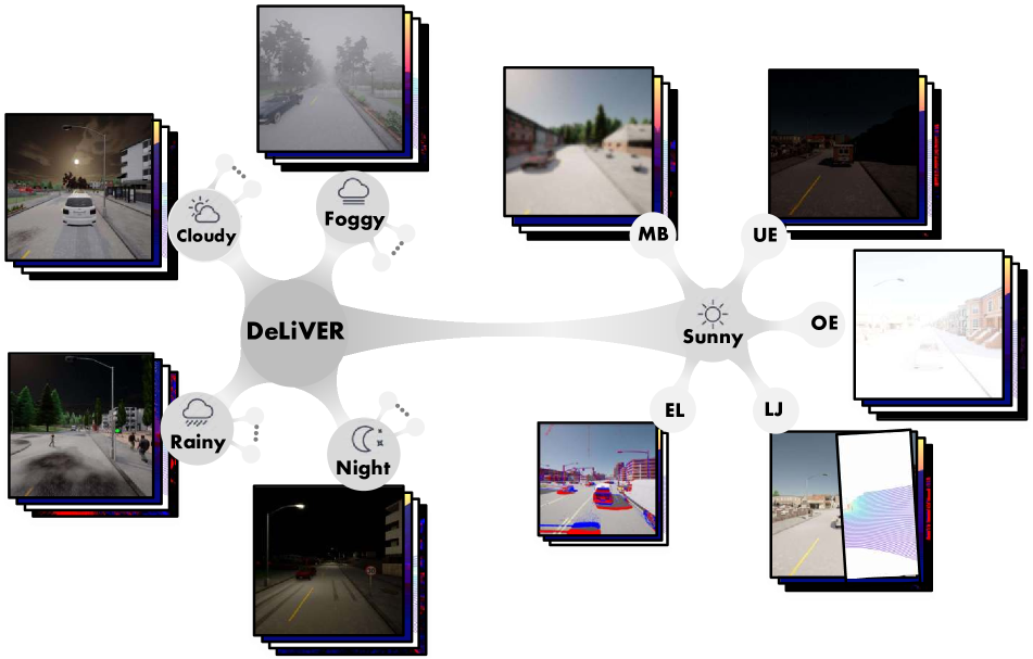
(a) Structure and samples of four adverse conditions and five failure cases.

(b) Statistic of different data splits and views.

Split	Cloudy	Foggy	Night	Rainy	Sunny	Normal	Corner	Total
Train	794	795	797	799	798	2585	1398	3983
Val	398	400	410	398	399	1298	707	2005
Test	379	379	379	380	380	1198	699	1897
Front-view	1571	1574	1586	1577	1577	5081	2804	7885
All six views	9426	9444	9516	9462	9462	30486	16824	47310

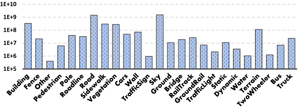
(c) Distribution of $25$ semantic classes in logarithmic scaling.

Figure 5: DeLiVER multimodal dataset including (a) four adverse conditions out of five conditions(i.e., cloudy, foggy, night-time, rainy and sunny). Apart from normal cases, each condition has five corner cases (i.e., MB: Motion Blur; OE: Over-Exposure; UE: Under-Exposure; LJ: LiDAR-Jitter; and EL: Event Low-resolution). Each sample has six views. Each view has four modalities and two labels (i.e., semantic and instance). (b) is the data statistics. (c) is the data distribution of $25$ semantic classes.

4 The DeLiVER Multimodal Dataset

Sensor settings and modalities. As presented in Fig. 5, we spent the effort to create a large-scale multimodal segmentation dataset DeLiVER with Depth, LiDAR, Views, Event, RGB data, based on the CARLA simulator [19]. DeLiVER provides six mutually orthogonal views (i.e., front, rear, left, right, up, down) of the same spatial viewpoint, i.e., a complete frame of data is encoded in the format of a panoramic cubemap. The Field-of-View (FoV) of each view is $91^{\circ}{\times}91^{\circ}$ and the image resolution is $1042{\times}1042$. All Depth, Views, and Event sensors use the same camera settings when the sensor is working properly. According to the characteristics of recent LiDAR sensors [23], we further customize a $64$ vertical channels virtual semantic LiDAR sensor to generate a point cloud of $1,728,000$ points per second with a FoV of $360^{\circ}{\times}(-30^{\circ}{\sim}10^{\circ})$ and a range of $100$ meters, so as to collect relatively dense LiDAR data.

Adverse conditions and corner cases. In addition to the multimodal setup, DeLiVER provides cases in two-fold, including four environmental conditions and five partial sensor failure cases (Fig. 5(a)). For environmental conditions, we consider cloudy, foggy, night, and rainy weather conditions other than only sunny days. The environmental conditions will cause variations in the position and illumination of the sun, atmospheric diffuse reflections, precipitation, and shading of the scene, introducing challenges for robust perception. For sensor failure cases, we consider Motion Blur (MB), Over-Exposure (OE), and Under-Exposure (UE) common for RGB cameras. LiDAR failures usually manifest as along-axis LiDAR-Jitter (LJ) due to fixation issues or rotational axis eccentricity, thus we add random angular jitters in the range of $[-1^{\circ},1^{\circ}]$ and position jitters of $[-1cm,1cm]$ to the three axial directions of the LiDAR sensor. Due to the circuit design, the resolution of the currently-used event sensors is limited [22]. Thus, we customize an Event Low-resolution (EL) scenario with $0.25{\times}$ resolution for the event camera to simulate actual devices.

Statistics and annotations. Including six views, DeLiVER has totally $47,310$ frames (Fig. 5(b)) with the size of $1042{\times}1042$. The $7,885$ front-view samples are divided into $3,983/2,005/1,897$ for training/validation/testing, respectively, each of which contains two types of annotations (i.e., semantic and instance segmentation labels). Note that, we mainly discuss the front view and the semantic segmentation task in this work, while other views and instance segmentation will be future works. To improve the class diversity of annotations ($25$ classes as in Fig. 5(c)), we modify and remap the semantic labels in the source code. Specifically, the Vehicles class is subdivided into four fine-grained categories: Cars, TwoWheeler, Bus, and Truck for both the semantic camera and the semantic LiDAR, making DeLiVER compatible with popular segmentation datasets.

5 Experiments

5.1 Datasets and Implementation Details

KITTI-360 [46] is a suburban driving dataset, having $49,004/12,276$ images at the size of $1408{\times}376$ for training/validation with $19$ classes. To study RGB-Depth-Event-LiDAR fusion consistent with the DeLiVER dataset, we generate depth images and event data by using popular off-the-shelf models, i.e., AANet [82] and EventGAN [105].

MFNet [30] is an urban street dataset with $1,569$ RGB-Thermal pairs at the size of $640{\times}480$ with $8$ classes. $820$ pairs are collected during the day and the other $749$ are captured at night. The training set consists of $50\%$ of the daytime- and $50\%$ of the nighttime images, whereas the validation- and test set respectively contains $25\%$ of the daytime- and $25\%$ of the nighttime images.

NYU Depth V2 [62] is an indoor understanding dataset with $1,449$ RGB-Depth pairs at the size of $640{\times}480$, splitting into $795/654$ for training/testing with $40$ classes.

UrbanLF [60] is a light field semantic segmentation dataset with both real-world and synthetic sets annotated in $14$ classes, respectively splitting into $580/80/164$ and $172/28/50$ samples for training/validation/testing. The real images have a size of $623{\times}432$, whereas the synthetic ones are of $640{\times}480$. Each sample is composed of $81$ sub-aperture images, leading to $81$ modalities.

MCubeS [45] is a dataset with pairs of RGB, Near-Infrared (NIR), Degree of Linear Polarization (DoLP), and Angle of Linear Polarization (AoLP), to study semantic material segmentation of $20$ classes. It has $302/96/102$ image pairs for training/validation/testing at the size of $1224{\times}1024$.

Implementation details. We train our models on four A100 GPUs with an initial learning rate (LR) of $6e^{-5}$, which is scheduled by the poly strategy with power $0.9$ over $200$ epochs. The first $10$ epochs are to warm-up models with $0.1{\times}$ the original LR. We use cross-entropy loss function. The optimizer is AdamW [53] with epsilon $1e^{-8}$, weight decay $1e^{-2}$, and the batch size is $2$ on each GPU. The images are augmented by random resize with ratio $0.5$–$2.0$, random horizontal flipping, random color jitter, random gaussian blur, and random cropping to $1024{\times}1024$ on DeLiVER, while to their proposed sizes on other datasets. To conduct comparisons, the ImageNet-1K [16] pre-trained weight for the accompanying branch is not used on DeLiVER and KITTI-360, while the pre-trained weight for the RGB branch is applied on all datasets.

5.2 Comparison against the State of the Art

To verify the efficacy of our proposed CMNeXt framework, we conduct extensive experiments on six multimodal segmentation datasets. The results and comparisons against the state-of-the-art are shown in Table 1.

Table 1: Results on six multimodal semantic segmentation datasets. The KITTI-360 [46] and our DeLiVER datasets have up to four modalities. The MFNet [30] and NYU Depth V2 [62] datasets are dual-modal with respective RGB-Thermal and RGB-Depth modalities. The UrbanLF [60] has up to 81 sub-aperture light-filed images. The quad-modal MCubeS dataset [45] is for material segmentation.

(a) Results on KITTI-360 and DeLiVER datasets.

Method	Modal	Backbone	KITTI-360	DeLiVER
HRFuser [4]	RGB	HRFormer-T	53.20	47.95
SegFormer [80]	RGB	MiT-B2	67.04	57.20
HRFuser [4]	RGB-Depth	HRFormer-T	49.32	51.88
TokenFusion [72]	RGB-Depth	MiT-B2	57.44	60.25
CMX [49]	RGB-Depth	MiT-B2	64.43	62.67
CMNeXt	RGB-Depth	MiT-B2	65.09	63.58
HRFuser [4]	RGB-Event	HRFormer-T	44.85	42.22
TokenFusion [72]	RGB-Event	MiT-B2	55.97	45.63
CMX [49]	RGB-Event	MiT-B2	64.03	56.52
CMNeXt	RGB-Event	MiT-B2	66.13	57.48
HRFuser [4]	RGB-LiDAR	HRFormer-T	48.74	43.13
TokenFusion [72]	RGB-LiDAR	MiT-B2	54.55	53.01
CMX [49]	RGB-LiDAR	MiT-B2	64.31	56.37
CMNeXt	RGB-LiDAR	MiT-B2	65.26	58.04
HRFuser [4]	RGB-D-Event	HRFormer-T	50.21	51.83
CMNeXt	RGB-D-Event	MiT-B2	67.73	64.44
HRFuser [4]	RGB-D-LiDAR	HRFormer-T	52.61	52.72
CMNeXt	RGB-D-LiDAR	MiT-B2	66.55	65.50
HRFuser [4]	RGB-D-E-Li	HRFormer-T	52.76	52.97
CMNeXt	RGB-D-E-Li	MiT-B2	67.84	66.30

(b) Results on MFNet.

Method	Modal	mIoU
SwinT [50]	RGB	49.0
SegFormer [80]	RGB	52.0
ACNet [35]	RGB-T	46.3
FuseSeg [66]	RGB-T	54.5
ABMDRNet [96]	RGB-T	54.8
LASNet [41]	RGB-T	54.9
FEANet [15]	RGB-T	55.3
MFTNet [101]	RGB-T	57.3
GMNet [103]	RGB-T	57.3
DooDLeNet [20]	RGB-T	57.3
CMX (MiT-B2) [49]	RGB-T	58.2
CMX (MiT-B4) [49]	RGB-T	59.7
CMNeXt (MiT-B4)	RGB-T	59.9

(c) Results on NYU Depth V2.

Method	mIoU
ACNet [35]	48.3
SGNet [9]	51.1
ShapeConv [5]	51.3
NANet [92]	52.3
SA-Gate [11]	52.4
PGDENet [104]	53.7
TokenFusion [72]	54.2
TransD-Fusion [78]	55.5
MultiMAE [2]	56.0
Omnivore [25]	56.8
CMX (MiT-B4) [49]	56.3
CMX (MiT-B5) [49]	56.9
CMNeXt (MiT-B4)	56.9

(d) Results on UrbanLF-Real and -Syn.

Method	Modal	Real	Syn
PSPNet [97]	RGB	76.34	75.78
OCR [87]	RGB	78.60	79.36
SegFormer [80] (B4)	RGB	82.20	78.53
DAVSS [106]	Video	75.91	74.27
TMANet [70]	Video	77.14	76.41
ESANet [58]	RGB-D	n.a.	79.43
SA-Gate [11]	RGB-D	n.a.	79.53
PSPNet-LF [60]	RGB-LF33	78.10	77.88
OCR-LF [60]	RGB-LF33	79.32	80.43
CMNeXt (MiT-B4)	RGB-LF8	83.22	80.74
CMNeXt (MiT-B4)	RGB-LF33	82.62	80.98
CMNeXt (MiT-B4)	RGB-LF80	83.11	81.02

(e) Results on MCubeS.

Method	Modal	mIoU
DRConv [6]	RGB-A-D-N	34.63
DDF [102]	RGB-A-D-N	36.16
TransFuser [55]	RGB-A-D-N	37.66
MMTM [38]	RGB-A-D-N	39.71
FuseNet [31]	RGB-A-D-N	40.58
MCubeSNet [45]	RGB	33.70
CMNeXt (MiT-B2)	RGB	48.16
MCubeSNet [45]	RGB-A	39.10
CMNeXt (MiT-B2)	RGB-A	48.42
MCubeSNet [45]	RGB-A-D	42.00
CMNeXt (MiT-B2)	RGB-A-D	49.48
MCubeSNet [45]	RGB-A-D-N	42.86
CMNeXt (MiT-B2)	RGB-A-D-N	51.54

Results on DeLiVER. Table 1(a) summarizes the extensive comparisons between our CMNeXt and other recent methods on DeLiVER dataset. Overall, CMNeXt sets the state of the art on the fusion of two to four modalities. While fusing RGB with Depth, Event, and LiDAR, the bi-modal CMNeXt yields sufficient improvements, compared to HRFuser [4] and TokenFusion [72]. This demonstrates the superiority of our Hub2Fuse paradigm over the seperate and joint branch paradigm (Fig. 3 and Fig. 3), especially when fusing sparse modalities, i.e., Event and LiDAR. From RGB-only to gradually fusing Depth, Events, and LiDAR, the mIoU scores of CMNeXt are gradually increased ($57.20\%{\rightarrow}63.58\%{\rightarrow}64.44\%{\rightarrow}66.30\%$), showing the advance of arbitrary-modal fusion for segmentation. Thanks to the complementary features from other modalities, our quad-modal CMNeXt outperforms the RGB-only baseline SegFormer [80] by a significant margin of ${+}9.10\%$.

Results on KITTI-360. In Table 1(a), apart from the DeLiVER dataset with adverse cases, we further conduct equivalent experiments on KITTI-360 [46] which only contains normal scenes. We found that most of the multimodal fusion methods on KITTI-360 did not bring the expected high improvement. There are two conjectures: The samples are collected in suburbs and are composed of video sequences, resulting in insufficient scene diversity; The depth- and event data are generated from RGB sequences, resulting in limited modal differences. Thus, the segmentation output relies on the RGB segmentation, and adding modalities might be redundant. Nonetheless, our quad-modal CMNeXt achieves a ${+}0.80\%$ gain compared to the RGB-only baseline [80]. Besides, our bi-modal CMNeXt performs superior to CMX [49] by ${+}1.56\%$ to ${+}2.85\%$. When fusing three to four modalities, CMNeXt has respective ${+}17.52\%$, ${+}13.94\%$, and ${+}15.08\%$ gains compared to HRFuser [4].

RGB-T and RGB-D segmentation. As shown in Table 1(b) and 1(c), we further conduct experiments on bi-modal datasets, MFNet [30] and NYU Depth V2 [62], which comprise dense thermal and depth data as supplementary information. Our CMNeXt achieves the state of the art on both datasets. Using MiT-B4 [80], CMNeXt outperforms CMX with ${+}0.2\%$ on MFNet. Besides, on the NYU Depth V2 dataset, it is comparable to CMX with MiT-B5. It proves the benefits of our PPX block in CMNeXt over the Multi-Head Self-Attention (MHSA) block used by CMX.

Light field semantic segmentation. Towards arbitrary-modal fusion for semantic segmentation, we apply CMNeXt on the UrbanLF dataset [60], in which each sample is composed of $81$ sub-aperture light field modalities. As shown in Table 1(d), CMNeXt surpasses the previous state of the art, OCR-LF [60], in both real-world and synthetic scenes, even with fewer modalities ($33{\rightarrow}8$). Due to the similarity between modalities in this dataset, it is challenging to extract diverse complementary features. Nonetheless, by fusing up to $80$ light field images, CMNeXt reaches respective $83.11\%$ and $81.02\%$ in mIoU on real and synthetic sets.

Multimodal material segmentation. To verify multimodal fusion in material recognition, we conduct experiments on the MCubeS dataset [45] which also contains four modalities. As shown in Table 1(e), our quad-modal CMNeXt exceeds other quad-modal models and attains the top performance of $51.54\%$, with a significant increase $8.68\%$ over MCubeSNet [45]. In addition, CMNeXt has incremental improvements when gradually adding AoLP, DoLP, and NIR modalities. The results on multimodal material segmentation are consistent with the ones of arbitrary-modal segmentation on our DeLiVER dataset.

5.3 Ablation Studies

Table 2: Results on adverse conditions of DeLiVER. Sensor failure cases are MB: Motion Blur; OE: Over-Exposure; UE: Under-Exposure; LJ: LiDAR-Jitter; and EL: Event Low-resolution. The number of parameters (#Params) and GFLOPs are counted in $512{\times}512$.

Model-modality	#Params(M)	GFLOPs	Cloudy	Foggy	Night	Rainy	Sunny	MB	OE	UE	LJ	EL	Mean
HRFuser-RGB	29.89	217.5	49.26	48.64	42.57	50.61	50.47	48.33	35.13	26.86	49.06	49.88	47.95
SegFormer-RGB	25.79	38.93	59.99	57.30	50.45	58.69	60.21	57.28	56.64	37.44	57.17	59.12	57.20
TokenFusion-RGB-D	26.01	54.96	50.92	52.02	43.37	50.70	52.21	49.22	46.22	36.39	49.58	49.17	49.86
CMX-RGB-D	66.57	65.68	63.70	62.77	60.74	62.37	63.14	59.50	60.14	55.84	62.65	63.26	62.66
HRFuser-RGB-D	30.46	223.0	54.80	51.48	49.51	51.55	52.12	50.92	41.51	44.00	54.10	52.52	51.88
HRFuser-RGB-D-E	31.04 (+0.57)	229.0 (+6.00)	54.04	50.83	50.88	51.13	52.61	49.32	41.75	47.89	54.65	52.33	51.83
HRFuser-RGB-D-E-L	31.61 (+0.57)	235.0 (+6.00)	56.20	52.39	49.85	52.53	54.02	49.44	46.31	46.92	53.94	52.72	52.97
CMNeXt-RGB-D	58.69	62.94	67.21	62.79	61.64	62.95	65.26	61.00	64.64	58.71	64.32	63.35	63.58
CMNeXt-RGB-D-E	58.72 (+0.03)	64.19 (+1.25)	68.28	63.28	62.64	63.01	66.06	62.58	64.44	58.73	65.37	65.80	64.44
CMNeXt-RGB-D-E-L	58.73 (+0.01)	65.42 (+1.23)	68.70	65.67	62.46	67.50	66.57	62.91	64.59	60.00	65.92	65.48	66.30
w.r.t. SegFormer-RGB			(+8.71)	(+8.37)	(+12.01)	(+8.81)	(+6.36)	(+5.63)	(+7.95)	(+22.56)	(+8.75)	(+6.36)	(+9.10)

Analysis in adverse weather conditions. In Table 2, we compare CMNeXt against mainstream multimodal fusion paradigms in different conditions including adverse weather- and partial sensor failure scenarios. It can be seen that despite being efficient, TokenFusion [72] suffers in these conditions as effective information is discarded in their token replacement. Due to the proposed SQ-Hub for selecting effective features, CMNeXt significantly improves the performance compared to the previous CMX [49] and HRFuser [4]. When fusing more modalities, HRFuser tends to induce much more overhead (${+}6.00$ GFLOPs when adding a branch), whereas CMNeXt brings great mIoU gains at only slight computation increase (${<}1.30$ GFLOPs). Compared with the RGB baseline, the full RGB-D-E-L CMNeXt overall improves the accuracy by $9.10\%$ on average for different conditions, in particular for the nighttime (${+}12.01\%$) and the rainy (${+}8.81\%$) scenarios.

Analysis in sensor failure cases. In the Event Low-resolution (EL) case of Table 2, from the fusion of RGB-D to RGB-D-E, the accuracy of HRFuser [4] is degraded, however, the one of CMNeXt is improved ($63.35\%{\rightarrow}66.11\%$). This is also observed in the case of LiDAR Jitter (LJ), where the performance of CMNeXt is increased ($65.37\%{\rightarrow}65.92\%$) by fusing from D-E to D-E-L. These results demonstrate the ability of CMNeXt to combat sensor failures, thanks to SQ-Hub for selecting informative features. Compared to the RGB baseline, CMNeXt obtains a ${+}22.56\%$ gain in the Under-Exposure (UE) case.

Table 3: Ablation study of the CMNeXt architecture.

Structure	#Params(M)	GFLOPs	mIoU(%)
CMNeXt	58.73	65.42	66.30
– without Addition	58.73	65.42	64.56 (-1.74)
– without SQ-Hub	58.70	65.36	64.41 (-1.89)
– with MSCA instead PPX	61.95	68.42	63.94 (-2.36)
– without SE in PPX	58.73	65.41	63.27 (-3.03)
– without FRM	48.71	64.79	62.71 (-3.59)
– without FRM&FFM	42.14	59.00	56.54 (-9.76)

Ablation of the CMNeXt architecture. As shown in Table 3, we ablate our CMNeXt architecture. When removing the addition operation of supplementary modalities, the performance slightly decreases. Without the SQ-Hub for dynamically harvesting complementary cues, the supplementary modalities are directly added and the mIoU declines by $1.89\%$. When using the MSCA from SegNeXt [27] instead of our PPX, the accuracy clearly drops. Ablating the SE block in PPX for channel processing incurs a mIoU downgrade of $3.03\%$, which indicates that the spatially-holistic knowledge in channels contribute a lot to the multimodal fusion. The FRM&FFM modules also play important roles in facilitating comprehensive cross-modal interactions between the RGB representation and the supplementary representation extracted via SQ-Hub. The results verify that the hub and fusion steps in our proposed Hub2Fuse paradigm are fundamental to arbitrary multimodal segmentation.

Table 4: Comparison of convolution-, pooling- and self-attention blocks in the RGB- and accompanying branch, respectively.

RGB	Accompanying	#Params(M)	GFLOPs	mIoU(%)
Branch	Branch
MHSA [80]+	MHSA [80]	66.87	68.39	62.92
	ConvNeXt [51]	56.42	59.85	63.73
	FAN [99]	68.10	69.49	63.73
	PoolFormer [86]	56.22	59.52	63.83
	$g^{n}$Conv [56]	62.04	64.83	64.06
	MSCA [27]	61.95	68.42	64.71
	P2T [76]	63.01	71.13	65.13
	PPX (ours)	58.73	65.42	66.30
PPX	+PPX (ours)	50.88	62.95	62.21
MSCA [27]		62.42	61.10	62.88
MHSA [80]		58.73	65.42	66.30

Comparison of token mixing blocks. As shown in Table 4, we first compare PPX against convolutional-, attentional, and pooling-based blocks when ported on our CMNeXt architecture as the accompanying branch for supplementary-modal features. PPX achieves the best mIoU score, while remaining highly efficient with few parameters. While the PoolFormer [86] has less parameters and GLFOPs, it is also less effective for harvesting cross-modal cues. PPX surpasses the MHSA in SegFormer [80], ConvNeXt [51], the fully attentional block in FAN [99], the $g^{n}$Conv in HorNet [56], the MSCA in SegNeXt [27]. Compared with the P2T block [76] adapting pyramid pooling in self-attention, our PPX is both more efficient and accurate, making it ideally suitable for learning complementary features towards arbitrary multimodal fusion.

After confirming that PPX block in the accompanying branch, for the RGB branch, we follow CMX [49] and use MHSA blocks from SegFormer. In spite of moderate complexity, MSHA [80]+PPX achieves higher accuracy than PPX+PPX and MSCA [27]+PPX, indicating that self-attention excels at learning from the dense RGB representation in multimodal semantic segmentation.

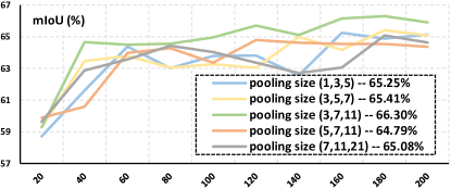
Figure 6: Training curves of different pooling sizes in PPX.

Parameter study on the pooling sizes. In Fig. 6, we investigate a variety of pooling sizes in PPX on our DeLiVER dataset, confirming the set of $\{3,7,11\}$ yields the best mIoU.

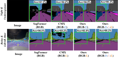
Figure 7: Visualization of segmentation results.

Visualization of arbitrary-modal segmentation. In Fig. 7, we show semantic segmentation results of our CMNeXt against the RGB-only SegFormer [80] and the RGB-X CMX [49]. It can be seen that in the dark night with under-exposure, the RGB-only SegFormer hardly segments the close vehicle, while the RGB-D CMNeXt clearly outperforms CMX. Our RGB-D-E-L CMNeXt further enhances the performance and yields more complete segmentation. In the partial sensor failure scenario with LiDAR jitter, CMX produces unsatisfactory rainy scene parsing results. Our RGB-LiDAR model is barely affected by the sensing data mis-alignment and the quad-modal CMNeXt further robustifies the full scene segmentation.

6 Conclusion

In this work, we tackle arbitrary-modal semantic segmentation. We put forward the DeLiVER multimodal dataset with four modalities and partial sensor failures under various weather conditions. We propose the Hub2Fuse paradigm with asymmetric branches and design a universal model CMNeXt for arbitrary-modal fusion with Self-Query Hub (SQ-Hub) to dynamically select complementary representations and Parallel Pooling Mixer (PPX) to efficiently and flexibly harvest discriminative cross-modal features. Our CMNeXt sets the new state of the art on six datasets, which can scale from $1$ to $81$ modalities.

Limitations. Our asymmetric architecture leverages the assumption that the RGB representation is essential for semantic segmentation, which is partially due to the fact that most pretrained weights are learned on RGB image datasets. Thus, multi-modal pretraining could be beneficial to further improve the flexibility in arbitrary-modal segmentation. Besides, while the DeLiVER dataset provides multi-view data and instance labels, only the front-view and semantics are exploited in this work. Aside from these, the fusion of 3D representations of LiDAR and Event data could be addressed in our future work based on the DeLiVER dataset.

Appendix A DeLiVER Dataset

A.1 Detailed settings in data collection

Depth2Frames. The depth camera straightforwardly outputs a grayscale depth map (i.e. $0$–$255$ scales), which will cause discontinuity and quantization errors in distance measurements. Therefore, we convert the original depth image to the depth frame using a logarithmic scale, leading to milimetric granularity and better precision at close ranges.

Event2Frames. The positive- and negative event threshold of the event camera are both set to $0.3$. We record raw event point cloud between two adjacent frames and convert the last occurring event among all pixels into an event frame, where blue indicates positive and red indicates negative.

LiDAR2Frames. We transform the LiDAR point cloud to the image coordinate system, so as to obtain an image-like representation of LiDAR data. The Field-of-View (FoV) of the front camera is $91^{\circ}$ and the image resolution is $H{\times}W{=}1042{\times}1042$. The origin is $(u_{0},v_{0}){=}(H/2,W/2)$. The focal length $(f_{x},f_{y})$ is calculated as:

$$f_{x}{=}H/(2{\times}tan(FoV{\times}\pi/360)),$$ (9)

$$f_{y}{=}W/(2{\times}tan(FoV{\times}\pi/360)).$$ (10)

To project 3D points to 2D image coordinate, we have:

$$\begin{bmatrix}u\\ v\\ 1\\ \end{bmatrix}=\begin{bmatrix}f_{x}&0&u_{0}\\ 0&f_{y}&v_{0}\\ 0&0&1\\ \end{bmatrix}\begin{bmatrix}\bm{R}&\bm{t}\\ \bm{0}^{T}_{3{\times}1}&1\\ \end{bmatrix}\begin{bmatrix}X\\ Y\\ Z\\ 1\\ \end{bmatrix},$$ (11)

where $(X,Y,Z)$ is the LiDAR point, $(u,v)$ is the 2D image pixel, and the rotation ($\bm{R}$) and the translation ($\bm{t}$) matrices are set as the unit matrix in the CARLA simulator [19].

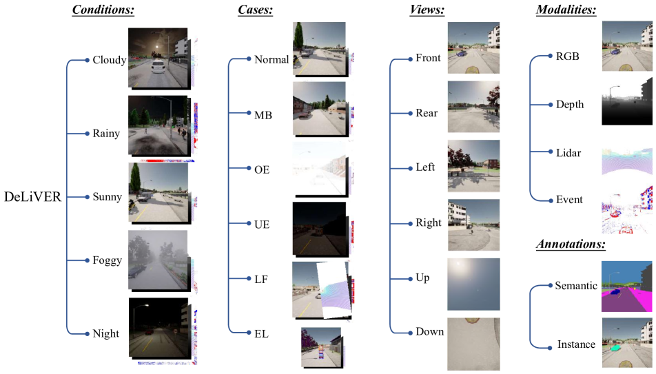
Figure 8: Data structure of the DeLiVER dataset. The columns from left to right are respective conditions, cases, multiple views, modalities and annotations. MB: Motion Blur; OE: Over-Exposure; UE: Under-Exposure; LJ: LiDAR-Jitter; and EL: Event Low-resolution.

A.2 Dataset structure

DeLiVER contains Depth, LiDAR, Event, and RGB modalities. As shown in Fig. 8, four adverse road scene conditions of rainy, sunny, foggy, and night are included in our dataset. There are five sensor failure cases including Motion Blur (MB), Over-Exposure (OE), Under-Exposure (UE), LiDAR-Jitter (LJ), and Event Low-resolution (EL) to verify that the performance of model is robust and stable in the presence of sensor failures. The sensors are mounted at different locations on the ego car to provide multiple views including front, rear, left, right, up, and down. Each sample is annotated with semantic and instance labels. In this work, we focus on the front-view semantic segmentation.

The $25$ semantic classes in DeLiVER dataset are: Building, Fence, Other, Pedestrian, Pole, RoadLine, Road, SideWalk, Vegetation, Cars, Wall, TrafficSign, Sky, Ground, Bridge, RailTrack, GroundRail, TrafficLight, Static, Dynamic, Water, Terrain, TwoWheeler, Bus, Truck.

A.3 Dataset statistics

Table 5: Data statistic of DeLiVER dataset. It includes four adverse conditions (cloudy, foggy, rainy, and night), and each condition has five failure cases (MB: Motion Blur; OE: Over-Exposure; UE: Under-Exposure; LJ: LiDAR-Jitter; and EL: Event Low-resolution).

Split	Cloudy	Foggy	Night	Rainny	Sunny	Total	Normal	MB	OE	UE	LJ	EL	Total
Train	794	795	797	799	798	3983	2585	600	200	199	199	200	3983
Val	398	400	410	398	399	2005	1298	299	100	99	100	109	2005
Test	379	379	379	380	380	1897	1198	300	100	100	99	100	1897
Front-view	1571	1574	1586	1577	1577	7885	5081	1199	400	398	398	409	7885
All six views	9426	9444	9516	9462	9462	47310	30486	7194	2400	2388	2388	2454	47310

We present statistics of the DeLiVER dataset in Table 5. We discuss data partitioning in two groups, one according to the conditions and the other according to the sensor failures. Note that, the two groups are mutually inclusive. The five cases from the second group are included in each of five conditions from the first group. For example, cases of MB, OE, UE, LJ, and EL are included in cloudy, foggy, night, rainy, and sunny conditions, but with different samples. To investigate the robustness under sensor failures, we collect $1199$, $400$, $398$, $398$, and $409$ frames on respective cases.

A.4 Dataset comparison

Table 6: Comparison between multimodal datasets. D:Day; S:Sunset; N:Night; *:random; Sem.:Semantic; Ins.:Instance.

Dataset	Type	Sensors				Sensor	RGB	Diversity			Classes	Labels
		Camera	Depth	Event	LiDAR	Failures	Failures	Weathers	Daytime	Views		Sem.	Ins.
WildDash [90]	Real	1	0	0	0	0	15	*	*	*	19	$\checkmark$	$\checkmark$
Waymo [65]	Real	5	0	0	5	0	0	2	DN	5	28	$\checkmark$	$\checkmark$
SELMA [68]	Synthetic	7	7	0	3	0	6	9	DSN	7	19	$\checkmark$	$\times$
SynWoodScape [59]	Synthetic	5	5	5	1	0	0	4	DS	5	25	$\checkmark$	$\checkmark$
SynPASS [94]	Synthetic	6	0	0	0	0	0	4	DN	1	22	$\checkmark$	$\times$
DeLiVER (ours)	Synthetic	6	6	6	1	5	3	4	DN	6	25	$\checkmark$	$\checkmark$

As shown in Table 6, we compare several datasets with adverse conditions and cases. All the datasets cover the whole daytime. The real-scene datasets, e.g., WildDash [90] and Waymo[65], capture data by using only one or a few sensors, which results a lack of data diversity. In contrast, our DeLiVER dataset has four different modalities, including RGB, Depth, Event and LiDAR, which enables the multimodal semantic segmentation task to involve up to $4$ modalities. Compared to previous synthetic datasets, e.g., SELMA [68], SynWoodScape [59], SynPASS [94], our DeLiVER additionally includes $5$ types of sensor failure. Each sample has semantic and instance annotations, so semantic, instance and panoptic segmentation tasks can be conducted on our DeLiVER dataset.

Appendix B Implementation Details

We conduct our experiments with PyTorch $1.9.0$. All models are trained on a node with 4 A100 GPUs. Below we describe the specific implementation details for six datasets.

Data representation. For depth images, we follow SA-Gate [11] and CMX [49] to preprocess the one-channel depth images to HHA-encoded representations [29], where HHA includes horizontal disparity, height above ground, and norm angle. The 3D LiDAR and Event data of DeLiVER dataset are transformed to the aforementioned frame format. Then, both LiDAR- and Event-based data are preprocessed as 2D range views [107] and 3-channel representations [95], respectively.

DeLiVER dataset. We train our models for $200$ epochs on the DeLiVER dataset. The batch size is $2$ on each of four GPUs. The resolution of all modalities is set as $1024{\times}1024$ for training and inference. In the Event Low-resolution cases, the Event-based images with the original size of $260{\times}260$ are upsampled to $1024{\times}1024$. During evaluation, we only apply the single-scale test strategy. The backbone of CMNeXt is based on MiT-B2 [80]. To verify the effectiveness of our method under convolutional networks, the CNN-based SegNeXt-Base [27] is selected as the backbone, when compared to the MiT-B2 one.

KITTI-360 dataset. As there are more than $49K$ training data on KITTI-360 dataset, the models are trained for $40$ epochs. The image resolution is set as $1408{\times}376$ and the batch size is $4$ on each of four GPUs. The backbone of CMNeXt is based on MiT-B2 [80].

NYU Depth V2 dataset. Following CMX [49], the number of training epochs is set as $500$ for a fair comparison. The resolution of RGB and Depth images is set as $640{\times}480$. The training batch size is $4$ on each of four GPUs. The backbone of CMNeXt is based on MiT-B4 [80]. We apply the multi-scale flip test strategy for a fair comparison.

MFNet dataset. We train our CMNeXt models with the MiT-B4 backbone for $500$ epochs on the MFNet dataset. The resolution of RGB and Thermal images is set as $640{\times}480$ and the batch size is $4$ on each of four GPUs. We apply the multi-scale flip test strategy for a fair comparison.

MCubeS dataset. To compare with MCubeSNet [45], we build CMNeXt with MiT-B2 and train the model for $500$ epochs. Following MCubeSNet [45], the image size is set as $512{\times}512$ during training and $1024{\times}1024$ during evaluation. The batch size is set as $4$ on each of four GPUs.

UrbanLF dataset. To perform comparison with the OCR-LF model [60], we build CMNeXt with MiT-B4. The image size on the real and synthetic sets is $640{\times}480$. The angular resolution of $81$ sub-aperture images of the UrbanLF dataset is $9{\times}9$. To conduct arbitrary-modal segmentation, the center-aperture image is selected as the primary modality, while the other apertures are as additional modalities. We sample respective $8$, $33$, and $80$ light field images as the supplementary modalities, i.e., LF$8$, LF$33$, and LF$80$ for short. The $8$ images are from the center horizontal direction, while the $33$ images are from the four directions of horizontal, vertical, $\frac{1}{4}\pi$, and $\frac{3}{4}\pi$, following UrbanLF [60].

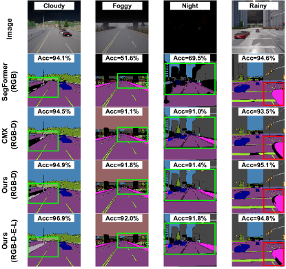
Figure 9: More visualization results on DeLiVER dataset. From left to right are the respective cloudy, foggy, night and rainy scene.

Appendix C More visualizations on DeLiVER

As shown in Fig. 9, in the four adverse weather conditions, RGB-D fusion-based methods greatly improve the performance, particularly for distant elements in foggy and nighttime scenes. Our RGB-D solution is more accurate than CMX (RGB-D), and the full quad-modal RGB-D-E-L CMNeXt model further enhances the segmentation. A failure case is shown on the right column (i.e., the rainy scene) of Fig. 9, in which the RGB-only model has a better segmentation on the sidewalk class. However, our quad-modal CMNeXt has a higher accuracy score with $94.8\%$.

Appendix D Acknowledgments

This work was supported in part by Helmholtz Association of German Research Centers, in part by the Federal Ministry of Labor and Social Affairs (BMAS) through the AccessibleMaps project under Grant 01KM151112, in part by the University of Excellence through the “KIT Future Fields” project, and in part by Hangzhou SurImage Technology Company Ltd. This work was partially performed on the HoreKa supercomputer funded by the Ministry of Science, Research and the Arts Baden-Württemberg and by the Federal Ministry of Education and Research.

References

- [1] Inigo Alonso and Ana C. Murillo. EV-SegNet: Semantic segmentation for event-based cameras. In CVPRW, 2019.
- [2] Roman Bachmann, David Mizrahi, Andrei Atanov, and Amir Zamir. MultiMAE: Multi-modal multi-task masked autoencoders. In ECCV, 2022.
- [3] Shubhankar Borse, Ying Wang, Yizhe Zhang, and Fatih Porikli. InverseForm: A loss function for structured boundary-aware segmentation. In CVPR, 2021.
- [4] Tim Broedermann, Christos Sakaridis, Dengxin Dai, and Luc Van Gool. HRFuser: A multi-resolution sensor fusion architecture for 2D object detection. arXiv preprint arXiv:2206.15157, 2022.
- [5] Jinming Cao, Hanchao Leng, Dani Lischinski, Daniel Cohen-Or, Changhe Tu, and Yangyan Li. ShapeConv: Shape-aware convolutional layer for indoor RGB-D semantic segmentation. In ICCV, 2021.
- [6] Jin Chen, Xijun Wang, Zichao Guo, Xiangyu Zhang, and Jian Sun. Dynamic region-aware convolution. In CVPR, 2021.
- [7] Liang-Chieh Chen, George Papandreou, Iasonas Kokkinos, Kevin Murphy, and Alan L. Yuille. DeepLab: Semantic image segmentation with deep convolutional nets, atrous convolution, and fully connected CRFs. TPAMI, 2018.
- [8] Liang-Chieh Chen, Yukun Zhu, George Papandreou, Florian Schroff, and Hartwig Adam. Encoder-decoder with atrous separable convolution for semantic image segmentation. In ECCV, 2018.
- [9] Lin-Zhuo Chen, Zheng Lin, Ziqin Wang, Yong-Liang Yang, and Ming-Ming Cheng. Spatial information guided convolution for real-time RGBD semantic segmentation. TIP, 2021.
- [10] Shoufa Chen, Enze Xie, Chongjian Ge, Ding Liang, and Ping Luo. CycleMLP: A MLP-like architecture for dense prediction. In ICLR, 2022.
- [11] Xiaokang Chen, Kwan-Yee Lin, Jingbo Wang, Wayne Wu, Chen Qian, Hongsheng Li, and Gang Zeng. Bi-directional cross-modality feature propagation with separation-and-aggregation gate for RGB-D semantic segmentation. In ECCV, 2020.
- [12] Bowen Cheng, Ishan Misra, Alexander G. Schwing, Alexander Kirillov, and Rohit Girdhar. Masked-attention mask transformer for universal image segmentation. In CVPR, 2022.
- [13] Bowen Cheng, Alex Schwing, and Alexander Kirillov. Per-pixel classification is not all you need for semantic segmentation. In NeurIPS, 2021.
- [14] Sungha Choi, Joanne T. Kim, and Jaegul Choo. Cars can’t fly up in the sky: Improving urban-scene segmentation via height-driven attention networks. In CVPR, 2020.
- [15] Fuqin Deng, Hua Feng, Mingjian Liang, Hongmin Wang, Yong Yang, Yuan Gao, Junfeng Chen, Junjie Hu, Xiyue Guo, and Tin Lun Lam. FEANet: Feature-enhanced attention network for RGB-thermal real-time semantic segmentation. In IROS, 2021.
- [16] Jia Deng, Wei Dong, Richard Socher, Li-Jia Li, Kai Li, and Li Fei-Fei. ImageNet: A large-scale hierarchical image database. In CVPR, 2009.
- [17] Henghui Ding, Xudong Jiang, Ai Qun Liu, Nadia Magnenat Thalmann, and Gang Wang. Boundary-aware feature propagation for scene segmentation. In ICCV, 2019.
- [18] Xiaoyi Dong, Jianmin Bao, Dongdong Chen, Weiming Zhang, Nenghai Yu, Lu Yuan, Dong Chen, and Baining Guo. CSWin transformer: A general vision transformer backbone with cross-shaped windows. In CVPR, 2022.
- [19] Alexey Dosovitskiy, German Ros, Felipe Codevilla, Antonio Lopez, and Vladlen Koltun. CARLA: An open urban driving simulator. In CoRL, 2017.
- [20] Oriel Frigo, Lucien Martin-Gaffé, and Catherine Wacongne. DooDLeNet: Double DeepLab enhanced feature fusion for thermal-color semantic segmentation. In CVPRW, 2022.
- [21] Jun Fu, Jing Liu, Haijie Tian, Yong Li, Yongjun Bao, Zhiwei Fang, and Hanqing Lu. Dual attention network for scene segmentation. In CVPR, 2019.
- [22] Guillermo Gallego, Tobi Delbrück, Garrick Orchard, Chiara Bartolozzi, Brian Taba, Andrea Censi, Stefan Leutenegger, Andrew J. Davison, Jörg Conradt, Kostas Daniilidis, and Davide Scaramuzza. Event-based vision: A survey. TPAMI, 2022.
- [23] Biao Gao, Yancheng Pan, Chengkun Li, Sibo Geng, and Huijing Zhao. Are we hungry for 3D LiDAR data for semantic segmentation? A survey of datasets and methods. T-ITS, 2022.
- [24] Daniel Gehrig, Michelle Rüegg, Mathias Gehrig, Javier Hidalgo-Carrió, and Davide Scaramuzza. Combining events and frames using recurrent asynchronous multimodal networks for monocular depth prediction. RA-L, 2021.
- [25] Rohit Girdhar, Mannat Singh, Nikhila Ravi, Laurens van der Maaten, Armand Joulin, and Ishan Misra. Omnivore: A single model for many visual modalities. In CVPR, 2022.
- [26] Jiaqi Gu, Hyoukjun Kwon, Dilin Wang, Wei Ye, Meng Li, Yu-Hsin Chen, Liangzhen Lai, Vikas Chandra, and David Z. Pan. Multi-scale high-resolution vision transformer for semantic segmentation. In CVPR, 2022.
- [27] Meng-Hao Guo, Cheng-Ze Lu, Qibin Hou, Zhengning Liu, Ming-Ming Cheng, and Shi-Min Hu. SegNeXt: Rethinking convolutional attention design for semantic segmentation. In NeurIPS, 2022.
- [28] Meng-Hao Guo, Cheng-Ze Lu, Zheng-Ning Liu, Ming-Ming Cheng, and Shi-Min Hu. Visual attention network. arXiv preprint arXiv:2202.09741, 2022.
- [29] Saurabh Gupta, Ross Girshick, Pablo Arbeláez, and Jitendra Malik. Learning rich features from RGB-D images for object detection and segmentation. In ECCV, 2014.
- [30] Qishen Ha, Kohei Watanabe, Takumi Karasawa, Yoshitaka Ushiku, and Tatsuya Harada. MFNet: Towards real-time semantic segmentation for autonomous vehicles with multi-spectral scenes. In IROS, 2017.
- [31] Caner Hazirbas, Lingni Ma, Csaba Domokos, and Daniel Cremers. FuseNet: Incorporating depth into semantic segmentation via fusion-based CNN architecture. In ACCV, 2016.
- [32] Qibin Hou, Zihang Jiang, Li Yuan, Ming-Ming Cheng, Shuicheng Yan, and Jiashi Feng. Vision permutator: A permutable MLP-like architecture for visual recognition. TPAMI, 2022.
- [33] Qibin Hou, Li Zhang, Ming-Ming Cheng, and Jiashi Feng. Strip pooling: Rethinking spatial pooling for scene parsing. In CVPR, 2020.
- [34] Jie Hu, Li Shen, and Gang Sun. Squeeze-and-excitation networks. In CVPR, 2018.
- [35] Xinxin Hu, Kailun Yang, Lei Fei, and Kaiwei Wang. ACNet: Attention based network to exploit complementary features for RGBD semantic segmentation. In ICIP, 2019.
- [36] Zilong Huang, Xinggang Wang, Lichao Huang, Chang Huang, Yunchao Wei, and Wenyu Liu. CCNet: Criss-cross attention for semantic segmentation. In ICCV, 2019.
- [37] Zhenchao Jin, Tao Gong, Dongdong Yu, Qi Chu, Jian Wang, Changhu Wang, and Jie Shao. Mining contextual information beyond image for semantic segmentation. In ICCV, 2021.
- [38] Hamid Reza Vaezi Joze, Amirreza Shaban, Michael L. Iuzzolino, and Kazuhito Koishida. MMTM: Multimodal transfer module for CNN fusion. In CVPR, 2020.
- [39] Agastya Kalra, Vage Taamazyan, Supreeth Krishna Rao, Kartik Venkataraman, Ramesh Raskar, and Achuta Kadambi. Deep polarization cues for transparent object segmentation. In CVPR, 2020.
- [40] Youngwan Lee, Jonghee Kim, Jeffrey Willette, and Sung Ju Hwang. MPViT: Multi-path vision transformer for dense prediction. In CVPR, 2022.
- [41] Gongyang Li, Yike Wang, Zhi Liu, Xinpeng Zhang, and Dan Zeng. RGB-T semantic segmentation with location, activation, and sharpening. TCSVT, 2022.
- [42] Xiangtai Li, Xia Li, Li Zhang, Guangliang Cheng, Jianping Shi, Zhouchen Lin, Shaohua Tan, and Yunhai Tong. Improving semantic segmentation via decoupled body and edge supervision. In ECCV, 2020.
- [43] Yingwei Li, Adams Wei Yu, Tianjian Meng, Benjamin Caine, Jiquan Ngiam, Daiyi Peng, Junyang Shen, Yifeng Lu, Denny Zhou, Quoc V. Le, Alan L. Yuille, and Mingxing Tan. DeepFusion: Lidar-camera deep fusion for multi-modal 3D object detection. In CVPR, 2022.
- [44] Dongze Lian, Zehao Yu, Xing Sun, and Shenghua Gao. AS-MLP: An axial shifted MLP architecture for vision. In ICLR, 2022.
- [45] Yupeng Liang, Ryosuke Wakaki, Shohei Nobuhara, and Ko Nishino. Multimodal material segmentation. In CVPR, 2022.
- [46] Yiyi Liao, Jun Xie, and Andreas Geiger. KITTI-360: A novel dataset and benchmarks for urban scene understanding in 2D and 3D. TPAMI, 2022.
- [47] Guosheng Lin, Anton Milan, Chunhua Shen, and Ian Reid. RefineNet: Multi-path refinement networks for high-resolution semantic segmentation. In CVPR, 2017.
- [48] Haisong Liu, Tao Lu, Yihui Xu, Jia Liu, Wenjie Li, and Lijun Chen. CamLiFlow: Bidirectional camera-LiDAR fusion for joint optical flow and scene flow estimation. In CVPR, 2022.
- [49] Huayao Liu, Jiaming Zhang, Kailun Yang, Xinxin Hu, and Rainer Stiefelhagen. CMX: Cross-modal fusion for RGB-X semantic segmentation with transformers. arXiv preprint arXiv:2203.04838, 2022.
- [50] Ze Liu, Yutong Lin, Yue Cao, Han Hu, Yixuan Wei, Zheng Zhang, Stephen Lin, and Baining Guo. Swin transformer: Hierarchical vision transformer using shifted windows. In ICCV, 2021.
- [51] Zhuang Liu, Hanzi Mao, Chao-Yuan Wu, Christoph Feichtenhofer, Trevor Darrell, and Saining Xie. A ConvNet for the 2020s. In CVPR, 2022.
- [52] Jonathan Long, Evan Shelhamer, and Trevor Darrell. Fully convolutional networks for semantic segmentation. In CVPR, 2015.
- [53] Ilya Loshchilov and Frank Hutter. Decoupled weight decay regularization. In ICLR, 2019.
- [54] Haiyang Mei, Bo Dong, Wen Dong, Jiaxi Yang, Seung-Hwan Baek, Felix Heide, Pieter Peers, Xiaopeng Wei, and Xin Yang. Glass segmentation using intensity and spectral polarization cues. In CVPR, 2022.
- [55] Aditya Prakash, Kashyap Chitta, and Andreas Geiger. Multi-modal fusion transformer for end-to-end autonomous driving. In CVPR, 2021.
- [56] Yongming Rao, Wenliang Zhao, Yansong Tang, Jie Zhou, Ser-Lam Lim, and Jiwen Lu. HorNet: Efficient high-order spatial interactions with recursive gated convolutions. In NeurIPS, 2022.
- [57] Hazem Rashed, Senthil Yogamani, Ahmad El-Sallab, Pavel Krizek, and Mohamed El-Helw. Optical flow augmented semantic segmentation networks for automated driving. In VISAPP, 2019.
- [58] Daniel Seichter, Mona Köhler, Benjamin Lewandowski, Tim Wengefeld, and Horst-Michael Gross. Efficient RGB-D semantic segmentation for indoor scene analysis. In ICRA, 2021.
- [59] Ahmed Rida Sekkat, Yohan Dupuis, Varun Ravi Kumar, Hazem Rashed, Senthil Yogamani, Pascal Vasseur, and Paul Honeine. SynWoodScape: Synthetic surround-view fisheye camera dataset for autonomous driving. RA-L, 2022.
- [60] Hao Sheng, Ruixuan Cong, Da Yang, Rongshan Chen, Sizhe Wang, and Zhenglong Cui. UrbanLF: A comprehensive light field dataset for semantic segmentation of urban scenes. TCSVT, 2022.
- [61] Shreyas S. Shivakumar, Neil Rodrigues, Alex Zhou, Ian D. Miller, Vijay Kumar, and Camillo J. Taylor. PST900: RGB-thermal calibration, dataset and segmentation network. In ICRA, 2020.
- [62] Nathan Silberman, Derek Hoiem, Pushmeet Kohli, and Rob Fergus. Indoor segmentation and support inference from RGBD images. In ECCV, 2012.
- [63] Hwanjun Song, Eunyoung Kim, Varun Jampan, Deqing Sun, Jae-Gil Lee, and Ming-Hsuan Yang. Exploiting scene depth for object detection with multimodal transformers. In BMVC, 2021.
- [64] Robin Strudel, Ricardo Garcia, Ivan Laptev, and Cordelia Schmid. Segmenter: Transformer for semantic segmentation. In ICCV, 2021.
- [65] Pei Sun, Henrik Kretzschmar, Xerxes Dotiwalla, Aurelien Chouard, Vijaysai Patnaik, Paul Tsui, James Guo, Yin Zhou, Yuning Chai, Benjamin Caine, Vijay Vasudevan, Wei Han, Jiquan Ngiam, Hang Zhao, Aleksei Timofeev, Scott M. Ettinger, Maxim Krivokon, Amy Gao, Aditya Joshi, Yu Zhang, Jonathon Shlens, Zhifeng Chen, and Dragomir Anguelov. Scalability in perception for autonomous driving: Waymo open dataset. In CVPR, 2020.
- [66] Yuxiang Sun, Weixun Zuo, Peng Yun, Hengli Wang, and Ming Liu. FuseSeg: Semantic segmentation of urban scenes based on RGB and thermal data fusion. T-ASE, 2021.
- [67] Towaki Takikawa, David Acuna, Varun Jampani, and Sanja Fidler. Gated-SCNN: Gated shape CNNs for semantic segmentation. In ICCV, 2019.
- [68] Paolo Testolina, Francesco Barbato, Umberto Michieli, Marco Giordani, Pietro Zanuttigh, and Michele Zorzi. SELMA: Semantic large-scale multimodal acquisitions in variable weather, daytime and viewpoints. arXiv preprint arXiv:2204.09788, 2022.
- [69] Abhinav Valada, Rohit Mohan, and Wolfram Burgard. Self-supervised model adaptation for multimodal semantic segmentation. IJCV, 2020.
- [70] Hao Wang, Weining Wang, and Jing Liu. Temporal memory attention for video semantic segmentation. In ICIP, 2021.
- [71] Wenhai Wang, Enze Xie, Xiang Li, Deng-Ping Fan, Kaitao Song, Ding Liang, Tong Lu, Ping Luo, and Ling Shao. Pyramid vision transformer: A versatile backbone for dense prediction without convolutions. In ICCV, 2021.
- [72] Yikai Wang, Xinghao Chen, Lele Cao, Wenbing Huang, Fuchun Sun, and Yunhe Wang. Multimodal token fusion for vision transformers. In CVPR, 2022.
- [73] Yikai Wang, Wenbing Huang, Fuchun Sun, Tingyang Xu, Yu Rong, and Junzhou Huang. Deep multimodal fusion by channel exchanging. In NeurIPS, 2020.
- [74] Yikai Wang, Fuchun Sun, Ming Lu, and Anbang Yao. Learning deep multimodal feature representation with asymmetric multi-layer fusion. In MM, 2020.
- [75] Wei Wu, Tao Chu, and Qiong Liu. Complementarity-aware cross-modal feature fusion network for RGB-T semantic segmentation. PR, 2022.
- [76] Yu-Huan Wu, Yun Liu, Xin Zhan, and Ming-Ming Cheng. P2T: Pyramid pooling transformer for scene understanding. TPAMI, 2022.
- [77] Zongwei Wu, Guillaume Allibert, Christophe Stolz, and Cédric Demonceaux. Depth-adapted CNN for RGB-D cameras. In ACCV, 2020.
- [78] Zhongwei Wu, Zhuyun Zhou, Guillaume Allibert, Christophe Stolz, Cédric Demonceaux, and Chao Ma. Transformer fusion for indoor RGB-D semantic segmentation. CVIU, 2022.
- [79] Kaite Xiang, Kailun Yang, and Kaiwei Wang. Polarization-driven semantic segmentation via efficient attention-bridged fusion. OE, 2021.
- [80] Enze Xie, Wenhai Wang, Zhiding Yu, Anima Anandkumar, Jose M. Alvarez, and Ping Luo. SegFormer: Simple and efficient design for semantic segmentation with transformers. In NeurIPS, 2021.
- [81] Zhaohu Xing, Lequan Yu, Liang Wan, Tong Han, and Lei Zhu. NestedFormer: Nested modality-aware transformer for brain tumor segmentation. In MICCAI, 2022.
- [82] Haofei Xu and Juyong Zhang. AANet: Adaptive aggregation network for efficient stereo matching. In CVPR, 2020.
- [83] Xu Yan, Jiantao Gao, Chaoda Zheng, Chao Zheng, Ruimao Zhang, Shenghui Cui, and Zhen Li. 2DPASS: 2D priors assisted semantic segmentation on LiDAR point clouds. In ECCV, 2022.
- [84] Xiaowen Ying and Mooi Choo Chuah. UCTNet: Uncertainty-aware cross-modal transformer network for indoor RGB-D semantic segmentation. In ECCV, 2022.
- [85] Changqian Yu, Jingbo Wang, Changxin Gao, Gang Yu, Chunhua Shen, and Nong Sang. Context prior for scene segmentation. In CVPR, 2020.
- [86] Weihao Yu, Mi Luo, Pan Zhou, Chenyang Si, Yichen Zhou, Xinchao Wang, Jiashi Feng, and Shuicheng Yan. MetaFormer is actually what you need for vision. In CVPR, 2022.
- [87] Yuhui Yuan, Xilin Chen, and Jingdong Wang. Object-contextual representations for semantic segmentation. In ECCV, 2020.
- [88] Yuhui Yuan, Rao Fu, Lang Huang, Weihong Lin, Chao Zhang, Xilin Chen, and Jingdong Wang. HRFormer: High-resolution vision transformer for dense predict. In NeurIPS, 2021.
- [89] Yuhui Yuan, Lang Huang, Jianyuan Guo, Chao Zhang, Xilin Chen, and Jingdong Wang. OCNet: Object context for semantic segmentation. IJCV, 2021.
- [90] Oliver Zendel, Katrin Honauer, Markus Murschitz, Daniel Steininger, and Gustavo Fernández Domínguez. WildDash - Creating hazard-aware benchmarks. In ECCV, 2018.
- [91] Bowen Zhang, Zhi Tian, Quan Tang, Xiangxiang Chu, Xiaolin Wei, Chunhua Shen, and Yifan Liu. SegViT: Semantic segmentation with plain vision transformers. In NeurIPS, 2022.
- [92] Guodong Zhang, Jing-Hao Xue, Pengwei Xie, Sifan Yang, and Guijin Wang. Non-local aggregation for RGB-D semantic segmentation. SPL, 2021.
- [93] Hang Zhang, Kristin Dana, Jianping Shi, Zhongyue Zhang, Xiaogang Wang, Ambrish Tyagi, and Amit Agrawal. Context encoding for semantic segmentation. In CVPR, 2018.
- [94] Jiaming Zhang, Kailun Yang, Chaoxiang Ma, Simon Reiß, Kunyu Peng, and Rainer Stiefelhagen. Bending reality: Distortion-aware transformers for adapting to panoramic semantic segmentation. In CVPR, 2022.
- [95] Jiaming Zhang, Kailun Yang, and Rainer Stiefelhagen. ISSAFE: Improving semantic segmentation in accidents by fusing event-based data. In IROS, 2021.
- [96] Qiang Zhang, Shenlu Zhao, Yongjiang Luo, Dingwen Zhang, Nianchang Huang, and Jungong Han. ABMDRNet: Adaptive-weighted bi-directional modality difference reduction network for RGB-T semantic segmentation. In CVPR, 2021.
- [97] Hengshuang Zhao, Jianping Shi, Xiaojuan Qi, Xiaogang Wang, and Jiaya Jia. Pyramid scene parsing network. In CVPR, 2017.
- [98] Sixiao Zheng, Jiachen Lu, Hengshuang Zhao, Xiatian Zhu, Zekun Luo, Yabiao Wang, Yanwei Fu, Jianfeng Feng, Tao Xiang, Philip H. S. Torr, and Li Zhang. Rethinking semantic segmentation from a sequence-to-sequence perspective with transformers. In CVPR, 2021.
- [99] Daquan Zhou, Zhiding Yu, Enze Xie, Chaowei Xiao, Animashree Anandkumar, Jiashi Feng, and Jose M. Alvarez. Understanding the robustness in vision transformers. In ICML, 2022.
- [100] Hao Zhou, Lu Qi, Zhaoliang Wan, Hai Huang, and Xu Yang. RGB-D co-attention network for semantic segmentation. In ACCV, 2020.
- [101] Heng Zhou, Chunna Tian, Zhenxi Zhang, Qizheng Huo, Yongqiang Xie, and Zhongbo Li. Multi-spectral fusion transformer network for RGB-thermal urban scene semantic segmentation. GRSL, 2022.
- [102] Jingkai Zhou, Varun Jampani, Zhixiong Pi, Qiong Liu, and Ming-Hsuan Yang. Decoupled dynamic filter networks. In CVPR, 2021.
- [103] Wujie Zhou, Jinfu Liu, Jingsheng Lei, Lu Yu, and Jenq-Neng Hwang. GMNet: Graded-feature multilabel-learning network for RGB-thermal urban scene semantic segmentation. TIP, 2021.
- [104] Wujie Zhou, Enquan Yang, Jingsheng Lei, Jian Wan, and Lu Yu. PGDENet: Progressive guided fusion and depth enhancement network for RGB-D indoor scene parsing. TMM, 2022.
- [105] Alex Zihao Zhu, Ziyun Wang, Kaung Khant, and Kostas Daniilidis. EventGAN: Leveraging large scale image datasets for event cameras. In ICCP, 2021.
- [106] Jiafan Zhuang, Zilei Wang, and Bingke Wang. Video semantic segmentation with distortion-aware feature correction. TCSVT, 2021.
- [107] Zhuangwei Zhuang, Rong Li, Kui Jia, Qicheng Wang, Yuanqing Li, and Mingkui Tan. Perception-aware multi-sensor fusion for 3D LiDAR semantic segmentation. In ICCV, 2021.