MixPHM: Redundancy-Aware Parameter-Efficient Tuning for
Low-Resource Visual Question Answering

Abstract

Recently, finetuning pretrained Vision-Language Models (VLMs) has been a prevailing paradigm for achieving state-of-the-art performance in Visual Question Answering (VQA). However, as VLMs scale, finetuning full model parameters for a given task in low-resource settings becomes computationally expensive, storage inefficient, and prone to overfitting. Current parameter-efficient tuning methods dramatically reduce the number of tunable parameters, but there still exists a significant performance gap with full finetuning. In this paper, we propose MixPHM, a redundancy-aware parameter-efficient tuning method that outperforms full finetuning in low-resource VQA. Specifically, MixPHM is a lightweight module implemented by multiple PHM-experts in a mixture-of-experts manner. To reduce parameter redundancy, MixPHM reparameterizes expert weights in a low-rank subspace and shares part of the weights inside and across experts. Moreover, based on a quantitative redundancy analysis for adapters, we propose Redundancy Regularization to reduce task-irrelevant redundancy while promoting task-relevant correlation in MixPHM representations. Experiments conducted on VQA v2, GQA, and OK-VQA demonstrate that MixPHM outperforms state-of-the-art parameter-efficient methods and is the only one consistently surpassing full finetuning.

1 Introduction

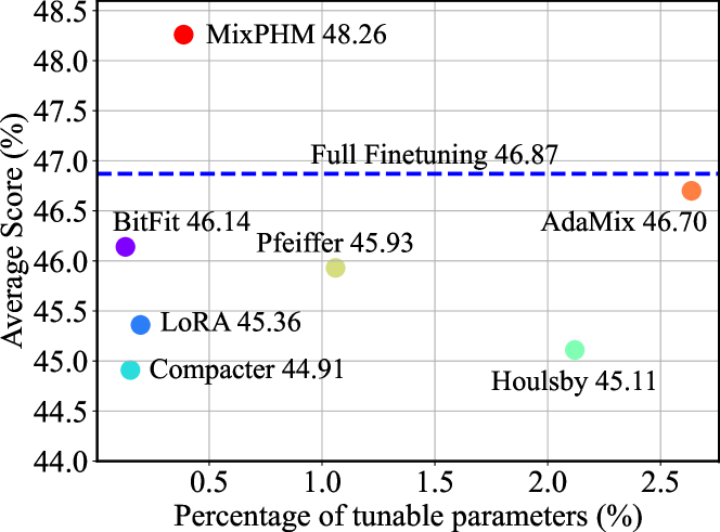
Figure 1: Comparison between parameter-efficient methods. In a low-resource setting (i.e., with 64 training samples), we show the average score across five seeds on VQA v2 (y-axis) and the percentage of tunable parameters w.r.t. pretrained VL-T5 (x-axis).

Adapting pretrained vision-language models (VLMs) [5, 31, 60, 25, 6, 30, 53] to the downstream VQA task [2] through finetuning has emerged as a dominant paradigm for achieving state-of-the-art performance. However, as the scale of VLMs continues to expand, finetuning an entire pretrained model that consists of millions or billions of parameters engenders a substantial increase in computational and storage costs, and exposes the risk of overfitting (poor performance) in low-resource learning. Parameter-efficient tuning methods, only updating newly-added lightweight modules (e.g., Houlsby [16], Pfeiffer [41], Compacter [24], and AdaMix [54]) or updating a tiny number of parameters in pretrained models (e.g., BitFit [59] and LoRA [17]), are thus proposed to handle these challenges.

However, as illustrated in Figure 1, the aforementioned parameter-efficient tuning methods substantially reduce the number of tunable parameters, but their performance still lags behind full finetuning. Among these methods, adapter-based approaches [16, 41, 24, 54] allow for more flexible parameter sharing [46] and are more storage-efficient by storing only a copy of these adapters instead of the entire pretrained model. In particular, AdaMix [54] employs adapters as experts within a mixture-of-experts (MoE) [45] architecture to enhance adapter capacity and achieves comparable performance to full finetuning. Nevertheless, this MoE mode leads to an increase in the number of tunable parameters due to parameter redundancy between adapters.

In this paper, we build upon adapter-based approaches to explore more parameter-efficient tuning methods that can outperform full finetuning on low-resource VQA. Specifically, when adapting pretrained VLMs to a given task, we focus on two key improvements: (i) Reducing parameter redundancy while maintaining adapter capacity. Striking a balance between parameter efficiency and model capacity is crucial since an excessive reduction of tunable parameters may lead to underfitting, limiting the ability of adapters to capture sufficient task-relevant information [24]. (ii) Reducing task-irrelevant redundancy while promoting task-relevant correlation in representations. In practice, adapters leverage residual connections to integrate task-specific information learned from a target dataset and prior knowledge already implied in pretrained VLMs. However, recent works [22, 35, 51] have highlighted that pretrained models inevitably contain redundant and irrelevant information for target tasks, resulting in statistically spurious correlations between representations and labels, thereby hindering performance and generalization [49, 52]. To enhance the effectiveness of adapters, our objective thus is to maximize the acquisition of task-relevant information while discarding task-irrelevant information from pretrained VLMs.

To this end, we propose MixPHM, a redundancy-aware parameter-efficient tuning method that can efficiently decrease tunable parameters and reduce task-irrelevant redundancy while promoting task-relevant correlation in representations. MixPHM is implemented with multiple PHM-experts in a MoE manner. To reduce (i) parameter redundancy, MixPHM first decomposes and reparameterizes expert weights into a low-rank subspace. Then, it further reduces tunable parameters and facilitates information transfer via global and local weight sharing. To achieve the improvement (ii), we first quantify the redundancy for adapters in representation spaces. The result reveals that adapter representations are redundant with pretrained VLM representations, but exhibit limited correlation to the final task-used representations. Motivated by this finding, we propose Redundancy Regularization, which is incorporated into MixPHM and serves to reduce task-irrelevant redundancy by decorrelating the similarity matrix between MixPHM representations and pretrained VLM representations. Simultaneously, it promotes task-relevant correlation by maximizing the mutual information between MixPHM representations and the final task-used representations.

We conduct experiments on VQA v2 [12], GQA [20], and OK-VQA [38], and demonstrate that the proposed MixPHM consistently outperforms full finetuning and state-of-the-art parameter-efficient tuning methods when adapting pretrained VLMs to low-resource VQA. In summary, our contributions are as follows: (1) We propose MixPHM, a redundancy-aware parameter-efficient tuning method for adapting pretrained VLMs to downstream tasks. (2) We propose Redundancy Regularization, a novel regularizer to reduce task-irrelevant redundancy while promoting task-relevant correlation in MixPHM representations. (3) Extensive experiments show MixPHM achieves a better trade-off between performance and parameter efficiency, leading to a significant performance gain over existing methods.

2 Related Work

Vision-Langauge Pretraining.  Vision-language pretraining [48, 9, 19, 63, 21, 25, 31, 6, 65] aims to learn task-agnostic multimodal representations for improving the performance of downstream tasks in a finetuning fashion. Recently, a line of research [5, 30, 31, 18, 53] has been devoted to leveraging encoder-decoder frameworks and generative modeling objectives to unify architectures and objectives between pretraining and finetuning. VLMs with an encoder-decoder architecture generalize better. In this paper, we explore how to better adapt them to low-resource VQA [2].

Parameter-Efficient Tuning.  Finetuning large-scale pretrained VLMs on given downstream datasets has become a mainstream paradigm for vision-language tasks. However, finetuning the full model consisting of millions of parameters is time-consuming and resource-intensive. Parameter-efficient tuning [59, 36, 44, 37, 13, 58, 62] vicariously tunes lightweight trainable parameters while keeping (most) pretrained parameters frozen, which has shown great success in NLP tasks. According to whether new trainable parameters are introduced, these methods can be roughly categorized into two groups: (1) tuning partial parameters of pretrained models, such as BitFit [59] and FISH Mask [47], (2) tuning additional parameters, such as prompt (prefix)-tuning [28, 32], adapter [16, 41], and low-rank methods [24, 17].

Motivated by the success in NLP, some works [33, 64, 46] have begun to introduce parameter-efficient methods to tune pretrained VLMs for vision-language tasks. Specifically, Lin et al. [33] investigate action-level prompts for vision-language navigation. VL-Adapter [46] extends adapters to transfer VLMs for various vision-language tasks. HyperPELT [64] is a unified parameter-efficient framework for vision-language tasks, incorporating adapter and prefix-tuning. In addition, Frozen [50] and PICa [57] use prompt-tuning techniques [28] to transfer the few-shot learning ability of large-scale pretrained language models to handle few-shot vision-language tasks. FewVLM [23] designs hand-crafted prompts to finetune pretrained VLMs for low-resource adaptation. In contrast, low-rank methods are more parameter-efficient but are rarely explored.

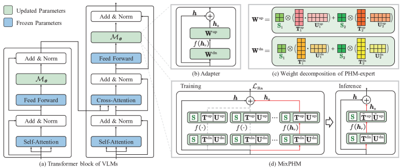
Figure 2: Illustration of MixPHM inserted into (a) one transformer block of VLMs. (b) The structure of standard adapter. (c) An example of the weight matrix decomposition in Eq. 13 for a PHM-expert (here $n=2$, $d=10$, $d_{r}=8$, $d_{k}=2$). (d) MixPHM architecture with $N_{e}=3$ PHM-experts. During training, MixPHM randomly activates one PHM-expert to learn robust representations and exploits the proposed redundancy regularization $\mathcal{L}_{\text{Ra}}$ to reduce task-irrelevant redundancy while promoting task-relevant correlation.

Mixture-of-Experts.  MoE [45] aims to scale up model capacities and keep computational efficiency with conditional computation. Most recent works [27, 8, 43, 29, 42, 7] investigate how to construct large-scale vision or language transformer models using MoE and well-designed routing mechanisms in the pretraining stage. Despite its success in pretraining, MoE has not been widely explored in parameter-efficient tuning. MPOE [11] and AdaMix [54] are two recent works that tune pretrained language models by MoE. Specifically, MPOE considers additional FFN layers as experts and decomposes weight matrices of experts with MPO. AdaMix treats the added adapters as experts and increases adapter capacity by a stochastic routing strategy.

3 Preliminary

Problem Definition.  We follow recent work [5, 55] to formulate VQA as a generative modeling task, i.e., generating free-form textual answers for a given question instead of selecting a specific one from the predefined set of answers. Formally, we denote a VQA dataset with $\mathcal{D}=\{(I,Q,y)\in\mathcal{I}\times\mathcal{Q}\times\mathcal{Y}\}$, where $I$ is an image, $Q$ is a question, and $y$ is an answer. Assuming that a given pretrained VLMs $\mathcal{M}_{\Theta}$ is parameterized by a tiny number of tunable parameters $\boldsymbol{\theta}$, the general problem of adapting pretrained VLMs for VQA is to tune $\mathcal{M}_{\boldsymbol{\theta}}$ in a parameter-efficient manner on $\mathcal{D}$.

Mixture-of-Experts.  A standard MoE [45] is implemented with a set of $N_{e}$ experts $\{E_{i}\}_{i=1}^{N_{e}}$ and a gating network $G$. Each expert is a sub-neural network with unique weights and can learn from a task-specific subset of inputs. The gate conditionally activates $N_{a}$ ($1\leq N_{a}\leq N_{e}$) experts. Formally, given an input representation $\boldsymbol{x}\in\mathbb{R}^{d}$, the $i$-th expert maps $\boldsymbol{x}$ into $d_{e}$-dimensional space, i.e., $E_{i}(\cdot):\boldsymbol{x}\rightarrow\mathbb{R}^{d_{e}}$, the gate generates a sparse ${N_{e}}$-dimensional vector, i.e., $G(\cdot):\boldsymbol{x}\rightarrow\mathbb{R}^{N_{e}}$. Then, the output $\boldsymbol{y}\in\mathbb{R}^{d_{e}}$ of the MoE can be formulated as

$$\boldsymbol{y}=\sum_{i=1}^{N_{e}}G(\boldsymbol{x})_{i}E_{i}(\boldsymbol{x}),$$ (1)

where, $G(\boldsymbol{x})_{i}$ denotes the probability of assigning $\boldsymbol{x}$ to the $i$-th expert, satisfying $\sum_{i=1}^{N_{e}}G(\boldsymbol{x})_{i}=1$.

Parameterized Hypercomplex Multiplication.  The PHM layer [61] aims to generalize hypercomplex multiplications to fully-connected layer by learning multiplication rules from data. Formally, for a fully-connected layer that transforms an input $\boldsymbol{x}\in\mathbb{R}^{d}$ to an output $\boldsymbol{y}\in\mathbb{R}^{d_{e}}$, i.e.,

$$\boldsymbol{y}=\mathbf{W}^{\mathrm{T}}\boldsymbol{x}+\boldsymbol{b},$$ (2)

where, $\mathbf{W}\in\mathbb{R}^{d\times d_{e}}$. In PHM, the weight matrix $\mathbf{W}$ is learned via the summation of $n$ Kronecker products between $\mathbf{S}_{j}\in\mathbb{R}^{n\times n}$ and $\mathbf{A}_{j}\in\mathbb{R}^{\frac{d}{n}\times\frac{d_{e}}{n}}$:

$$\mathbf{W}=\sum_{j=1}^{n}\mathbf{S}_{j}\otimes\mathbf{A}_{j},$$ (3)

where, the hyperparameter $n\in\mathbb{Z}_{>0}$ controls the number of the above summations, $d$ and $d_{e}$ are divisible by $n$, and $\otimes$ indicates the Kronecker product that generalizes the vector outer products to higher dimensions in real space. For example, the Kronecker product between $\mathbf{S}\in\mathbb{R}^{m\times k}$ and $\mathbf{A}\in\mathbb{R}^{p\times q}$ is a block matrix $\mathbf{S}\otimes\mathbf{A}\in\mathbb{R}^{mp\times kq}$, i.e.,

$$\mathbf{S}\otimes\mathbf{A}=\begin{bmatrix}s_{11}\mathbf{A}&\cdots&s_{1k}\mathbf{A}\\ \vdots&\ddots&\vdots\\ s_{m1}\mathbf{A}&\cdots&s_{mk}\mathbf{A}\end{bmatrix},$$ (4)

where, $s_{ij}$ denotes the element of matrix $\mathbf{S}$ at the $i$-th row and $j$-th column. As a result, replacing a fully-connected layer with PHM can reduce the trainable parameters by at most $1/n$ of the fully-connected layer.

4 Methodology

We propose MixPHM, a redundancy-aware parameter-efficient tuning method to adapt pretrained VLMs. This section first analyzes the redundancy in the adapter representation space toward low-resource VQA (Sec. 4.1). Then, we sequentially detail architecture (Sec. 4.2), redundancy regularization (Sec. 4.3), and inference (Sec. 4.4) of MixPHM.

4.1 Rethinking Redundancy in Adapter

As shown in Figure 2 (b), adapter [16] is essentially a lightweight module, usually implemented by a two-layer feed-forward network with a bottleneck, a nonlinear function, and a residual connection. When finetuning pretrained VLMs on downstream tasks, adapters are inserted between the transformer layers of VLMs, and only the parameters of the newly-added adapters are updated, while the original parameters in pretrained VLMs remain frozen. Formally, given an input representation $\boldsymbol{h}\in\mathbb{R}^{d}$, the down-projection layer $\mathbf{W}^{\text{dn}}\in\mathbb{R}^{d\times d_{r}}$ maps $\boldsymbol{h}$ to a lower-dimensional space specified by the bottleneck dimension $d_{r}$, i.e., $\boldsymbol{h}_{r}\in\mathbb{R}^{d_{r}}$. The up-projection layer $\mathbf{W}^{\text{up}}\in\mathbb{R}^{d_{r}\times d}$ maps $\boldsymbol{h}_{r}$ back to the input size, i.e., $\boldsymbol{h}_{a}\in\mathbb{R}^{d}$. Considering the residual and nonlinear function $f$, an adapter is defined as

$$\boldsymbol{h}_{a}=f(\boldsymbol{h}\mathbf{W}^{\text{dn}})\mathbf{W}^{\text{up}},$$ (5)

$$\boldsymbol{h}\leftarrow\boldsymbol{h}_{a}+\boldsymbol{h}.$$ (6)

Ideally, by incorporating task-specific information learned from a given downstream dataset ($\boldsymbol{h}_{a}$) and prior knowledge already encoded in pretrained VLMs ($\boldsymbol{h}$), adapters can quickly transfer pretrained VLMs to new tasks without over-parameterization or under-parameterization.

Redundancy Analysis for Adapter.  However, recent investigation has shown that some of the information captured by adapters is task-agnostic [14]. To get the facts, we leverage Representational Similarity Analysis (RSA) [26] to assess the redundancy in representation spaces. Specifically, we first tune the pretrained VL-T5 [5] with Pfeiffer [41] on 1k samples from VQA v2 training set [12]. Then, we randomly sample 1k samples from VQA v2 val set and extract token-level representations (i.e., $\boldsymbol{h}$ and $\boldsymbol{h}_{a}$) at each transformer layer as well as the final output representation $\tilde{\boldsymbol{h}}$ of transformer encoder/decoder. Finally, for each sample, we can obtain $N_{t}$ token-level representations at each layer, i.e., $\mathbf{H}=\{\boldsymbol{h}\}_{i=1}^{N_{t}}\in\mathbb{R}^{N_{t}\times d}$, $\mathbf{H}_{a}=\{\boldsymbol{h}_{a}\}_{i=1}^{N_{t}}\in\mathbb{R}^{N_{t}\times d}$ and $\tilde{\mathbf{H}}=\{\tilde{\boldsymbol{h}}\}_{i=1}^{N_{t}}\in\mathbb{R}^{N_{t}\times d}$. In each layer, we compute RSA similarity between $\boldsymbol{h}_{a}$ and $\boldsymbol{h}$ as well as $\boldsymbol{h}_{a}$ and $\tilde{\boldsymbol{h}}$ by

$$\text{RSA}(\boldsymbol{h}_{a},\boldsymbol{h})=f_{\rho}(f_{\text{U}}[\mathbf{H}_{a}\mathbf{H}_{a}^{\mathrm{T}}],f_{\text{U}}[\mathbf{H}\mathbf{H}^{\mathrm{T}}]),$$ (7)

$$\text{RSA}(\boldsymbol{h}_{a},\tilde{\boldsymbol{h}})=f_{\rho}(f_{\text{U}}[\mathbf{H}_{a}\mathbf{H}_{a}^{\mathrm{T}}],f_{\text{U}}[\tilde{\mathbf{H}}\tilde{\mathbf{H}}^{\mathrm{T}}]),$$ (8)

where, $f_{\text{U}}\left[\cdot\right]$ denotes an operation of taking the upper triangular elements from a matrix, $f_{\rho}$ is a function to compute the Pearson correlation coefficient. Figure 3 illustrates the average RSA similarity across 1k samples, which demonstrates that in transformer layers, the adapter representation $\boldsymbol{h}_{a}$ is redundant with the representation $\boldsymbol{h}$ of pretrained VLMs, but has limited correlation to the final output $\tilde{\boldsymbol{h}}$.

Intuitively, to transfer pretrained VLMs to downstream tasks efficiently, the representation $\boldsymbol{h}_{a}$ learned by adapter needs to contain as much information as possible from the task-relevant representation $\tilde{\boldsymbol{h}}$, while reducing task-irrelevant redundancy with the representation $\boldsymbol{h}$ of pretrained VLMs. However, Figure 3 exhibits a counterintuitive result. Therefore, in order to improve the effectiveness of adapters, it is crucial to encourage task-relevant correlation between $\boldsymbol{h}_{a}$ and $\tilde{\boldsymbol{h}}$ while reducing task-irrelevant redundancy between $\boldsymbol{h}_{a}$ and $\boldsymbol{h}$.

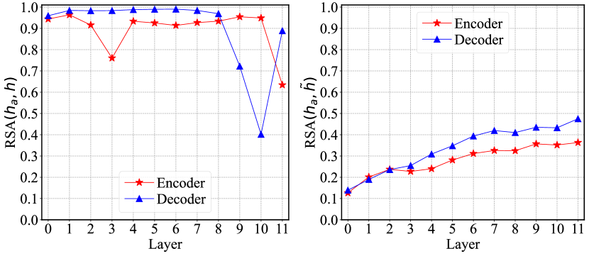
Figure 3: The average RSA similarity across 1k samples between $\boldsymbol{h}_{a}$ and $\boldsymbol{h}$ (left) as well as $\boldsymbol{h}_{a}$ and $\tilde{\boldsymbol{h}}$ (right) at each transformer layer. The higher the RSA, the more similar (redundant) the representation spaces are.

4.2 MixPHM Architecture

As illustrated in Figure 2, MixPHM is also a lightweight module inserted into each transformer block of VLMs. We utilize transformer-based encoder-decoder models as underlying pretrained VLMs, which consists of repeated $L$ encoder and $L$ decoder blocks. Specifically, for the $l$-th ($1\leq l\leq L$) block, we insert a MixPHM composed of a set of $N_{e}$ PHM-experts $\{E_{i}^{l}\}_{i=1}^{N_{e}}$ after the feed-forward layer to capture the knowledge and learn task-specific information. As with the adapter, each PHM-expert is implemented by a bottleneck network with down- and up-projection layers.

To reduce parameter redundancy in MixPHM, we first decompose and reparameterize the projection matrices of experts in MixPHM into low-dimensional subspace. Then, we further reduce the number of parameters and transfer information using a strategy of global and local expert weight sharing. Moreover, a stochastic routing [66, 54] is employed for expert selection to avoid gating networks from introducing additional trainable parameters.

Parameter-Efficient Tuning.  At each training (tuning) iteration, we randomly select one expert from the inserted $N_{e}$ PHM-experts in the $l$-th transformer block. Once the expert $E_{i}^{l}$ is selected, all inputs in a given batch are processed by the same expert. Formally, in the $l$-th block, for a token input representation $\boldsymbol{h}\in\mathbb{R}^{d}$, the randomly selected $i$-th expert encodes and updates $\boldsymbol{h}$ by

$$\boldsymbol{h}\leftarrow\leavevmode\nobreak\ f(\boldsymbol{h}\mathbf{W}_{i}^{\text{dn}})\mathbf{W}_{i}^{\text{up}}+\boldsymbol{h}.$$ (9)

In Eq. 9, the down-projection matrix $\mathbf{W}_{i}^{\text{dn}}\in\mathbb{R}^{d\times d_{r}}$ and up-projection matrix $\mathbf{W}_{i}^{\text{up}}\in\mathbb{R}^{d_{r}\times d}$ are firstly decomposed into low-dimensional matrices using PHM, i.e.,

$$\mathbf{W}_{i}^{\text{dn}}=\sum_{j=1}^{n}{\color[rgb]{0,.5,0}\mathbf{S}_{i,j}}\otimes\mathbf{A}_{i,j}^{\text{dn}}, \mathbf{W}_{i}^{\text{up}}=\sum_{j=1}^{n}{\color[rgb]{0,.5,0}\mathbf{S}_{i,j}}\otimes\mathbf{A}_{i,j}^{\text{up}},$$ (10)

where, ${\color[rgb]{0,.5,0}\mathbf{S}_{i,j}}\in\mathbb{R}^{n\times n}$, $\mathbf{A}_{i,j}^{\text{dn}}\in\mathbb{R}^{\frac{d}{n}\times\frac{d_{r}}{n}}$, $\mathbf{A}_{i,j}^{\text{up}}\in\mathbb{R}^{\frac{d_{r}}{n}\times\frac{d}{n}}$. To be more parameter-efficient, the matrix $\mathbf{A}_{i,j}^{\text{dn}}$ ($\mathbf{A}_{i,j}^{\text{up}}$) is further factorized into two low-rank matrices by

$$\mathbf{A}_{i,j}^{\text{dn}}=\mathbf{T}_{i,j}^{\text{dn}}(\mathbf{U}_{i,j}^{\text{dn}})^{\mathrm{T}}, \mathbf{A}_{i,j}^{\text{up}}=\mathbf{T}_{i,j}^{\text{up}}(\mathbf{U}_{i,j}^{\text{up}})^{\mathrm{T}},$$ (11)

where, $\mathbf{T}_{i,j}^{\text{dn}}\in\mathbb{R}^{\frac{d}{n}\times d_{k}}$, $\mathbf{U}_{i,j}^{\text{dn}}\in\mathbb{R}^{\frac{d_{r}}{n}\times d_{k}}$, $\mathbf{T}_{i,j}^{\text{up}}\in\mathbb{R}^{\frac{d_{r}}{n}\times d_{k}}$, $\mathbf{U}_{i,j}^{\text{up}}\in\mathbb{R}^{\frac{d}{n}\times d_{k}}$, and $d_{r}$ is the rank of these matrices. Finally, we learn the weight matrices of the $i$-th PHM-expert by

$$\mathbf{W}_{i}^{\text{dn}}=\sum_{j=1}^{n}{\color[rgb]{0,.5,0}\mathbf{S}_{i,j}}\otimes(\mathbf{T}_{i,j}^{\text{dn}}(\mathbf{U}_{i,j}^{\text{dn}})^{\mathrm{T}}),$$ (12)

$$\mathbf{W}_{i}^{\text{up}}=\sum_{j=1}^{n}{\color[rgb]{0,.5,0}\mathbf{S}_{i,j}}\otimes(\mathbf{T}_{i,j}^{\text{up}}(\mathbf{U}_{i,j}^{\text{up}})^{\mathrm{T}}).$$ (13)

Information Sharing across PHM-Experts.  When tuning pretrained VLMs with MixPHM on a downstream dataset, the set of $n$ matrices $\{{\color[rgb]{0,.5,0}\mathbf{S}_{i,j}}\in\mathbb{R}^{n\times n}\}_{j=1}^{n}$ of the $i$-th PHM-expert are globally shared among all PHM-experts across transformer blocks to capture general information for the target task. In other words, the ${\color[rgb]{0,.5,0}\mathbf{S}}=\{{\color[rgb]{0,.5,0}\mathbf{S}}_{j}\}_{j=1}^{n}\in\mathbb{R}^{n\times n\times n}$ of one expert is shared between all added MixPHMs. On the contrary, $\{\mathbf{A}_{i,j}^{\text{dn}}\}_{j=1}^{n}$ and $\{\mathbf{A}_{i,j}^{\text{up}}\}_{j=1}^{n}$ are expert-specific weight matrices which are unique to each PHM-expert. To better transfer information between PHM-experts of MixPHM and further reduce parameter redundancy, we locally share $\{\mathbf{A}_{i,j}^{\text{dn}}\}_{j=1}^{n}$ among PHM-experts in each MixPHM.

At this point, the total number of trainable parameters inserted into pretrained VLMs using MixPHM is reduced from the original $4LN_{e}(dd_{r})$ to $2Ld_{k}(d+d_{r})(N_{e}+1)+n^{3}$.

4.3 Redundancy Regularization

Motivated by the insight discussed in Sec. 4.1, we propose redundancy regularization. Specifically, for the MixPHM in the $l$-th transformer block, we ensemble its token-level output representation $\{\boldsymbol{h}_{a}\}_{i=1}^{N}$ and its residual $\{\boldsymbol{h}\}_{i=1}^{N}$ of a batch to $\mathbf{Z}_{a}\in\mathbb{R}^{N\times d}$ and $\mathbf{Z}\in\mathbb{R}^{N\times d}$, $N=N_{b}N_{t}$ ($N_{b}$ indicates batch size). For the transformer encoder/decoder, we average the final output representation $\{\tilde{\boldsymbol{h}}\}_{i=1}^{N}$ of a batch along the token dimension and obtain a global task-relevant representation $\{\bar{\boldsymbol{h}}\}_{i=1}^{N_{b}}$. Then, the redundancy regularization can be expressed by

$$\mathcal{L}_{\text{Ra}}\triangleq\sum_{i}^{N}\sum_{j\neq i}^{N}\frac{\mathbf{Z}_{a}\mathbf{Z}^{\mathrm{T}}}{\left\|\mathbf{Z}_{a}\right\|_{2}\left\|\mathbf{Z}\right\|_{2}}-\sum_{i}^{N_{b}}\sum_{j}^{N_{t}}\hat{\mathcal{I}}({\boldsymbol{h}_{a}}_{i,j};\bar{\boldsymbol{h}}_{i}),$$ (14)

where, $\left\|\cdot\right\|_{2}$ denotes the $L_{2}$ norm, ${\boldsymbol{h}_{a}}_{i,j}$ is the output representation of the $j$-th token of the $i$-th sample in a batch, and $\hat{\mathcal{I}}(\cdot;\cdot)$ means an estimation of mutual information (MI), which is used to maximize the correction between two representations and computed by the JSD MI estimator [15]. In redundancy regularization $\mathcal{L}_{\text{Ra}}$, the first term is a redundancy reduction term, which encourages $\boldsymbol{h}_{a}$ to discard task-irrelevant information from pretrained VLMs by encouraging the off-diagonal elements of the cosine similarity matrix between $\boldsymbol{h}_{a}$ and $\boldsymbol{h}$ to zero. The second term aims to advocate $\boldsymbol{h}_{a}$ contain more task-relevant information from downstream datasets by maximizing the MI between $\boldsymbol{h}_{a}$ and $\bar{\boldsymbol{h}}$.

Formulating VQA as a generative task, the training objective is to minimize the negative log-likelihood of answer $y$ tokens given input image $I$ and question $Q$. Therefore, the total training loss in parameter-efficient tuning is

$$\mathcal{L}=-\sum_{j=1}^{|y|}\log P_{\boldsymbol{\theta}}(y_{j}|y_{<j};I,Q)+\alpha\mathcal{L}_{\text{Ra}},$$ (15)

where, $\alpha$ is a factor to balance redundancy regularization.

4.4 Inference

In contrast to the stochastic routing utilized during training, we adopt a weight aggregation strategy [56] to obtain a final PHM-expert for each MixPHM during inference. Specifically, one MixPHM has $N_{e}$ PHM-experts. When learning weights in a low-rank subspace, each expert has $2n$ expert-specific matrices $\{\mathbf{T}_{j}^{\text{up}},\mathbf{U}_{j}^{\text{up}}\}_{j=1}^{n}$, and the $N_{e}$ experts have the same $2n$ locally-shared matrices $\{\mathbf{T}_{j}^{\text{dn}},\mathbf{U}_{j}^{\text{dn}}\}_{j=1}^{n}$ as well as $n$ globally-shared matrices $\{{\color[rgb]{0,.5,0}\mathbf{S}_{j}}\}_{j=1}^{n}$. To obtain weights of the final PHM-expert, we first merge the weights of up-projection matrices by averaging the corresponding $N_{e}$ weight matrices. Mathematically, the $j$-th up-projection matrices can be computed with

$$\widetilde{\mathbf{T}}_{j}^{\text{up}}=\frac{1}{N_{e}}\sum_{i=1}^{N_{e}}\mathbf{T}_{ji}^{\text{up}},\quad\widetilde{\mathbf{U}}_{j}^{\text{up}}=\frac{1}{N_{e}}\sum_{i=1}^{N_{e}}\mathbf{U}_{ji}^{\text{up}}.$$ (16)

Due to the global and local weight sharing, we need not perform weight aggregation on ${\color[rgb]{0,.5,0}\mathbf{S}}$ and $\{\mathbf{T}_{j}^{\text{dn}},\mathbf{U}_{j}^{\text{dn}}\}_{j=1}^{n}$. Finally, we employ the merged expert to compute the output representations of MixPHM at each transformer block.

Dataset	Method	#Param		#Sample
		(M)	(%)	$N_{\mathcal{D}}$=16	$N_{\mathcal{D}}$=32	$N_{\mathcal{D}}$=64	$N_{\mathcal{D}}$=100	$N_{\mathcal{D}}$=500	$N_{\mathcal{D}}$=1,000
	Finetuning	224.54	100%	41.82$\leavevmode\nobreak\ {}_{\pm{1.58}}$	43.09$\leavevmode\nobreak\ {}_{\pm{3.10}}$	46.87$\leavevmode\nobreak\ {}_{\pm{0.57}}$	48.12$\leavevmode\nobreak\ {}_{\pm{0.87}}$	53.46$\leavevmode\nobreak\ {}_{\pm{0.41}}$	55.56$\leavevmode\nobreak\ {}_{\pm{0.13}}$
	BitFit [59]	0.29	0.13%	40.61$\leavevmode\nobreak\ {}_{\pm{4.15}}$	43.86$\leavevmode\nobreak\ {}_{\pm{2.19}}$	46.14$\leavevmode\nobreak\ {}_{\pm{1.00}}$	47.53$\leavevmode\nobreak\ {}_{\pm{0.67}}$	51.91$\leavevmode\nobreak\ {}_{\pm{0.40}}$	53.18$\leavevmode\nobreak\ {}_{\pm{0.58}}$
	LoRA [17]	0.44	0.20%	41.60$\leavevmode\nobreak\ {}_{\pm{2.27}}$	42.62$\leavevmode\nobreak\ {}_{\pm{2.41}}$	45.36$\leavevmode\nobreak\ {}_{\pm{1.66}}$	47.57$\leavevmode\nobreak\ {}_{\pm{0.91}}$	51.93$\leavevmode\nobreak\ {}_{\pm{0.38}}$	54.15$\leavevmode\nobreak\ {}_{\pm{0.45}}$
	Compacter [24]	0.34	0.15%	39.28$\leavevmode\nobreak\ {}_{\pm{1.87}}$	42.47$\leavevmode\nobreak\ {}_{\pm{2.76}}$	44.91$\leavevmode\nobreak\ {}_{\pm{1.27}}$	46.28$\leavevmode\nobreak\ {}_{\pm{1.37}}$	51.21$\leavevmode\nobreak\ {}_{\pm{0.90}}$	53.39$\leavevmode\nobreak\ {}_{\pm{0.54}}$
	Houlsby [16]	4.76	2.12%	41.71$\leavevmode\nobreak\ {}_{\pm{2.16}}$	44.01$\leavevmode\nobreak\ {}_{\pm{2.09}}$	45.11$\leavevmode\nobreak\ {}_{\pm{1.40}}$	47.71$\leavevmode\nobreak\ {}_{\pm{0.78}}$	52.27$\leavevmode\nobreak\ {}_{\pm{1.05}}$	54.31$\leavevmode\nobreak\ {}_{\pm{0.34}}$
	Pfeiffer [41]	2.38	1.06%	41.48$\leavevmode\nobreak\ {}_{\pm{1.86}}$	44.18$\leavevmode\nobreak\ {}_{\pm{2.13}}$	45.93$\leavevmode\nobreak\ {}_{\pm{1.11}}$	47.42$\leavevmode\nobreak\ {}_{\pm{1.15}}$	52.35$\leavevmode\nobreak\ {}_{\pm{0.52}}$	53.98$\leavevmode\nobreak\ {}_{\pm{0.38}}$
	AdaMix [54]	5.92	2.64%	40.59$\leavevmode\nobreak\ {}_{\pm{2.05}}$	43.42$\leavevmode\nobreak\ {}_{\pm{2.08}}$	46.70$\leavevmode\nobreak\ {}_{\pm{1.32}}$	47.34$\leavevmode\nobreak\ {}_{\pm{0.91}}$	51.72$\leavevmode\nobreak\ {}_{\pm{1.05}}$	54.12$\leavevmode\nobreak\ {}_{\pm{0.63}}$
VQA v2 [12]	MixPHM	0.87	0.39%	43.13$\leavevmode\nobreak\ {}_{\pm{1.78}}$	45.97$\leavevmode\nobreak\ {}_{\pm{2.01}}$	48.26$\leavevmode\nobreak\ {}_{\pm{0.56}}$	49.91$\leavevmode\nobreak\ {}_{\pm{0.76}}$	54.30$\leavevmode\nobreak\ {}_{\pm{0.33}}$	56.11$\leavevmode\nobreak\ {}_{\pm{0.40}}$
	Finetuning	224.54	100%	28.24$\leavevmode\nobreak\ {}_{\pm{2.08}}$	30.80$\leavevmode\nobreak\ {}_{\pm{2.49}}$	34.22$\leavevmode\nobreak\ {}_{\pm{0.59}}$	36.15$\leavevmode\nobreak\ {}_{\pm{0.99}}$	41.49$\leavevmode\nobreak\ {}_{\pm{0.54}}$	43.04$\leavevmode\nobreak\ {}_{\pm{0.57}}$
	BitFit [59]	0.29	0.13%	26.13$\leavevmode\nobreak\ {}_{\pm{2.83}}$	29.00$\leavevmode\nobreak\ {}_{\pm{4.81}}$	34.25$\leavevmode\nobreak\ {}_{\pm{1.16}}$	35.91$\leavevmode\nobreak\ {}_{\pm{1.22}}$	40.08$\leavevmode\nobreak\ {}_{\pm{0.42}}$	41.84$\leavevmode\nobreak\ {}_{\pm{0.15}}$
	LoRA [17]	0.44	0.20%	26.89$\leavevmode\nobreak\ {}_{\pm{2.74}}$	30.40$\leavevmode\nobreak\ {}_{\pm{2.27}}$	34.40$\leavevmode\nobreak\ {}_{\pm{0.99}}$	36.14$\leavevmode\nobreak\ {}_{\pm{1.10}}$	40.20$\leavevmode\nobreak\ {}_{\pm{1.02}}$	42.06$\leavevmode\nobreak\ {}_{\pm{1.12}}$
	Compacter [24]	0.34	0.15%	23.70$\leavevmode\nobreak\ {}_{\pm{2.10}}$	27.18$\leavevmode\nobreak\ {}_{\pm{2.61}}$	32.70$\leavevmode\nobreak\ {}_{\pm{1.30}}$	35.28$\leavevmode\nobreak\ {}_{\pm{1.45}}$	38.68$\leavevmode\nobreak\ {}_{\pm{0.50}}$	41.17$\leavevmode\nobreak\ {}_{\pm{0.95}}$
	Houlsby [16]	4.76	2.12%	25.13$\leavevmode\nobreak\ {}_{\pm{2.32}}$	28.34$\leavevmode\nobreak\ {}_{\pm{1.17}}$	33.23$\leavevmode\nobreak\ {}_{\pm{0.94}}$	35.88$\leavevmode\nobreak\ {}_{\pm{1.79}}$	40.85$\leavevmode\nobreak\ {}_{\pm{0.48}}$	41.90$\leavevmode\nobreak\ {}_{\pm{0.72}}$
	Pfeiffer [41]	2.38	1.06%	25.08$\leavevmode\nobreak\ {}_{\pm{1.81}}$	29.18$\leavevmode\nobreak\ {}_{\pm{1.32}}$	32.97$\leavevmode\nobreak\ {}_{\pm{0.84}}$	35.08$\leavevmode\nobreak\ {}_{\pm{1.01}}$	40.30$\leavevmode\nobreak\ {}_{\pm{0.40}}$	41.39$\leavevmode\nobreak\ {}_{\pm{0.27}}$
	AdaMix [54]	5.92	2.64%	24.62$\leavevmode\nobreak\ {}_{\pm{2.34}}$	28.01$\leavevmode\nobreak\ {}_{\pm{1.33}}$	32.74$\leavevmode\nobreak\ {}_{\pm{0.96}}$	35.64$\leavevmode\nobreak\ {}_{\pm{0.94}}$	40.14$\leavevmode\nobreak\ {}_{\pm{0.42}}$	41.97$\leavevmode\nobreak\ {}_{\pm{0.86}}$
GQA [20]	MixPHM	0.87	0.39%	28.33$\leavevmode\nobreak\ {}_{\pm{2.63}}$	32.40$\leavevmode\nobreak\ {}_{\pm{2.52}}$	36.75$\leavevmode\nobreak\ {}_{\pm{0.55}}$	37.40$\leavevmode\nobreak\ {}_{\pm{0.87}}$	41.92$\leavevmode\nobreak\ {}_{\pm{0.55}}$	43.81$\leavevmode\nobreak\ {}_{\pm{0.50}}$
	Finetuning	224.54	100%	11.66$\leavevmode\nobreak\ {}_{\pm{2.08}}$	14.20$\leavevmode\nobreak\ {}_{\pm{0.78}}$	16.65$\leavevmode\nobreak\ {}_{\pm{1.02}}$	18.28$\leavevmode\nobreak\ {}_{\pm{0.67}}$	24.07$\leavevmode\nobreak\ {}_{\pm{0.40}}$	26.66$\leavevmode\nobreak\ {}_{\pm{0.72}}$
	BitFit [59]	0.29	0.13%	11.29$\leavevmode\nobreak\ {}_{\pm{1.79}}$	13.66$\leavevmode\nobreak\ {}_{\pm{1.49}}$	15.29$\leavevmode\nobreak\ {}_{\pm{0.57}}$	16.51$\leavevmode\nobreak\ {}_{\pm{0.53}}$	22.54$\leavevmode\nobreak\ {}_{\pm{0.57}}$	24.80$\leavevmode\nobreak\ {}_{\pm{0.63}}$
	LoRA [17]	0.44	0.20%	10.26$\leavevmode\nobreak\ {}_{\pm{1.53}}$	12.46$\leavevmode\nobreak\ {}_{\pm{1.82}}$	15.95$\leavevmode\nobreak\ {}_{\pm{0.38}}$	17.03$\leavevmode\nobreak\ {}_{\pm{0.82}}$	23.02$\leavevmode\nobreak\ {}_{\pm{0.41}}$	25.26$\leavevmode\nobreak\ {}_{\pm{0.53}}$
	Compacter [24]	0.34	0.15%	9.64$\leavevmode\nobreak\ {}_{\pm{2.73}}$	11.04$\leavevmode\nobreak\ {}_{\pm{1.39}}$	13.57$\leavevmode\nobreak\ {}_{\pm{1.07}}$	15.92$\leavevmode\nobreak\ {}_{\pm{1.18}}$	22.20$\leavevmode\nobreak\ {}_{\pm{0.89}}$	24.52$\leavevmode\nobreak\ {}_{\pm{0.59}}$
	Houlsby [16]	4.76	2.12%	9.79$\leavevmode\nobreak\ {}_{\pm{1.71}}$	12.25$\leavevmode\nobreak\ {}_{\pm{2.13}}$	15.04$\leavevmode\nobreak\ {}_{\pm{1.25}}$	16.58$\leavevmode\nobreak\ {}_{\pm{0.65}}$	22.67$\leavevmode\nobreak\ {}_{\pm{0.77}}$	25.04$\leavevmode\nobreak\ {}_{\pm{0.44}}$
	Pfeiffer [41]	2.38	1.06%	9.06$\leavevmode\nobreak\ {}_{\pm{0.53}}$	11.39$\leavevmode\nobreak\ {}_{\pm{0.79}}$	14.23$\leavevmode\nobreak\ {}_{\pm{1.54}}$	16.34$\leavevmode\nobreak\ {}_{\pm{0.79}}$	22.90$\leavevmode\nobreak\ {}_{\pm{1.03}}$	26.70$\leavevmode\nobreak\ {}_{\pm{0.71}}$
	AdaMix [54]	5.92	2.64%	8.39$\leavevmode\nobreak\ {}_{\pm{1.20}}$	11.55$\leavevmode\nobreak\ {}_{\pm{1.37}}$	13.66$\leavevmode\nobreak\ {}_{\pm{2.29}}$	16.27$\leavevmode\nobreak\ {}_{\pm{0.92}}$	23.20$\leavevmode\nobreak\ {}_{\pm{0.78}}$	26.34$\leavevmode\nobreak\ {}_{\pm{0.88}}$
OK-VQA [38]	MixPHM	0.87	0.39%	13.87$\leavevmode\nobreak\ {}_{\pm{2.39}}$	16.03$\leavevmode\nobreak\ {}_{\pm{1.23}}$	18.58$\leavevmode\nobreak\ {}_{\pm{1.42}}$	20.16$\leavevmode\nobreak\ {}_{\pm{0.97}}$	26.08$\leavevmode\nobreak\ {}_{\pm{0.88}}$	28.53$\leavevmode\nobreak\ {}_{\pm{0.85}}$

Table 1: Experimental results with pretrained VL-T5. The average VQA-Score with standard deviation across 5 seeds are evaluated on VQA v2 validation set, GQA test-dev, and OK-VQA test set. The best and second best parameter-efficient tuning methods are highlighted. The number of tuned parameters and the percentage of tuned parameters relative to VL-T5 (i.e., 224.54M) are reported.

5 Experiment

5.1 Experimental Setting

Datasets and Metrics.  We conduct experiments on three datasets, VQA v2 [12], GQA [20], and OK-VQA [38]. To simulate the low-resource setting for VQA, we follow the work [4] and consider the training data size $N_{\mathcal{D}}$ for low-resource VQA to be smaller than 1,000. For more practical low-resource learning, we follow true few-shot learning [40, 10] and utilize the development set $\mathcal{D}_{\text{dev}}$, which has the same size with the training set $\mathcal{D}_{\text{train}}$ (i.e., $|\mathcal{D}_{\text{dev}}|=$ $|\mathcal{D}_{\text{train}}|=$ $N_{\mathcal{D}}$), instead of using large-scale validation set, for best model selection and hyperparameter tuning. Specifically, we conduct experiments on $N_{\mathcal{D}}\in\{16,32,64,100,500,1000\}$. To construct the $\mathcal{D}_{\text{train}}$ and $\mathcal{D}_{\text{dev}}$ of VQA v2, we randomly sample $2N_{\mathcal{D}}$ samples from its training set and divide them equally into the $\mathcal{D}_{\text{train}}$ and $\mathcal{D}_{\text{dev}}$. Analogously, we construct $\mathcal{D}_{\text{train}}$ and $\mathcal{D}_{\text{dev}}$ for GQA and OK-VQA. VQA-Score [2] is the accuracy metric of the low-resource VQA task.

Baselines.  We compare our method with several state-of-the-art parameter-efficient tuning methods and finetuning. For a fair comparison, we perform hyperparameter search on their key hyperparameters (KHP) and report their best performance. Specifically,

• BitFit [59] only tunes the bias weights of pretrained models while keeping the rest parameters frozen.

• LoRA [17] tunes additional low-rank matrices, which are used to approximate the query and value weights in each transformer self-attention and cross-attention layer. KHP is the matrix rank ($r$).

• Compacter [24] adds adapters after each feed-forward layer of transformer blocks and reparameterizes adapter weights with low-rank PHM layers [61]. KHP are the number of summations of Kronecker product ($n$), the bottleneck dimension ($d_{r}$), and $r$.

• Houlsby [16] adds adapters after self-attention and feed-forward layers in each transformer block. KHP is $d_{r}$.

• Pfeiffer [41] is to determine the location of adapter based on pilot experiments. In this work, we place it after each transformer feed-forward layer. KHP is $d_{r}$.

• AdaMix [54] adds multiple adapters after each transformer feed-forward layer in a MoE manner. KHP are the number of adapters ($N_{e}$), and $d_{r}$.

Method	Model Size	#Param (%)	VQAv2	GQA	OK-VQA
Frozen [50]	7B	-	38.2	12.6	-
PICa-Base [57]	175B	-	54.3	43.3	-
PICa-Full [57]	175B	-	56.1	48.0	-
FewVLM [23]	225M	100%	48.2	32.2	15.0
MixPHM†	226M	0.39%	49.3	33.4	19.2

Table 2: Comparison with few-shot learner ($N_{\mathcal{D}}$=64). FewVLM is a prompt-based full finetuning method. MixPHM^† means using MixPHM to tune FewVLM in a parameter-efficient manner.

Implementation Details.  We use four pretrained VLMs, i.e., VL-T5 [5], X-VLM [60], BLIP [30], and OFA${}_{\text{Base}}$ [53], as underlying encoder-decoder transformers, which formulate VQA as a generation task in finetuning and thus do not introduce additional parameters from VQA heads. Since the original pretraining datasets employed by VL-T5 contain samples of the above VQA datasets, we instead load the weights released by Jin et al. [23], which is re-trained without the overlapped samples. All results are reported across five seeds $\{13,21,42,87,100\}$. More details and hyperparameter setups are provided in Appendix D.

Method	VQA v2	GQA	OK-VQA
Finetuning	46.87$\leavevmode\nobreak\ {}_{\pm{0.57}}$	34.22$\leavevmode\nobreak\ {}_{\pm{0.59}}$	16.65$\leavevmode\nobreak\ {}_{\pm{1.02}}$
MixPHM∗	47.30$\leavevmode\nobreak\ {}_{\pm{0.67}}$	34.66$\leavevmode\nobreak\ {}_{\pm{0.78}}$	18.05$\leavevmode\nobreak\ {}_{\pm{1.16}}$
+ ${\mathcal{L}_{\text{cs}}}$	46.70$\leavevmode\nobreak\ {}_{\pm{0.66}}$	34.83$\leavevmode\nobreak\ {}_{\pm{1.35}}$	17.37$\leavevmode\nobreak\ {}_{\pm{1.38}}$
+ ${\mathcal{L}^{\text{I}}_{\text{Ra}}}$	47.42$\leavevmode\nobreak\ {}_{\pm{0.71}}$	34.69$\leavevmode\nobreak\ {}_{\pm{0.96}}$	18.25$\leavevmode\nobreak\ {}_{\pm{1.54}}$
+ ${\mathcal{L}^{\text{II}}_{\text{Ra}}}$	47.71$\leavevmode\nobreak\ {}_{\pm{0.85}}$	36.10$\leavevmode\nobreak\ {}_{\pm{0.83}}$	18.21$\leavevmode\nobreak\ {}_{\pm{1.08}}$
+ $\mathcal{L}_{\text{Ra}}$	48.26$\leavevmode\nobreak\ {}_{\pm{0.56}}$	36.75$\leavevmode\nobreak\ {}_{\pm{0.55}}$	18.58$\leavevmode\nobreak\ {}_{\pm{1.42}}$

Table 3: Ablation on different regularizers with $N_{\mathcal{D}}=64$. MixPHM^∗ means the baseline without any regularizer. ${\mathcal{L}_{\text{cs}}}$ is a consistency regularizer [66]. ${\mathcal{L}^{\text{I}}_{\text{Ra}}}$ and ${\mathcal{L}^{\text{II}}_{\text{Ra}}}$ indicate that only using the first and the second term of $\mathcal{L}_{\text{Ra}}$, respectively.

5.2 Low-Resource Visual Question Answering

Table 1 shows the results with pretrained VL-T5 [5] on three datasets. Overall, our MixPHM outperforms state-of-the-art parameter-efficient tuning methods and is the only one that consistently outperforms full finetuning. Next, we elaborate on the different comparisons.

Comparison with AdaMix.  AdaMix and MixPHM adopt MoE to boost the capacity of adapters, but MixPHM considers further reducing parameter redundancy and learning more task-relevant representations. Table 1 shows that on all datasets with different $N_{\mathcal{D}}$, our MixPHM markedly outperforms AdaMix and full finetuning, while AdaMix fails to outperform full finetuning (except VQA v2 with $N_{\mathcal{D}}=32$). This result demonstrates the effectiveness of MixPHM in terms of performance and parameter efficiency, which also suggests the importance of prompting task-relevant correction while reducing parameter redundancy.

Comparison with Houlsby and Pfeiffer.  PHM-expert in MixPHM has the same bottleneck structure with adapter. However, PHM-expert is more parameter-efficient due to the reduction of parameter redundancy and can better capture task-relevant information owing to the proposed redundancy regularization. The result in Table 1 shows that compared to Finetuning, the performance of Houlsby and Pfeiffer falls far short of the ceiling performance in most low-resource settings. Conversely, the proposed MixPHM exhibits advantages in terms of performance and parameter efficiency under all dataset settings.

Comparison with Compacter.  To reduce parameter redundancy, Compacter and MixPHM reparameterize adapter weights with low-rank PHM. However, in reducing parameter redundancy, MixPHM encourages task-relevant correction with redundancy regularization and improves the model capacity with MoE, avoiding overfitting and under-parameterization concerns. Table 1 shows that Compacter does not perform as expected. One possible explanation is that Compacter is under-parameterized on the low-resource VQA task. Because too few trainable parameters do not guarantee that model capture enough task-relevant information in the tuning stage. This suggests that when tuning pretrained VLMs for low-resource VQA, it is necessary to balance the effectiveness and parameter efficiency.

Comparison with LoRA and BitFit.  LoRA and BitFit are two typical parameter-efficient methods that tune a part of parameters of original pretrained VLMs and are more parameter-efficient. The results are shown in Table 1. We observe that compared with MixPHM, the tunable parameters of LoRA and BitFit are relatively lightweight. However, their performance trails much below MixPHM. In particular, the performance gap becomes larger as $N_{\mathcal{D}}$ increases. Similar to the discussion on Compacter, too few trainable parameters in the tuning process may lead to overfitting on the given dataset.

Comparison with SoTA Few-Shot Learner.  Few-shot VQA is a special case of low-resource VQA. The comparisons with SoTA multimodal few-shot learner are shown in Table 2. Frozen [50] and PICa [57] are two in-context learning methods that adopt prompt-tuning to transfer large-scale language models (i.e., GPT-2 and GPT-3 [3]) without parameter tuning. While FewVLM [23] is a prompt-based full finetuning method to adapt VL-T5, which inserts hand-crafted prompts into model inputs and finetunes full model parameters. We utilize MixPHM to tune FewVLM in a parameter-efficient manner. With only a tiny number of parameters tuned, MixPHM outperforms FewVLM in few-shot performance, especially on OK-VQA (19.2 vs. 15.0). This demonstrates the superiority of MixPHM in terms of performance and parameter efficiency.

WD		WS			#Param	VQA v2	GQA	OK-VQA
D1	D2	${\color[rgb]{0,.5,0}\mathbf{S}}$	$\mathbf{A}^{\text{dn}}$	$\mathbf{A}^{\text{up}}$	(M)
Finetuning					224.54	46.87$\leavevmode\nobreak\ {}_{\pm{0.57}}$	34.22$\leavevmode\nobreak\ {}_{\pm{0.59}}$	16.65$\leavevmode\nobreak\ {}_{\pm{1.02}}$
$\checkmark$					2.45	48.15$\leavevmode\nobreak\ {}_{\pm{0.89}}$	36.42$\leavevmode\nobreak\ {}_{\pm{0.64}}$	17.34$\leavevmode\nobreak\ {}_{\pm{1.59}}$
$\checkmark$		$\checkmark$	$\checkmark$		1.55	47.79$\leavevmode\nobreak\ {}_{\pm{1.11}}$	36.59$\leavevmode\nobreak\ {}_{\pm{0.64}}$	18.77$\leavevmode\nobreak\ {}_{\pm{0.99}}$
$\checkmark$	$\checkmark$	$\checkmark$	$\checkmark$		0.87	48.26$\leavevmode\nobreak\ {}_{\pm{0.56}}$	36.75$\leavevmode\nobreak\ {}_{\pm{0.55}}$	18.58$\leavevmode\nobreak\ {}_{\pm{1.42}}$
$\checkmark$	$\checkmark$				1.37	47.67$\leavevmode\nobreak\ {}_{\pm{1.13}}$	36.22$\leavevmode\nobreak\ {}_{\pm{0.89}}$	17.65$\leavevmode\nobreak\ {}_{\pm{2.38}}$
$\checkmark$	$\checkmark$	$\checkmark$			1.36	48.05$\leavevmode\nobreak\ {}_{\pm{0.99}}$	36.76$\leavevmode\nobreak\ {}_{\pm{0.78}}$	17.02$\leavevmode\nobreak\ {}_{\pm{1.70}}$
$\checkmark$	$\checkmark$			$\checkmark$	0.83	47.30$\leavevmode\nobreak\ {}_{\pm{0.92}}$	36.05$\leavevmode\nobreak\ {}_{\pm{1.05}}$	17.27$\leavevmode\nobreak\ {}_{\pm{0.63}}$
$\checkmark$	$\checkmark$	$\checkmark$		$\checkmark$	0.82	47.83$\leavevmode\nobreak\ {}_{\pm{0.65}}$	36.39$\leavevmode\nobreak\ {}_{\pm{0.84}}$	17.75$\leavevmode\nobreak\ {}_{\pm{1.36}}$
$\checkmark$	$\checkmark$		$\checkmark$		0.88	47.78$\leavevmode\nobreak\ {}_{\pm{1.20}}$	36.57$\leavevmode\nobreak\ {}_{\pm{0.81}}$	18.07$\leavevmode\nobreak\ {}_{\pm{1.73}}$
$\checkmark$	$\checkmark$	$\checkmark$	$\checkmark$		0.87	48.26$\leavevmode\nobreak\ {}_{\pm{0.56}}$	36.75$\leavevmode\nobreak\ {}_{\pm{0.55}}$	18.58$\leavevmode\nobreak\ {}_{\pm{1.42}}$

Table 4: Ablation on weight decomposition (WD) and weight sharing (WS). D1: the decomposition of expert weights in MixPHM with PHM. D2: the further low-rank reparameterization of the decomposed weights.

5.3 Ablation Study

We conduct all ablated experiments with pretrained VL-T5 on VQA v2, GQA, and OK-VQA with $N_{\mathcal{D}}=64$.

Effectiveness of Redundancy Regularization.  To demonstrate the effectiveness of the proposed redundancy regularization, we first introduce a consistency regularizer $\mathcal{L}_{\text{cs}}$ [66] for comparison. Moreover, to further analyze the contribution of different terms in $\mathcal{L}_{\text{Ra}}$, we consider two variations of $\mathcal{L}_{\text{Ra}}$: (i) ${\mathcal{L}_{\text{Ra}}^{\text{I}}}$: only using the first term in Eq. 14 as the regularizer during training. (ii) ${\mathcal{L}_{\text{Ra}}^{\text{II}}}$: only using the second term in Eq. 14 during training. Table 3 shows that $\mathcal{L}_{\text{cs}}$ improves MixPHM performance only on GQA and the improvement is minor. In contrast, $\mathcal{L}_{\text{Ra}}$ shows a significant improvement in MixPHM performance on all datasets. This observation demonstrates the effectiveness and superiority of the proposed regularizer $\mathcal{L}_{\text{Ra}}$. Furthermore, analyzing the impact of ${\mathcal{L}^{\text{I}}_{\text{Ra}}}$ and ${\mathcal{L}^{\text{II}}_{\text{Ra}}}$ on MixPHM performance, we find that only reducing the redundancy between the representation of MixPHM and the representation of pretrained VLMs (i.e., ${\mathcal{L}^{\text{I}}_{\text{Ra}}}$) makes limited contribution to performance gains. However, the joint effect of ${\mathcal{L}^{\text{I}}_{\text{Ra}}}$ and ${\mathcal{L}^{\text{II}}_{\text{Ra}}}$ is better than ${\mathcal{L}^{\text{II}}_{\text{Ra}}}$ alone. This suggests that the trade-off between reducing task-irrelevant redundancy and prompting task-relevant correlation is critical for MixPHM.

Impact of Reducing Parameter Redundancy.  MixPHM reduces parameter redundancy by first decomposing expert weights with PHM (D1) and then reparameterizing the decomposed weights (D2). We ablate D1 and D2 to analyze their effects on MixPHM performance (i.e., the third column in Table 4). In addition, weight sharing can further reduce parameter redundancy in MixPHM. We thus conduct ablation on different meaningful combinations of shared weights in the fourth column of Table 4. Aside from the globally shared matrices (${\color[rgb]{0,.5,0}\mathbf{S}}$), we also locally share down-projection ($\mathbf{A}^{\text{dn}}$) or up-projection ($\mathbf{A}^{\text{up}}$) matrices between experts in one MixPHM. Table 4 shows that there is a trade-off between parameter efficiency and performance, i.e., excessive parameter reduction may harm performance. Therefore, we advocate reducing parameter redundancy while maintaining model capacity.

Impact of Hyperparameters.  Results on hyperparameters ($N_{e}$, $d_{r}$, $d_{k}$, $n$, $\alpha$) are available in Appendix A.

5.4 Discussion

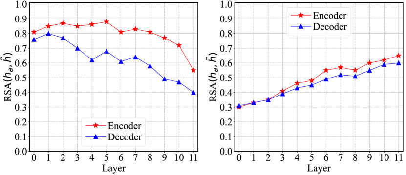
Figure 4: The average RSA similarity of MixPHM between $\boldsymbol{h}_{a}$ and $\boldsymbol{h}$ (left) as well as $\boldsymbol{h}_{a}$ and $\tilde{\boldsymbol{h}}$ (right) at each transformer layer.

Redundancy Analysis of MixPHM.  In this paper, we propose an insight that improving the effectiveness of adapters via reducing task-irrelevant redundancy and promoting task-relevant correlation in representations. To assess whether our method actually leads to performance improvements based on this insight, we conduct the redundancy analysis in the MixPHM representation space under the same experimental settings as described in Sec. 4.1. Figure 4 illustrates the RSA similarity across 1k samples on VQA v2. Compared with the redundancy analysis result of adapter shown in Figure 1, we observe that MixPHM markedly reduces the representation redundancy between $\boldsymbol{h}_{a}$ and $\boldsymbol{h}$, while increasing the representation correlation between $\boldsymbol{h}_{a}$ and $\tilde{\boldsymbol{h}}$. This finding provides a perceptive demonstration for the soundness of our motivation and the effectiveness of our method.

VLMs	Method	#Param	#Sample
		(M)	$N_{\mathcal{D}}$=16	$N_{\mathcal{D}}$=64	$N_{\mathcal{D}}$=500	$N_{\mathcal{D}}$=1000
X-VLM	Finetuning	294	26.63	30.45	38.96	43.92
[60]	MixPHM	0.66	27.54	31.80	41.05	48.06
BLIP	Finetuning	385	27.01	30.05	37.00	42.22
[30]	MixPHM	0.87	29.17	32.09	41.80	46.78
OFA${}_{\text{Base}}$	Finetuning	180	27.48	31.75	42.99	46.81
[53]	MixPHM	0.70	28.46	33.00	45.88	50.01

Table 5: Experimental results of MixPHM on other pretrained VLMs. We report the average VQA-Score across five seeds on VQA v2 validation set under different low-resource settings.

Generalizability to Other Pretrained VLMs.  To demonstrate the generalization capability of our method on other pretrained VLMs, we apply MixPHM to adapt pretrained X-VLM [60], BLIP [30], and OFA${}_{\text{Base}}$ [53] for the low-resource VQA task. Table 5 presents a lite comparison between our method and full finetuning on VQA v2. We observe that MixPHM consistently outperforms full finetuning in all settings, with significant performance gains observed when $N_{\mathcal{D}}$ $\in$ $\{500,1000\}$. Notably, the largest performance gaps from finetuning are achieved by X-VLM (+4.14), BLIP (+4.80), and OFA${}_{\text{Base}}$ (+3.20) at $N_{\mathcal{D}}$=1000, $N_{\mathcal{D}}$=500, and $N_{\mathcal{D}}$=1000, respectively. These findings demonstrate the generalizability of MixPHM to various pretrained VLMs. More comparisons between parameter-efficient methods are available in Appendix C.

6 Conclusion and Limitation

In this paper, we propose a redundancy-aware parameter-efficient tuning method to adapt pretrained VLMs to the low-resource VQA task. The proposed MixPHM reduces task-irrelevant redundancy while promoting task-relevant correlation through a proposed redundancy regularization. Experiments demonstrate its effectiveness and superiority in terms of performance and parameter efficiency.

Redundancy is a double-edged sword. In addition to reducing task-irrelevant redundancy, we can also exploit task-relevant redundancy already learned by pretrained VLMs to enhance performance. Although MixPHM emphasizes reducing task-irrelevant redundancy, there is no explicit guarantee that the reduced redundancy is ineffective for given tasks. As such, a potential prospect is to investigate how to explicitly delimit and minimize task-irrelevant redundancy.

Acknowledgements.  This work was supported by the National Science Foundation of China (Grant No. 62088102).

Appendix

In the Appendix, we provide some supplementary material for our experiments. Specifically, Appendix A explores the impact of different routing mechanisms and hyperparameters on MixPHM. Appendix B presents some visualization results of our method. Appendix C provides additional comparisons between parameter-efficient tuning methods using pretrained X-VLM on VQA v2. Appendix D describes more implementation details.

Appendix A Ablation Study and Parameter Analysis

In this section, using pretrained VL-T5 [5] as the underlying pretrained VLMs, we conduct additional ablation experiments on routing mechanisms and hyperparameter analysis on VQA v2, GQA, and OK-VQA with $N_{\mathcal{D}}=64$.

Impact of Routing Mechanisms.  In MixPHM, in addition to performance, routing mechanisms also affect the training speed, i.e., T/Itr (s). To analyze the impact of different routing strategies on performance and speed, we first introduce two random routing methods, i.e., token-level and sentence-level routing [8]. In addition, we develop a simple representation-based rounding by averaging the outputs of all PHM-experts in each MixPHM. Table 6 shows that random routing mechanism is the fastest and has the best performance on both VQA v2 and OK-VQA.

Impact of Hyperparameters.  To investigate the impact of different hyperparameters on MixPHM, we conduct experiments by varying $N_{e}$, $d_{r}$, $d_{k}$, and $n$. More specifically, we consider the following settings: $N_{e}\in\{1,2,4,8,12\}$, $d_{r}\in\{48,64,96,192\}$, $d_{k}\in\{1,8,16,24\}$, and $n\in\{2,4,8,16\}$. The results in Table 7 show that changing these hyperparameters has only a slight impact on the performance of MixPHM. In addition, the performance of MixPHM with different hyperparameters always outperforms full finetuning. This suggests that the performance improvement brought by MixPHM does not significantly depend on the hyperparameter selection.

Impact of $\alpha$.  When tuning pretrained VLMs with MixPHM, $\alpha$ controls the trade-off between redundancy regularization and generative modeling loss. To investigate the impact of $\alpha$ on MixPHM, we perform experiments with different values of $\alpha$, i.e., $\alpha\in\{0.04,0.06,0.08,0.1,0.2,0.4\}$. Figure 5 illustrates the curve of VQA-Score as $\alpha$ increases. We observe that varying $\alpha$ within a certain range $[0.04,0.4]$ does not hinder the advantage of MixPHM over full finetuning. In addition, according to the results on three datasets, we empirically set $\alpha$ to 0.2.

Method	T/Itr (s)	VQA v2	GQA	OK-VQA
MixPHM-Token	0.693	47.67$\leavevmode\nobreak\ {}_{\pm{0.92}}$	36.23$\leavevmode\nobreak\ {}_{\pm{0.89}}$	17.77$\leavevmode\nobreak\ {}_{\pm{0.89}}$
MixPHM-Sent	0.683	47.69$\leavevmode\nobreak\ {}_{\pm{0.99}}$	36.13$\leavevmode\nobreak\ {}_{\pm{0.86}}$	17.83$\leavevmode\nobreak\ {}_{\pm{1.32}}$
MixPHM-Rep	0.675	48.00$\leavevmode\nobreak\ {}_{\pm{0.95}}$	36.77$\leavevmode\nobreak\ {}_{\pm{0.55}}$	18.25$\leavevmode\nobreak\ {}_{\pm{1.46}}$
MixPHM	0.668	48.26$\leavevmode\nobreak\ {}_{\pm{0.56}}$	36.75$\leavevmode\nobreak\ {}_{\pm{0.55}}$	18.58$\leavevmode\nobreak\ {}_{\pm{1.42}}$

Table 6: Ablation on different routing mechanisms with $N_{\mathcal{D}}=64$. T/Itr (s) is the average tuning time for each iteration.

HP		#Param	VQA v2	GQA	OK-VQA
Finetuning		224.54	46.87$\leavevmode\nobreak\ {}_{\pm{0.57}}$	34.22$\leavevmode\nobreak\ {}_{\pm{0.59}}$	16.65$\leavevmode\nobreak\ {}_{\pm{1.02}}$
	1	0.34	47.30$\leavevmode\nobreak\ {}_{\pm{0.97}}$	36.30$\leavevmode\nobreak\ {}_{\pm{0.83}}$	17.59$\leavevmode\nobreak\ {}_{\pm{0.97}}$
	2	0.52	47.90$\leavevmode\nobreak\ {}_{\pm{0.65}}$	36.88$\leavevmode\nobreak\ {}_{\pm{0.75}}$	18.08$\leavevmode\nobreak\ {}_{\pm{1.28}}$
	4	0.87	48.26$\leavevmode\nobreak\ {}_{\pm{0.56}}$	36.75$\leavevmode\nobreak\ {}_{\pm{0.55}}$	18.58$\leavevmode\nobreak\ {}_{\pm{1.42}}$
	8	1.59	48.09$\leavevmode\nobreak\ {}_{\pm{0.67}}$	36.50$\leavevmode\nobreak\ {}_{\pm{0.81}}$	18.51$\leavevmode\nobreak\ {}_{\pm{1.29}}$
$N_{e}$	12	2.30	47.80$\leavevmode\nobreak\ {}_{\pm{0.72}}$	36.30$\leavevmode\nobreak\ {}_{\pm{0.80}}$	18.43$\leavevmode\nobreak\ {}_{\pm{1.50}}$
	48	0.86	48.36$\leavevmode\nobreak\ {}_{\pm{0.97}}$	36.36$\leavevmode\nobreak\ {}_{\pm{0.32}}$	18.05$\leavevmode\nobreak\ {}_{\pm{0.85}}$
	64	0.87	48.26$\leavevmode\nobreak\ {}_{\pm{0.56}}$	36.75$\leavevmode\nobreak\ {}_{\pm{0.55}}$	18.58$\leavevmode\nobreak\ {}_{\pm{1.42}}$
	96	0.91	48.05$\leavevmode\nobreak\ {}_{\pm{0.82}}$	36.36$\leavevmode\nobreak\ {}_{\pm{0.51}}$	18.39$\leavevmode\nobreak\ {}_{\pm{0.96}}$
$d_{r}$	192	1.00	47.97$\leavevmode\nobreak\ {}_{\pm{1.17}}$	36.37$\leavevmode\nobreak\ {}_{\pm{0.82}}$	18.26$\leavevmode\nobreak\ {}_{\pm{1.20}}$
	1	0.18	47.87$\leavevmode\nobreak\ {}_{\pm{0.73}}$	35.74$\leavevmode\nobreak\ {}_{\pm{0.70}}$	17.04$\leavevmode\nobreak\ {}_{\pm{0.81}}$
	8	0.87	48.26$\leavevmode\nobreak\ {}_{\pm{0.56}}$	36.75$\leavevmode\nobreak\ {}_{\pm{0.55}}$	18.58$\leavevmode\nobreak\ {}_{\pm{1.70}}$
	16	1.67	48.35$\leavevmode\nobreak\ {}_{\pm{1.14}}$	36.62$\leavevmode\nobreak\ {}_{\pm{0.35}}$	18.22$\leavevmode\nobreak\ {}_{\pm{1.36}}$
$d_{k}$	24	2.47	48.07$\leavevmode\nobreak\ {}_{\pm{1.12}}$	36.42$\leavevmode\nobreak\ {}_{\pm{0.52}}$	18.79$\leavevmode\nobreak\ {}_{\pm{1.18}}$
	2	0.87	48.17$\leavevmode\nobreak\ {}_{\pm{0.93}}$	36.53$\leavevmode\nobreak\ {}_{\pm{0.32}}$	18.43$\leavevmode\nobreak\ {}_{\pm{0.75}}$
	4	0.87	48.26$\leavevmode\nobreak\ {}_{\pm{0.56}}$	36.75$\leavevmode\nobreak\ {}_{\pm{0.55}}$	18.58$\leavevmode\nobreak\ {}_{\pm{1.42}}$
	8	0.87	47.97$\leavevmode\nobreak\ {}_{\pm{1.08}}$	36.37$\leavevmode\nobreak\ {}_{\pm{0.56}}$	17.41$\leavevmode\nobreak\ {}_{\pm{1.05}}$
$n$	16	0.88	46.65$\leavevmode\nobreak\ {}_{\pm{1.10}}$	35.46$\leavevmode\nobreak\ {}_{\pm{0.55}}$	17.52$\leavevmode\nobreak\ {}_{\pm{0.63}}$

Table 7: Impact of hyperparameters (HP) on MixPHM. $N_{e}$: the number of PHM-experts, $d_{r}$: bottleneck dimension, $d_{k}$: rank dimension, $n$: the number of summations of Kronecker product.

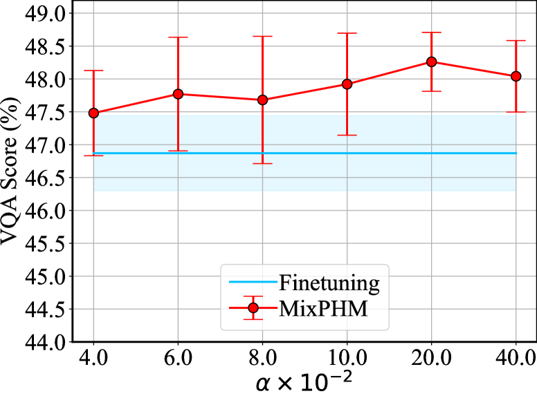
(a) VQA v2

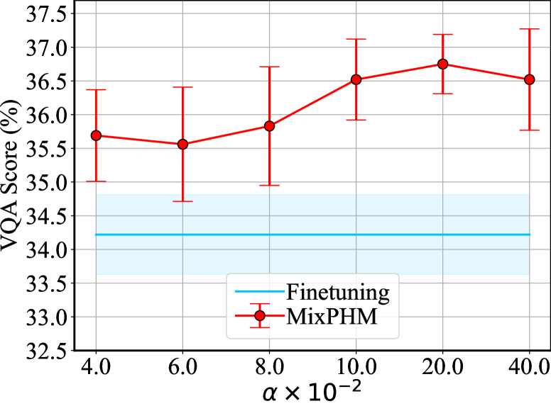
(b) GQA

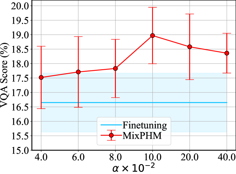
(c) OK-VQA

Figure 5: The average VQA-Score with standard deviation across five seeds as $\alpha$ varies.

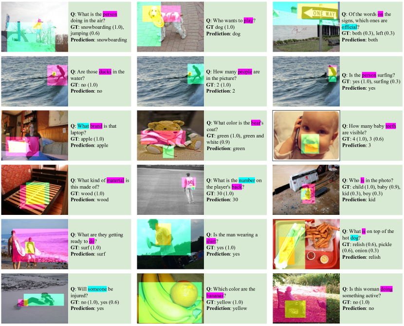
Figure 6: Qualitative results on VQA v2 validation set. The Prediction is generated by the VL-T5 tuned with the proposed MixPHM. GT denotes the annotated answer and the corresponding score. We visualize the top-down attention [1] of images and mark the task-relevant tokens of questions for the first and second highest attention scores.

Method	#Param		#Sample
	(M)	(%)	$N_{\mathcal{D}}$=16	$N_{\mathcal{D}}$=32	$N_{\mathcal{D}}$=64	$N_{\mathcal{D}}$=100	$N_{\mathcal{D}}$=500	$N_{\mathcal{D}}$=1,000
Finetuning	293.48	100%	26.63$\leavevmode\nobreak\ {}_{\pm{0.98}}$	29.33$\leavevmode\nobreak\ {}_{\pm{1.68}}$	30.45$\leavevmode\nobreak\ {}_{\pm{1.80}}$	31.48$\leavevmode\nobreak\ {}_{\pm{1.57}}$	38.96$\leavevmode\nobreak\ {}_{\pm{1.56}}$	43.92$\leavevmode\nobreak\ {}_{\pm{1.22}}$
BitFit [59]	0.29	0.13%	25.48$\leavevmode\nobreak\ {}_{\pm{3.81}}$	28.90$\leavevmode\nobreak\ {}_{\pm{1.14}}$	30.73$\leavevmode\nobreak\ {}_{\pm{1.18}}$	31.92$\leavevmode\nobreak\ {}_{\pm{1.14}}$	36.77$\leavevmode\nobreak\ {}_{\pm{1.32}}$	40.77$\leavevmode\nobreak\ {}_{\pm{0.79}}$
LoRA [17]	0.37	0.13%	25.31$\leavevmode\nobreak\ {}_{\pm{1.50}}$	26.91$\leavevmode\nobreak\ {}_{\pm{3.09}}$	30.52$\leavevmode\nobreak\ {}_{\pm{1.67}}$	31.97$\leavevmode\nobreak\ {}_{\pm{1.11}}$	36.13$\leavevmode\nobreak\ {}_{\pm{1.12}}$	40.49$\leavevmode\nobreak\ {}_{\pm{0.87}}$
Compacter [24]	0.25	0.09%	25.69$\leavevmode\nobreak\ {}_{\pm{2.34}}$	28.04$\leavevmode\nobreak\ {}_{\pm{1.63}}$	28.10$\leavevmode\nobreak\ {}_{\pm{2.06}}$	31.35$\leavevmode\nobreak\ {}_{\pm{0.34}}$	35.91$\leavevmode\nobreak\ {}_{\pm{0.65}}$	40.44$\leavevmode\nobreak\ {}_{\pm{0.77}}$
Houlsby [16]	3.57	1.20%	26.54$\leavevmode\nobreak\ {}_{\pm{2.57}}$	29.34$\leavevmode\nobreak\ {}_{\pm{2.25}}$	30.74$\leavevmode\nobreak\ {}_{\pm{1.20}}$	31.71$\leavevmode\nobreak\ {}_{\pm{1.43}}$	38.48$\leavevmode\nobreak\ {}_{\pm{0.91}}$	41.96$\leavevmode\nobreak\ {}_{\pm{0.72}}$
Pfeiffer [41]	1.78	0.60%	26.57$\leavevmode\nobreak\ {}_{\pm{2.00}}$	28.46$\leavevmode\nobreak\ {}_{\pm{1.74}}$	29.22$\leavevmode\nobreak\ {}_{\pm{2.56}}$	31.95$\leavevmode\nobreak\ {}_{\pm{1.34}}$	37.39$\leavevmode\nobreak\ {}_{\pm{0.73}}$	40.96$\leavevmode\nobreak\ {}_{\pm{1.09}}$
AdaMix [54]	4.44	1.49%	26.11$\leavevmode\nobreak\ {}_{\pm{1.58}}$	28.91$\leavevmode\nobreak\ {}_{\pm{1.36}}$	30.71$\leavevmode\nobreak\ {}_{\pm{2.05}}$	31.15$\leavevmode\nobreak\ {}_{\pm{1.26}}$	38.48$\leavevmode\nobreak\ {}_{\pm{1.53}}$	43.26$\leavevmode\nobreak\ {}_{\pm{0.85}}$
MixPHM	0.66	0.22%	27.54$\leavevmode\nobreak\ {}_{\pm{1.52}}$	30.65$\leavevmode\nobreak\ {}_{\pm{1.09}}$	31.80$\leavevmode\nobreak\ {}_{\pm{1.61}}$	32.58$\leavevmode\nobreak\ {}_{\pm{1.09}}$	41.05$\leavevmode\nobreak\ {}_{\pm{1.22}}$	48.06$\leavevmode\nobreak\ {}_{\pm{0.64}}$

Table 8: Experimental results with pretrained X-VLM. The average VQA-Score with standard deviation across 5 different seeds are evaluated on VQA v2 validation set. The best and second best parameter-efficient tuning methods are highlighted. The number of tuned parameters and the percentage of tuned parameters relative to X-VLM (i.e., 293.48M) are reported.

Appendix B Visualization Results

We visualize some examples of the proposed MixPHM. As depicted in Figure 6, these predictions are generated by the VL-T5 tuned with MixPHM on VQA v2 with $N_{\mathcal{D}}=64$. In addition, we visualize the top-down attention [1] for images and mark the top two task-relevant tokens for questions. More specifically, we follow a recent work [22] to compute an attention score between task-relevant representations and visual input features obtained using bottom-up Faster R-CNN [1] and visualize the top-down attention for the first and second highest scores. Analogously, we compute the score between task-relevant representations and linguistic embeddings of questions and mark the tokens for the first and second highest scores. Figure 6 qualitatively shows that our MixPHM can generate consistent and question-relevant visual and textual attentions in the process of answer prediction.

Appendix C Results with Pretrained X-VLM

As a supplement to the results in Table 5 of the main paper, we utilize pretrained X-VLM [60] as a representative and compare our methods with state-of-the-art parameter-efficient tuning methods on VQA v2 validation set. The key hyperparameter settings for these parameter-efficient methods are the same as those in Table 9. The conclusions that we observe in Table 8 are consistent with Table 5, i.e., our method consistently outperforms existing parameter-efficient tuning methods when using other pretrained VLMs, which further demonstrates the generalization capability of MixPHM.

Appendix D Implementation Details

For parameter-efficient tuning methods, we search the bottleneck dimension $d_{r}$ from $\{48,64,96,192\}$ for all adapter-based methods (i.e., MixPHM, AdaMix, Pfeiffer, Houlsby and Compacter), the number of experts $N_{e}$ from $\{1,2,4,8,12\}$ for MixPHM and AdaMix, the rank dimension $d_{r}$ (for MixPHM and Compacter), $r$ (for LoRA) from $\{1,8,16,24\}$, as well as the number of summations of Kronecker product $n$ from $\{2,4,8,16\}$ for MixPHM and Compacter. Table 9 presents the final configuration of the hyperparameters used in our experiments. For MixPHM, we set the trade-off factor $\alpha$ to 0.2.

All methods are implemented using Pytorch [39] on an NVIDIA GeForce RTX 3090Ti GPU. In addition, we also perform a grid search to select the best learning rate from $\{5\times 10^{-5},1\times 10^{-4},5\times 10^{-4},1\times 10^{-3},5\times 10^{-3}\}$. The batch size and the number of epochs are set to 16 and 1000, respectively. We utilize AdamW optimizer [34] and the early stopping strategy with a patience of 200 non-increasing epochs, where the stopping metric is the VQA-Score on the development set $\mathcal{D}_{\text{dev}}$ of datasets.

Method	Learning rate	Configuration
Finetuning	$5\times 10^{-5}$	—
BitFit	$5\times 10^{-5}$	—
LoRA	$5\times 10^{-5}$	$r=4$
Compacter	$5\times 10^{-3}$	$d_{r}=64$, $d_{k}=8$, $n=4$
Houlsby	$5\times 10^{-5}$	$d_{r}=64$
Pfeiffer	$5\times 10^{-5}$	$d_{r}=64$
AdaMix	$5\times 10^{-4}$	$N_{e}=4$, $d_{r}=64$
MixPHM	$5\times 10^{-3}$	$N_{e}=4$, $d_{r}=64$, $d_{k}=8$, $n=4$

Table 9: Hyperparameter settings for all parameter-efficient tuning methods. $N_{e}$: the number of experts, $d_{r}$: bottleneck dimension, $d_{k}$ and $r$: rank dimension, $n$: the number of summations of Kronecker product.

References

- [1] Peter Anderson, Xiaodong He, Chris Buehler, Damien Teney, Mark Johnson, Stephen Gould, and Lei Zhang. Bottom-up and top-down attention for image captioning and visual question answering. In CVPR, pages 6077–6086, 2018.
- [2] Stanislaw Antol, Aishwarya Agrawal, Jiasen Lu, Margaret Mitchell, Dhruv Batra, C Lawrence Zitnick, and Devi Parikh. Vqa: Visual question answering. In ICCV, pages 2425–2433, 2015.
- [3] Tom Brown, Benjamin Mann, Nick Ryder, Melanie Subbiah, Jared D Kaplan, Prafulla Dhariwal, Arvind Neelakantan, Pranav Shyam, Girish Sastry, Amanda Askell, et al. Language models are few-shot learners. In NeurIPS, pages 1877–1901, 2020.
- [4] Guanzheng Chen, Fangyu Liu, Zaiqiao Meng, and Shangsong Liang. Revisiting parameter-efficient tuning: Are we really there yet? In EMNLP, pages 2612–2626, 2022.
- [5] Jaemin Cho, Jie Lei, Hao Tan, and Mohit Bansal. Unifying vision-and-language tasks via text generation. In ICML, pages 1931–1942, 2021.
- [6] Zi-Yi Dou, Yichong Xu, Zhe Gan, Jianfeng Wang, Shuohang Wang, Lijuan Wang, Chenguang Zhu, Pengchuan Zhang, Lu Yuan, Nanyun Peng, et al. An empirical study of training end-to-end vision-and-language transformers. In CVPR, pages 18166–18176, 2022.
- [7] Nan Du, Yanping Huang, Andrew M Dai, Simon Tong, Dmitry Lepikhin, Yuanzhong Xu, Maxim Krikun, Yanqi Zhou, Adams Wei Yu, Orhan Firat, et al. Glam: Efficient scaling of language models with mixture-of-experts. In ICML, pages 5547–5569, 2022.
- [8] William Fedus, Barret Zoph, and Noam Shazeer. Switch transformers: Scaling to trillion parameter models with simple and efficient sparsity. arXiv preprint arXiv:2101.03961, 2021.
- [9] Zhe Gan, Yen-Chun Chen, Linjie Li, Chen Zhu, Yu Cheng, and Jingjing Liu. Large-scale adversarial training for vision-and-language representation learning. In NeurIPS, 2020.
- [10] Tianyu Gao, Adam Fisch, and Danqi Chen. Making pre-trained language models better few-shot learners. In ACL, pages 3816–3830, 2021.
- [11] Ze-Feng Gao, Peiyu Liu, Wayne Xin Zhao, Zhong-Yi Lu, and Ji-Rong Wen. Parameter-efficient mixture-of-experts architecture for pre-trained language models. In COLING, pages 3263–3273, 2022.
- [12] Yash Goyal, Tejas Khot, Douglas Summers-Stay, Dhruv Batra, and Devi Parikh. Making the v in vqa matter: Elevating the role of image understanding in visual question answering. In CVPR, pages 6904–6913, 2017.
- [13] Junxian He, Chunting Zhou, Xuezhe Ma, Taylor Berg-Kirkpatrick, and Graham Neubig. Towards a unified view of parameter-efficient transfer learning. In ICLR, 2022.
- [14] Ruidan He, Linlin Liu, Hai Ye, Qingyu Tan, Bosheng Ding, Liying Cheng, Jia-Wei Low, Lidong Bing, and Luo Si. On the effectiveness of adapter-based tuning for pretrained language model adaptation. In ACL, pages 2208–2222, 2021.
- [15] R Devon Hjelm, Alex Fedorov, Samuel Lavoie-Marchildon, Karan Grewal, Phil Bachman, Adam Trischler, and Yoshua Bengio. Learning deep representations by mutual information estimation and maximization. In ICLR, 2019.
- [16] Neil Houlsby, Andrei Giurgiu, Stanislaw Jastrzebski, Bruna Morrone, Quentin De Laroussilhe, Andrea Gesmundo, Mona Attariyan, and Sylvain Gelly. Parameter-efficient transfer learning for nlp. In ICML, pages 2790–2799, 2019.
- [17] Edward J Hu, Yelong Shen, Phillip Wallis, Zeyuan Allen-Zhu, Yuanzhi Li, Shean Wang, Lu Wang, and Weizhu Chen. Lora: Low-rank adaptation of large language models. In ICLR, 2022.
- [18] Ronghang Hu and Amanpreet Singh. Unit: Multimodal multitask learning with a unified transformer. In ICCV, pages 1439–1449, 2021.
- [19] Zhicheng Huang, Zhaoyang Zeng, Yupan Huang, Bei Liu, Dongmei Fu, and Jianlong Fu. Seeing out of the box: End-to-end pre-training for vision-language representation learning. In CVPR, pages 12976–12985, 2021.
- [20] Drew A Hudson and Christopher D Manning. GQA: A new dataset for real-world visual reasoning and compositional question answering. In CVPR, pages 6700–6709, 2019.
- [21] Chao Jia, Yinfei Yang, Ye Xia, Yi-Ting Chen, Zarana Parekh, Hieu Pham, Quoc Le, Yun-Hsuan Sung, Zhen Li, and Tom Duerig. Scaling up visual and vision-language representation learning with noisy text supervision. In ICML, pages 4904–4916, 2021.
- [22] Jingjing Jiang, Ziyi Liu, and Nanning Zheng. Correlation information bottleneck: Towards adapting pretrained multimodal models for robust visual question answering. arXiv preprint arXiv:2209.06954, 2022.
- [23] Woojeong Jin, Yu Cheng, Yelong Shen, Weizhu Chen, and Xiang Ren. A good prompt is worth millions of parameters: Low-resource prompt-based learning for vision-language models. In ACL, pages 2763–2775, 2022.
- [24] Rabeeh Karimi Mahabadi, James Henderson, and Sebastian Ruder. Compacter: Efficient low-rank hypercomplex adapter layers. In NeurIPS, pages 1022–1035, 2021.
- [25] Wonjae Kim, Bokyung Son, and Ildoo Kim. Vilt: Vision-and-language transformer without convolution or region supervision. In ICML, pages 5583–5594, 2021.
- [26] Aarre Laakso and Garrison Cottrell. Content and cluster analysis: Assessing representational similarity in neural systems. Philosophical Psychology, 13(1):47–76, 2000.
- [27] Dmitry Lepikhin, HyoukJoong Lee, Yuanzhong Xu, Dehao Chen, Orhan Firat, Yanping Huang, Maxim Krikun, Noam Shazeer, and Zhifeng Chen. Gshard: Scaling giant models with conditional computation and automatic sharding. In ICLR, 2021.
- [28] Brian Lester, Rami Al-Rfou, and Noah Constant. The power of scale for parameter-efficient prompt tuning. In EMNLP, pages 3045–3059, 2021.
- [29] Mike Lewis, Shruti Bhosale, Tim Dettmers, Naman Goyal, and Luke Zettlemoyer. Base layers: Simplifying training of large, sparse models. In ICML, pages 6265–6274, 2021.
- [30] Junnan Li, Dongxu Li, Caiming Xiong, and Steven Hoi. Blip: Bootstrapping language-image pre-training for unified vision-language understanding and generation. In ICML, pages 12888–12900, 2022.
- [31] Junnan Li, Ramprasaath Selvaraju, Akhilesh Gotmare, Shafiq Joty, Caiming Xiong, and Steven Chu Hong Hoi. Align before fuse: Vision and language representation learning with momentum distillation. In NeurIPS, pages 9694–9705, 2021.
- [32] Xiang Lisa Li and Percy Liang. Prefix-tuning: Optimizing continuous prompts for generation. In ACL, pages 4582–4597, 2021.
- [33] Bingqian Lin, Yi Zhu, Zicong Chen, Xiwen Liang, Jianzhuang Liu, and Xiaodan Liang. Adapt: Vision-language navigation with modality-aligned action prompts. In CVPR, pages 15396–15406, 2022.
- [34] Ilya Loshchilov and Frank Hutter. Decoupled weight decay regularization. In ICLR, 2019.
- [35] Rabeeh Karimi Mahabadi, Yonatan Belinkov, and James Henderson. Variational information bottleneck for effective low-resource fine-tuning. In ICLR, 2021.
- [36] Rabeeh Karimi Mahabadi, Sebastian Ruder, Mostafa Dehghani, and James Henderson. Parameter-efficient multi-task fine-tuning for transformers via shared hypernetworks. In ACL, pages 565–576, 2021.
- [37] Yuning Mao, Lambert Mathias, Rui Hou, Amjad Almahairi, Hao Ma, Jiawei Han, Scott Yih, and Madian Khabsa. Unipelt: A unified framework for parameter-efficient language model tuning. In ACL, pages 6253–6264, 2022.
- [38] Kenneth Marino, Mohammad Rastegari, Ali Farhadi, and Roozbeh Mottaghi. Ok-vqa: A visual question answering benchmark requiring external knowledge. In CVPR, pages 3195–3204, 2019.
- [39] Adam Paszke, Sam Gross, Francisco Massa, Adam Lerer, James Bradbury, Gregory Chanan, Trevor Killeen, Zeming Lin, Natalia Gimelshein, Luca Antiga, et al. Pytorch: An imperative style, high-performance deep learning library. In NeurIPS, pages 8024–8035, 2019.
- [40] Ethan Perez, Douwe Kiela, and Kyunghyun Cho. True few-shot learning with language models. In NeurIPS, pages 11054–11070, 2021.
- [41] Jonas Pfeiffer, Aishwarya Kamath, Andreas Rücklé, Kyunghyun Cho, and Iryna Gurevych. Adapterfusion: Non-destructive task composition for transfer learning. arXiv preprint arXiv:2005.00247, 2020.
- [42] Carlos Riquelme, Joan Puigcerver, Basil Mustafa, Maxim Neumann, Rodolphe Jenatton, André Susano Pinto, Daniel Keysers, and Neil Houlsby. Scaling vision with sparse mixture of experts. In NeurIPS, pages 8583–8595, 2021.
- [43] Stephen Roller, Sainbayar Sukhbaatar, Jason Weston, et al. Hash layers for large sparse models. In NeurIPS, pages 17555–17566, 2021.
- [44] Andreas Rücklé, Gregor Geigle, Max Glockner, Tilman Beck, Jonas Pfeiffer, Nils Reimers, and Iryna Gurevych. Adapterdrop: On the efficiency of adapters in transformers. In EMNLP, pages 7930–7946, 2021.
- [45] Noam Shazeer, Azalia Mirhoseini, Krzysztof Maziarz, Andy Davis, Quoc Le, Geoffrey Hinton, and Jeff Dean. Outrageously large neural networks: The sparsely-gated mixture-of-experts layer. In ICLR, 2017.
- [46] Yi-Lin Sung, Jaemin Cho, and Mohit Bansal. VL-adapter: Parameter-efficient transfer learning for vision-and-language tasks. In CVPR, pages 5227–5237, 2022.
- [47] Yi-Lin Sung, Varun Nair, and Colin A Raffel. Training neural networks with fixed sparse masks. In NeurIPS, pages 24193–24205, 2021.
- [48] Hao Tan and Mohit Bansal. LXMERT: Learning cross-modality encoder representations from transformers. In EMNLP, pages 5099–5110, 2019.
- [49] Naftali Tishby and Noga Zaslavsky. Deep learning and the information bottleneck principle. arXiv preprint arXiv:1503.02406, 2015.
- [50] Maria Tsimpoukelli, Jacob Menick, Serkan Cabi, SM Eslami, Oriol Vinyals, and Felix Hill. Multimodal few-shot learning with frozen language models. In NeurIPS, pages 200–212, 2021.
- [51] Boxin Wang, Shuohang Wang, Yu Cheng, Zhe Gan, Ruoxi Jia, Bo Li, and Jingjing Liu. InfoBERT: Improving robustness of language models from an information theoretic perspective. In ICLR, 2021.
- [52] Haoqing Wang, Xun Guo, Zhi-Hong Deng, and Yan Lu. Rethinking minimal sufficient representation in contrastive learning. In CVPR, pages 16041–16050, 2022.
- [53] Peng Wang, An Yang, Rui Men, Junyang Lin, Shuai Bai, Zhikang Li, Jianxin Ma, Chang Zhou, Jingren Zhou, and Hongxia Yang. OFA: Unifying architectures, tasks, and modalities through a simple sequence-to-sequence learning framework. In ICML, pages 23318–23340, 2022.
- [54] Yaqing Wang, Subhabrata Mukherjee, Xiaodong Liu, Jing Gao, Ahmed Hassan Awadallah, and Jianfeng Gao. Adamix: Mixture-of-adapter for parameter-efficient tuning of large language models. In EMNLP, pages 5744–5760, 2022.
- [55] Zirui Wang, Jiahui Yu, Adams Wei Yu, Zihang Dai, Yulia Tsvetkov, and Yuan Cao. Simvlm: Simple visual language model pretraining with weak supervision. In ICLR, 2022.
- [56] Mitchell Wortsman, Gabriel Ilharco, Samir Ya Gadre, Rebecca Roelofs, Raphael Gontijo-Lopes, Ari S Morcos, Hongseok Namkoong, Ali Farhadi, Yair Carmon, Simon Kornblith, et al. Model soups: averaging weights of multiple fine-tuned models improves accuracy without increasing inference time. In ICML, pages 23965–23998, 2022.
- [57] Zhengyuan Yang, Zhe Gan, Jianfeng Wang, Xiaowei Hu, Yumao Lu, Zicheng Liu, and Lijuan Wang. An empirical study of gpt-3 for few-shot knowledge-based vqa. In AAAI, pages 3081–3089, 2022.
- [58] Zonghan Yang and Yang Liu. On robust prefix-tuning for text classification. In ICLR, 2022.
- [59] Elad Ben Zaken, Shauli Ravfogel, and Yoav Goldberg. Bitfit: Simple parameter-efficient fine-tuning for transformer-based masked language-models. In ACL, pages 1–9, 2022.
- [60] Yan Zeng, Xinsong Zhang, and Hang Li. Multi-grained vision language pre-training: Aligning texts with visual concepts. In ICML, pages 25994–26009, 2022.
- [61] Aston Zhang, Yi Tay, Shuai Zhang, Alvin Chan, Anh Tuan Luu, Siu Cheung Hui, and Jie Fu. Beyond fully-connected layers with quaternions: Parameterization of hypercomplex multiplications with parameters. In ICLR, 2021.
- [62] Ningyu Zhang, Luoqiu Li, Xiang Chen, Shumin Deng, Zhen Bi, Chuanqi Tan, Fei Huang, and Huajun Chen. Differentiable prompt makes pre-trained language models better few-shot learners. In ICLR, 2022.
- [63] Pengchuan Zhang, Xiujun Li, Xiaowei Hu, Jianwei Yang, Lei Zhang, Lijuan Wang, Yejin Choi, and Jianfeng Gao. Vinvl: Revisiting visual representations in vision-language models. In CVPR, pages 5579–5588, 2021.
- [64] Zhengkun Zhang, Wenya Guo, Xiaojun Meng, Yasheng Wang, Yadao Wang, Xin Jiang, Qun Liu, and Zhenglu Yang. Hyperpelt: Unified parameter-efficient language model tuning for both language and vision-and-language tasks. arXiv preprint arXiv:2203.03878, 2022.
- [65] Yiwu Zhong, Jianwei Yang, Pengchuan Zhang, Chunyuan Li, Noel Codella, Liunian Harold Li, Luowei Zhou, Xiyang Dai, Lu Yuan, Yin Li, et al. Regionclip: Region-based language-image pretraining. In CVPR, pages 16793–16803, 2022.
- [66] Simiao Zuo, Xiaodong Liu, Jian Jiao, Young Jin Kim, Hany Hassan, Ruofei Zhang, Tuo Zhao, and Jianfeng Gao. Taming sparsely activated transformer with stochastic experts. In ICLR, 2022.