Generation of intraparticle quantum correlations in amplitude damping channel and its robustness

Abstract

Quantum correlations between two or more different degrees of freedom of the same particle is sometimes referred to as intraparticle entanglement. In this work, we study these intra-particle correlations between two different degrees of freedom under various decoherence channels viz. amplitude damping, depolarising and phase damping channels. We observe a unique feature of the amplitude damping channel, wherein entanglement is shown to arise starting from separable states. In case of non maximally entangled input states, in addition to entanglement sudden death, the creation of entanglement is also observed, having an asymptotic decay over a long time. These counter-intuitive behaviours arise due to the subtle interplay of channel and input state parameters, and are not seen for interparticle entanglement without consideration of non-Markovian noise. It is also not observed for maximally entangled input states. Furthermore, investigation of entanglement evolution in phase damping and depolarizing channels shows its robustness against decoherence as compared to interparticle entanglement.

I Introduction

Entanglement can arise between two spatially separated particles or two different degrees of freedom of the same particle due to the nonseparability of the states in the Hilbert space. Interparticle entanglement refers to nonlocal quantum correlations between two spatially separated particles that violate the Bell-CHSH inequality Bell1964 ; CHSH , which comes from the assumption of realism and locality. On the other hand, a single system with intraparticle correlations, sometimes also referred to as intraparticle entanglement, violates a Bell-CHSH like inequality Basu , derived from the assumption of noncontextuality Kochen . Intraparticle entanglement has been experimentally verified for various quantum systems Michler2000 ; Gadway2009 ; Mair2001 ; Barreiro2005 ; Hasegawa2003 ; Shen2020 . It is an important resource for the testing of quantum contextuality and its applications, such as quantum key distribution protocols Sun2011 ; Adhikari2015 , quantum teleportation protocols Heo2015 ; Pramanik2010 ; Hong2015 , entanglement swapping protocols Adhikari2010 .

Any real-life applications of entanglement would suffer from interactions with a noisy environment. Thus, for realistic applications, it is imperative to investigate the nature of intraparticle entanglement in noisy channels. Further, for finding its efficacy, the same should be contrasted and compared with the decohering effects of noisy channels on interparticle entanglement, which have been systematically studied Yu2009 ; Alm2007 ; Almeida2008 . In this work, we extensively study the effects of noisy channels, viz. amplitude damping, phase damping and depolarising channels on the intraparticle correlations shared between degrees of freedom of a single particle.

We make use of the Kraus operator formalism, where the evolution of an initial state $\rho$ is described by a trace preserving map $\rho\rightarrow\rho^{{}^{\prime}}=\sum_{i}M_{i}\rho M_{i}^{\dagger}$. ${M}_{i}$ are the Kraus operators satisfying the completeness relation $\sum_{i}M_{i}^{\dagger}M_{i}=\mathcal{I}$.

We consider a single quantum system $S$ with two different degrees of freedom, say $A$ and $B$ whose states belong to two dimensional Hilbert spaces $\mathcal{H}_{A}$ and $\mathcal{H}_{B}$ with orthonormal bases $\{|a_{1}\rangle$, $|a_{2}\rangle\}$ and $\{|b_{1}\rangle$, $|b_{2}\rangle\}$ respectively:

$$|\psi\rangle_{in}=a|a_{1}b_{1}\rangle+b|a_{1}b_{2}\rangle+c|a_{2}b_{1}\rangle+d|a_{2}b_{2}\rangle$$ (1)

with $|a|^{2}+|b|^{2}+|c|^{2}+|d|^{2}=1$. The intraparticle entanglement between two degrees of freedom can be measured by calculating the Concurrence measure, $C=2|ad-bc|$ Wootters1998 . For two spatially separated particles $A$ and $B$, whose states belong to two dimensional Hilbert spaces $H_{A}$ and $H_{B}$ respectively, with orthonormal bases $\{|a_{1}\rangle$, $|a_{2}\rangle\}$ and $\{|b_{1}\rangle$, $|b_{2}\rangle\}$, a general pure state of the joint system $AB$ takes the same mathematical form as well and hence has an identical value of the concurrence. However, the evolution of the concurrence may show significant differences depending on the decoherence of the respective channels. The decoherence of an interparticle entangled state is studied using the Kraus operator formalism KarlKraus ; Almeida2008 , where the effect of the environment acts locally on each particle. In this case, the dimension of the Kraus operators is the same as the dimension of the Hilbert space of the state of each particle. On the other hand, for an intraparticle entangled state of a single particle, both degrees of freedom belong to the same particle. Hence, it is natural to consider that environment acts on both the degrees of freedom of the single particle simultaneously and the dimension of Kraus operators will then be the same as the dimension of the Hilbert space of the state of the particle. Since, an intraparticle entangled state of a particle belongs to a $4$ dimensional Hilbert space, the Kraus operators representing noise will be $4$ dimensional.

The manuscript is organised as follows. We begin by analysing the amplitude damping channel, for which the concurrence is computed as a function of the channel and input state parameters. This reveals the physical origin of entanglement generation starting from separable intraparticle degrees of freedom. Subsequently the causes of entanglement sudden death (ESD) and its regeneration for non maximally entangled input states are explicitly identified. This counter-intuitive behaviour is not seen for interparticle entanglement, without a consideration of non-Markovian noise BBellomo . It is also not seen for maximally entangled states in both the intra and interparticle scenarios. Next, the decoherence of intraparticle entanglement in the phase damping and depolarizing channels are investigated and this is contrasted with the interparticle entanglement scenario to demonstrate the robustness of intraparticle entanglement. The counter-intuitive behaviour of intraparticle entanglement is explained through an explicit analysis of the concurrence in terms of the channel and input state parameters.

Concurrence Wootters1998 is a widely used measure of quantum entanglement. For an arbitrary bipartite quantum state $\rho$, the Concurrence is defined as

$$C(\rho)=max\{0,\sqrt{\lambda_{1}}-\sqrt{\lambda_{2}}-\sqrt{\lambda_{3}}-\sqrt{\lambda_{4}}\}$$ (2)

where the quantities $\lambda_{i}$ are the eigenvalues in decreasing order of the matrix:

$$R=\rho(\sigma_{y}\otimes\sigma_{y})\rho^{*}(\sigma_{y}\otimes\sigma_{y}).$$ (3)

Here $\rho^{*}$ is the complex conjugate of the matrix representing the input state $\rho$ and $\sigma_{y}$ is the Pauli matrix,

$$\sigma_{y}=\begin{pmatrix}0&-i\\ i&0\end{pmatrix}.$$

In the following section, we will calculate all eigenvalues $\lambda_{i}$ of the matrix $R$ for the amplitude damping and phase damping channels as well as for the depolarizing channel and investigate their behaviour systematically for a physical understanding of the entanglement generation and its sudden death. In particular we carefully investigate the origin of differences in entanglement evolution for intra and interparticle cases. The amplitude damping channel is discussed in detail as it exhibits counter-intutive behaviour. This intriguing behaviour enables the amplitude damping channel to behave as a resource as it leads to both entanglement generation as well as a delay in the onset of ESD. This is not observed in the case of interparticle entanglement wherein further approximations like a non-Markovian environment are needed.

II Amplitude damping channel

The amplitude damping channel represents a physical system that dissipates energy to its environment via interaction. The effect of amplitude damping noise on an intraparticle entangled state $|\psi\rangle_{in}$ can be represented by the following Kraus operators ArijitDutta ; AlejandroFonseca

$$M_{0} = |0\rangle\langle 0|+\sqrt{1-P}\sum_{j=1}^{3}|j\rangle\langle j|~{},$$

$$M_{i} = \sqrt{P}|0\rangle\langle i|~{}~{}(i=1,2,3)$$

where $P$ is the channel parameter. After the evolution of $|\psi\rangle_{in}$ through the amplitude damping channel, the final state becomes

$$\rho_{out}=\begin{pmatrix}a^{2}q+P&ab\sqrt{q}&ac\sqrt{q}&ad\sqrt{q}\\ ab\sqrt{q}&b^{2}q&bcq&bdq\\ ac\sqrt{q}&bcq&c^{2}q&cdq\\ ad\sqrt{q}&bdq&cdq&d^{2}q\end{pmatrix}$$ (4)

where $q=1-P$. Next, we calculate the matrix $R$ [Eq. (3)] and find that only two of the eigenvalues of $R$ are nonzero. They are

$$\lambda_{1} = \alpha+(1-P)\sqrt{\beta}$$

$$\lambda_{2} = \alpha-(1-P)\sqrt{\beta}$$ (5)

where

$$\alpha = 2a^{2}d^{2}+2b^{2}c^{2}-4abcd(1-P)^{3/2}+\{(1-3a^{2})d^{2}$$

$$-4b^{2}c^{2}\}P-\{(1-a^{2})d^{2}-2b^{2}c^{2}\}P^{2}~{}~{},$$

$$\beta = \Big{\{}2(bc\sqrt{(1-P)}-ad)^{2}+(1-a^{2})d^{2}P\Big{\}}^{2}$$ (6)

$$-(1-a^{2})^{2}d^{4}P^{2}~{}.$$

When $P=0$, i.e. there is no effect of the amplitude damping channel, $\alpha=2(ad-bc)^{2}$, $\beta=4(ad-bc)^{4}$ and $\alpha=\sqrt{\beta}$. As a result,

$$\lambda_{1} = \alpha+\sqrt{\beta}=2(ad-bc)^{2}+2(ad-bc)^{2}=4(ad-bc)^{2}$$

$$\lambda_{2} = \alpha-\sqrt{\beta}=2(ad-bc)^{2}-2(ad-bc)^{2}=0$$

Thus, at $P=0$, only $\lambda_{1}$ contributes to the expression of the concurrence , i.e., $C=\sqrt{\lambda_{1}}=2|(ad-bc)|$, while other eigenvalues have no contribution. As $P$ increases, we observe that the quantity $\beta$ first increases and then decreases with the increase of $P$. At a particular point $P=1-\frac{a^{2}d^{2}}{b^{2}c^{2}}$, the term $(bc\sqrt{(1-P)}-ad)^{2}$ in the expression of $\beta$ becomes zero and $\beta$ itself also becomes zero.

Depending on the values of the input state parameters, we can observe three different counterintutive scenarios:

Scenario (i): In this scenario, input state parameters are such that $ad<bc$ and $0<P<1$. In this case for $P<1-\frac{a^{2}d^{2}}{b^{2}c^{2}}$ as well as $P>1-\frac{a^{2}d^{2}}{b^{2}c^{2}}$, the term $(bc\sqrt{(1-P)}-ad)^{2}$ is positive and $\beta$ is also positive. From Eq. (II) it is clear that for $P<1-\frac{a^{2}d^{2}}{b^{2}c^{2}}$ as well as $P>1-\frac{a^{2}d^{2}}{b^{2}c^{2}}$, $\lambda_{1}>\lambda_{2}$ and the concurrence becomes positive. At the point $P=1-\frac{a^{2}d^{2}}{b^{2}c^{2}}$, $\lambda_{1}=\lambda_{2}$ and the concurrence becomes zero. So, in this case we observe that an initial intraparticle entangled state first shows entanglement sudden death and then a rebirth of entanglement and finally asymptotically decays to zero at $P=1$.

Scenario (ii): In this scenario, input state parameters satisfy $ad>bc$ and the term $(bc\sqrt{(1-P)}-ad)^{2}$ as well as $\beta$ increase with $P$. On the other hand, the factor $(1-P)$ decreases with the increase of $P$. As a result, $(1-P)\beta$ as well as the concurrence first increases, attains its maximum value and then finally decreases to zero at $P=1$. So, in this case, we observe initial creation of intraparticle entanglement.

Finally consider the scenario (iii): where $ad=bc$ and we start with a separable state. This scenario is similar to scenario (ii), i.e., with the increase of $P$, the factor $(1-P)\beta$ as well as the concurrence first becomes nonzero, attains its maximum value and then finally decreases to $0$ at $P=1$. All the three different scenarios discussed above are shown in the Fig. 1.

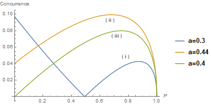
Figure 1: The variation of the concurrence with $P$ for three different input states with state parameters $a=0.3$, $0.44$ and $0.4$ are represented by the blue, yellow and green plots. For these three input states, other state parameters are $c=0.2$ and $d=0.4$. The blue plot represents scenario (i) which first shows entanglement sudden death and then a rebirth of entanglement and finally asymptotically decays to zero. The yellow plot represent scenario (ii) which first shows creation of entanglement and finally asymptotically decays to zero. The green plot represent scenario (iii) where the concurrence first becomes nonzero and gradually increases and finally asymptotically decreases to zero.

Let us now examine the scenario (i) in detail with an example. Consider an intraparticle entangled state with state parameter $a=0.3$, $c=0.4$ and $d=0.6$. Here $ad=0.18$, $bc=0.25$ and $ad<bc$ is satisfied. For this input state, the variation of the quantities $\alpha$, $\sqrt{\beta}$ and $(1-P)\sqrt{\beta}$ with channel parameter $P$ are shown in Fig. 2. In Fig. 2 we notice that $\alpha$ increases with channel parameter $P$ and attains its maximum value $0.08$ at $P=0.5$. After that it gradually decreases and becomes zero at $P=1$. At $P=0$, $\alpha=\sqrt{\beta}$. With the increase of $P$, $\sqrt{\beta}$ first increases and reaches its maximum value $0.02$ at $P=0.124$ and then decreases to $0$ at $P=1-\frac{a^{2}d^{2}}{b^{2}c^{2}}=0.48$. After that it again increases and attains its maximum value $0.014$ at $P=0.8$ and finally decreases to $0$ at $P=1$. The behaviour of $(1-P)\sqrt{\beta}$ is similar to that of $\sqrt{\beta}$. With the increase of $P$, $(1-P)\sqrt{\beta}$ first increases and reaches its maximum value $0.017$ at $P=0.086$ and then decreases to $0$ at $P=1-\frac{a^{2}d^{2}}{b^{2}c^{2}}=0.48$. After that it again increases and attains its maximum value $0.004$ at $P=0.67$ and then finally decreases to $0$ at $P=1$.

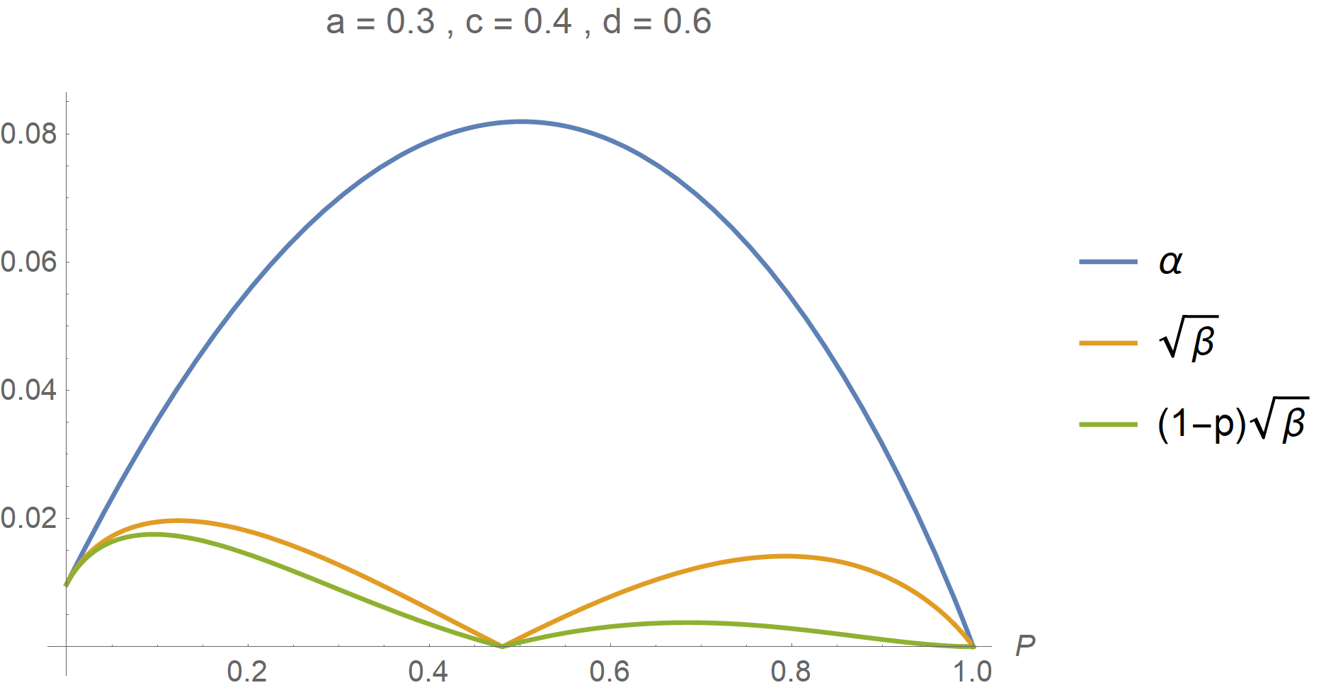
Figure 2: In this figure the quantities $\alpha$, $\sqrt{\beta}$ and $(1-P)\sqrt{\beta}$ are plotted for input state parameters $a=0.3$, $c=0.4$ and $d=0.6$ and $P$ is varied from $0$ to $1$.

The behaviour of $\lambda_{1}$ and $\lambda_{2}$ as a function of the channel parameter $P$ is shown in the Fig. 3. Recall the behaviour of $\alpha$ and $(1-P)\sqrt{\beta}$: Since $\lambda_{1}=\alpha+(1-P)\sqrt{\beta}$ and $\lambda_{2}=\alpha-(1-P)\sqrt{\beta}$, the behaviour of $\lambda_{1}$ and $\lambda_{2}$ can be easily explained from the behaviour of $\alpha$ and $(1-P)\sqrt{\beta}$. In Fig. 3, we observe that for $P<1-\frac{a^{2}d^{2}}{b^{2}c^{2}}=0.48$ and $P>1-\frac{a^{2}d^{2}}{b^{2}c^{2}}=0.48$, $\lambda_{1}$ is always greater than $\lambda_{2}$. At the point $P=1-\frac{a^{2}d^{2}}{b^{2}c^{2}}=0.48$, $\lambda_{1}=\lambda_{2}$.

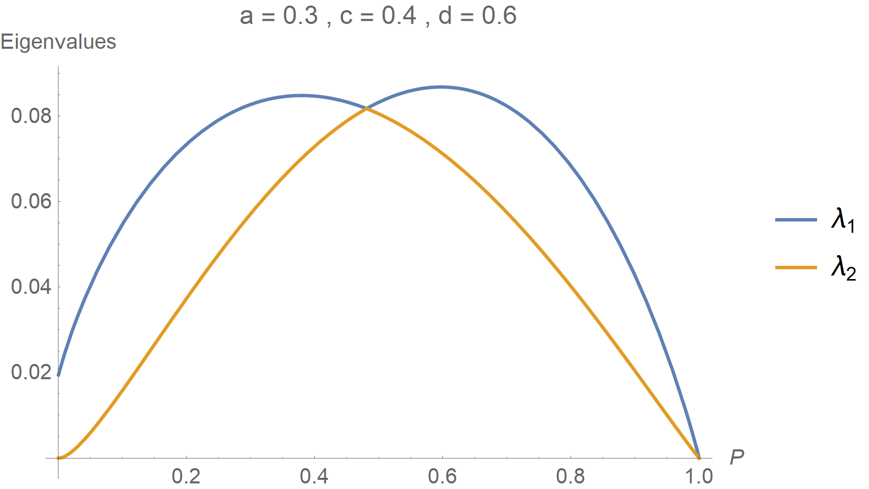
Figure 3: In this figure two eigenvalues $\lambda_{1}$ and $\lambda_{2}$ are plotted for input state parameters $a=0.3$, $c=0.4$ and $d=0.6$ and $P$ is varied from $0$ to $1$.

Since the concurrence $C=\sqrt{\lambda_{1}}-\sqrt{\lambda_{2}}$, in Fig. 4 we plot $\sqrt{\lambda_{1}}$, $\sqrt{\lambda_{2}}$ and the concurrence as a function of $P$. The behaviour of $\sqrt{\lambda_{1}}$, $\sqrt{\lambda_{2}}$ is similar to the behaviour of $\lambda_{1}$ and $\lambda_{2}$. In Fig. 4 we observe that for $P<1-\frac{a^{2}d^{2}}{b^{2}c^{2}}=0.48$ and $P>1-\frac{a^{2}d^{2}}{b^{2}c^{2}}=0.48$, $\sqrt{\lambda_{1}}$ is always greater than $\sqrt{\lambda_{2}}$ and the concurrence is nonzero. At the point $P=1-\frac{a^{2}d^{2}}{b^{2}c^{2}}=0.48$, $\sqrt{\lambda_{1}}=\sqrt{\lambda_{2}}$ and the concurrence is zero.

After the point $P=1-\frac{a^{2}d^{2}}{b^{2}c^{2}}=0.48$, since the concurrence again becomes nonzero we call this is the rebirth of intraparticle entanglement. Thus, there is a direct correlation between the rebirth of intraparticle entanglement and the behaviour the two eigenvalues $\lambda_{1}$ and $\lambda_{2}$.

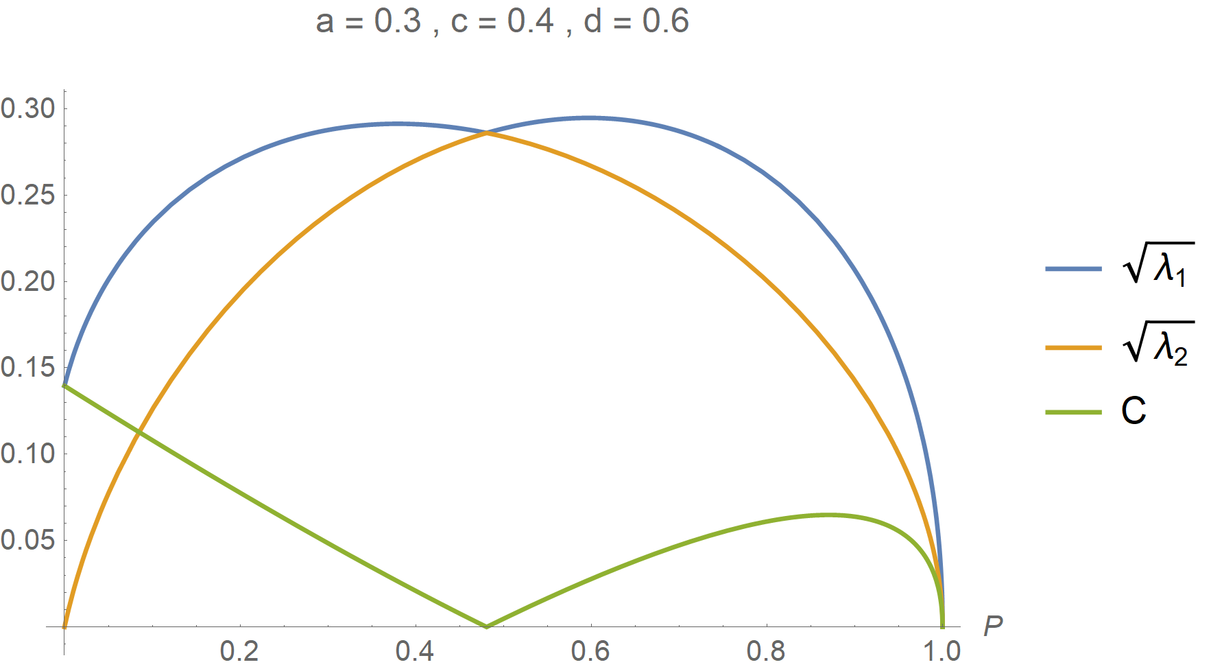
Figure 4: In this figure $\sqrt{\lambda_{1}}$, $\sqrt{\lambda_{2}}$ and the concurrence $C$ are plotted for input state parameters $a=0.3$, $c=0.4$ and $d=0.6$ and $P$ is varied from $0$ to $1$.

Scenario (ii) and scenario (iii) can also be explained in a similar way.

In the example discussed above, note that all input state parameters take on positive values. As our observations are dependent on the subtle interplay between channel and input state parameters, we also investigate cases where the input state parameters are not all positive. We indeed get new findings if we allow all those states where input state parameters $a$, $b$, $c$, and $d$ can take values from $-1$ to $1$. For states where all of the input state parameters take on the same sign (all being either positive or negative), or cases where even number of input state parameters are positive and others are negative, we observe entanglement sudden death, rebirth of entanglement as well as creation of entanglement. On the other hand, in those states where an odd number of input state parameters are positive and other parameters are negative, we only observe the asymptotic decay of entanglement and no entanglement sudden death or rebirth of entanglement is observed.

Next, for the sake of comparison, we consider the decoherence of an inter-particle entangled state $|\psi\rangle_{in}$ under the amplitude damping channel. Since particles $A$ and $B$ are spatially separated, the environment acts on each particle locally and the relevant Kraus operators representing a local amplitude damping channel are Almeida2008

$$M_{0}=\begin{pmatrix}1&0\\ 0&\sqrt{1-P}\end{pmatrix}~{}~{}~{}~{},~{}~{}~{}~{}M_{1}=\begin{pmatrix}0&\sqrt{P}\\ 0&0\end{pmatrix}$$

Here, we assume that two local amplitude damping channels are identical. After passing through the amplitude damping channel, the concurrence of the output state becomes

$$C=max\Big{[}0,\sqrt{\alpha+\beta}-\sqrt{\alpha-\beta}-2d^{2}P(1-P)\Big{]}$$ (7)

where

$$\alpha = 2(ad-bc)^{2}(1-P)^{2}+d^{4}P^{2}(1-P)^{2},$$

$$\beta = 2(ad-bc)^{2}(1-P)^{2}\sqrt{1-\frac{d^{4}}{(ad-bc)^{2}}P^{2}}$$ (8)

Using the constraint relation $b^{2}=1-a^{2}-c^{2}-d^{2}$, one can express the concurrence as a function of $a$, $c$, $d$ and $P$. To compare its dynamics with that of intraparticle entangled state, we consider $a=c=\frac{1}{4}$. Fig. 5 shows the variation of the concurrence with $P$ for different values of $d$. From the Fig. 5 we see that for all non zero values of $d$, Concurrence becomes zero for $P<1$. For $d=0$, the concurrence drops linearly to zero at $P=1$. So interparticle entanglement does not show any revival of entanglement as well as initial increase of entanglement for any input pure state under the amplitude damping channel. For nonzero values of $d$, Fig. 5 shows that one can always get ESD. But no rebirth of entanglement occurs after ESD.

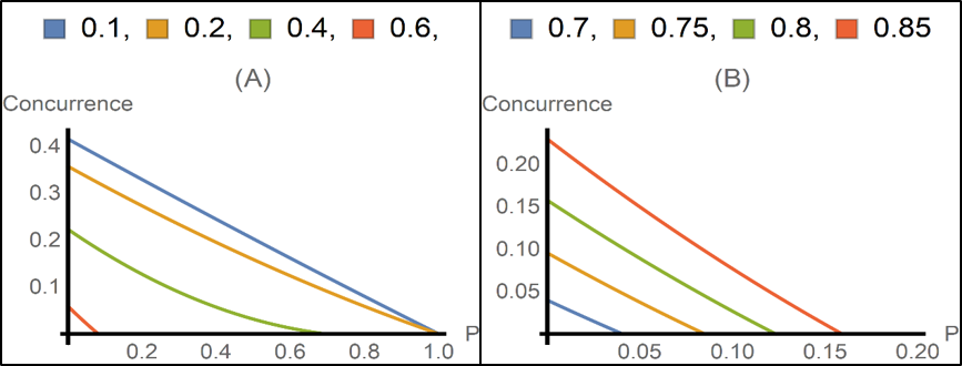
Figure 5: In the Fig. 5(A), 5(B) the Concurrence is plotted as a function of $P$ for $a=c=\frac{1}{4}$ and two different ranges of $d$, $d<\frac{\sqrt{7}}{4}=0.66$ and $\frac{\sqrt{7}}{4}=0.66\leq d$ respectively. At $d=\frac{\sqrt{7}}{4}=0.66$, input state is a separable state and we do not observe any effect of the channel on the entanglement.

Next, we compare the decoherence of several intraparticle entangled states with interparticle entangled states for fixed input state parameters $a=c=\frac{1}{4}$ and different $d$ parameter values as shown in the Fig. 6. In the state parameter range $d<\frac{\sqrt{7}}{4}=0.66$ intraparticle entanglement shows ESD as well as rebirth of entanglement which finally decays to $0$ at $P=1$, while interparticle entanglement shows ESD but no rebirth of entanglement occurs as shown in the Fig. 6(A). ESD for interparticle entangled state occurs earlier compared to intraparticle entangled state. In the range $0.66<d\leq 0.83$, intraparticle entanglement initially increased and then finally decreased to $0$ at $P=1$ and interparticle entanglement shows ESD as shown in the Fig. 6(B). In the range $d>0.83$ intraparticle entanglement decreased to $0$ at $P=1$, while interparticle entanglement shows ESD as shown in the Fig. 6(C). Here, notably, for the value $d=0.66$, creation of intraparticle entanglement occurs, which finally decays to $0$ at $P=1$ while the channel has no effect on the bipartite interparticle state. Thus, intraparticle entanglement decays more slowly than interparticle entanglement for all ranges of input state parameters.

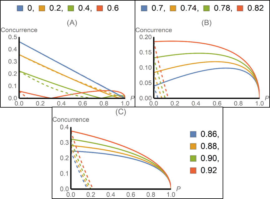
Figure 6: In the Fig. 6(A), 6(B) and 6(C) Concurrence for intraparticle entangled states and interparticle entangled states are plotted as a function of $P$ for three different ranges of $d$, $0<d<\frac{\sqrt{7}}{4}=0.66$, $\frac{\sqrt{7}}{4}=0.66\leq d\leq 0.83$ and $0.83\leq d\leq 0.93$ respectively.In the figure, solid curves represent concurrence for intraparticle entangled state while the dashed curves represent concurrence for interparticle entangled state. From the curve it is clear that only intraparticle entanglement showing rebirth and creation of entanglement.

In BBellomo , the authors have shown a revival of interparticle entanglement under the non-Markovian dissipative Amplitude damping channel where the ADC parameter takes a special form

$$P=e^{-\Gamma t}\Bigg{(}\cos(\frac{dt}{2})+\frac{\Gamma}{d}\sin(\frac{dt}{2})\Bigg{)}^{2}$$ (9)

where $d=\sqrt{2\gamma\Gamma-\Gamma^{2}}$ and $t$ is the time parameter. In order to get revival of interparticle entanglement one needs the specific model of ADC channel parameter, while one can get revival of intraparticle entanglement without considering any specific model of ADC channel parameter. Thus, the revival of intraparticle entanglement under the amplitude damping channel is model independent whereas, one can observe revival of interparticle entanglement only under specific model dependent forms for the amplitude damping channel.

III Other damping channels

We have investigated the effect of the phase damping and the depolarizing channels separately on a pure intraparticle entangled state $|\psi\rangle_{in}$. We do not observe any rebirth of intraparticle entanglement after entanglement sudden death or creation of intraparticle entanglement. We have also calculated the decoherence of a pure interparticle entangled state under the phase damping and depolarizing channels. We have compared this result with the decoherence of the intraparticle entangled state and have observed that the decay of interparticle entanglement is much faster than the decay of intraparticle entanglement. The detailed calculation for these cases has been included in the Appendix.

IV Concluding Remarks

In conclusion, we have demonstrated the unexpected phenomenon of entanglement generation of intraparticle entanglement under the amplitude damping channel starting from a separable state. This arises due to the interplay of channel and state parameters, not observed in the interparticle scenario. This subtle interplay also leads to entanglement sudden death and its regeneration for partially entangled input states. For maximally entangled states, we only observe asymptotic decay in both the intraparticle and interpartcle entanglement scenario. This shows the relevance of the amplitude damping channel for partially entangled and separable input states, and can be used to distinguish inter and intraparticle entanglement. It is worth emphasising that this behaviour is not seen for interparticle entanglement without consideration of non-Markovian noise which happens because of information backflow. In comparison, the phase and depolarizing channels only show the general robustness of intraparticle entanglement as compared to interparticle entanglement.

Appendix A Phase damping Channel

When a quantum system loses quantum information without losing its energy during the interaction with the environment, the process is known as phase damping. During phase damping, relative phase among the eigenstates of the system is lost. The Kraus operators for the phase damping channel are :-

$$M_{0} = \sqrt{1-P}\sum_{j=0}^{d-1=3}|j\rangle\langle j|,$$

$$M_{i+1} = \sqrt{P}|i\rangle\langle i|,(i=0,1,2,3)$$ (10)

After evolution of the intraparticle entangled state $|\psi\rangle_{in}$ through a phase damping channel, the final state becomes

$$\rho_{out}=\begin{pmatrix}a^{2}&abq&acq&adq\\ abq&b^{2}&bcq&bdq\\ acq&bcq&c^{2}&cdq\\ adq&bdq&cdq&d^{2}\end{pmatrix}$$ (11)

where $q=1-P$. Next we calculate the matrix $R$ [Eq. (3)] and find out all four eigenvalues of this matrix. They are

$$\lambda_{1} = \frac{1}{2}\Big{[}\alpha+(ad-bc)(2-P)\sqrt{\beta}\Big{]}~{}~{},$$

$$\lambda_{2} = \frac{1}{2}\Big{[}\alpha-(ad-bc)(2-P)\sqrt{\beta}\Big{]}~{}~{},$$

$$\lambda_{3} = a^{2}d^{2}P^{2}~{}~{},$$

$$\lambda_{4} = b^{2}c^{2}P^{2}$$ (12)

where

$$\alpha = (ad-bc)^{2}(2-P)^{2}+2abcdP(4-3P)$$

$$\beta = (ad-bc)^{2}(2-P)^{2}+4abcdP(4-3P)$$ (13)

Let us first consider the case where $a$, $b$, $c$ and $d$ are all positive numbers. In that situation $\alpha$ and $\beta$ are both positive. Here we consider two different cases.

Case -(1) $ad>bc$. In this case $\lambda_{1}$ is the largest eigenvalue. Let us consider the situation where $P=0$, i.e. with no effect of phase damping noise. Then the eigenvalues become

$$\lambda_{1}=4(ad-bc)^{2}~{}~{},~{}~{}\lambda_{2}=\lambda_{3}=\lambda_{4}=0$$

So, only $\lambda_{1}$ contributes to the expression of the concurrence , i.e., $C=\sqrt{\lambda_{1}}=2(ad-bc)$, while other three eigenvalues have no contribution to the concurrence. If we increase the channel parameter $P$ gradually we observe that the eigenvalue $\lambda_{1}$ remains the largest eigenvalue with the increase of $P$ while the other three eigenvalues first become nonzero and then increase gradually. At $P=1$,

$$\lambda_{1}=a^{2}d^{2}=\lambda_{3}~{}~{},~{}~{}\lambda_{2}=b^{2}c^{2}=\lambda_{4}$$

As a result the concurrence $C=0$ at $P=1$. Let us now find the value of the channel parameter $P$ where the concurrence becomes zero. When $C=0$, the following condition is satisfied:

$$\sqrt{\lambda_{1}}=\sqrt{\lambda_{2}}+\sqrt{\lambda_{3}}+\sqrt{\lambda_{4}}$$

Substituting expressions of all $\lambda_{i}$ in the above equation and solving it for $P$ we get following acceptable solution of $P$:

$$P = \frac{ad-bc}{ad}$$

Depending on the values of the input state parameters, we will get ESD at specific value of $P$.

Case - (2) $ad<bc$. In this case, $\lambda_{2}$ is the largest eigenvalue. At $P=0$,

$$\lambda_{2}=4(ad-bc)^{2}~{}~{},~{}~{}\lambda_{1}=\lambda_{3}=\lambda_{4}=0$$

So, only $\lambda_{2}$ contributes to the expression of the concurrence , i.e., $C=\sqrt{\lambda_{2}}=2(ad-bc)$, while other three eigenvalues have no contribution to the concurrence. If we increase the channel parameter $P$ gradually we observe that the eigenvalue $\lambda_{2}$ remains the largest eigenvalue with the increase of $P$ while the other three eigenvalues first become nonzero and then increases gradually. At $P=1$,

$$\lambda_{1}=a^{2}d^{2}=\lambda_{3}~{}~{},~{}~{}\lambda_{2}=b^{2}c^{2}=\lambda_{4}$$

and the concurrence is zero. At the point when $C=0$,

$$\sqrt{\lambda_{2}}=\sqrt{\lambda_{1}}+\sqrt{\lambda_{3}}+\sqrt{\lambda_{4}}$$

Substituting expressions of all $\lambda_{i}$ in the above equation and solving it for $P$ we get the following acceptable solution of $P$:

$$P = \frac{bc-ad}{bc}$$

In this case also depending on the input state parameter, we will get ESD at a specific value of $P$.

From this analysis we observe that there is no single eigenvalue which is largest for all input state parameters $a$, $b$, $c$ and $d$. If $ad>bc$, $\lambda_{1}$ is the largest eigenvalue and if $ad<bc$, $\lambda_{2}$ is the largest eigenvalue. In both cases a commonality is that when one eigenvalue becomes largest, it remains largest for the entire range of $P$. Let us denote the largest eigenvalue as $\lambda_{max}$ and the sum of square root of remaining three eigenvalues as $\lambda_{rest}$. When $ad>bc$, $\lambda_{1}$ is the largest eigenvalue and $\lambda_{max}=\lambda_{1}$ and $\sqrt{\lambda_{2}}+\sqrt{\lambda_{3}}+\sqrt{\lambda_{4}}=\lambda_{rest}$. On the other hand, When $ad<bc$, $\lambda_{2}$ is the largest eigenvalue and $\lambda_{max}=\lambda_{2}$ and $\sqrt{\lambda_{1}}+\sqrt{\lambda_{3}}+\sqrt{\lambda_{4}}=\lambda_{rest}$. There is a physical value of the channel parameter $P$ where we observe ESD. Below the ESD point where $\sqrt{\lambda_{max}}>\lambda_{rest}$ we get nonzero Concurrence and above the ESD point where $\sqrt{\lambda_{max}}<\lambda_{rest}$ we get zero Concurrence. If we observe the condition $\sqrt{\lambda_{max}}>\lambda_{rest}$ after the ESD point, we can say that rebirth of intraparticle entanglement occurs. But, for the phase damping channel this does not happen.

Next consider decoherence of an inter-particle entangled state $|\psi\rangle_{in}$ under the phase damping channel. The effect of noise due to phase damping channel can be described by the following three Kraus operators preskill98 ,

$$M_{0}=\sqrt{q}\begin{pmatrix}1&0\\ 0&1\end{pmatrix},M_{1}=\sqrt{P}\begin{pmatrix}1&0\\ 0&0\end{pmatrix},M_{2}=\sqrt{P}\begin{pmatrix}0&0\\ 0&1\end{pmatrix}$$

After evolution of $|\psi\rangle_{in}$ through the phase damping channel, the final state becomes

$$\rho_{out}=\begin{pmatrix}a^{2}&abq&acq&adq^{2}\\ abq&b^{2}&bcq^{2}&bdq\\ acq&bcq^{2}&c^{2}&cdq\\ adq^{2}&bdq&cdq&d^{2}\end{pmatrix}$$ (14)

where $q=1-P$. To investigate the nature of decoherence of an interparticle entangled state, we consider input state parameters $a=c=\frac{1}{4}$. Fig. 7 shows the variation of the concurrence with $P$ for different values of input state parameter $d$. For $d=0$, the concurrence drops to zero when $P=1$. For all non zero values of $d$, the concurrence becomes zero for value of $P<1$.

Fig. 8 shows decoherence of both intraparticle and interparticle entanglement as a function of the channel parameter $P$. Here the solid and dashed graphs represent the concurrence of intraparticle entangled state and interparticle entangled state respectively. From the Fig. 8 one can easily say that interparticle entanglement decays more rapidly compared to intraparticle entanglement.

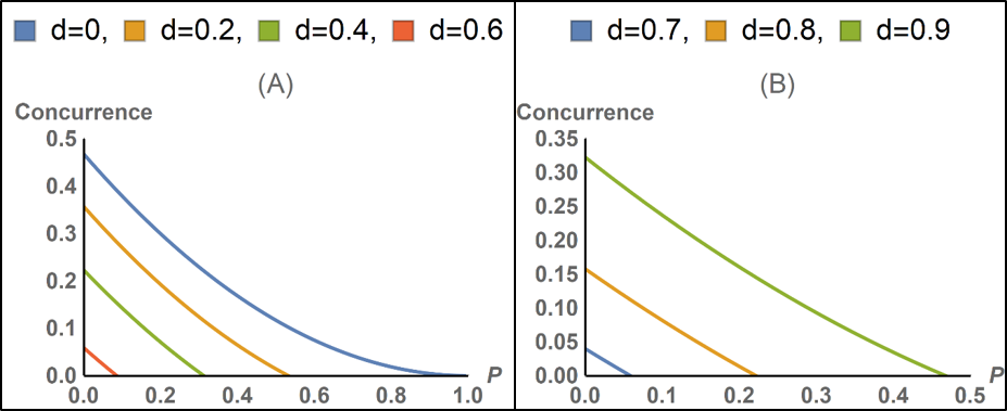
Figure 7: Evolution of the concurrence of pure interparticle entangled states with channel parameter $P$ for $a=c=\frac{1}{4}$ and different values of $d$ under the phase damping channel is shown in this figure. In the Fig. 7(A) and Fig. 7(B), $d$ takes the value $0,0.2,0.4,0.6$ and $0.7,0.8,0.9$ respectively. This shows that the concurrence decays non-linearly with the increase of $P$. For $d=0$, the concurrence drops to zero when $P=1$. For all non zero values of $d$, the concurrence becomes zero for value of $P<1$.

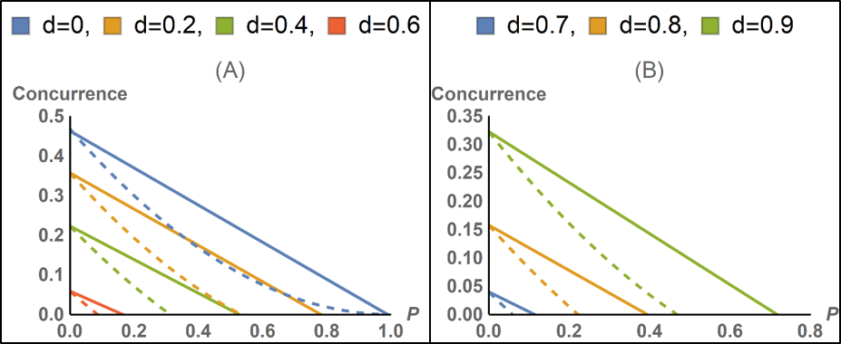
Figure 8: Evolution of the concurrence of pure intraparticle entangled states and pure interparticle entangled states with channel parameter $P$ for $a=c=\frac{1}{4}$ and different values of $d$ under the effect of the phase damping channel is shown in this figure. In the Fig. 8(A) and Fig. 8(B), d takes the value $0,0.2,0.4,0.6$ and $0.7,0.8,0.9$ respectively. Both the Fig. 8(A) and Fig. 8(B) show that interparticle entanglement decays more rapidly compared to intraparticle entanglement under the effect of the phase damping channel.

Appendix B Depolarising channel

Under the action of a depolarising channel, a d-level quantum system becomes a maximally mixed state $\mathcal{I}/d$ with finite probability $P$. Kraus operators corresponding to this channel are PooladImany ; PGokhale

$$M_{00} = \sqrt{1-\frac{d^{2}-1}{d^{2}}P}~{}\hat{U}_{00}=\sqrt{1-\frac{15}{16}P}~{}~{}\hat{U}_{00},$$

$$M_{ij} = \frac{\sqrt{p}}{4}\hat{U}_{ij}~{},~{}0\leq i,j\leq 3~{}~{}and~{}~{}(i,j)\neq(0,0)$$

where $\hat{U}_{ij}$ are the Weyl operators. In a $d$ dimensional Hilbert space, the Weyl operators $\hat{U}_{mn}$ are a set of $d^{2}$ operators defined as Bertlmann2008 ; AlejandroFonseca

$$\hat{U}_{mn}=\sum_{j=0}^{d-1}e^{\frac{2\pi i}{d}jm}|j\rangle\langle j+n~{}~{}mod~{}~{}d|$$ (15)

Weyl operators are unitary operators and form an orthonormal basis of the Hilbert space, known as the Weyl operator basis. In our present scenario $d=4$. So

$$\hat{U}_{mn} = \sum_{j=0}^{3}e^{\frac{2\pi i}{d}jm}|j\rangle\langle j+n~{}~{}mod~{}~{}4|$$ (16)

$$= |0\rangle\langle n|+e^{i\frac{m\pi}{2}}|1\rangle\langle n+1|+e^{im\pi}|2\rangle\langle n+2|$$

$$+ e^{i\frac{3m\pi}{2}}|3\rangle\langle n+3|$$

There are 16 Weyl operators in a $4$ dimensional Hilbert space.

Under the action of a depolarising channel, a d-level quantum system becomes a maximally mixed state $\mathcal{I}/d$ with finite probability $P$. After the evolution of $|\psi\rangle_{in}$ through a depolarising channel, the final state becomes

$$\rho_{out}=\begin{pmatrix}a^{2}q+\frac{P}{4}&abq&acq&adq\\ abq&b^{2}q+\frac{P}{4}&bcq&bdq\\ acq&bcq&c^{2}q+\frac{P}{4}&cdq\\ adq&bdq&cdq&d^{2}q+\frac{P}{4}\end{pmatrix}$$ (17)

where $q=1-P$. Next we calculate the matrix $R$ [Eq. (3)] and find out all four eigenvalues of this matrix. They are

$$\lambda_{1} = \alpha+\beta~{},~{}\lambda_{2}=\alpha-\beta~{},~{}\lambda_{3}=\lambda_{4}=\frac{P^{2}}{16}$$ (18)

where

$$\alpha = 2(ad-bc)^{2}(1-P)^{2}+\frac{P}{4}(1-\frac{3P}{4}),$$

$$\beta = 2|(ad-bc)|(1-P)\sqrt{(ad-bc)^{2}(1-P)^{2}+\frac{P}{4}(1-\frac{3P}{4})}$$

Among four eigenvalues, $\lambda_{3}$ and $\lambda_{4}$ are input state parameter independent. They depend only on channel parameter $P$. At $P=0$, $\lambda_{3}=\lambda_{4}=0$. With the increase of $P$ they increase linearly and attain their maximum value $1/16$ at $P=1$. For $a$, $b$, $c$ and $d$ taking positive and negative values, $\alpha$ and $\beta$ are always positive. So, the eigenvalue $\lambda_{1}$ is always greater than $\lambda_{2}$. At $P=0$, no effect of depolarizing noise is there. At that point $\alpha=\beta=2(ad-bc)^{2}$ and $\lambda_{1}=4(ad-bc)^{2}$, $\lambda_{2}=0$. So, only $\lambda_{1}$ contributes to the expression of the concurrence , i.e., $C=\sqrt{\lambda_{1}}=2(ad-bc)$, while other three eigenvalues have no contribution to the concurrence. If we increase the channel parameter $P$ gradually we observe that the eigenvalue $\lambda_{1}$ remains the largest eigenvalue with the increase of $P$ while the other three eigenvalues first become nonzero and then increase gradually. At the point when $C=0$, the following condition is satisfied:

$$\sqrt{\lambda_{1}}=\sqrt{\lambda_{2}}+\sqrt{\lambda_{3}}+\sqrt{\lambda_{4}}$$

Substituting expressions of all $\lambda_{i}$ in the above equation and solving it for $P$ we get following acceptable solution of $P$:

$$P=\frac{4|(ad-bc)|}{1+4|(ad-bc)|}$$ (20)

Since $\frac{4|(ad-bc)|}{1+4|(ad-bc)|}<1$, we always get entanglement sudden death in this case. $P$ becomes maximum when one start from a maximally entangled pure Bell state for which $P=\frac{2}{3}$ when ESD occurs. For nonmaximally entangled pure state $P<\frac{2}{3}$.

From the above analysis we observe that the eigenvalue $\lambda_{1}$ is always larger than any other three eigenvalues for all possible input state parameters and channel parameter. There is a physical value of the channel parameter $P$ where $\sqrt{\lambda_{1}}=\sqrt{\lambda_{2}}+\sqrt{\lambda_{3}}+\sqrt{\lambda_{4}}$ and we observe ESD. Below the ESD point where $\sqrt{\lambda_{1}}>\sqrt{\lambda_{2}}+\sqrt{\lambda_{3}}+\sqrt{\lambda_{4}}$ we get nonzero Concurrence and above the ESD point where $\sqrt{\lambda_{1}}<\sqrt{\lambda_{2}}+\sqrt{\lambda_{3}}+\sqrt{\lambda_{4}}$ we get zero Concurrence. If we observe the condition $\sqrt{\lambda_{1}}>\sqrt{\lambda_{2}}+\sqrt{\lambda_{3}}+\sqrt{\lambda_{4}}$ after the ESD point, we can say that rebirth of intraparticle entanglement occurs. But, this does not happen for the depolarizing channel.

Next consider an interparticle entangled state under a depolarising channel. We consider that the channel parameters for particle $A$ and $B$ are same and equal to $P$. After evolution of $|\psi\rangle_{in}$ through a depolarising channel, the final state concurrence becomes a function of $a$, $c$, $d$ and $P$ where we replace $b$ using the relation $b^{2}=1-a^{2}-c^{2}-d^{2}$. To investigate the decay of interparticle entanglement under the depolarizing channel, consider specific values of $a$ and $c$ as $a=c=\frac{1}{4}$. In this case, decay of the concurrence with channel parameter $P$, for different values of $D$ is shown in the fig. 9. From Fig. 9 one can say that the concurrence decays linearly with the increase of channel parameter $P$. For all allowed values of $D$, the concurrence become zero when $P<1$. So, for all values of $D$, ESD occurs. Higher the initial Concurrence, longer it takes to decay out under the effect of this noise.

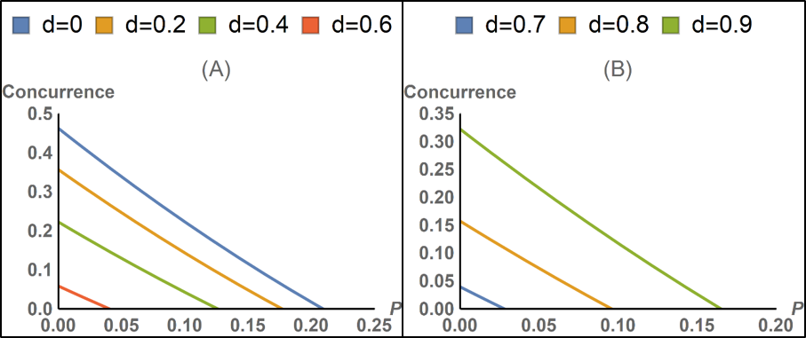
Figure 9: Evolution of the concurrence of pure interparticle entangled states with channel parameter $P$ for $a=c=\frac{1}{4}$ and difference values of $d$ under the effect of the depolarising channel is shown in this figure. In the Fig. 9(A) and Fig. 9(B), d takes the value $0,0.2,0.4,0.6$ and $0.7,0.8,0.9$ respectively. This figure shows that the concurrence decays linearly with the increase of $P$. For all possible values of $d$, ESD occur.

Next, we compare the decoherence between an intraparticle entangled state and an interparticle entangled state under depolarizing channel. So, we consider an intraparticle entangled state and an interparticle entangled state with same initial Concurrence value and check the nature of the decay of both types of entanglement under the depolarizing channel. Fig. 10 shows the decoherence of both types of entanglement. In the fig. 10 solid curves represent the concurrence of intraparticle entangled states while the dashed curves represent the concurrence of interparticle entangled states. From the Fig. 10 one can easily say that interparticle entanglement decays more rapidly compared to the intraparticle entanglement. So intraparticle entanglement is more robust compared to the interparticle entanglement under the effect of the depolarizing channel.

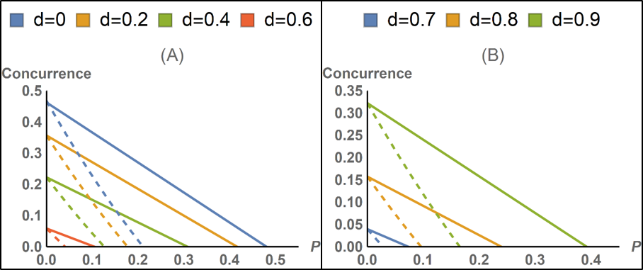
Figure 10: Evolution of the concurrence of pure intraparticle entangled states and pure interparticle entangled states with channel parameter $P$ for $a=c=\frac{1}{4}$ and difference values of $d$ under the effect of the depolarising channel is shown in this figure. In the Fig. 10(A) and Fig. 10(B), d takes the value $0,0.2,0.4,0.6$ and $0.7,0.8,0.9$ respectively. Both the fig. 10(A) and Fig. 10(B) show that interparticle entanglement decays much more rapidly compared to the intraparticle entanglement under the effect of the depolarizing channel.

References

- (1) J. S. Bell , Physics 1, 195 (1964).
- (2) J. F. Clauser, M. A. Horne, A. Shimony, and R. A. Holt, Phys. Rev. Lett. 23, 880 (1969).
- (3) S. Basu, S. Bandyopadhyay, G. Kar, D. Home, Phys. Lett. A 279, 281 (2001).
- (4) S. Kochen, E. Specker, J. Math. Mech. 17, 59 (1967).
- (5) M. Michler, H. Weinfurter, M. Żukowski, Phys. Rev. Lett. 84, 5457 (2000).
- (6) B. R. Gadway, E J Galvez, F. De. Zela, J. Phys. B: At. Mol. Opt. Phys. 42, 015503 (2009).
- (7) A. Mair, A. Vaziri, G. Weihs, A. Zeilinger, Nature 412, 313 (2001).
- (8) J. Barreiro, N. K. Lankford, N. A. Peters, P. G. Kwiat, Phys. Rev. Lett. 95, 260501 (2005).
- (9) Y. Hasegawa, R. Loidl, G. Badurek, M. Baron, H. Rauch, Nature 425, 45 (2003).
- (10) J. Shen, S. J. Kuhn, R. M. Dalgliesh, V. O. de Haan, N. Geerits, A. A. M. Irfan, F. Li, S. Lu, S. R. Parnell, J. Plomp, A. A. van Well, A. Washington, D. V. Baxter, G. Ortiz, W. M. Snow, and R. Pynn, Nat. Commun. 11, 930 (2020).
- (11) Y. Sun, Q.-Y. Wen, Z. Yuan, Opt. Commun. 284, 527 (2011).
- (12) S. Adhikari, D. Home, A. S. Majumdar, A. K. Pan, Akshata Shenoy H, · R. Srikanth, Quantum Inf Process 14, 1451 (2015).
- (13) J. Heo, C.-H. Hong, J.-I. Lim, H.-J. Yang, Chin. Phys. B 24, 050304 (2015).
- (14) T. Pramanik, D. Home, S. Adhikari, A. Pan, Phys. Lett. A 374, 1121 (2010).
- (15) J. Heo, C.-H. Hong, J.-I. Lim, H.-J. Yang, Int. J. Theor. Phys. 54, 2261 (2015).
- (16) S. Adhikari, A. Majumdar, D. Home, A. Pan, Eur. Phys. Lett. 89, 10005 (2010).
- (17) T. Yu, J. Eberly, Science 323, 598 (2009).
- (18) M. P. Almeida, E. De MELO, M. Hor-Meyll, A. Salles, S. P. Walborn, P. H. Souto Ribeiro, and L. Davidovich, Science 316, 579 (2007).
- (19) A. Salles, F. de Melo, M. P. Almeida, M. Hor-Meyll, S. P. Walborn, P. H. Souto Ribeiro, and L. Davidovich, Phys. Rev. A 78, 022322 (2008).
- (20) William K. Wootters, Phys. Rev. Lett. 80, 2245 (1998).
- (21) K. Kraus, States, Effects and Operations: Fundamental Notions of Quantum Theory Springer,Berlin, (1983).
- (22) B. Bellomo, R. Lo Franco, and G. Compagno, Phys. Rev. Lett. 99, 160502 (2007).
- (23) A Dutta, J Ryua, W Laskowskia, and M Zukowskia, Phys. Lett. A 380, 2191 (2016).
- (24) J. Preskill, “Quantum Information and Computation,” California Institute of Technology, 1998 (lecture notes).
- (25) P. Imany, J. A. Jaramillo-Villegas, M. S. Alshaykh, J. M. Lukens, O. D. Odele, A. J. Moore, D. E. Leaird, M. Qi, and A. M. Weiner, npj Quant. Info. 5,59 (2019).
- (26) P. Gokhale, J. M. Baker, C. Duckering, N. C. Brown, K. R. Brown, and F. T. Chong, Proceedings of the 46th International Symposium on Computer Architecture—ISCA ’19 (ACM, New York, 2019), pp. 554–566.
- (27) R. A. Bertlmann and P. Krammer, , J. Phys. A 41, 235303 (2008).
- (28) A Fonseca, Phys. Rev. A 100, 062311 (2019).