Methods used in nanostructure modeling

I. Camps
Laboratório de Modelagem Computacional - LaModel,
Instituto de Ciências Exatas - ICEx. Universidade Federal de Alfenas - UNIFAL-MG,
Alfenas, Minas Gerais, Brasil
HPQC Labs, Waterloo, Canada icamps@unifal-mg.edu.br

Abstract

How many times you need to change your method description because you were “accused” of plagiarism from text you already published? I will use this preprint to add all the methods I currently used in running the simulations for my research works. Then, I will cite it as needed.

Keywords: density functional theory, semiempirical, molecular dynamics, topology, tight binding.

1 Functionalizing Structures

In case of multiple functionalizations, populations of 10000 structures were generated for each system with the functional group (-OH, -COOH, etc.) added randomly to the surface sites. To choose a representative structure for each group/concentration, first, using OpenBabel software [1], the extended-connectivity fingerprints (ECFP) with bond diameter four (ECFP4) [2] was generated for each structure. ECFP4 was selected as it is currently one of the most used for similarity searching [3]. Then, the entropy of the binary fingerprint was calculated using the BiEntropy function [4]. This function is capable to identify order and disorder in binary strings. Finally, the most common structure was selected from the entropy distribution. Due to the volume of some groups (like -COOH) and the size of the base system used, it is only possible to add some percentage (5%, 10%, 15%, 20% and/or 25%) to cover the surface sites.

2 Metal nanoclusters

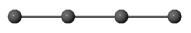
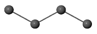
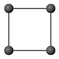
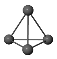
The metals considered here are in the form of isolated atoms and forming four–atom nanoclusters. In case of nanoclusters, were considered four different configurations: one dimensional linear chain (1DL, figure 1(a)), one dimensional zigzag chain (1DZ, figure 1(b)), two dimensional plane (2D, figure 1(c)) and three dimensional tetrahedron (3D, figure 1(d)). For notation completeness, the isolated atoms are labeled as 0D.

A script to generate the metal nanocluster is given in section S1.

3 SIESTA

All the studies presented in this work were done using the density functional theory (DFT) [5]. We used the SIESTA software [6] to optimize the geometry of the periodic structures and to calculate the electronic bands, density of states and binding energy. In this case, the generalized gradient approximation (GGA) was employed for the exchange-correlation potential using the PBE scheme [7]. The valence electrons were treated using a split-valence double- $\zeta$ basis set with polarization functions (DZP) [8] whereas the core electrons were represented using the norm-conserving Troullier-Martins pseudo potentials [9]. The accuracy of the results was guaranteed via convergence studies on the mesh-cutoff energy and the number of k-points. The energy convergence for the systems was obtained for a mesh-cutoff of $500$ Ry. For the number of k-points, the Brillouin zone was sampled in accordance with Monkhorst and Pack [10] with a $1\times 1\times 20$ k-point sampling set. All the properties were calculated on systems with fully relaxed atomic coordinates during geometry optimization until the Hellman-Feynman forces were below $0.03$ eVÅ^-1.

The atomic charge distribution was also determined from first principle calculations. In this work, we examine the charge density distribution using the Hirshfeld partition scheme [11] implemented in the SIESTA software. This partition scheme has proven to be highly insensitive to the choice of the basis set [11, 12].

4 Charges

One of the properties that can be calculated within the quantum mechanical approach is the partial atomic charge distribution. To accomplish this task, there are several methodologies like (i) Mulliken population analysis [13, 14, 15, 16], (ii) natural population analysis (NPA) [17], (iii) the Breneman-Wiberg (BW) model [18], (iv) Merz-Kollman-Singh (MKS) electrostatic potential derived charges [19, 20], (v) the Bader partition scheme [21, 22, 23, 24], (vi) the Voronoi partition scheme [25, 26] and (vii) the Hirshfeld partition scheme [11]. (vii) the CM5 scheme [27]. However, none of them is universally accepted as the “best” for computing partial atomic charges.

5 xTB

To perform the calculations, we used the semiempirical tight binding method, as implemented in the xTB program [28, 29]. Within the xTB program, there are implemented three different methods called GFNn-xTB, with $n=0,1,2$ . GFN0-xTB [30] is parameterized for all elements up to radon and includes only quantum mechanical contributions up to first–order, a classical electronegativity equilibration charge model and the atomic charge-dependent D4 dispersion correction to account for long range London correlation effects. GFN1-xTB uses similar second order with some terms up to third order approximations for the Hamiltonian and electrostatic energy as DFTB3 [31]. GFN2-xTB [32] uses a multipole electrostatic treatment up to quadrupole terms and the latest D4 dispersion model [33]

5.1 Docking

Using the automated Interaction Site Screening (aISS) [34], we generated different intermolecular geometries of the complexes and subjected them to further genetic optimization. The main idea of aISS is to find the global energy minimum (energetically lowest structure) of the largest interaction between two molecules. Firstly, a step is run to search for pockets in molecule A and then, a screening for $\pi-\pi$ –stacking interactions along different directions in three dimensions (3D). The next step is a search for global orientations of molecule B on an angular grid around molecule A. We used the interaction energy (xTB-IFF) [35] of each newly generated structure for ranking, and the genetic step was repeated ten times until the best complex was obtained. The best–ranked complexes were further subjected to structural optimization.

5.2 Geometry optimization

All geometry optimizations were performed using the GFN2–xTB method, which is an accurate self–consistent method that includes multipole electrostatics and density–dependent dispersion contributions [32]. Extreme optimization level was ensured, with a convergence energy of $5\times 10^{-8}$ E_h and gradient norm convergence of $5\times 10^{-5}$ E_h/a₀ (where a₀ is the Bohr radius).

6 Topological analysis

On topological analysis, one of the objectives is to determine the critical points. From the topological analysis point of view, critical points (CPs) are points where the gradient norm of the function value is zero. They are classified into four types depending on how the eigenvalues of Hessian matrix of real function are negative [21].

The CPs identified as $\bf(3,-3)$ occurs when three eigenvalues of the Hessian matrix are negative. They positions are nearly identical to atomic positions thus they are called nuclear critical point (NCP).

If two eigenvalues of the Hessian are negative (second–order saddle point), they are represented as $\bf(3,-1)$ . For electron density analysis, they generally appear between atom pairs, thus they are called bond critical point (BCP). The value of the electron density ( $\rho$ ) and the sign of its Laplacian ( $\nabla^{2}\rho$ ) can be related to the strength and type of the bonds formed [36].

If one eigenvalue of the Hessian is negative (first–order saddle point), they are represented as $\bf(3,+1)$ . For electron density analysis, they generally appear in the center of a ring system, thus they are called ring critical point (RCP).

Finally, if none of the eigenvalues are negative (local minimum) they are represented as $\bf(3,+3)$ . For electron density analysis, they generally appear in the center of a cage system, thus they are called cage critical point (CCP).

One way to classify the strength of bond (covalent or non-covalent) is to look at the electron density ( $\rho$ ) and the sign of its Laplacian ( $\nabla^{2}\rho$ ). Values of $\rho>0.20\,a.u.$ indicate a covalent bond whereas $\rho<0.10\,a.u.$ indicate a non-covalent bond. On the other hand, if $\nabla^{2}\rho<0$ , the bond can be classified as covalent and if $\nabla^{2}\rho>0$ can be classified as non covalent [36]. The ELF index is related to the electron movement confinement. Its value is in the range of $\left[0,1\right]$ . Large values mean that electrons are greatly localized indicating the presence of a covalent bond. The LOL index is another function for locating high localized regions [37]. Values of LOL index are also in the range of $\left[0,1\right]$ . Smaller (large) values usually appear in boundary (inner) regions.

7 Conclusion

We described here the main methods we currently use when running our computer simulations during our research.

References

[1] N. M. O'Boyle, M. Banck, C. A. James, C. Morley, T. Vandermeersch, G. R. Hutchison, Open Babel: An open chemical toolbox, J. Cheminf. 3 (2011). doi:10.1186/1758-2946-3-33.
[2] D. Rogers, M. Hahn, Extended-connectivity fingerprints, J. Chem. Inf. Model. 50 (2010) 742–754 (2010). doi:10.1021/ci100050t.
[3] G. Maggiora, M. Vogt, D. Stumpfe, J. Bajorath, Molecular similarity in medicinal chemistry, J. Med. Chem. 57 (2014) 3186–3204 (2014).
[4] G. Croll, BiEntropy, TriEntropy and primality, Entropy 22 (2020) 311 (2020). doi:10.3390/e22030311.
[5] R. M. Martin, Electronic structure: Basic theory and practical methods, Cambridge University Press, 2020 (2020). doi:10.1017/9781108555586.
[6] J. Soler, E. Artacho, J. Gale, A. García, J. Junquera, P. Ordejón, D. Sánchez-Portal, The SIESTA method for ab-initio order-N materials simulation, J. Phys. Condens. Matter 14 (2002) 2745–2779 (2002). doi:10.1088/0953-8984/14/11/302.
[7] J. P. Perdew, K. Burke, M. Ernzerhof, Generalized gradient approximation made simple, Phys. Rev. Lett. 77 (1996) 3865–3868 (1996). doi:10.1103/PhysRevLett.77.3865.
[8] E. Artacho, D. Sánchez-Portal, P. Ordejón, A. García, J. M. Soler, Linear-scaling ab-initio calculations for large and complex systems, Phys. Stat. Sol. (b) 215 (1999) 809–817 (1999). doi:10.1002/(SICI)1521-3951(199909)215:1<809::AID-PSSB809>3.0.CO;2-0.
[9] N. Troullier, J. L. Martins, Efficient pseudopotentials for plane-wave calculation, Phys. Rev. B 43 (1991) 1993–2006 (1991). doi:10.1103/PhysRevB.43.1993.
[10] H. J. Monkhorst, J. D. Pack, Special points for Brillouin-zone integrations, Phys. Rev. B 13 (1976) 5188–5192 (1976). doi:10.1103/PhysRevB.13.5188.
[11] F. L. Hirshfeld, Bonded-atom fragments for describing molecular charge densities, Theor. Chim. Acta 44 (1977) 129–138 (1977). doi:10.1007/BF00549096.
[12] F. Martin, H. Zipse, Charge distribution in the water molecule. A comparison of methods, J. Comput. Chem. 26 (2005) 97–105 (2005). doi:10.1002/jcc.20157.
[13] R. Mulliken, Electronic population analysis on LCAO–MO molecular wave functions. I, J. Chem. Phys. 23 (1955) 1833–1840 (1955).
[14] R. Mulliken, Electronic population analysis on LCAO–MO molecular wave functions. II. Overlap populations, bond orders, and covalent bond energies, J. Chem. Phys. 23 (1955) 1841–1846 (1955).
[15] R. Mulliken, Electronic population analysis on LCAO-MO molecular wave functions. III. Effects of hybridization on overlap and gross AO populations, J. Chem. Phys. 23 (1955) 2338–2342 (1955).
[16] R. Mulliken, Electronic population analysis on LCAO-MO molecular wave functions. IV. Bonding and antibonding in LCAO and valence-bond theories, J. Chem. Phys. 23 (1955) 2343–2346 (1955).
[17] A. E. Reed, R. B. Weinstock, F. Weinhold, Natural population analysis, J. Chem. Phys. 83 (1985) 735–746 (1985).
[18] C. M. Breneman, K. B. Wiberg, Determining atom-centered monopoles from molecular electrostatic potentials. The need for high sampling density in formamide conformational analysis, J. Comp. Chem. 11 (1990) 361–373 (1990).
[19] U. C. Singh, P. A. Kollman, An approach to computing electrostatic charges for molecules, J. Comp. Chem. 5 (1984) 129–145 (1984).
[20] B. H. Besler, K. M. Merz, P. A. Kollman, Atomic charges derived from semiempirical methods, J. Comp. Chem. 11 (1990) 431–439 (1990).
[21] Richard F. W. Bader, Atoms in Molecules: A Quantum Theory, Clarendon Press, 1994 (1994).
[22] G. Henkelman, A. Arnaldsson, H. Jónsson, A fast and robust algorithm for Bader decomposition of charge density, Comput. Mater. Sci. 36 (2006) 354–360 (2006).
[23] E. Sanville, S. Kenny, R. Smith, G. Henkelman, An improved grid-based algorithm for Bader charge allocation, J. Comp. Chem. 28 (2007) 899–908 (2007).
[24] W. Tang, E. Sanville, G. Henkelman, A grid-based Bader analysis algorithm without lattice bias, J. Phys.: Condens. Matter 21 (2009) 084204 (2009).
[25] F. M. Bickelhaup, N. J. R. van Eikema Hommes, C. F. Guerra, E. J. Baerends, The carbon–lithium electron pair bond in $(CH\_3Li)\_n$ (n = 1, 2, 4), Organometallics 15 (1996) 2923–2931 (1996).
[26] C. F. Guerra, J. W. Handgraaf, E. J. Baerends, F. M. Bickelhaupt, Voronoi deformation density (VDD) charges: Assessment of the Mulliken, Bader, Hirshfeld, Weinhold, and VDD methods for charge analysis, J. Comp. Chem. 25 (2004) 189–210 (2004).
[27] A. V. Marenich, S. V. Jerome, C. J. Cramer, D. G. Truhlar, Charge Model 5: an extension of Hirshfeld population analysis for the accurate description of molecular interactions in gaseous and condensed phases, Journal of Chemical Theory and Computation 8 (2012) 527–541 (2012). doi:10.1021/ct200866d.
[28] C. Bannwarth, E. Caldeweyher, S. Ehlert, A. Hansen, P. Pracht, J. Seibert, S. Spicher, S. Grimme, Extended tight-binding quantum chemistry methods, WIREs Comput. Mol. Sci. 11 (2020) e1493 (2020). doi:10.1002/wcms.1493.
[29] S. Grimme, C. Bannwarth, P. Shushkov, A robust and accurate tight-binding quantum chemical method for structures, vibrational frequencies, and noncovalent interactions of large molecular systems parametrized for all spd-block elements (Z=1–86), J. Chem. Theory Comput. 13 (2017) 1989–2009 (2017). doi:10.1021/acs.jctc.7b00118.
[30] P. Pracht, E. Caldeweyher, S. Ehlert, S. Grimme, A robust non-self-consistent tight-binding quantum chemistry method for large molecules, ChemRxiv (2019) chemrxiv.8326202.v1 (2019). doi:10.26434/chemrxiv.8326202.v1.
[31] M. Gaus, Q. Cui, M. Elstner, DFTB3: Extension of the self-consistent-charge density-functional tight-binding method (SCC-DFTB), J. Chem. Theory Comput. 7 (2011) 931–948 (2011). doi:10.1021/ct100684s.
[32] C. Bannwarth, S. Ehlert, S. Grimme, GFN2–xTB–An accurate and broadly parametrized self-consistent tight-binding quantum chemical method with multipole electrostatics and density-dependent dispersion contributions, J. Chem. Theory Comput. 15 (2019) 1652–1671 (2019). doi:10.1021/acs.jctc.8b01176.
[33] E. Caldeweyher, S. Ehlert, A. Hansen, H. Neugebauer, S. Spicher, C. Bannwarth, S. Grimme, A generally applicable atomic-charge dependent London dispersion correction, J. Chem. Phys. 150 (2019) 154122 (2019). doi:10.1063/1.5090222.
[34] C. Plett, S. Grimme, Automated and efficient generation of general molecular aggregate structures, Angew. Chem. Int. Ed. 62 (2022). doi:10.1002/anie.202214477.
[35] S. Grimme, C. Bannwarth, E. Caldeweyher, J. Pisarek, A. Hansen, A general intermolecular force field based on tight-binding quantum chemical calculations, J. Chem. Phys. 147 (2017) 161708 (2017). doi:10.1063/1.4991798.
[36] C. F. Matta, R. J. Boyd, The Quantum Theory of Atoms in Molecules: From Solid State to DNA and Drug Design, John Wiley & Sons, 2007 (2007).
[37] H. L. Schmider, A. D. Becke, Chemical content of the kinetic energy density, J. Mol. Struct.: THEOCHEM 527 (2000) 51–61 (2000). doi:10.1016/S0166-1280(00)00477-2.

Supplemental Materials: Methods used in nanostructure modeling

S1 Script to generate the nanoclusters

⬇

#!/bin/bash

# Generate 4 nanoclusters of 4 atoms each.

# 1Dlinear

# 1Dzigzag

# 2D

# 3D

# Ni 2.5

# Cd 2.98

# Pb 3.5

if [ -z $1 ] || [ -z $2 ]

then

echo "Add the Element and bond distance: gera_nanocluster Ni 2.5 "

else

# arg 1: Atom symbol

# arg 2: Bond distance used

Element=$1

sen60=0.5

cos60=0.866025

# a=‘echo "$a*$bohr" | bc‘

# 1Dlinear

x1=0

y1=0

z1=0

x2=0

y2=0

z2=$2

x3=0

y3=0

z3=‘echo "2*$2" | bc‘

x4=0

y4=0

z4=‘echo "3*$2" | bc‘

cat > ${Element}M4_1Dlinear.xyz <<!

${Element}M4_1Dlinear

${Element} $x1 $y1 $z1

${Element} $x2 $y2 $z2

${Element} $x3 $y3 $z3

${Element} $x4 $y4 $z4

# 1Dzigzag

x1=0

y1=0

z1=0

x2=0

y2=‘echo "$sen60*$2" | bc‘

z2=‘echo "$cos60*$2" | bc‘

x3=0

y3=‘echo "$y2-$sen60*$2" | bc‘

z3=‘echo "$z2+$cos60*$2" | bc‘

x4=0

y4=‘echo "$y3+$sen60*$2" | bc‘

z4=‘echo "$z3+$cos60*$2" | bc‘

cat > ${Element}M4_1Dzigzag.xyz <<!

${Element}M4_1Dzigzag

${Element} $x1 $y1 $z1

${Element} $x2 $y2 $z2

${Element} $x3 $y3 $z3

${Element} $x4 $y4 $z4

# 2D

x1=0

y1=0

z1=0

x2=0

y2=0

z2=$2

x3=0

y3=$2

z3=0

x4=0

y4=$2

z4=$2

cat > ${Element}M4_2D.xyz <<!

${Element}M4_2D

${Element} $x1 $y1 $z1

${Element} $x2 $y2 $z2

${Element} $x3 $y3 $z3

${Element} $x4 $y4 $z4

# 3D

x1=0

y1=0

z1=0

x2=0

y2=0

z2=$2

x3=0

y3=‘echo "$cos60*$2" | bc‘

z3=‘echo "0.5*$2" | bc‘

x4=‘echo "$cos60*$2" | bc‘

y4=‘echo "0.5*$y3" | bc‘

z4=$z3

cat > ${Element}M4_3D.xyz <<!

${Element}M4_3D

${Element} $x1 $y1 $z1

${Element} $x2 $y2 $z2

${Element} $x3 $y3 $z3

${Element} $x4 $y4 $z4

S2 SLURM script to run calculations using xTB

⬇

#!/bin/bash

#SBATCH --mail-user=icamps@gmail.com

#SBATCH --mail-type=ALL

#SBATCH --time=7-0:0

#SBATCH --job-name="BNMobPb3D"

#SBATCH --nodes=1

#SBATCH --ntasks=1

#SBATCH --cpus-per-task=10

#SBATCH --mem=10G

module load StdEnv/2020

#module load xtb/6.5.0

source ~/bin/xtb-bleed/share/xtb/config_env.bash

export MKL_NUM_THREADS=${SLURM_CPUS_PER_TASK}

export OMP_NUM_THREADS=${SLURM_CPUS_PER_TASK},1

export OMP_STACKSIZE=4G

ulimit -s unlimited

filename1="MBNNB"

filename2="PbM4_3D"

T="300"

#level Econv(Eh)/ Gconv (Eh/a0)/ Accuracy

#crude 5E-4/ 1E-2/ 3.00

#sloppy 1E-4/ 6E-3/ 3.00

#loose 5E-5/ 4E-3/ 2.00

#lax 2E-5/ 2E-3/ 2.00

#normal 5E-6/ 1E-3/ 1.00

#tight 1E-6/ 8E-4/ 0.20

#vtight 1E-7/ 2E-4/ 0.05

#extreme 5E-8/ 5E-5/ 0.01

nOpt="extreme"

# --gfn 0

# --gfn 1

# --gfn 2

# --gfnff

hamilton="--gfn 2"

nIter="500" #default 250

# Single molecule geometry optimization

mkdir out_opt

cd out_opt

echo "Optimizing molecule 1..."

mkdir opt_mol_1

cd opt_mol_1

cat > in_geo-opt.inp <<!

\$scc

temp=${T}

\$write

output file=_.out

esp=true

density=true

spin population=true

spin density=true

mos=true

wiberg=true

charges=true

mulliken=false

\$opt

engine=rf

xtb ${hamilton} ./../../in_XYZ/${filename1}.xyz --input in_geo-opt.inp --molden

--iterations ${nIter} --opt ${nOpt} -P ${nCPU} --namespace ${filename1} >

opt_${filename1}.log

cd ..

echo "Optimizing molecule 2..."

mkdir opt_mol_2

cd opt_mol_2

cat > in_geo-opt.inp <<!

\$scc

temp=${T}

\$write

output file=_.out

esp=true

density=true

spin population=true

spin density=true

mos=true

wiberg=true

charges=true

mulliken=false

\$opt

engine=rf

xtb ${hamilton} ./../../in_XYZ/${filename2}.xyz --input in_geo-opt.inp --molden

--iterations ${nIter} --opt ${nOpt} -P ${nCPU} --namespace ${filename2} >

opt_${filename2}.log

cd ../../

# DOCKING

mkdir out_dock

cd out_dock

cat > in_dock.inp <<!

\$dock

pocket

stack

maxparent = 100

nfinal = 10

atm

\$end

echo "Docking..."

Complex=${filename1}+${filename2}

echo ${Complex}

xtb dock ./../in_XYZ/${filename1}.xyz ./../in_XYZ/${filename2}.xyz --input

in_dock.inp --opt ${nOpt} --etemp ${T}> dock.log

dock_filename=dock_$Complex

mv best.xyz ${dock_filename}.xyz

cd ..

# Complex geometry optimization

mkdir out_opt-complx

cd out_opt-complx

echo "Optimizing Complex..."

opt_filename=opt_$Complex

cp ../out_dock/${dock_filename}.xyz .

cat > in_geo-opt.inp <<!

\$scc

temp=${T}

\$write

output file=_.out

esp=true

density=true

spin population=true

spin density=true

mos=true

wiberg=true

charges=true

mulliken=false

\$opt

engine=rf

xtb ${hamilton} ${dock_filename}.xyz --input in_geo-opt.inp --molden

--iterations ${nIter} --opt ${nOpt} -P ${nCPU} --namespace ${opt_filename} >

opt_Complex.log

cd ..

# Molecular Dynamics

mkdir out_md

cd out_md

md_filename=md_$Complex

cp ../out_dock/${dock_filename}.xyz .

cat > in_md.inp <<!

\$md

temp=298.15 # in K

time= 100.0 # in ps

dump= 50.0 # in fs

step= 2.0 # in fs

velo= false

nve = true

hmass=4

shake=2 # constrain all bonds

sccacc=1.0

\$end

echo "Molecular Dynamics..."

echo ${md_filename}

xtb $hamilton ${dock_filename}.xyz --input in_md.inp --md --namespace

${md_filename} -P ${nCPU} --iterations ${nIter} > md.log

mkdir scoord

mv *.scoord* scoord