Distributed Consistent Multi-robot Cooperative Localization:
A Coordinate Transformation Approach

Abstract

This paper considers the problem of distributed cooperative localization (CL) via robot-to-robot measurements for a multi-robot system. We propose a distributed consistent CL algorithm. The key idea is to perform the EKF-based state estimation in a transformed coordinate system. Specifically, a coordinate transformation is constructed by decomposing the state-propagation Jacobian by which the correct observability properties are guaranteed. Moreover, the transformed state-propagation Jacobian becomes an identity matrix which is more suitable for distribution. In the proposed algorithm, a server-based framework is adopted to distributely estimate the robot pose in which each robot propagates its pose estimations and the server maintains the correlations. To reduce communication costs, only when the multi-robot system takes a robot-to-robot relative measurement, the robots and the server exchange information to update the pose estimations and the correlations. In addition, no assumptions are made about the type of robots or relative measurements. The proposed algorithm has been validated by experiments and shown to outperform the state-of-art algorithms in terms of consistency and accuracy.

I Introduction

Localization is one of the most fundamental capabilities of mobile robots, which is crucial to missions such as obstacle avoidance, detection, search and rescure [1]. For a team of robots, cooperative localization (CL) can improve localization accuracy by fusing information gathered from proprioceptive (e.g., wheel encoders or odometry) and exteroceptive sensors (e.g., cameras or laser scanners). Moreover, it is robust to environmental changes including GPS-denied and landmark-challenged situations.

In CL, two robot pose estimations are correlated after updating with a relative measurement between these two robots. If we continue to update pose estimations while ignoring the correlations, the problem of double-counting will occur and results in overconfidence in pose estimations and divergence of the filter. Thus, it is of great importance to memorize the cross-correlations in CL [2].

A widely used method to avoid the double-counting problem is covariance intersection (CI) fusion technique [3, 4, 5] that fuses the source estimations as they are fully correlated. Although the CI-fused estimation is provably consistent, it is overly conservative since the source estimations are assumed to be maximally correlated. To reduce the conservatism of CI, ellipsoidal intersection (EI) [6], split covariance Intersection (SCI)[7] and inverse covariance intersection (ICI) [8] have been proposed. However, CI, EI, SCI, and ICI are incapable of handling the partial observation case in which the dimension of the robot-to-robot relative measurements is smaller than that of the robot state. To process partial relative measurements, discorrelated minimum variance (DMV) [9] and learning-based DMV [10] were proposed by incorporating CI into the extended Kalman filter (EKF). Unlike CI class methods, a more flexible optimization framework was proposed by constructing the unknown cross-covariance matrix instead of the upper bound of the whole joint covariance matrix in CI. Methods based on this framework such as game-theoretic approach [11] and practical estimated cross-covariance minimum variance (PECMV) [9], are less conservative but more computationally intensive.

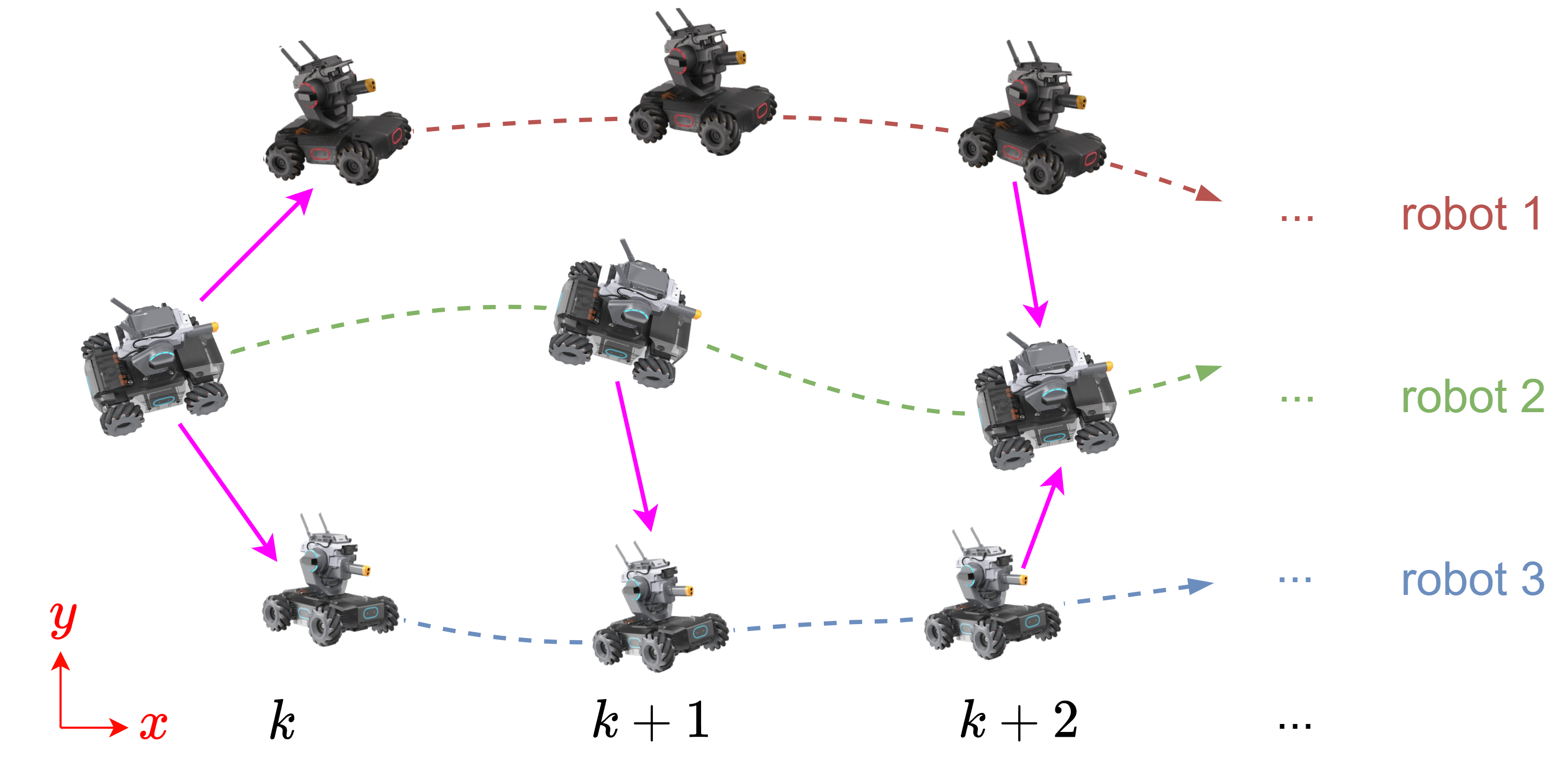
Figure 1: Example scenario of a multi-robot system performing cooperative localization. Dashed lines are the ego-motion information of each robot and purple arrows indicate robot-to-robot relative measurements.

Another method to avoid the double-counting problem is the EKF-based CL. The central EKF-based CL takes all the robot poses as the system state and utilizes one filter to estimate the system state. The correlations among the robot pose estimations are recorded by the cross-covariance matrices automatically. While EKF-based CL delivers the best localization accuracy, its naive distributed form [12] requires an all-to-all communication topology to update the cross-covariance matrices. To reduce the communication costs, [13] required only pairwise communication between two robots that obtain a relative measurement. However, the estimation consistency is sacrificed for the matrices that were approximated with block diagonal matrices. A central equivalent distributed CL algorithm named split-EKF was proposed in [14] and [15] which consists of a fusion center maintaining and updating cross-covariance matrices. Although EKF-based CL as well as its equivalent distributed forms [12], [14], [15], [16] avoid the double-counting problem, these methods still suffer from the inconsistency caused by the unobservable dimension reduction in [17, 18]. Because the absolute measurement is absent, the CL system is not completely observable. [19] have proved analytically that the linearized system employed by the EKF-based CL has an unobservable subspace of lower dimension than that of the nonlinear CL system. Consequently, the unobservable dimension reduction would result in the EKF-based CL becoming inconsistent, and thus the localization accuracy declines.

In this paper, a distributed consistent CL algorithm is proposed in which the state estimation EKF is performed in transformed coordinates and a server-assisted distributed framework is employed. In particular, a coordinate transformation is constructed by decomposing state-propagation Jacobian. The significance of the coordinate transformation is twofold. On the one hand, it guarantees that the transformed linearized error-state system has the same observability properties as that of the underlying nonlinear CL system. Thus, the inconsistency caused by the unobservable dimension reduction is eliminated in the proposed algorithm. On the other hand, the transformed state-propagation Jacobian becomes an identity matrix which is more suitable for distribution.

The main contributions of this paper are as follows:

• A coordinate transformation is constructed via decomposing the state-propagation Jacobian, by which the transformed linearized error-state system has the correct observability.

• A distributed server assistant EKF-based CL algorithm is proposed. The key idea is to perform state estimation EKF in the transformed coordinates. Since the correct observability properties are guaranteed, the consistency of the estimator is improved. Moreover, benefiting from the transformation, the transformed state-propagation Jacobian becomes an identity matrix such that the propagation and update of the cross-covariance matrices are significantly simplified.

• The proposed distributed CL algorithm is validated on the UTIAS dataset and the experiment results show that it has a better performance in terms of consistency and accuracy.

II Problem Formulation

In this section, we give the multi-robot cooperative localization system model and derive the linearized error-state system for EKF-based CL.

Consider a team of $N$ robots performing distributed cooperative localization on a 2D plane in which each robot is equipped with proprioceptive sensors to sense its ego-motion information and exteroceptive sensors to measure the relative measurement of other robots. An example scenario is shown in Fig. 1.

II-A System Model

Let $\boldsymbol{\rm{x}}_{i,k}$ be the pose of robot $i,i\in\{1,2,...,N\}$ in a common fixed frame at timestamp $k$, $\boldsymbol{\rm{x}}_{i,k}=\begin{bmatrix}\boldsymbol{\rm{p}}_{i,k}^{\top}&\theta_{i,k}\end{bmatrix}^{\top}$, where $\boldsymbol{\rm{p}}_{i,k}\in\mathbb{R}^{2}$ and $\theta_{i,k}\in\mathbb{R}$ are the position and orientation of robot $i$, respectively.

The motion of robot $i$ is described by

$$\small\begin{array}[]{rl}\boldsymbol{\rm{x}}_{i,k}&=\boldsymbol{\rm{x}}_{i,k-1}+\begin{bmatrix}\ {\boldsymbol{{\rm{C}}}}\left(\theta_{i,k-1}\right)&\bm{0}_{2\times 1}\\ \ \bm{0}_{1\times 2}&1\\ \end{bmatrix}({\boldsymbol{\rm{u}}}_{i,k-1}\Delta t+\bm{\epsilon}_{i,k-1})\\ &\triangleq\boldsymbol{{f}}_{i}\left(\boldsymbol{\rm{x}}_{i,k-1},{\boldsymbol{\rm{u}}}_{i,k-1},\bm{\epsilon}_{i,k-1}\right)\end{array}$$ (1)

where ${\boldsymbol{\rm{u}}}_{i,k-1}=\begin{bmatrix}\boldsymbol{\rm{v}}_{i,k-1}^{\top}&\omega_{i,k-1}\end{bmatrix}^{\top}$ , $\boldsymbol{\rm{v}}_{i,k-1}\in\mathbb{R}^{2}$ and $\omega_{i,k-1}\in\mathbb{R}$ are the linear and angular velocity of robot $i$, $\bm{\epsilon}_{i,k-1}\in\mathbb{R}^{3}$ denotes white Gaussian noise with ${\mathbb{E}}(\bm{\epsilon}_{i,k-1}\bm{\epsilon}_{i,k-1}^{\top})=\boldsymbol{\rm{Q}}_{i,k}>\bm{0}$. ${\boldsymbol{{\rm{C}}}}(\cdot)\in\mathbb{R}^{2\times 2}$ is the rotation matrix given by

$${\boldsymbol{{\rm{C}}}}(\cdot)=\begin{bmatrix}\cos(\cdot)&-\sin(\cdot)\\ \sin(\cdot)&\cos(\cdot)\\ \end{bmatrix}.$$

For the entire $N$-robot system, the state vector, motion input vector and process noise vector are defined as the column stacked vectors, i.e., $\small\boldsymbol{\rm{x}}_{k}=\begin{bmatrix}\boldsymbol{\rm{x}}_{1,k}^{\top}&\cdots&\boldsymbol{\rm{x}}_{N,k}^{\top}\par\par\end{bmatrix}^{\top}$, $\small\boldsymbol{\rm{u}}_{k}=\begin{bmatrix}\boldsymbol{\rm{u}}_{1,k}\top&\cdots&\boldsymbol{\rm{u}}_{N,k}^{\top}\end{bmatrix}^{\top}$ and $\small\bm{\epsilon}_{k}=\begin{bmatrix}\bm{\epsilon}_{1,k}^{\top}&\dots&\bm{\epsilon}_{N,k}^{\top}\end{bmatrix}^{\top}$. Then the system motion equation is given by

$$\boldsymbol{\rm{x}}_{k}=\boldsymbol{{f}}\left(\boldsymbol{\rm{x}}_{k-1},{\boldsymbol{\rm{u}}}_{k-1},\bm{\epsilon}_{k-1}\right)$$ (2)

For simplicity of expression, we assume that the $N$ robots obtain only one robot-to-robot relative measurement at timestamp $k$. Note that this assumption is not necessary for the proposed approach. Actually, any number of measurements is permitted. As for the case more than one measurement, a sequential update [20] can be employed.

If robot $\kappa,\kappa\in\{1,2,...,N\}$ obtains a robot-to-robot relative measurement of robot $\iota,\iota\in\{1,2,...,N\}/\kappa$, the measurement can be described by

$$\boldsymbol{\rm{y}}_{\kappa\iota,k}=\boldsymbol{{h}}(\boldsymbol{\rm{x}}_{\kappa,k},\boldsymbol{\rm{x}}_{\iota,k})+\bm{\varepsilon}_{\kappa\iota,k}\\$$ (3)

where $\boldsymbol{h}$ is allowed to be any function for robot-to-robot measurements such as relative bearing, relative distance, relative position or relative pose. $\bm{\varepsilon}_{\kappa\iota}$ is the measurement noise assumed to be the Gaussian white noise with $\small{\mathbb{E}}(\bm{\varepsilon}_{\kappa\iota,k}\bm{\varepsilon}_{\kappa\iota,k}^{\top})=\boldsymbol{\rm{R}}_{\kappa\iota,k}>\bm{0}$.

II-B Linearized Error-state System of EKF-based CL

Let $\hat{\boldsymbol{\rm{x}}}_{k}$ and $\boldsymbol{\rm{P}}_{k}$ be the estimation of $\boldsymbol{\rm{x}}_{k}$ and the corresponding covariance matrix, respectively. The error-state is $\tilde{\boldsymbol{\rm{x}}}_{k}\triangleq\boldsymbol{\rm{x}}_{k}-\hat{\boldsymbol{\rm{x}}}_{k}$. Linearizing (2) and (3), the linearized error-state system used by the EKF-based CL is given by

$$\tilde{\boldsymbol{\rm{x}}}_{k|k-1} =\boldsymbol{\rm{F}}_{k-1}\tilde{\boldsymbol{\rm{x}}}_{k-1|k-1}+\boldsymbol{\rm{G}}_{k-1}\bm{\epsilon}_{k-1}$$ (4a)

$${\tilde{\boldsymbol{\rm{y}}}}_{\kappa\iota} =\boldsymbol{\rm{H}}_{k}\tilde{\boldsymbol{\rm{x}}}_{k|k-1}+\bm{\varepsilon}_{\kappa\iota,k}$$ (4b)

where state-propagation Jacobian $\boldsymbol{\rm{F}}_{k-1}\in\mathbb{R}^{3N\times 3N}$ is a block diagonal matrix with the $i$-th diagonal block

$$\begin{array}[]{rl}\boldsymbol{\rm{F}}_{i,k-1}&=\frac{\partial\bm{f}_{i}}{\partial\boldsymbol{\rm{x}}_{i,k-1}}(\hat{\boldsymbol{\rm{x}}}_{i,k-1|k-1},\boldsymbol{\rm{u}}_{i,k-1},\bm{0})\\ &=\begin{bmatrix}\boldsymbol{\rm{I}}_{2\times 2}&\boldsymbol{\rm{J}}(\hat{\boldsymbol{\rm{p}}}_{i,k|k-1}-\hat{\boldsymbol{\rm{p}}}_{i,k-1|k-1})\\ \bm{0}_{1\times 2}&1\\ \end{bmatrix}\end{array}$$

with $\boldsymbol{\rm{J}}=\boldsymbol{{\rm{C}}}(\pi/2)$. The measurement Jacobian is

$$\boldsymbol{\rm{H}}_{k}=\begin{bmatrix}\bm{0}&\cdots&\boldsymbol{\rm{H}}_{\kappa,k}&\cdots&\boldsymbol{\rm{H}}_{\iota,k}&\cdots&\bm{0}\end{bmatrix}$$

with $\boldsymbol{\rm{H}}_{\kappa,k}=\frac{\partial\boldsymbol{h}}{\partial\boldsymbol{\rm{x}}_{\kappa,k}}(\hat{\boldsymbol{\rm{x}}}_{\kappa,k|k-1},\hat{\boldsymbol{\rm{x}}}_{\iota,k|k-1})$ and $\boldsymbol{\rm{H}}_{\iota,k}=\frac{\partial\boldsymbol{h}}{\partial\boldsymbol{\rm{x}}_{\iota,k}}(\hat{\boldsymbol{\rm{x}}}_{\kappa,k|k-1},\hat{\boldsymbol{\rm{x}}}_{\iota,k|k-1})$. $\boldsymbol{\rm{G}}_{k-1}\in\mathbb{R}^{3N\times 3N}$ is a block diagonal matrix with the $i$-th diagonal block

$$\begin{array}[]{rl}\boldsymbol{\rm{G}}_{i,k-1}&=\frac{\partial\bm{f}_{i}}{\partial\boldsymbol{\epsilon}_{i,k-1}}(\hat{\boldsymbol{\rm{x}}}_{i,k-1|k-1},\boldsymbol{\rm{u}}_{i,k-1},\bm{0})\\ &=\begin{bmatrix}\ {\boldsymbol{{\rm{C}}}}\left(\hat{\theta}_{i,k-1}\right)&\bm{0}_{2\times 1}\\ \ \bm{0}_{1\times 2}&1\\ \end{bmatrix}.\end{array}$$

Since the absolute pose information is not available, the non-linear system used by EKF-based CL has three unobservable dimensions, i.e., the absolute position and the orientation [21, 22]. [18] pointed out that the linearized error-state system (4) evaluated at the latest state estimates used by EKF-based CL has only two unobservable dimensions. In particular, the dimension corresponding to absolute orientation is mistakenly observable. It has been proved that the reduction of unobservable dimensions causes the inconsistency of the EKF-based CL. Consequently, the inconsistency results in localization accuracy decreasing. However, almost all the existing distributed methods do not take the issue into account. The aim of this paper is to propose a distributed consistent cooperative localization algorithm to address this issue.

III Coordinate Transformation

In this section, we first present the construction of the coordinate transformation. Then we derive the transformed error-state linearized system.

III-A Coordinate Transformation Design

The purpose of the coordinate transformation is to guarantee the dimension of the observable subspace of the transformed linearized system is identical to that of the original nonlinear CL system. Meanwhile, the transformed state-propagation and measurement Jacobian are expected to be as simple as possible.

We start by considering a linear time-varying discrete system:

$$\boldsymbol{\rm{x}}_{k} =\boldsymbol{\rm{A}}_{k-1}\boldsymbol{\rm{x}}_{k-1}+\boldsymbol{\rm{B}}_{k-1}\boldsymbol{\rm{n}}_{k-1}$$ (5a)

$$\boldsymbol{\rm{y}}_{k} =\boldsymbol{{\rm{C}}}_{k}\boldsymbol{\rm{x}}_{k}$$ (5b)

where $\boldsymbol{\rm{x}}_{k}\in\mathbb{R}^{n}$, $\boldsymbol{\rm{n}}_{k-1}\in\mathbb{R}^{l}$, $\boldsymbol{\rm{y}}_{k}\in\mathbb{R}^{m}$, $\boldsymbol{\rm{A}}_{k-1}\in\mathbb{R}^{n\times n}$, $\boldsymbol{\rm{B}}_{k-1}\in\mathbb{R}^{n\times l}$ and $\boldsymbol{{\rm{C}}}_{k}\in\mathbb{R}^{m\times n}$. A non-singular matrix $\boldsymbol{\mathcal{T}}_{k}\in\mathbb{R}^{n\times n}$ is called a coordinate transformation for system (5) [23], which yields $\boldsymbol{\rm{z}}_{k}=\boldsymbol{\mathcal{T}}_{k}\boldsymbol{\rm{x}}_{k}$ and

$$\boldsymbol{\rm{z}}_{k} =\boldsymbol{\mathcal{A}}_{k-1}\boldsymbol{\rm{z}}_{k-1}+\boldsymbol{\mathcal{B}}_{k-1}\boldsymbol{\rm{n}}_{k-1}$$ (6a)

$$\boldsymbol{\rm{y}}_{k} =\boldsymbol{\mathcal{C}}_{k}\boldsymbol{\rm{z}}_{k}$$ (6b)

where

$$\boldsymbol{\mathcal{A}}_{k-1} =\boldsymbol{\mathcal{T}}_{k}\boldsymbol{\rm{A}}_{k-1}\boldsymbol{\mathcal{T}}^{-1}_{k-1}$$ (7)

$$\boldsymbol{\mathcal{B}}_{k-1} =\boldsymbol{\mathcal{T}}_{k}\boldsymbol{\rm{B}}_{k-1}$$ (8)

$$\boldsymbol{\mathcal{C}}_{k} =\boldsymbol{{\rm{C}}}_{k}\boldsymbol{\mathcal{T}}_{k}^{-1}.$$ (9)

To figure out the ideal structure of the coordinate transformation for system (4), we decompose $\boldsymbol{\rm{F}}_{i,k-1}$ as follows

$$\small\begin{array}[]{rl}\boldsymbol{\rm{F}}_{i,k-1}&=\begin{bmatrix}\boldsymbol{\rm{I}}_{2\times 2}&\boldsymbol{\rm{J}}(\hat{\boldsymbol{\rm{p}}}_{i,k|k-1})\\ \bm{0}_{1\times 2}&1\end{bmatrix}\begin{bmatrix}\boldsymbol{\rm{I}}_{2\times 2}&-\boldsymbol{\rm{J}}(\hat{\boldsymbol{\rm{p}}}_{i,k-1|k-1})\\ \bm{0}_{1\times 2}&1\end{bmatrix}\\ &\triangleq\boldsymbol{\rm{T}}^{-1}_{i}(\hat{\boldsymbol{\rm{x}}}_{i,k|k-1})\boldsymbol{\rm{T}}_{i}(\hat{\boldsymbol{\rm{x}}}_{i,k-1|k-1}).\end{array}$$ (10)

Observing (7) and (10), we construct the coordinate transformation matrix ${\boldsymbol{\rm{T}}}(\hat{\boldsymbol{\rm{x}}}_{k})$ for system (4) as follows

$${\boldsymbol{\rm{T}}}(\hat{\boldsymbol{\rm{x}}}_{k})=\text{Diag}({\boldsymbol{\rm{T}}}_{1}(\hat{\boldsymbol{\rm{x}}}_{1,k}),...,{\boldsymbol{\rm{T}}}_{N}{(\hat{\boldsymbol{\rm{x}}}_{N,k})})$$ (11)

with

$${\boldsymbol{\rm{T}}}_{i}{(\hat{\boldsymbol{\rm{x}}}_{i,k})}=\begin{bmatrix}\boldsymbol{\rm{I}}_{2\times 2}&-\boldsymbol{\rm{J}}\hat{\boldsymbol{\rm{p}}}_{i,k}\\ 0_{1\times 2}&1\end{bmatrix},i\in\{1,2,...,N\}.$$ (12)

In the following, we will show that by the transformation (11), the transformed state-propagation Jacobian will become an identity matrix and the correct observability is guaranteed.

III-B Transformed linearized Error-state system

Now we derive the linearized error-state system in the transformed coordinates. Substituting $\boldsymbol{\rm{z}}_{k}={\boldsymbol{\rm{T}}}(\hat{\boldsymbol{\rm{x}}}_{k})\tilde{\boldsymbol{\rm{x}}}_{k}$ into (4) yields the transformed linearized error-state system as follows

$${\boldsymbol{\rm{z}}}_{k|k-1} =\boldsymbol{\mathcal{F}}_{k-1}{\boldsymbol{\rm{z}}}_{k-1|k-1}+\boldsymbol{\mathcal{G}}_{k-1}\bm{\epsilon}_{k-1}$$ (13a)

$$\tilde{\boldsymbol{\rm{y}}}_{\kappa\iota} =\boldsymbol{\mathcal{H}}_{k}{\boldsymbol{\rm{z}}}_{k|k-1}+\boldsymbol{\varepsilon}_{\kappa\iota,k}$$ (13b)

where

$$\boldsymbol{\mathcal{F}}_{k-1} ={\boldsymbol{\rm{T}}}(\hat{\boldsymbol{\rm{x}}}_{k|k-1})\boldsymbol{\rm{F}}_{k-1}{\boldsymbol{\rm{T}}}^{-1}(\hat{\boldsymbol{\rm{x}}}_{k-1|k-1})$$

$$=\boldsymbol{\rm{I}}_{3N\times 3N}$$

$$\boldsymbol{\mathcal{H}}_{k} =\boldsymbol{\rm{H}}_{k}{\boldsymbol{\rm{T}}}(\hat{\boldsymbol{\rm{x}}}_{k|k-1})^{-1}$$

$$=\begin{bmatrix}\bm{0}&\cdots&\boldsymbol{\mathcal{H}}_{\kappa,k}&\cdots&\boldsymbol{\mathcal{H}}_{\iota,k}&\cdots&\bm{0}\end{bmatrix}$$

$$\boldsymbol{\mathcal{G}}_{k-1} ={\boldsymbol{\rm{T}}}(\hat{\boldsymbol{\rm{x}}}_{k|k-1})\boldsymbol{\rm{G}}_{k-1}$$

with $\small{\boldsymbol{\mathcal{H}}_{\kappa,k}}=\boldsymbol{\rm{H}}_{\kappa,k}\boldsymbol{\rm{T}}_{\kappa}^{-1}(\hat{\boldsymbol{\rm{x}}}_{\kappa,k|k-1})$, $\small{\boldsymbol{\mathcal{H}}_{\iota,k}}=\boldsymbol{\rm{H}}_{\iota,k}\boldsymbol{\rm{T}}_{\iota}^{-1}(\hat{\boldsymbol{\rm{x}}}_{\iota,k|k-1})$.

Remark 1

The transformed state-propagation Jacobian $\boldsymbol{\mathcal{F}}_{k}$ is an identity matrix, which is more suitable for distribution. Specifically, the propagation and update of the cross-covariance matrix are significantly simplified in distributed CL.

Lemma 1

The dimension of the observable subspace of transformed error-state system (13) is the same as that of the non-linear CL system.

Proof:

It has been proved that the observable dimension of the nonlinear CL system is $3N-3$ in [21] and [22]. Since $\boldsymbol{\mathcal{F}}_{k-1}=\boldsymbol{\rm{I}}_{3N\times 3N}$, the dimension of the observable subspace of system (13) is equal to the rank of $\boldsymbol{\mathcal{H}}_{k}$. It can be checked easily that $\text{rank}(\boldsymbol{\mathcal{H}}_{k})=3N-3$, which completes the proof. ∎

IV Distributed CL algorithm

In this section, we propose a distributed consistent CL algorithm. The key idea is to perform the state estimation EKF by using the transformed linearized error-state system (13). To achieve a distributed algorithm, we adopt a server-assistant framework in which each robot stores and propagates its pose estimation while the server maintains the cross-covariance matrices. A scheme of the proposed distributed CL algorithm is shown in Fig. 2.

Figure 2: The proposed distributed CL algorithm that runs on the server and each robot $i,\quad i,j\in\{1,2,\dots,N\},j\neq i$. The purple arrow represents the relative measurement between robot $\kappa,\kappa\in\{1,2,\dots,N\}$ and $\iota,\iota\in\{1,2,\dots,N\}/\kappa$ and the black arrow represents the communication between the server and the robots.

IV-A Algorithm Details

In the proposed CL algorithm, each robot $i$ stores and propagates its local estimation $(\hat{\boldsymbol{\rm{x}}}_{i,k},\boldsymbol{\mathcal{P}}_{ii,k})$ and the server maintains all the off-diagonal blocks in $\boldsymbol{\mathcal{P}}_{k}$, i.e., the transformed cross-covariance matrices $\{\boldsymbol{\mathcal{P}}_{ij,k}\}_{i\neq j}$. When the measurement $\boldsymbol{\rm{y}}_{\kappa\iota,k}$ is taken, robot $\kappa$ and robot $\iota$ send their local estimates to the server. Then all robots receive the information from the server to update their local estimations. The details of each algorithm step are as follows.

(1) Initialization: Let $\boldsymbol{\rm{P}}_{0}$ denote the joint covariance matrix corresponding to the initial estimation $\hat{\boldsymbol{\rm{x}}}_{0}$. $\boldsymbol{\rm{P}}_{0}$ is transformed into $\boldsymbol{\mathcal{P}}_{0}$ by

$$\boldsymbol{\mathcal{P}}_{0}={\boldsymbol{\rm{T}}}(\hat{\boldsymbol{\rm{x}}}_{0})\boldsymbol{\rm{P}}_{0}{\boldsymbol{\rm{T}}}(\hat{\boldsymbol{\rm{x}}}_{0})^{\top}.$$ (14)

All the robots’ poses are assumed to be uncorrelated at time $k=0$, i.e., $\boldsymbol{\rm{P}}_{0}$ is a diagonal block matrix. According to (14), $\boldsymbol{\mathcal{P}}_{0}$ is also a diagonal block matrix.

Server: Set all the off-diagonal blocks in $\boldsymbol{\mathcal{P}}_{0}$, i.e., cross-covariance matrices $\{\boldsymbol{\mathcal{P}}_{ij,0}\}_{i\neq j}$ be $\bm{0}$.

Robot $i$: Transform its covariance matrix $\boldsymbol{\rm{P}}_{ii,0}$ into $\boldsymbol{\mathcal{P}}_{ii,0}$

$$\boldsymbol{\mathcal{P}}_{ii,0}={\boldsymbol{\rm{T}}}_{i}(\hat{\boldsymbol{\rm{x}}}_{i,0})\boldsymbol{\rm{P}}_{ii,0}{\boldsymbol{\rm{T}}}_{i}(\hat{\boldsymbol{\rm{x}}}_{i,0})^{\top}.$$ (15)

(2) Propagation: The propagation of the transformed covariance matrix $\boldsymbol{\mathcal{P}}_{k}$ is given by

$$\boldsymbol{\mathcal{P}}_{k|k-1} =\boldsymbol{\mathcal{F}}_{k-1}\boldsymbol{\mathcal{P}}_{k-1|k-1}\boldsymbol{\mathcal{F}}_{k-1}^{\top}+\boldsymbol{\mathcal{G}}_{k-1}\boldsymbol{\rm{Q}}_{k}\boldsymbol{\mathcal{G}}_{k-1}^{\top}.$$ (16)

Note that only diagonal blocks in $\boldsymbol{\mathcal{P}}_{k}$ need to be propagated since $\boldsymbol{\mathcal{F}}_{k-1}$ is an identity matrix and $\boldsymbol{\mathcal{G}}_{k-1}\boldsymbol{\rm{Q}}_{k}\boldsymbol{\mathcal{G}}_{k-1}^{\top}$ in (16) is a diagonal block matrix,

Server: Remain the cross-covariance matrices $\{\boldsymbol{\mathcal{P}}_{ij,k}\}_{i\neq j}$ unchanged, i.e.

$$\boldsymbol{\mathcal{P}}_{ij,k|k-1}=\boldsymbol{\mathcal{P}}_{ij,k-1|k-1}.$$ (17)

Robot $i$: Propagate its local estimation as

$$\hat{\boldsymbol{\rm{x}}}_{i,k|k-1} =\boldsymbol{f}_{i}\left(\hat{\boldsymbol{\rm{x}}}_{i,k-1|k-1},{\boldsymbol{\rm{u}}}_{i,k-1},\bm{0}\right)$$ (18a)

$$\boldsymbol{\mathcal{P}}_{ii,k|k-1} =\boldsymbol{\mathcal{P}}_{ii,k-1|k-1}+\boldsymbol{\mathcal{G}}_{i,k-1}\boldsymbol{\rm{Q}}_{i,k-1}\boldsymbol{\mathcal{G}}_{i,k-1}^{\top}$$ (18b)

where

$$\boldsymbol{\mathcal{G}}_{i,k-1}={\boldsymbol{\rm{T}}}_{i}(\hat{\boldsymbol{\rm{x}}}_{i,k|k-1})\boldsymbol{\rm{G}}_{i,k-1}.$$ (19)

(3) Update: The update steps in the transformed coordinates are

$$\boldsymbol{\mathcal{S}}_{\kappa\iota} =\boldsymbol{\mathcal{H}}_{k}\boldsymbol{\mathcal{P}}_{k}\boldsymbol{\mathcal{H}}_{k}^{\top}+\boldsymbol{\rm{R}}_{\kappa\iota,k}$$ (20a)

$$\boldsymbol{\mathcal{K}} =\boldsymbol{\mathcal{P}}_{k|k-1}\boldsymbol{\mathcal{H}}_{k}^{\top}\boldsymbol{\mathcal{S}}_{\kappa\iota}^{-1}$$ (20b)

$$\boldsymbol{\rm{z}}_{k|k} =\boldsymbol{\rm{z}}_{k|k-1}+\boldsymbol{\mathcal{K}}\tilde{\boldsymbol{\rm{y}}}_{\kappa\iota}$$ (20c)

$$\boldsymbol{\mathcal{P}}_{k|k} =\boldsymbol{\mathcal{P}}_{k|k-1}-\boldsymbol{\mathcal{K}}\boldsymbol{\mathcal{H}}_{k}\boldsymbol{\mathcal{P}}_{k|k-1}.$$ (20d)

From (20c), the updated equation for $\hat{\boldsymbol{\rm{x}}}_{k}$ is

$$\begin{array}[]{rl}\hat{\boldsymbol{\rm{x}}}_{k|k}&=\hat{\boldsymbol{\rm{x}}}_{k|k-1}+{\boldsymbol{\rm{T}}}^{-1}(\hat{\boldsymbol{\rm{x}}}_{k|k-1})(\boldsymbol{\rm{z}}_{k|k}-\boldsymbol{\rm{z}}_{k|k-1})\\ &=\hat{\boldsymbol{\rm{x}}}_{k|k-1}+{\boldsymbol{\rm{T}}}^{-1}(\hat{\boldsymbol{\rm{x}}}_{k|k-1})\boldsymbol{\mathcal{K}}\tilde{\boldsymbol{\rm{y}}}_{\kappa\iota}.\end{array}$$ (21)

To obtain the update for the server and each robot, we need to decompose (20d) and (21).

Server: Once robot $\kappa$ obtains a relative measurement from robot $\iota$, the server receives $\hat{\boldsymbol{\rm{x}}}_{\kappa,k|k-1},\boldsymbol{\mathcal{P}}_{\kappa\kappa,k|k-1}$, $\boldsymbol{\rm{y}}_{\kappa\iota,k}$ from robot $\kappa$ and $\hat{\boldsymbol{\rm{x}}}_{\iota,k|k-1},\boldsymbol{\mathcal{P}}_{\iota\iota,k|k-1}$ from robot $\iota$.Then $\tilde{\boldsymbol{\rm{y}}}_{\kappa\iota}$,$\boldsymbol{\mathcal{H}}_{\kappa,k}$ and $\boldsymbol{\mathcal{H}}_{\iota,k}$ can be calculated. Then the innovation covariance matrix can be obtained by

$$\begin{array}[]{rcl}\boldsymbol{\mathcal{S}}_{\kappa\iota}&=&\boldsymbol{\mathcal{H}}_{k}\boldsymbol{\mathcal{P}}_{k}\boldsymbol{\mathcal{H}}_{k}^{\top}+\boldsymbol{\rm{R}}_{\kappa\iota,k}\\ &=&\boldsymbol{\mathcal{H}}_{\kappa,k}\boldsymbol{\mathcal{P}}_{\kappa\kappa,k|k-1}\boldsymbol{\mathcal{H}}_{\kappa,k}^{\top}+\boldsymbol{\mathcal{H}}_{\kappa,k}\boldsymbol{\mathcal{P}}_{\kappa\iota,k|k-1}\boldsymbol{\mathcal{H}}_{\iota,k}^{\top}\\ &+&\boldsymbol{\mathcal{H}}_{\iota,k}\boldsymbol{\mathcal{P}}_{\iota\kappa,k|k-1}\boldsymbol{\mathcal{H}}_{\kappa,k}^{\top}+\boldsymbol{\mathcal{H}}_{\iota,k}\boldsymbol{\mathcal{P}}_{\iota\iota,k|k-1}\boldsymbol{\mathcal{H}}_{\iota,k}^{\top}+\boldsymbol{\rm{R}}_{\kappa\iota,k}\end{array}.$$ (22)

The cross-covariance stored in the server is updated as

$$\boldsymbol{\mathcal{P}}_{ij,k|k}=\boldsymbol{\mathcal{P}}_{ij,k|k-1}-\boldsymbol{\mathcal{D}}_{i}\boldsymbol{\mathcal{S}}_{\kappa\iota}^{-1}\boldsymbol{\mathcal{D}}_{j}^{\top}$$ (23)

where

$$\ \small\boldsymbol{\mathcal{D}}_{i}=\boldsymbol{\mathcal{P}}_{i\kappa,k|k-1}\boldsymbol{\mathcal{H}}_{\kappa,k}^{\top}+\boldsymbol{\mathcal{P}}_{i\iota,k|k-1}\boldsymbol{\mathcal{H}}_{\iota,k}^{\top}\quad i\in\{1,2,...,N\}.$$ (24)

Note the server only needs to update the upper triangular blocks in $\boldsymbol{\mathcal{P}}_{k}$, i.e., $\{\boldsymbol{\mathcal{P}}_{ij,k}\}_{i\in\{1,2,...,N-1\},j\in\{i+1,i+2,...,N\}}$ since the matrix $\boldsymbol{\mathcal{P}}_{k}$ is symmetric.

Robot $i$: Update its local estimation by

$$\hat{\boldsymbol{\rm{x}}}_{i,k|k} =\hat{\boldsymbol{\rm{x}}}_{i,k|k-1}+{\boldsymbol{\rm{T}}}_{i}^{-1}(\hat{\boldsymbol{\rm{x}}}_{i,k|k-1})\boldsymbol{\mathcal{D}}_{i}\boldsymbol{\mathcal{S}}_{\kappa\iota}^{-1}\tilde{\boldsymbol{\rm{y}}}_{\kappa\iota}$$ (25a)

$$\boldsymbol{\mathcal{P}}_{ii,k|k} =\boldsymbol{\mathcal{P}}_{iik|k-1}-\boldsymbol{\mathcal{D}}_{i}\boldsymbol{\mathcal{S}}_{\kappa\iota}^{-1}\boldsymbol{\mathcal{D}}_{i}^{\top}$$ (25b)

by using the information $\small\boldsymbol{\mathcal{D}}_{i}\boldsymbol{\mathcal{S}}_{\kappa\iota}^{-1}\tilde{\boldsymbol{\rm{y}}}_{\kappa\iota},\boldsymbol{\mathcal{D}}_{i}\boldsymbol{\mathcal{S}}_{\kappa\iota}^{-1}\boldsymbol{\mathcal{D}}_{i}^{\top}$ received from the server.

The pseudocode is shown in Algorithm 1.

Input: $\{\boldsymbol{\rm{u}}_{1,k-1},\boldsymbol{\rm{u}}_{2,k-1},\dots,\boldsymbol{\rm{u}}_{N,k-1}\}$,$\boldsymbol{\rm{y}}_{\kappa\iota,k}$

Output: $\{(\hat{\boldsymbol{\rm{x}}}_{1,k},\boldsymbol{\rm{P}}_{11,k}),...,(\hat{\boldsymbol{\rm{x}}}_{N,k},\boldsymbol{\rm{P}}_{NN,k})\}$

// $i\neq j\quad i,j\in\{1,2,...,N\}$

// Initialization at $k=0$

Server :	$\boldsymbol{\mathcal{P}}_{ij,0}=\bm{0}$
Robot $i$ :	$\hat{\boldsymbol{\rm{x}}}_{i,0}\in\mathbb{R}^{3},\quad\boldsymbol{\mathcal{P}}_{ii,0}={\boldsymbol{\rm{T}}}_{i}(\hat{\boldsymbol{\rm{x}}}_{i,0})\boldsymbol{\rm{P}}_{ii,0}{\boldsymbol{\rm{T}}}_{i}(\hat{\boldsymbol{\rm{x}}}_{i,0})^{\top}$

// Propagation when each robot $i$ gets its motion input $\boldsymbol{\rm{u}}_{i,k-1}$

Server :	$\boldsymbol{\mathcal{P}}_{ij,k|k-1}=\boldsymbol{\mathcal{P}}_{ij,k-1|k-1}$
Robot $i$ :
$\hat{\boldsymbol{\rm{x}}}_{i,k|k-1}=\boldsymbol{f}_{i}\left(\hat{\boldsymbol{\rm{x}}}_{i,k-1|k-1},{\boldsymbol{\rm{u}}}_{i,k-1},\bm{0}\right)$
calculate $\boldsymbol{\mathcal{G}}_{i,k-1}$ using (19)

      $\small\boldsymbol{\mathcal{P}}_{ii,k|k-1}=\boldsymbol{\mathcal{P}}_{ii,k-1|k-1}+\boldsymbol{\mathcal{G}}_{i,k-1}\boldsymbol{\rm{Q}}_{i,k-1}\boldsymbol{\mathcal{G}}_{i,k-1}^{\top}$

// Update when robot $\kappa$ obtains a measurement $\boldsymbol{\rm{y}}_{\kappa\iota,k}$ from robot $\iota$

Server :
receive $(\hat{\boldsymbol{\rm{x}}}_{\kappa,k|k-1},\boldsymbol{\mathcal{P}}_{\kappa\kappa,k|k-1})$ and $\boldsymbol{\rm{y}}_{\kappa\iota,k}$ from robot $\kappa$
receive $(\hat{\boldsymbol{\rm{x}}}_{\iota,k|k-1},\boldsymbol{\mathcal{P}}_{\iota\iota,k|k-1})$ from robot $\iota$
calculate measurement residual $\tilde{\boldsymbol{\rm{y}}}_{\kappa\iota}$
calculate $\boldsymbol{\mathcal{S}}_{\kappa\iota}$ using (22)
calculate $\{\boldsymbol{\mathcal{D}}_{1},\boldsymbol{\mathcal{D}}_{2},...,\boldsymbol{\mathcal{D}}_{N}\}$ using (24)
$\boldsymbol{\mathcal{P}}_{ij,k|k}=\boldsymbol{\mathcal{P}}_{ij,k|k-1}-\boldsymbol{\mathcal{D}}_{i}\boldsymbol{\mathcal{S}}_{\kappa\iota}^{-1}\boldsymbol{\mathcal{D}}_{j}^{\top}$

Robot $i$ :     receive $(\boldsymbol{\mathcal{D}}_{i}\boldsymbol{\mathcal{S}}_{\kappa\iota}^{-1}\tilde{\boldsymbol{\rm{y}}}_{\kappa\iota},\boldsymbol{\mathcal{D}}_{i}\boldsymbol{\mathcal{S}}_{\kappa\iota}^{-1}\boldsymbol{\mathcal{D}}_{i}^{\top})$ from Server     $\hat{\boldsymbol{\rm{x}}}_{i,k|k}=\hat{\boldsymbol{\rm{x}}}_{i,k|k-1}+{\boldsymbol{\rm{T}}}_{i}^{-1}(\hat{\boldsymbol{\rm{x}}}_{i,k|k-1})\boldsymbol{\mathcal{D}}_{i}\boldsymbol{\mathcal{S}}_{\kappa\iota}^{-1}\tilde{\boldsymbol{\rm{y}}}_{\kappa\iota}$     $\boldsymbol{\mathcal{P}}_{ii,k|k}=\boldsymbol{\mathcal{P}}_{ii,k|k-1}-\boldsymbol{\mathcal{D}}_{i}\boldsymbol{\mathcal{S}}_{\kappa\iota}^{-1}\boldsymbol{\mathcal{D}}_{i}^{\top}$

IV-B Algorithm Properties

Compared to EKF-based CL, the consistency of the proposed distributed algorithm is improved.

Lemma 2

The inconsistency caused by the unobservable dimension reduction is eliminated in the proposed distributed algorithm.

Proof:

The proposed algorithm performs the state estimation EKF in the transformed coordinates in which the correct observability is guaranteed, i.e. the structure and dimension of the unobservable subspace are the same as that of the underlying nonlinear CL system, which immediately completes the proof.

∎

In addition, the proposed CL algorithm is fully distributed in the propagation steps since no communication is required between the robots and the server in the propagation steps.

V experimental results

In this section, we compare the proposed algorithm with the following three state-of-the-art EKF-based distributed cooperative localization algorithms, SA[15], BDA[9] and DMV[13].

We test the aforementioned four algorithms on a publicly available dataset, the UTIAS dataset [24]. This dataset consists of nine different subdatasets, each lasting 15 to 70 minutes. Each subdataset records the odometry, measurements, and pose ground truth of $N=5$ robots. Each robot measures relative bearing and range with respect to the other 4 robots and up to 15 landmarks with known identities.

These four algorithms are tested using the whole duration data of all UTIAS subdatasets. The relative bearing and range measurements between robots are used as the relative position measurements and odometry is used as the motion input. The pose estimation of each robot is initialized with the ground truth.

The estimation errors of the robot $1$ on subdataset 1 and 2 are displayed as an illustration in Fig. 3.

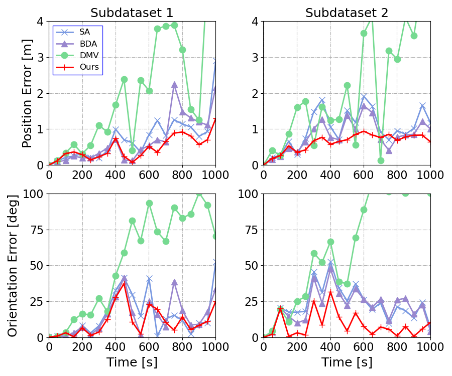
Figure 3: Robot $1$ estimation errors in the first 1000s on the UTIAS subdataset 1 and subdataset 2.

One can see that the proposed algorithm outperforms the other three algorithms in both position and orientation accuracy almost over the entire duration. A more challenging scenario is presented in subdataset 9, where barriers are placed in the workplace and occasionally obstruct observations. To avoid the incorrect ground truth data at the beginning, we present the position estimation errors from 1500 seconds, as shown in Fig. 4.

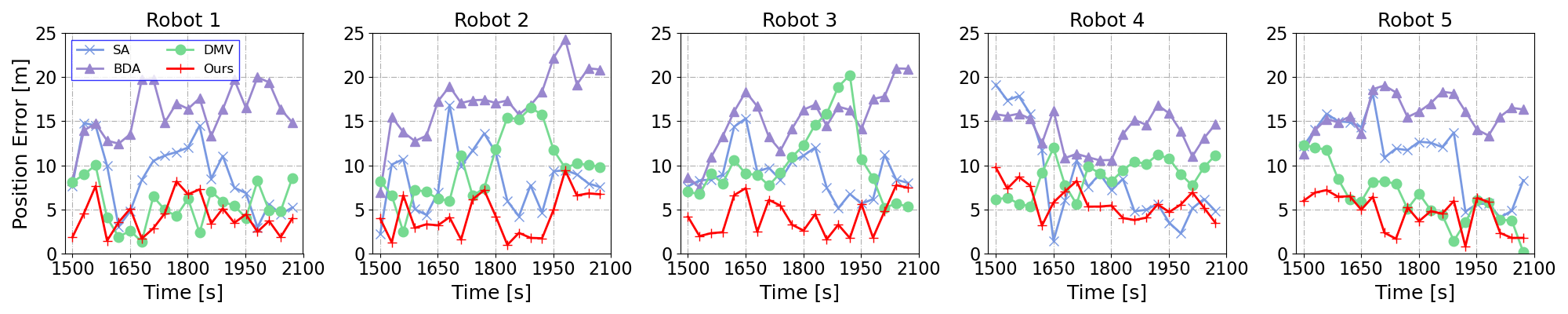
Figure 4: 5 robot position estimation errors in the last 600s on the UTIAS subdataset 9

From Fig. 4 we can see that the proposed algorithm has better positioning performance on subdataset 9 compared with other algorithms.

TABLE I: RMSE and NEES on the UTIAS datasets

Subdataset #		$\text{RMSE}_{\boldsymbol{\rm{p}}}$ [m]	$\text{RMSE}_{\theta}$ [deg]	NEES
	SA	1.00	25.76	8.37
1	BDA	1.28	25.87	98.14
(1487s)	DMV	2.42	55.91	1.24
	Ours	0.74	22.80	2.56
	SA	1.15	21.03	10.87
2	BDA	0.84	18.80	51.06
(1847s)	DMV	3.06	81.60	1.63
	Ours	0.67	11.50	2.69
	SA	0.60	14.83	3.38
3	BDA	0.55	14.47	11.00
(1502s)	DMV	2.57	57.88	1.77
	Ours	0.34	24.92	1.18
	SA	1.92	56.84	61.42
4	BDA	1.44	40.75	190.19
(1382s)	DMV	2.43	87.70	3.10
	Ours	0.80	16.14	3.53
	SA	0.64	11.13	2.51
5	BDA	0.70	15.68	33.85
(2292s)	DMV	2.66	72.52	0.98
	Ours	0.80	11.04	1.97
	SA	0.75	20.39	6.85
6	BDA	0.86	20.78	63.78
(756s)	DMV	2.41	65.48	2.05
	Ours	0.38	10.44	1.28
	SA	0.89	16.68	7.69
7	BDA	1.08	20.82	72.85
(891s)	DMV	2.18	69.04	2.59
	Ours	0.83	9.81	5.26
	SA	4.64	78.05	99.40
8	BDA	3.93	73.41	1031.29
(4192s)	DMV	5.01	104.99	2.23
	Ours	0.90	25.29	1.86
	SA	3.15	67.99	131.49
9	BDA	3.03	70.30	228.35
(2099s)	DMV	3.87	86.85	24.74
	Ours	2.40	57.21	54.13

The Root Mean Square Error (RMSE) is widely utilized to evaluate the accuracy of an estimator. We calculate the $N=5$ robots average $\text{RMSE}_{\boldsymbol{\rm{p}}}$ and $\text{RMSE}_{\theta}$ overall one subdataset’s timesteps. The Normalized estimation error squared (NEES) is a metric to evaluate the consistency of these algorithms, we calculate NEES on a subdataset as

$$\small\text{NEES}=\frac{1}{NT}\sum_{i=1}^{N}\sum_{k=1}^{T}(\boldsymbol{\rm{x}}_{i,k}-\hat{\boldsymbol{\rm{x}}}_{i,k|k})^{\top}\boldsymbol{\rm{P}}_{ii,k}^{-1}(\boldsymbol{\rm{x}}_{i,k}-\hat{\boldsymbol{\rm{x}}}_{i,k|k})$$ (26)

where P_ii,k = T_i^-1(^x _i,k) P_ii,k (T_i^-1(^x _i,k))^⊤. The consistency of an algorithm is better if its NEES is closer to 3, i.e., the dimension of the robot state.

The RMSE and NEES of these four algorithms are shown in Table I. On almost all the 9 subdatasets (except 3 and 5), the proposed algorithm has both the smallest position and orientation RMSE. DMV has the best NEES on subdataset 4, 6, 7, 8 and 9. The proposed algorithm has the best NEES on subdataset 1, 2 and has the competitive NEES (closest to the NEES of DMV) on the other subdatasets (except 3 and 5).

VI Conclusion

In this paper, we constructed a coordinate transformation by decomposing the state-propagation Jacobian. The transformation not only guarantees the transformed linearized error-state system has the same observability properties as that of the nonlinear CL system but also makes it more simple to propagate and update cross-covariance matrices in distributed CL. We propose a distributed consistent CL algorithm in which the state estimations are performed in the transformed coordinates. This guarantees that the inconsistency caused by unobservable dimension reduction is eliminated. By comparing with the state-of-art algorithms on the UTIAS dataset, the proposed CL algorithm shows better performance in terms of consistency and localization accuracy.

A. Bahr, M. R. Walter, and J. J. Leonard, “Consistent cooperative localization,” in Proceedings - IEEE International Conference on Robotics and Automation, 2009, pp. 3415–3422.

S. Julier and J. Uhlmann, “A non-divergent estimation algorithm in the presence of unknown correlations,” in Proceedings of the 1997 American Control Conference (Cat. No.97CH36041), vol. 4, Jun. 1997, pp. 2369–2373 vol.4.

L. C. Carrillo-Arce, E. D. Nerurkar, J. L. Gordillo, and S. I. Roumeliotis, “Decentralized multi-robot cooperative localization using covariance intersection,” in IEEE International Conference on Intelligent Robots and Systems, 2013, pp. 1412–1417.

T. K. Chang, K. Chen, and A. Mehta, “Resilient and Consistent Multirobot Cooperative Localization with Covariance Intersection,” IEEE Transactions on Robotics, vol. 38, no. 1, pp. 197–208, Feb. 2022.

J. Sijs and M. Lazar, “State fusion with unknown correlation: Ellipsoidal intersection,” Automatica, vol. 48, no. 8, pp. 1874–1878, Aug. 2012.

H. Li, F. Nashashibi, and M. Yang, “Split Covariance Intersection Filter: Theory and Its Application to Vehicle Localization,” IEEE Transactions on Intelligent Transportation Systems, vol. 14, no. 4, pp. 1860–1871, Dec. 2013.

B. Noack, J. Sijs, M. Reinhardt, and U. D. Hanebeck, “Decentralized data fusion with inverse covariance intersection,” Automatica, vol. 79, pp. 35–41, May 2017.

J. Zhu and S. S. Kia, “Cooperative Localization under Limited Connectivity,” IEEE Transactions on Robotics, vol. 35, no. 6, pp. 1523–1530, Dec. 2019.

C. Chen and S. S. Kia, “Cooperative Localization Using Learning-Based Constrained Optimization,” IEEE Robotics and Automation Letters, vol. 7, no. 3, pp. 7052–7058, Jul. 2022.

S. Leonardos and K. Daniilidis, “A game-theoretic approach to Robust Fusion and Kalman filtering under unknown correlations,” in 2017 American Control Conference (ACC), May 2017, pp. 2568–2573.

S. Roumeliotis and G. Bekey, “Distributed multirobot localization,” IEEE Transactions on Robotics and Automation, vol. 18, no. 5, pp. 781–795, Oct. 2002.

L. Luft, T. Schubert, S. I. Roumeliotis, and W. Burgard, “Recursive decentralized localization for multi-robot systems with asynchronous pairwise communication,” The International Journal of Robotics Research, vol. 37, no. 10, pp. 1152–1167, Sep. 2018.

S. S. Kia, S. Rounds, and S. Martínez, “Cooperative localization under message dropouts via a partially decentralized EKF scheme,” in 2015 IEEE International Conference on Robotics and Automation (ICRA), May 2015, pp. 5977–5982.

S. S. Kia, J. Hechtbauer, D. Gogokhiya, and S. Martínez, “Server-Assisted Distributed Cooperative Localization Over Unreliable Communication Links,” IEEE Transactions on Robotics, vol. 34, no. 5, pp. 1392–1399, Oct. 2018.

K. Y. K. Leung, T. D. Barfoot, and H. H. T. Liu, “Decentralized Localization of Sparsely-Communicating Robot Networks: A Centralized-Equivalent Approach,” IEEE Transactions on Robotics, vol. 26, no. 1, pp. 62–77, Feb. 2010.

G. P. Huang, A. I. Mourikis, and S. I. Roumeliotis, “Analysis and improvement of the consistency of extended Kalman filter based SLAM,” in 2008 IEEE International Conference on Robotics and Automation, May 2008, pp. 473–479.

G. P. Huang, N. Trawny, A. I. Mourikis, and S. I. Roumeliotis, “Observability-based consistent EKF estimators for multi-robot cooperative localization,” Autonomous Robots, vol. 30, no. 1, pp. 99–122, Jan. 2011.

N. Hao, F. He, C. Tian, Y. Yao, and S. Mou, “Kd-ekf: A kalman decomposition based extended kalman filter for multi-robot cooperative localization,” arXiv preprint arXiv:2210.16086, 2022.

J. van Genderen, “Tracking and data fusion: a handbook of algorithms, by yaakov bar-shalom, peter k. willett and xin tian,” International Journal of Image and Data Fusion, vol. 4, no. 1, pp. 102–104, 2013.

N. Hao, F. He, Y. Hou, and Y. Yao, “Graph-based observability analysis for mutual localization in multi-robot systems,” Systems & Control Letters, vol. 161, p. 105152, Mar. 2022.

N. Hao, F. He, C. Xie, C. Tian, and Y. Yao, “Nonlinear observability analysis of multi-robot cooperative localization,” Systems & Control Letters, vol. 168, p. 105340, Oct. 2022.

G. Gu, “Linear System Theory,” in Discrete-Time Linear Systems: Theory and Design with Applications, G. Gu, Ed., Boston, MA, 2012, pp. 67–124.

K. Y. Leung, Y. Halpern, T. D. Barfoot, and H. H. Liu, “The utias multi-robot cooperative localization and mapping dataset,” The International Journal of Robotics Research, vol. 30, no. 8, pp. 969–974, 2011.

Algorithm 1 the proposed distributed consitent CL