A general Bayesian approach to design adaptive clinical trials with time-to-event outcomes

Abstract

Clinical trials are an integral component of medical research. Trials require careful design to, for example, maintain the safety of participants, use resources efficiently and allow clinically meaningful conclusions to be drawn. Adaptive clinical trials (i.e. trials that can be altered based on evidence that has accrued) are often more efficient, informative and ethical than standard or non-adaptive trials because they require fewer participants, target more promising treatments, and can stop early with sufficient evidence of effectiveness or harm. The design of adaptive trials requires the pre-specification of adaptions that are permissible throughout the conduct of the trial. Proposed adaptive designs are then usually evaluated through simulation which provides indicative metrics of performance (e.g. statistical power and type-1 error) under different scenarios. Trial simulation requires assumptions about the data generating process to be specified but correctly specifying these in practice can be difficult, particularly for new and emerging diseases. To address this, we propose an approach to design adaptive clinical trials without needing to specify the complete data generating process. To facilitate this, we consider a general Bayesian framework where inference about the treatment effect on a time-to-event outcome can be performed via the partial likelihood. As a consequence, the proposed approach to evaluate trial designs is robust to the specific form of the baseline hazard function. The benefits of this approach are demonstrated through the redesign of a recent clinical trial to evaluate whether a third dose of a vaccine provides improved protection against gastroenteritis in Australian Indigenous infants.

Keywords: Bayesian design; Effectiveness; Futility; General Bayesian design; Partial likelihood; Proportional hazards; Robust design; Sequential design

1 Introduction

The outbreak of COVID-19 has brought about an unprecedented push to undertake clinical trial assessments as quickly as possible. Adaptive trials are particularly appealing in this regard because, based on the analysis of accruing data, without compromising the scientific rigour or the validity of the trial [6]: (1) the trial can stop early due to success or futility; (2) a treatment can be dropped from the trial if it is deemed ineffective or unsafe; (3) new treatments can be included mid-trial as new therapies emerge; and (4) treatments can be allocated such that the most promising are allocated more often (on average), see [28] for more examples of how a trial can adapt. Accordingly, when compared to fixed or less flexible trials, adaptive trials can complete sooner, cost less to run and reduce the number of participants on inferior treatments [8, 36]. In designing such trials, rules for adjusting or stopping the trial need to be determined a priori based on assumptions about potential effect sizes and the likely data that will be observed. If these assumptions are misspecified, then incorrect conclusions about treatment effects can be made as a result of the design [34]. This presents significant challenges for adaptive trials as there can be considerable uncertainty about the onset, course and resolution of the disease. To address this, we propose a new approach to design adaptive clinical trials which have time-to-event outcomes based on the partial likelihood that accordingly does not require specifying the complete data generating process. Our approach is applied to redesign a recent clinical trial where the benefits of our approach are demonstrated.

The focus of this paper is Bayesian methods to design adaptive trials. This is motivated by the framework providing a natural approach to update prior information as data are accrued, and the rigorous handling of uncertainty about, for example, missing data. The typical approach to design such trials is to ascertain prior information about the treatment effect and the data generating process for the outcome of interest, then to simulate a large number of hypothetical trials to derive empirical estimates of metrics that provide insight into the performance of the design such as Bayesian analogues of statistical power and type-1 error [16]. The trial design can then be modified to optimise these performance metrics in some way. The literature on Bayesian adaptive trial design is extensive, so we will not provide a comprehensive review here. Instead, we provide a brief summary below, and direct readers to a recent review given by [12] and the seminal text by [3].

Possibly the most well known Bayesian adaptive design approach is the Continual Reassessment Method (CRM) given by [25] which aims to find the dose that corresponds to a particular quantile of a dose-response relationship. Since this seminal publication, many variations and extensions have been proposed including patient specific dosing [1], assessing multiple drugs in combination [39] and using CRM in combination with other design approaches [23]. CRM appears to be used most commonly to design oncology trials e.g. [19]. Other adaptive designs where the probability of receiving a treatment can vary depending on trial performance, so-called response adaptive designs, have also been proposed. Approaches for this have been given based on the posterior probability of achieving successful outcomes for the participants [33], to balance covariate information [40], and in combination with biased coin approaches to randomisation [38]. A recent trial proposed to use such response adaptive randomisation techniques to optimise the management of exacerbations in patients with cystic fibrosis, as more traditional design approaches could not address the multitude of clinical questions that were of interest [30]. Bayesian adaptive sample size trials have also been proposed where the trial can stop based on the results of an interim analysis. This was proposed by [35] where the trial continued until a high probability of declaring a treatment as promising or not was achieved or until a maximum sample size was reached. Such a trial design has been considered recently to evaluate the effectiveness of blood pressure medication in reducing the severity of COVID-19 where an adaptive sample size trial was proposed due to substantial uncertainty about the treatment effect [17]. Bayesian decision theoretic approaches have also been proposed based on a loss function which measured the cost of a trial including the cost of enrolling a participant and the cost of making incorrect decisions at the end of the trial [20, 5, 2]. A related decision theoretic approach has also been proposed to facilitate adaptive design in N-of-1 trials [31] where treatments were selected based on expected information gain. Such decision theoretic approaches have been applied retrospectively to design a study to assess treatments for cardiac arrest in canines, and also to assess a psychostimulant as a treatment for cancer-related fatigue.

Of the methods that have been proposed for Bayesian adaptive design, the large majority depend critically on assumptions about the data that may be observed in the trial. This could be an assumed treatment effect and/or a statistical model for the data. We propose to relax the latter requirement through the use of general Bayesian methods [4] where one does not need to specify the complete distribution of the data to draw inference. Instead, inference is performed based on a loss function which connects model parameters to the data but such a function need not be linked to the data generating model. In this paper, we consider time-to-event outcomes where general Bayesian inference is based on the partial likelihood [10]. We show how this articulates to Bayesian design, and hence propose a general Bayesian design approach for clinical trials with time-to-event outcomes. We believe this is the first paper to propose design methods within a general Bayesian framework.

The remainder of the paper proceeds as follows. In Section 2, the clinical trial that we redesign to assess our proposed method is described. In Section 3, we provide background information on Bayesian inference for time-to-event outcomes. Standard Bayesian design approaches are given in Section 4, these are then extended to general Bayesian design methods in Section 5 and applied to design the motivating clinical trial in Section 6. The paper concludes with Section 7 where our approach is discussed along with some avenues for future research.

2 Motivating clinical trial

The Optimising Rotavirus Vaccine in Aboriginal Children (ORVAC) trial is a double-blind, randomised, placebo-controlled Bayesian adaptive clinical trial designed to test the effectiveness of a third dose of Rotarix rotavirus vaccine in Australian Indigenous infants in providing improved protection (versus usual care) against gastroenteritis [22, 18]. The third dose was considered as the active treatment with usual care considered as a matched placebo. These two treatments were randomly allocated to participants at a ratio of 1:1, and this remained fixed for the entire trial. There were two primary outcomes of the trial: (1) anti-rotavirus IgA seroconversion, defined as serum anti-rotavirus IgA $\geq$ 20 U/ml 28 to 55 days post Rotarix/placebo, and (2) time from randomisation to medical attendance for which the primary reason for presentation was acute gastroenteritis or acute diarrhoea illness. For the purposes of this paper, we focus on the second primary outcome. To be eligible for enrolment in the trial, a participant needed to be aged between $6$ and $12$ months, and each participant was followed up to 36 months of age. The maximum sample size for the trial was 1,000 participants, and planned analyses occurred after 250 participants had been enrolled and every 50 thereafter. At each planned analysis, pre-specified decision rules were evaluated that allowed the trial to stop due to sufficient evidence of treatment effectiveness or due to sufficient evidence to declare continuing the trial would be futile.

To design the ORVAC trial, assumptions were made about the data generating process. For the time-to-event outcome, a hazard function, which quantifies the instantaneous rate of the event at time $t$ since enrolment, was defined, and the two treatment groups were assumed to have proportional hazards over time [9]. Specific forms of the hazard function were assumed through the exponential and Weibull proportional hazards models which can be defined as follows:

$$h_{i}(t)=\psi_{i}h_{0}(t),$$

where $\psi_{i}=\exp(x_{i}\beta)$ and $x_{i}$ denotes the treatment allocation (e.g. $x_{i}=1$ if on active, and $x_{i}=0$ otherwise such that $\beta$ denotes the treatment effect), and $h_{0}(t)$ denotes the baseline hazard function. For the exponential model, the baseline hazard function is constant e.g. $h_{0}(t)=\lambda$ while for the Weibull it can be constant or monotonically increasing or decreasing e.g. $h_{0}(t)=\lambda\gamma t^{\gamma-1}$, for $\lambda,\gamma>0$ such that if $\gamma=1$ then the Weibull model reduces to the exponential model.

3 Inference framework

Throughout this paper, all inference will be performed within a Bayesian framework based on a posterior distribution. In standard Bayesian inference, a prior distribution is updated based on information from the data through the likelihood function. To construct this function for a time-to-event outcome $t$, let $\bm{\theta}$ denote the model parameters, then the probability density function $f(t|\bm{\theta})$ can be derived based on $h(t)$ through the relationship: $f(t|\bm{\theta})=h(t)S(t|\bm{\theta})$, where $S(t|\bm{\theta})$ is the survivor function which gives the probability of surviving beyond $t$, and can be defined as $\exp(-H(t))$ where $H(t)=\int_{0}^{t}h(t)\mbox{d}t$ known as the cumulative hazard function. For the ORVAC trial, each participant $i$ will yield outcome $t_{i}$ based on a treatment allocation denoted by $x_{i}$. Then, assuming each observation is conditionally independent and subject to uninformative right censoring [11], the likelihood can be constructed as follows [7]:

$$p(\bm{y}|\bm{\theta},\bm{x})=\prod_{i=1}^{N}f(t_{i}|\bm{\theta},x_{i})^{c_{i}}S(t_{i}|\bm{\theta},x_{i})^{1-c_{i}},$$

where $\bm{x}=(x_{1},\ldots,x_{N})^{t}$, $\bm{y}=(y_{1},\ldots,y_{N})^{t}$, $y_{i}=(t_{i},c_{i})$ and $c_{i}=0$ if the observation is censored and $c_{i}=1$ otherwise, for $i=1,\ldots,N$.

With this likelihood, the posterior distribution in standard Bayesian inference can be defined as:

$$p(\bm{\theta}|\bm{y},\bm{x})\propto p(\bm{y}|\bm{\theta},\bm{x})p(\bm{\theta}),$$

where $p(\bm{\theta})$ is the prior distribution on $\bm{\theta}$. Given the above posterior distribution will generally not have a known form, Markov chain Monte Carlo (MCMC) methods can be used to approximate it by drawing samples from the distribution, e.g. [13].

Recently, it has been proposed that Bayesian inference can be performed based on a general loss function $l(\bm{\theta},\bm{y},\bm{x})$ which connects $\bm{\theta}$ to $\bm{y}$ given $\bm{x}$ [4]. Within this so-called general Bayesian inference framework, a prior belief about $\bm{\theta}$ can be updated as follows:

$$p(\bm{\theta}|\bm{y},\bm{x})\propto\exp\{-wl(\bm{\theta},\bm{y},\bm{x})\}p(\bm{\theta}),$$ (1)

where $w$ is a non-negative scalar that controls the rate of learning about $\bm{\theta}$ from prior to posterior. Of note, standard Bayesian inference can be considered a special case of general Bayesian inference where the negative log-likelihood is considered as the loss function (with $w=1$).

For the general Bayesian analysis of time-to-event outcomes, the negative partial log-likelihood [10] has been considered as the loss function with $w=1$, where [4] have proved that this is a valid update of prior information, in general. For continuous time and distinct time-to-event outcomes at $t_{(1)}<\ldots<t_{(J)}$, such a loss function can be defined as follows:

$$l(\bm{\theta},\bm{y},\bm{x})=-\sum_{j=1}^{J}\log\frac{\exp(x_{(j)}\bm{\theta})}{\sum_{r\in R_{j}}\exp(x_{r}\bm{\theta})},$$ (2)

where $R_{j}$ denotes the risk set (i.e. the set of participants who have not yet responded and are not censored) at the $j$th ordered event time $t_{(j)}$ for a participant defined by $x_{(j)}$. The above partial likelihood is often used in medical research to analyse time-to-event outcomes e.g. [7]. Here, we use the partial likelihood as a basis for designing general Bayesian adaptive clinical trials that yield time-to-event outcomes.

4 Adaptive clinical trial design

The design of adaptive clinical trials require the pre-specification of decision rules which are evaluated at interim analyses allowing the trial to be altered in someway as data are accrued. For example, a trial could be stopped at an interim analysis if concluding treatment effectiveness is unlikely, or a treatment arm can be dropped due to sufficient evidence of harm. Proposing such rules requires the specification of a course of action that would be recommended if a certain level of evidence is observed. The adaptive trial is then evaluated with these planned analyses and decision rules through simulation where trial operating characteristics such as Bayesian analogues of power and type-1 error are estimated. The sample size, timing of planned analyses and/or decision rules can then be adjusted to optimise these trial operating characteristics in some way.

An approach to simulate a Bayesian adaptive trial where time-to-event outcomes are observed is outlined in Algorithm 1. To initialise the simulation, a prior on $\bm{\theta}$ is assumed along with a data generating process. Indexing trial time by $k$, which could represent a month, the trial is run for a total of $K$ time increments to reach a maximum sample size of $N$. At each $k$, $n_{k}$ participants are enrolled (line 3), and each participant is randomly allocated a treatment (line 4). Data for each of these participants are then simulated based on their treatment allocation and the assumed statistical model (line 5). This process continues iteratively until it is time for a planned interim analysis (line 6). When this occurs, the simulated trial data need to be considered in light of the time increment $k$. That is, if the first interim analysis occurs at month 3 and a participant has an event time of 6 months, then this observation cannot be considered (as is) within the interim analysis. Instead, it is appropriate to consider the observation as being right censored at 3 months (if the participant has been enrolled for the whole trial duration). Observations that have been censored due to the timing of an interim analysis are denoted as $\bm{y}^{*}$ to make them distinct from the simulated data. Based on the data available at the interim analysis, a posterior distribution is computed (line 7), and the decision rules are evaluated based on this posterior (line 8). If any decision rule is met, then the trial is stopped or adjusted, as appropriate (line 10).

Algorithm 1 Approach to simulate a Bayesian adaptive clinical trial with time-to-event outcomes

1:  Initialise $p(\bm{\theta})$, $h(t)$

2:  for $k=1:K$ do

3:     Enrol $n_{k}$ participants

4:     Randomly assign $n_{k}$ treatment allocations $\bm{x}^{(k)}$

5:     Simulate $n_{k}$ observations $\bm{y}^{(k)}$ based on $h(t)$

6:     if planned interim analysis then

7:        Find $p(\bm{\theta}|\bm{y}^{*},\bm{x})$, where ‘^∗’ denotes administratively censored data at time index $k$

8:        Evaluate decision rules based on $p(\bm{\theta}|\bm{y}^{*},\bm{x})$

9:        if any decision rule met then

10:           Stop or adjust trial

11:        end if

12:     end if

13:  end for

In the ORVAC trial, two decision rules were evaluated at each interim analysis. The first rule was for declaring treatment effectiveness, and the second rule was for declaring that it would be futile to continue as there is a small chance of concluding treatment effectiveness if the maximum sample size was reached. Both of these decision rules were based on the primary outcome as described in Section 2 accounting for differences between treatments arms only. We define both of these decision rules in the next section, and show how they can be evaluated. For this, we largely follow what has been given in [18, 21].

4.1 Decision rule for stopping due to effectiveness

For the ORVAC trial, a decision rule for stopping due to sufficient evidence of treatment effectiveness was evaluated at each interim analysis. To do so, a rule for declaring the treatment as effective at the end of the trial was defined. Specifically, this was if the posterior probability that $\beta<0$ was less than some pre-specified level of evidence $\Delta$. The effectiveness decision rule is then whether the expectation of concluding success is greater than some pre-defined value $\Delta_{e}$, if all participants currently in the trial responded. To elaborate, consider that at each interim there will be two types of participants; (1) participants who have been enrolled and have exited the trial (as they have either responded or their response has been censored); and (2) participants who have been enrolled but have not exited the trial (as their time-to-event or censored outcome has not yet been observed). For the first type of participant, we have observed both their treatment allocation and their time-to-event outcome, so these are considered as they are. However, for the second type of participant, their treatment allocation is known but their time-to-event outcome is not. Given this, the expectation of the decision rule is taken over the data from participants who have been enrolled but have not yet responded. Specifically, the expectation is defined as:

$$E[\mathcal{I}(P(\beta<0|\bm{y},\bm{Z},\bm{x})>\Delta)]=\int_{\mathcal{Z}}\mathcal{I}(P(\beta<0|\bm{y},\bm{z},\bm{x})>\Delta)p(\bm{z}|\bm{y},\bm{x})\mbox{d}\bm{z},$$

where $\mathcal{I}()$ is an indicator function which equals one if the event is true and zero otherwise, $\bm{y}$ denotes data (which might be censored) for the participants who have been enrolled and subsequently exited the trial, $\bm{x}$ denotes treatment allocations for all participants enrolled, and $\bm{Z}\in\mathcal{Z}$ is the random variable associated with $\bm{z}$ which denotes supposed future data for the participants who have been enrolled but not yet had their outcome ascertained.

In practice, evaluating the above expectation is analytically intractable so we propose that Monte Carlo methods can be used to form an estimate as follows:

$$E[\mathcal{I}(P(\beta<0|\bm{y},\bm{Z},\bm{x})>\Delta)]\approx 1/B\sum_{b=1}^{B}\mathcal{I}(P(\beta<0|\bm{y},\bm{z}_{b},\bm{x})>\Delta),$$

where $\bm{z}_{b}\sim p(\bm{z}|\bm{\theta}_{b},\bm{y},\bm{x})$ and $\bm{\theta}_{b}\sim p(\bm{\theta}|\bm{y},\bm{x})$.

The approach for approximating the above expectation is outlined in Algorithm 2 where the data $\bm{y}$, the treatment allocations $\bm{x}$, and the posterior distribution $p(\bm{\theta}|\bm{y},\bm{x})$ are initialised. For a large number of simulations $B$, a sample from the posterior distribution of the parameters is obtained based on data from participants who have been enrolled and exited the trial (i.e. responded or are censored). Given sampling from a posterior distribution can be computationally expensive and that this step needs to be performed a large number of times, a computationally efficient approximation to the posterior distribution was adopted. Specifically, we employed a Laplace approximation which is a multivariate normal approximation to the posterior distribution [27]. For those participants who have not yet responded and are not censored, their treatment allocation is known but their outcome is not, so their outcome is simulated via the posterior predictive distribution. As we have some information about their time-to-event i.e. that they have not yet responded in the trial, these data are simulated from a left-truncated survival distribution. This forms a partly simulated data set for all participants enrolled in the trial from which an updated posterior distribution can be found. Based on this posterior, an indicator function is evaluated to determine whether trial effectiveness would be concluded at the pre-specified level of evidence $\Delta$, if the simulated outcomes from the remaining enrolled participants were ascertained. After repeating this procedure a large number of times, the expectation can be approximated appropriately. If this is larger than a threshold $\Delta_{e}$, then the trial will stop due to expected trial effectiveness.

Algorithm 2 Approximation of decision rule for treatment effectiveness

1:  Initialise $\bm{y},\bm{x},p(\bm{\theta}|\bm{y},\bm{x})$

2:  Let $q=$ Number of participants who have completed trial, $Q=\mbox{length}(\bm{x})$

3:  for $b=1:B$ do

4:     $\bm{\theta}_{b}\sim p(\bm{\theta}|\bm{y},\bm{x})$   Simulate parameter from posterior distribution

5:     $\bm{z}_{b}\sim p(\bm{y}|\bm{\theta}_{b},\bm{x}_{q+1:Q})$   Simulate data from left-truncated posterior predictive distribution

6:     $\beta\sim p(\bm{\theta}|\bm{y}_{1:q},\bm{z}_{b},\bm{x})$   Simulate treatment effect from updated posterior distribution

7:     $\bm{\Lambda}_{b}=\mathcal{I}(P(\beta<0|\bm{y}_{1:q},\bm{z}_{b},\bm{x})>\Delta)$   Evaluate if effectiveness would be concluded

8:  end for

9:  $\delta_{e}=\frac{1}{B}\sum_{b=1}^{B}\bm{\Lambda}_{b}$

10:  if $\delta_{e}>\Delta_{e}$ then

11:     Stop the trial

12:  end if

4.2 Decision rule for stopping due to futility

The futility decision rule is used to determine whether it would be futile to continue the trial as it is unlikely that treatment effectiveness would be concluded if the maximum sample size was reached. This can be evaluated similarly to the effectiveness rule but now incorporates uncertainty about the responses from those participants who have not yet enrolled into the trial. Again, to elaborate, consider that at each interim analysis there will be three types of participants: (1) and (2) from above the effectiveness decision rule; and (3) participants who have not yet enrolled and therefore do not have a treatment allocation, have not yet responded and are not censored. Thus, the expectation of the futility decision rule can be defined as:

$$E[\mathcal{I}(P(\beta<0|\bm{y},\bm{Z},\bm{x},\bm{V})>\Delta)]=\int_{\mathcal{Z}}\sum_{\bm{v}\in\mathcal{V}}\mathcal{I}(P(\beta<0|\bm{y},\bm{z},\bm{x},\bm{v})>\Delta)p(\bm{z}|\bm{y},\bm{x},\bm{v})p(\bm{v})\mbox{d}\bm{z},$$

where $\bm{V}$ and $\bm{Z}$ are the random variables associated supposed future treatment allocations and future outcome data, respectively. The distribution of $\bm{V}$, denoted as $p(\bm{v})$, will be based on the randomisation approach for the given trial. If the above expectation is less than $\Delta_{f}$, then the trial would stop for futility.

Algorithm 3 Approximation of decision rule for trial futility

1:  Initialise $\bm{y},\bm{x},p(\bm{\theta}|\bm{y},\bm{x}),N$

2:  Let $q=$ Number of participants who have completed trial, $Q=\mbox{length}(\bm{x})$

3:  for $b=1:B$ do

4:     $\bm{\theta}_{b}\sim p(\bm{\theta}|\bm{y},\bm{x})$   Simulate parameter from posterior distribution

5:     $\bm{z}_{q+1:Q,b}\sim p(\bm{y}|\bm{\theta}_{b},\bm{x}_{q+1:Q})$   Simulate data from left-truncated posterior predictive distribution

6:     $\bm{v}_{b}\sim\mbox{BERN}(p)$   Simulate treatment allocations

7:     $\bm{z}_{Q+1:N,b}\sim p(\bm{y}|\bm{\theta}_{b},\bm{v}_{b})$   Simulate data from posterior predictive distribution

8:     $\beta\sim p(\bm{\theta}|\bm{y}_{1:q},\bm{z}_{b},\bm{x},\bm{v}_{b})$   Draw treatment effect from updated posterior distribution

9:     $\bm{\Lambda}_{b}=\mathcal{I}(P(\beta<0|\bm{y}_{1:q},\bm{z}_{b},\bm{x},\bm{v}_{b})>\Delta)$   Evaluate if effectiveness would be concluded

10:  end for

11:  $\delta_{f}=\frac{1}{B}\sum_{b=1}^{B}\bm{\Lambda}_{b}$

12:  if $\delta_{f}<\Delta_{f}$ then

13:     Stop the trial

14:  end if

Monte Carlo methods can again be used to estimate the above expectation as follows:

$$E[\mathcal{I}(P(\beta<0|\bm{y},\bm{Z},\bm{x},\bm{V})>\Delta)]\approx 1/B\sum_{b=1}^{B}\mathcal{I}(P(\beta<0|\bm{y},\bm{z}_{b},\bm{x},\bm{v}_{b})>\Delta),$$

where $\bm{z}_{b}\sim p(\bm{z}|\bm{\theta}_{b},\bm{y},\bm{x},\bm{v})$, $\bm{\theta}_{b}\sim p(\bm{\theta}|\bm{y},\bm{x})$ and $\bm{v}_{b}\sim p(\bm{v})$.

The approach to evaluate this approximation is outlined in Algorithm 3 where $\bm{y}$, $\bm{x}$ and $p(\bm{\theta}|\bm{y},\bm{x})$ are initialised. For a large number of simulations $B$, a sample from the posterior distribution for the parameters based on data from participants who have responded or are censored is drawn. For participants in the trial who have not yet responded, their data are again simulated from a left-truncated survival distribution (based on known treatment allocations). For participants who have not yet enrolled, their treatment allocations are simulated from $p(\bm{v})$ (e.g. 1:1 randomised allocation), and their outcome is simulated from the assumed survival distribution. A sample from the posterior distribution of the parameters based on this partly simulated data set is then obtained (line 6). Based on this posterior, an indicator function is evaluated to determine whether trial effectiveness would be concluded at the pre-specified level of evidence $\Delta$, if the unknown outcomes from participants were as simulated. The above procedure is then repeated a large number of times $B$ after which the expectation can be approximated. If this is less than a threshold $\Delta_{f}$ i.e. small chance of declaring treatment effectiveness if all participants were enrolled, then the trial will stop due to futility.

5 Robust adaptive clinical trial design

To simulate a trial based on an adaptive design and indeed to evaluate decision rules like the effectiveness and futility, we need to make assumptions about the data generating process, see Algorithms 1 to 3. These assumptions include the size of the treatment effect and the distribution of the data that will be observed in the trial. For the latter, for time-to-event data, this can be achieved by specifying the baseline hazard function and assuming proportional hazards. Here, we propose methods to evaluate adaptive trial designs based on the partial likelihood such that the treatment effect can be estimated without specifying a specific form for the baseline hazard function.

To facilitate this, we propose to undertake all inference within a general Bayesian framework. A major challenge in implementing this approach within a design framework is that the loss function need not be linked to the data generating process. Specifically, here we cannot generate data from the partial likelihood defined in Equation (2). This means it is unclear how data can be generated and used as shown in Algorithms 1 to 3. To overcome this, we propose to consider a data generating process that encapsulates a wide range of potential distributions which here could include a variety of hazard functions such as constant, monotonic and non-monotonic functions, and/or also include a mixture of distributions to capture outliers or different censoring mechanisms. Accordingly, we will refer to this data generating process as the super model. Of note, the super model is out of the scope of inference, so it is not desirable to estimate a treatment effect based on this model. Indeed, the super model could be overparameterised with many features (e.g. mixture components) which would be considered as nuisance.

To approximate the general posterior distribution as given in Equation (1), MCMC methods could again be implemented. However, here the general Bayesian posterior consists of a single parameter only i.e. the treatment effect, so numerical integration (e.g. [24]) could be adopted. This was not pursued in this paper as throughout the motivating example, comparisons are made between general Bayesian posteriors and (standard) Bayesian posteriors, with the latter being based on a Laplace approximation. Accordingly, for consistency, all posterior distributions considered in this paper will be approximated based on a Laplace approximation. For the general Bayesian posterior, this approximation has a mean as given by:

$$\beta^{*}=\arg\max_{\beta\in\mathcal{B}}\log p(\beta)-wl(\beta,\bm{y},\bm{x}),$$

and a variance-covariance matrix that is the inverse of the negative Hessian matrix evaluated at $\beta^{*}$, where $l(\beta,\bm{y},\bm{x})$ is the negative partial log-likelihood as given in Equation (2).

Thus, we propose to undertake robust Bayesian adaptive clinical trial design by replacing the data generating process with a super model, and performing all inference based on the general Bayesian posterior through the partial likelihood.

6 Designing the ORVAC trial

We consider redesigning the ORVAC trial as described in Section 2, and evaluate designs through simulation as shown in Algorithm 1 with two decision rules associated with effectiveness and futility, evaluated as shown in Algorithms 2 and 3, respectively. Following [18], for all simulations, the treatment was deemed effective if $P(\beta<0)>0.97$ i.e. $\Delta=0.97$, and the thresholds for declaring effectiveness and futility in the decision rules (i.e. $\Delta_{e}$ and $\Delta_{f}$) were set to 0.90 and 0.05, respectively. Throughout the simulations, data will be generated from three different models. Two of these models were considered in [18] when originally designing the trial, and will be the exponential and Weibull proportional hazards models, as defined by the hazard functions given in Section 2. The third model used for data generation will be a super model which we will define to be flexible enough to describe the exponential and Weibull hazard functions as well as a range of hazard functions that cannot be observed under these two models including (say) a non-monotonic hazard function. For this purpose, we define the super model based on a cubic spline representation of the baseline hazard function (e.g. [15, 14]) which can be defined as follows:

$$h_{0}(t)=\sum_{q=1}^{Q}\xi_{q}g_{q}(t),$$

where $\xi_{q}$ are parameters and $g_{q}(t)=t^{q}$ are the basis functions, for $q=1,\ldots,Q$.

Then, to draw inference about the treatment effect throughout the simulations, three models will also be considered with prior information as specified in Appendix A. Again, two of these models will be the exponential and Weibull proportional hazards models, and these will be considered within a standard Bayesian inference framework. For the third model, we will estimate the treatment effect based on the general Bayesian model as defined in Equation (1). Thus, there will be nine combinations of different models for simulating data and different models for estimating the treatment effect. Of interest will be comparing estimates of the treatment effect under these different combinations, and assessing differences in the conduct of the trial e.g. whether certain trials stop earlier than others.

As shown in Algorithm 1, data need to be simulated throughout an adaptive trial from a model where the prior information has been updated based on the data that have already been observed. When considering the exponential and Weibull models, this is rather straightforward, and is just standard Bayesian inference. For the super model, this can also be updated within a standard Bayesian framework but requires some explanation. To fit this model (for the sole purpose of data generation), we will fix $Q=3$ and the knots at $(0,0.25,0.50,0.75,1.00)$ with time re-scaled such that $t\in(0,1)$. The values corresponding to the knots will then be treated as free parameters that can be estimated to describe a given data set. That is, given a value of these free parameters, values of the hazard function can be evaluated based on the simulated data, and these values can then be converted to likelihood values (as shown in Section 3). Standard Bayesian estimation (based on the likelihood) can then proceed.

Other features of this trial that needed to be considered are that, for a participant to be eligible to enrol, they must be aged between 6 and $12$ months old, and they are followed up until they are 36 months old. If they have not responded and are not censored by this time, then their event time is how long they have been enrolled in the trial and is right-censored. To simulate this within the trial, we assumed 50 participants would be enrolled every three months with an age that was randomly drawn from a uniform distribution within bounds at 6 and 12 months. Then the age of each participant was tracked through each simulation i.e. increased at every iteration of the simulation so that they could be followed-up for an appropriate duration of time. Age was not considered as a covariate in any model.

6.1 Trial simulation and treatment effect estimation

Initially we explore the use of the partial likelihood in Bayesian inference through trial simulation where three models (as described above) were the data generating models i.e. the exponential, Weibull and the super model. Under each model, specific forms of the hazard function were assumed, and these are shown in Figure 1. As can be seen, the hazard under the exponential model is equal to 0.03 across the whole trial, is monotonically increasing under the Weibull model, and under the super model the hazard initially increases then decreases after a participant has been enrolled in the trial for approximately 18 months. Treatment allocations within each simulation were randomly assigned 1:1, and a variety of treatment effects were assumed (i.e. $\beta\in\{0,-0.075,-0.125,-0.175,-0.25,-0.5\}$). Once data were generated, the posterior distribution of the parameters under the exponential, Weibull and general Bayesian models were computed, and the posterior means of the treatment effect were recorded. This was repeated 1,000 times.

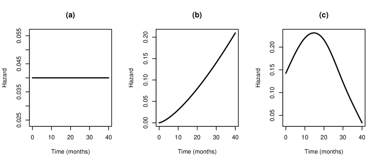
Figure 1: Assumed hazard functions for the (a) Exponential, (b) Weibull and (c) Super model.

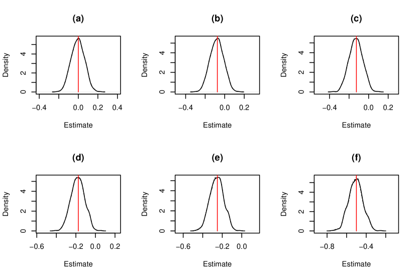
Figure 8: Distribution of posterior mean of the treatment effect from simulation estimation step when data are generated from the exponential proportional hazards model with (a) $\beta=0$, (b) $\beta=-0.075$, (c) $\beta=-0.125$, (d) $\beta=-0.175$, (e) $\beta=-0.25$, (f) $\beta=-0.5$ and the treatment effect was estimated based on the exponential ($\cdots$), general Bayesian ($-$) and Weibull ($-\leavevmode\nobreak\ -$) models.

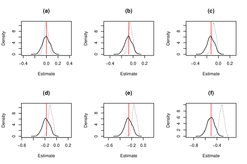
Figure 9: Distribution of posterior mean of the treatment effect from simulation estimation step when data are generated from the Weibull proportional hazards model with (a) $\beta=0$, (b) $\beta=-0.075$, (c) $\beta=-0.125$, (d) $\beta=-0.175$, (e) $\beta=-0.25$, (f) $\beta=-0.5$ and the treatment effect was estimated based on the exponential ($\cdots$), general Bayesian ($-$) and Weibull ($-\leavevmode\nobreak\ -$) models.

The distribution of the posterior means when the super model was generating data is shown in Figure 2. The corresponding plots for when the exponential and Weibull models were generating data are given in the appendix, see Figures 8 and 9, respectively. What is clear from these distributions is that biased estimates of the treatment effect can be observed. In particular, when the Weibull model is generating data, fitting the exponential model underestimates the treatment effect. Similarly, when the data were generated from the super model, fitting the exponential and Weibull models under and over estimates the treatment effect, respectively. In addition, this under/over estimation appears to become worse as the size of the effect of treatment increases. Overall, regardless of which model generated the data, the general Bayesian model appears to provide the least biased estimate of the treatment effect.

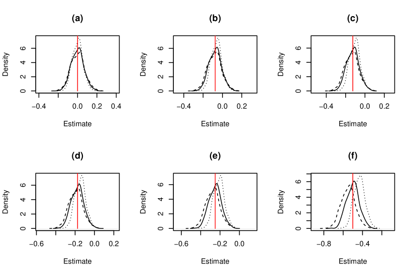
Figure 2: Distribution of posterior mean of the treatment effect from simulation estimation step when data are generated from the super model with (a) $\beta=0$, (b) $\beta=-0.075$, (c) $\beta=-0.125$, (d) $\beta=-0.175$, (e) $\beta=-0.25$, (f) $\beta=-0.5$ and the treatment effect was estimated based on the exponential ($\cdots$), general Bayesian ($-$) and Weibull ($-\leavevmode\nobreak\ -$) models.

6.2 Adaptive design under specific forms of the baseline hazard function

Next, we consider the above set up for the adaptive design of the ORVAC trial. Similar to the above approach, three models were considered for data generation, and the specific baseline hazard functions under each model are given in Figure 1. Again, the exponential, Weibull and general Bayesian models were then used to estimate the treatment effect and as the basis for evaluating the decision rules. To summarise each simulation, the posterior mean treatment effect was recorded along with the probability of stopping for effectiveness and futility. These summary statistics were recorded regardless of whether the maximum sample size was reached or the trial stopped early. In the latter case, the total number of enrolments was also recorded.

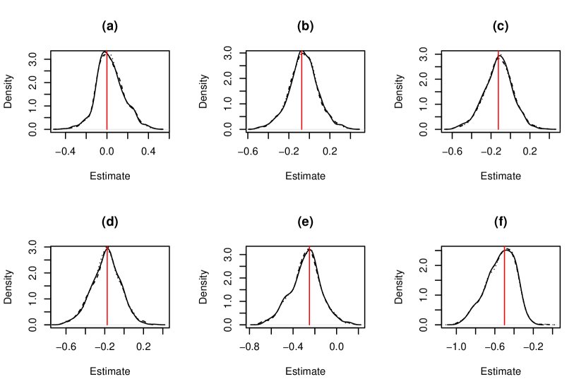
Figure 10: Distribution of posterior mean of the treatment effect from adaptive design when data are generated from the exponential model with (a) $\beta=0$, (b) $\beta=-0.075$, (c) $\beta=-0.125$, (d) $\beta=-0.175$, (e) $\beta=-0.25$, (f) $\beta=-0.5$ and the treatment effect was estimated based on the exponential ($\cdots$), general Bayesian ($-$) and Weibull ($-\leavevmode\nobreak\ -$) models.

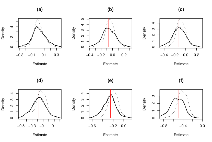
Figure 11: Distribution of posterior mean of the treatment effect from adaptive design when data are generated from the Weibull model with (a) $\beta=0$, (b) $\beta=-0.075$, (c) $\beta=-0.125$, (d) $\beta=-0.175$, (e) $\beta=-0.25$, (f) $\beta=-0.5$ and the treatment effect was estimated based on the exponential ($\cdots$), general Bayesian ($-$) and Weibull ($-\leavevmode\nobreak\ -$) models.

We start by inspecting the distribution of posterior means which is shown in Figure 3 for when the super model was generating data, and shown for the exponential and Weibull models in the appendix, see Figures 10 and 11, respectively. From the plots, it appears as though similar conclusions to the simulation and estimation step above can be drawn here. That is, when the data were generated from the super model, using the exponential or Weibull model results in under and over estimation of the treatment effect, respectively. This is particularly noticeable for the larger treatment effects. This is in contrast to the general Bayesian model which appears to provide relatively unbiased estimates of the treatment effect. When there is no treatment effect, the differences between the distributions appear to be minimal.

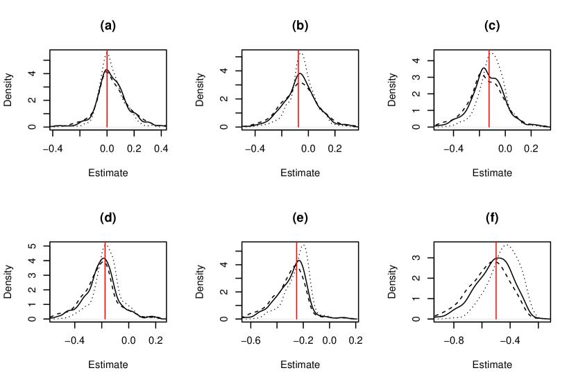
Figure 3: Distribution of posterior mean of the treatment effect from adaptive design when data are generated from the super model with (a) $\beta=0$, (b) $\beta=-0.075$, (c) $\beta=-0.125$, (d) $\beta=-0.175$, (e) $\beta=-0.25$, (f) $\beta=-0.5$ and the treatment effect was estimated based on the exponential ($\cdots$), general Bayesian ($-$) and Weibull ($-\leavevmode\nobreak\ -$) models.

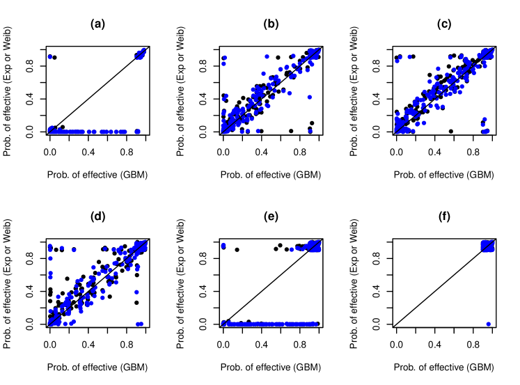
Figure 12: Effectiveness probability for each simulated trial when data were generated from the exponential model with (a) $\beta=0$, (b) $\beta=-0.075$, (c) $\beta=-0.125$, (d) $\beta=-0.175$, (e) $\beta=-0.25$ and (f) $\beta=-0.5$ and the treatment effect was estimated based on the general Bayesian, exponential (black) and Weibull (blue) models.

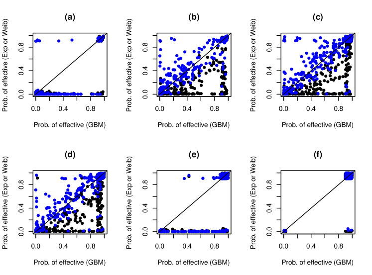
Figure 13: Effectiveness probability for each simulated trial when data were generated from the Weibull model with (a) $\beta=0$, (b) $\beta=-0.075$, (c) $\beta=-0.125$, (d) $\beta=-0.175$, (e) $\beta=-0.25$ and (f) $\beta=-0.5$ and the treatment effect was estimated based on the general Bayesian, exponential (black) and Weibull (blue) models.

At the end of each simulated trial, the probability of stopping for effectiveness was recorded. This is shown in Figure 4 when the super model was generating data with the corresponding plots for the exponential and Weibull models given in the appendix, see Figures 12 and 13, respectively. From Figure 4, it can be seen that fitting the exponential and the Weibull model results in under and over estimates of the probability of effectiveness (with respect to the general Bayesian model). This means that, in each case, one is more or less likely to stop the trial for this reason, depending on which model is adopted for inference. This effect may be seen in plots 4(a) and 4(e) where the general Bayesian model appears to have many probabilities between 0 and 1 while more certainty about stopping or not is given under the exponential and Weibull models. Of note, when the exponential or Weibull models are generating data, the probability of effectiveness under the general Bayesian model is generally consistent with what was given under the true data generating process. Overall, these results seem to align with those for estimating the treatment effect in that the exponential model under estimates the treatment effect which corresponds to generally lower probabilities of effectiveness. Similarly, the Weibull model over estimates the treatment effect which corresponds to generally higher probabilities of effectiveness.

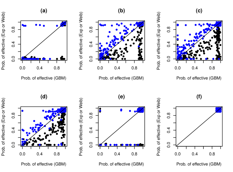
Figure 4: Effectiveness probability for each simulated trial when data were generated from the super model with (a) $\beta=0$, (b) $\beta=-0.075$, (c) $\beta=-0.125$, (d) $\beta=-0.175$, (e) $\beta=-0.25$ and (f) $\beta=-0.5$ and the treatment effect was estimated based on the general Bayesian, exponential (black) and Weibull (blue) models.

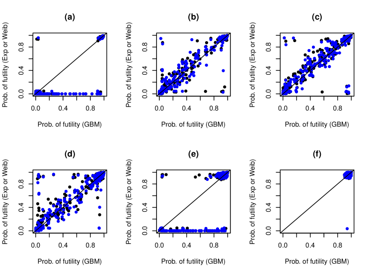
Figure 14: Futility probability for each simulated trial when data were generated from the exponential model with (a) $\beta=0$, (b) $\beta=-0.075$, (c) $\beta=-0.125$, (d) $\beta=-0.175$, (e) $\beta=-0.25$ and (f) $\beta=-0.5$ and the treatment effect was estimated based on the general Bayesian, exponential (black) and Weibull (blue) models.

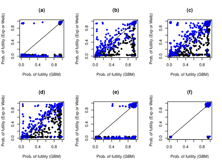
Figure 15: Futility probability for each simulated trial when data were generated from the Weibull model with (a) $\beta=0$, (b) $\beta=-0.075$, (c) $\beta=-0.125$, (d) $\beta=-0.175$, (e) $\beta=-0.25$ and (f) $\beta=-0.5$ and the treatment effect was estimated based on the general Bayesian, exponential (black) and Weibull (blue) models.

Figure 5 shows the probability of futility from each simulated trial when the super model was generating data, with the corresponding plots for the exponential and Weibull models given in the appendix, see Figures 14 and 15, respectively. From Figure 5, similar conclusions about the probability of declaring futility can be drawn as described above for declaring effectiveness. That is, the exponential and Weibull models tend to under and over estimate these probabilities (respectively) when compared to the general Bayesian model. Again, under the general Bayesian model, estimates of these probabilities are consistent with what was given under the true data generating model. Again, this aligns with the estimates of treatment effect as discussed above.

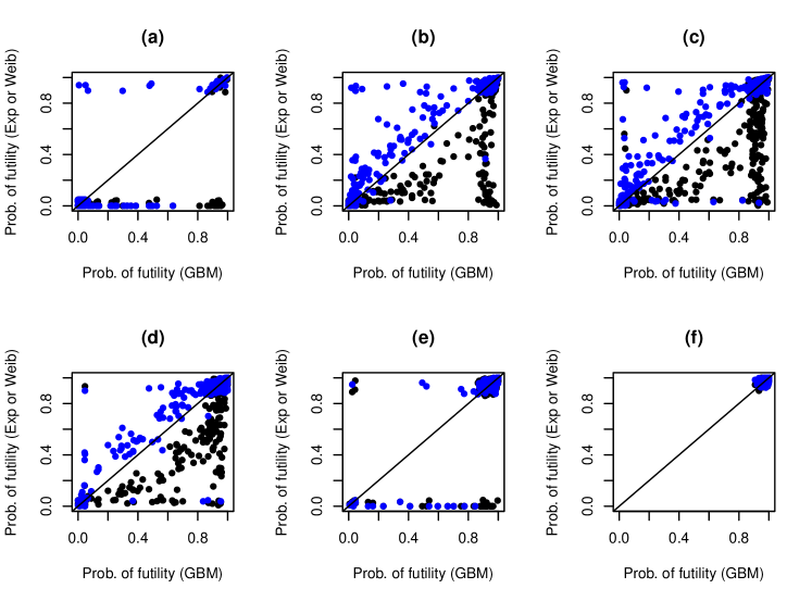
Figure 5: Futility probability for each simulated trial when data were generated from the super model with (a) $\beta=0$, (b) $\beta=-0.075$, (c) $\beta=-0.125$, (d) $\beta=-0.175$, (e) $\beta=-0.25$ and (f) $\beta=-0.5$ and the treatment effect was estimated based on the general Bayesian, exponential (black) and Weibull (blue) models.

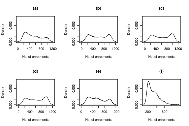
Figure 16: Total number of enrolments for each simulated trial when data were generated from the exponential model with (a) $\beta=0$, (b) $\beta=-0.075$, (c) $\beta=-0.125$, (d) $\beta=-0.175$, (e) $\beta=-0.25$ and (f) $\beta=-0.5$ and the treatment was estimated based on the exponential ($\cdots$), general Bayesian ($-$) and Weibull ($-\leavevmode\nobreak\ -$) models.

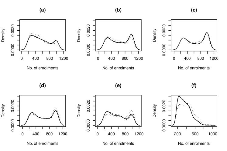
Figure 17: Total number of enrolments for each simulated trial when data were generated from the Weibull model with (a) $\beta=0$, (b) $\beta=-0.075$, (c) $\beta=-0.125$, (d) $\beta=-0.175$, (e) $\beta=-0.25$ and (f) $\beta=-0.5$ and the treatment was estimated based on the exponential ($\cdots$), general Bayesian ($-$) and Weibull ($-\leavevmode\nobreak\ -$) models.

Lastly, we assessed the total number of enrolments in each simulated trial. Figure 6 shows the total number of enrolments when the super model was generating the data, with the corresponding plots for the exponential and Weibull models given in the appendix, see Figures 16 and 17, respectively. From Figure 6, there is little difference in the number of enrolments between the three models when there is no effect of treatment. However, as the treatment effect increases, differences are revealed. In particular, the use of the exponential model appears to lead to, on average, more enrolments than using the general Bayesian and Weibull models. This is particularly noticeable when relatively moderately sized treatment effects are assumed as a larger number of trial simulations reach the maximum sample size. In terms of comparing the general Bayesian and Weibull models, the Weibull model appears to enroll slightly fewer participants highlighted by generally more trial simulations enrolling at or near the minimum sample size. When the exponential model was generating the data (see Figure 16), there is general agreement between the number of enrolments based on the three models used to estimate the treatment effect. This suggests that there is no noticeable efficiency losses associated with using an undefined baseline hazard function (as in the general Bayesian model). Similarly, when the Weibull models was generating the data, the number of enrolments between the general Bayesian and Weibull models agree. However, for the exponential model, the number of enrolments are generally higher when the treatment as an effect, and are generally lower when there is no effect of treatment.

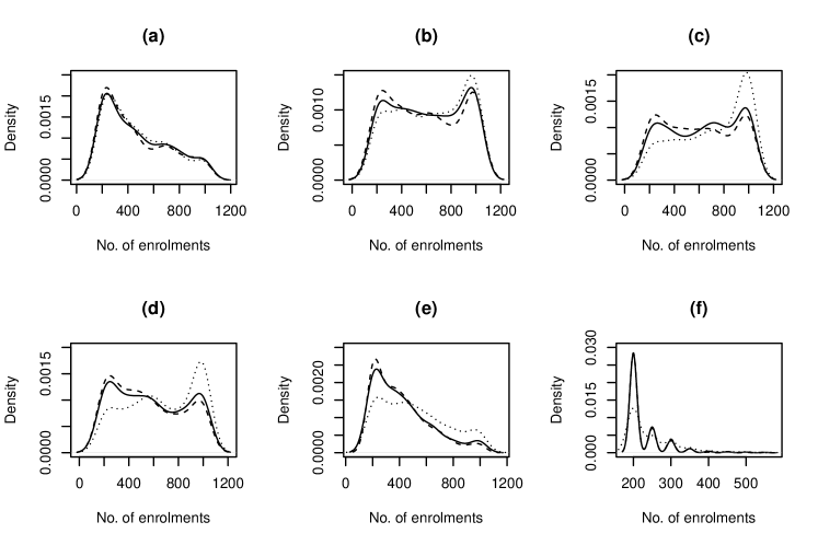
Figure 6: Total number of enrolments for each simulated trial when data were generated from the super model with (a) $\beta=0$, (b) $\beta=-0.075$, (c) $\beta=-0.125$, (d) $\beta=-0.175$, (e) $\beta=-0.25$ and (f) $\beta=-0.5$ and the treatment was estimated based on the exponential ($\cdots$), general Bayesian ($-$) and Weibull ($-\leavevmode\nobreak\ -$) models.

6.3 Adaptive design under a range of baseline hazard functions

Next we explore the performance of the three different models under a range of baseline hazards functions that could be observed under the super model. Specifically, for each simulation, we generated the treatment effect from a Uniform distribution i.e. $\beta\sim U(-0.75,-0.25)$, and each of the values corresponding to the knots (as described at the start of in Section 6), independently, from a Uniform distribution with lower and upper bounds of 0 and 0.4, respectively. To provide insight into the range of baseline hazards functions that could be observed when they are generated in this way, Figure 7(a) shows 10 realisations of the baseline hazard function under the super model. As can be seen, a range of functions can be observed with some being non-monotonic and others potentially being adequately described by an exponential or Weibull model i.e. some functions are relatively flat and some are monotonic.

A summary of the estimated treatment effects from this simulation study is provided in Figure 7(b) which shows the distribution of the difference between the true and estimated treatment effects (i.e. posterior modes) based on the exponential, Weibull and general Bayesian models. As can be seen, both the exponential and Weibull models provide slightly biased estimates of the treatment effect with a median difference of $0.0503$ and $-0.0607$, respectively. This agrees with the results above where the exponential model seems to underestimate the treatment effect while the Weibull model tends to overestimate it. In comparison, the general Bayesian model appears to provide a relatively unbiased estimate of the treatment effect with a median difference of $-0.0087$. Moreover, if we consider the median squared error, then the exponential, Weibull and general Bayesian models yield $0.0091$, $0.0084$ and $0.0100$, respectively, providing further support for the use of a general Bayesian model to design adaptive clinical trials. The third plot in Figure 7 shows the number of enrolments under the general Bayesian model compared to those under the exponential and Weibull models. As was observed previously, the use of the exponential model appears to result in, on average, a larger number of enrolments when compared to the general Bayesian model, with a mean difference of 18 enrolments. Similarly, the use of the Weibull model appears to lead to fewer participants being enrolled in the trials with a mean difference of $-$5.2. In terms of the observed probabilities of success and futility, no appreciable differences were observed, so summaries of these have been omitted.

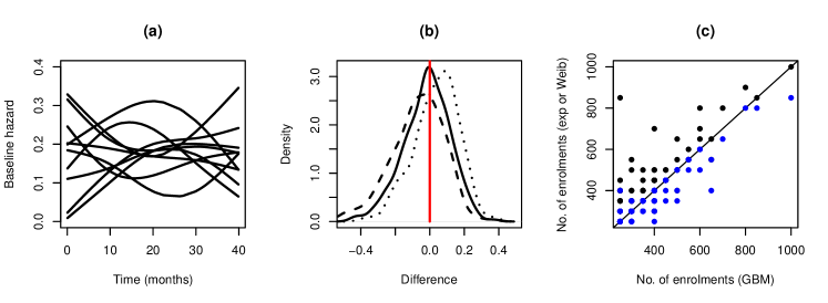
Figure 7: Adaptive design simulation where the super model was generating data where (a) shows 10 examples of realisations of the baseline hazard function; and (b) shows the distribution of the difference between the true and estimated treatment effect under the exponential ($\cdots$), general Bayesian ($-$) and Weibull ($-\leavevmode\nobreak\ -$) models, and (c) shows the number of enrolments under the general Bayesian model compared to the exponential (black) and Weibull (blue) models.

7 Discussion

We have proposed an approach to design adaptive clinical trials for time-to-event outcomes within a general Bayesian framework. The motivation for this was to reduce the number of assumptions about the data generating process that need to be made when designing these trials. Here, this related to removing the need to specify a specific form for the baseline hazard function with instead assuming it could have one of infinite forms based on a super model. Throughout this paper, we showed that such an approach was particularly useful as misspecifying the baseline hazard function could lead to biased estimates of the treatment effect, and also had implications for conducting the trial including potentially stopping too soon or running the trial for too long. In addition, it was observed that the number of enrolments under the general Bayesian model was similar to the exponential and Weibull models when they were generating the data. This suggests that estimating the treatment effect based on an undefined baseline hazard function did not result in any noticeable loss in estimation efficiency compared to adopting the true parametric form. Accordingly, we hope that the approach proposed in this paper can be used to design more robust and therefore more appropriate adaptive trials where time-to-event outcomes are observed.

While the benefits of our approach have been demonstrated, there are limitations of this work. We believe the main such limitation is the need to assume proportional hazards between treatment groups. While this is a common assumption, particularly when designing trials, we suggest that in practice such an assumption may not be appropriate, see, for example, [37]. Accordingly, we are interested in extending our proposed approach to relax this assumption, potentially by considering a flexible functional form for $\psi_{i}$, and undertaking inference within a general Bayesian framework. This is a research avenue we intend to explore into the future.

More generally, there is scope to extend our proposed approach to other data types including to overdispersed settings. In such cases, considering a quasi-likelihood [29] might be appropriate or an appropriate loss function could be developed, and a general Bayesian approach could be adopted for inference. An additional challenge of using such loss functions would be the need to calibrate $w$ in Equation (1), see [32]. Given this will need to be evaluated many times within trial simulation, computationally efficiency approaches are needed (e.g. [26]). Again, this is an area we plan to explore into the future.

Appendix A Prior information

Throughout this paper, vaguely informative prior information was considered when forming posterior distributions such that the results would be largely driven by the simulated data. Specifically, the following normal priors were considered:

• Exponential proportional hazards model: $(\log\lambda,\beta)\sim\mbox{MVN}[(\log 0.04,0),\mbox{diag}(5,10)]$

• Weibull proportional hazards model: $(\log\lambda,\log\gamma,\beta)\sim\mbox{MVN}[(\log 0.0005,\log 2.4,0),\mbox{diag}(5,5,10)]$

• Super model: $\beta\sim\mbox{N}[0,10]$,

where ‘N’ and ‘MVN’ denote the normal and multivariate normal distributions, respectively.

Appendix B Additional results

B.1 Distribution of posterior mean treatment effects from trial simulation

B.2 Distribution of posterior mean treatment effects from simulated trials

B.3 Probability of effectiveness from simulated trials

B.4 Probability of futility from simulated trials

B.5 Distribution of number of enrolments from simulated trials

References

- [1] J. S. Babb and A. Rogatko. Patient specific dosing in a cancer Phase I clinical trial. Statistics in Medicine, 20:2079–2090, 2001.
- [2] A. Bassi, J. Berkhof, D. de Jong, and P. M. van de Ven. Bayesian adaptive decision-theoretic designs for multi-arm multi-stage clinical trials. Statistical Methods in Medical Research, 30(3):717–730, 2021.
- [3] S. M. Berry, B. P. Carlin, J. Lee, and P. Muller. Bayesian adaptive methods for clinical trials. Chapman and Hall/CRC Biostatistics Series, Boca Raton, 2010.
- [4] P. Bissiri, C. Holmes, and S. Walker. A general framework for updating belief distributions. Journal of the Royal Statistical Society Series B, 78(5):1103–1130, 2016.
- [5] Y. Cheng and Y. Shen. Bayesian adaptive designs for clinical trials. Biometrics, 60:633–646, 2005.
- [6] S. C. Chow, M. Chang, and A. Pong. Statistical consideration of adaptive methods in clinical development. Journal of Biopharmaceutical Statistics, 15:575–591, 2005.
- [7] D. Collett. Modelling Survival Data in Medical Research. Chapman and Hall/CRC, Boca Raton, 3rd edition, 2015.
- [8] J. T. Connor, J. J. Elm, K. R. Brogliofor, and The ESETT and ADAPT-IT investigators. Bayesian adaptive trials for comparative effectiveness research: An example in status epilepticus. Journal of Clinical Epidemiology, 66:S130–S137, 2013.
- [9] D. R. Cox. Regression models and life-tables. Journal of the Royal Statistical Society Series B, 42:187–220, 1972.
- [10] D. R. Cox. Partial likelihood. Biometrika, 62:269–276, 1975.
- [11] D. R. Cox. A remark on censoring and surrogate response variables. Journal of the Royal Statistical Society Series B, 45:391–393, 1983.
- [12] A. Giovagnoli. The Bayesian design of adaptive clinical trials. International Journal of Environmental Research and Public Health, 18:530, 2021.
- [13] M. Girolami and B. Calderhead. Riemann manifold Langevin and Hamiltonian Monte Carlo methods. Journal of the Royal Statistical Society Series B, 73:123–214, 2011.
- [14] J. J. Harden and J. Kropko. Simulating duration data for the Cox model. Political Science Research and Methods, 7(4):921–928, 2019.
- [15] J. E. Herndon 2nd and F. E. Harrell Jr. The restricted cubic spline as baseline hazard in the proportional hazards model with step function time-dependent covariables. Statistics in Medicine, 14:2119–2129, 1995.
- [16] J. Hummel, S. Wang, and J. Kirkpatrick. Using simulation to optimize adaptive trial designs: applications in learning and confirmatory phase trials. Clinical Investigation, 5:401–413, 2015.
- [17] M. J. Jardine, S. S. Kotwal, A. Bassi, C. Hockham, M. Jones, A. Wilcox, C. Pollock, L. M. Burrell, J. McGree, V. Rathore, C. R. Jenkins, L. Gupta, A. Ritchie, A. Bangi, S. D’Cruz, A. J. McLachlan, S. Finfer, M. M. Cummins, T. Snelling, and V. Jha. Angiotensin receptor blockers for the treatment of COVID-19: pragmatic, adaptive, multicentre, phase 3, randomised controlled trial. BMJ, 379, 2022.
- [18] M. A. Jones, T. Graves, B. Middleton, J. Totterdell, T. Snelling, and J. A. Marsh. The ORVAC trial: a Phase IV, double-blind, randomised, placebo-controlled clinical trial of a third scheduled dose of Rotarix rotavirus vaccine in Australian Indigenous infants to improve protection against gastroenteritis: a statistical analysis plan. Trials, 21:741, 2020.
- [19] M. Kojima. Early completion of Phase I cancer clinical trials with Bayesian optimal interval design. Statistics in Medicine, 40:3215–3226, 2021.
- [20] R. Lewis and D. A. Berry. Group sequential clinical trials: A classical evaluation of Bayesian decision-theoretic designs. Journal of the American Statistical Association, 89:1528–1534, 1994.
- [21] J. M. McGree, C. Hockham, S. Kotwal, A. Wilcox, A. Bassi, C. Pollock, L. M. Burrell, T. Snelling, V. Jha, M. Jardine, and M. Jones. Controlled evaLuation of Angiotensin Receptor Blockers for COVID-19 respIraTorY disease (CLARITY): Statistical analysis plan for a randomised controlled Bayesian adaptive sample size trial. Trials, 23:361, 2022.
- [22] B. F. Middleton, M. A. Jones, C. S. Waddington, M. Danchin, C. McCallum, S. Gallagher, A. J. Leach, R. Andrews, C. Kirkwood, N. Cunliffe, J. Carapetis, J. A. Marsh, and T. Snelling. The ORVAC trial protocol: a phase IV, double-blind, randomised, placebo-controlled clinical trial of a third scheduled dose of Rotarix rotavirus vaccine in Australian Indigenous infants to improve protection against gastroenteritis. BMJ Open, 9(11), 2019.
- [23] B. North, H. M. Kocher, and P. Sasieni. A new pragmatic design for dose escalation in Phase I clinical trials using an adaptive continual reassessment method. BMC Cancer, 19:632, 2019.
- [24] A. O’Hagan. Bayes-Hermite quadrature. Journal of Statistical Planning and Inference, 29(3):245–260, 1991.
- [25] J. O’Quigley, M. Pepe, and L. Fisher. Continual reassessment method: a practical design for phase I clinical trials in cancer. Biometrics, 46:33–48, 1990.
- [26] A. M. Overstall and J. M. McGree. General Bayesian L2 calibration of mathematical models. https://arxiv.org/abs/2103.01132 [stat.ML], 2023.
- [27] A. M. Overstall, J. M. McGree, and C. C. Drovandi. An approach for finding fully Bayesian optimal designs using normal-based approximations to loss functions. Statistics and Computing, 28(2):343–358, 2018.
- [28] P. Pallmann, A. W. Bedding, B. Choodari-Oskooei, M. Dimairo, L. Flight, L. V. Hampson, J. Holmes, A. P. Mander, L. Odondi, M. R. Sydes, S. S. Villar, J. M. S. Wason, C. J. Weir, G. M. Wheeler, C. Yap, and T. Jaki. Adaptive designs in clinical trials: why use them, and how to run and report them. BMC Medicine, 16:29, 2018.
- [29] R. W. M. Wedderburn. Quasi-likelihood functions, generalised linear models, and the Gauss-Newton method. Biometrika, 61:439–447, 1974.
- [30] A. Schultz, J. A. Marsh, B. R. Saville, R. Norman, P. G. Middleton, H. W. Greville, S. M. Berry, and T. Snelling. Trial refresh: a case for an adaptive platform trial for pulmonary exacerbations of cystic fibrosis. Frontiers in Pharmacology, 10:301, 2019.
- [31] S. Senarathne, A. M. Overstall, and J. M. McGree. Bayesian adaptive n-of-1 trials for estimating population and individual treatment effects. Statistics in Medicine, 39:4499–4518, 2020.
- [32] N. Syring and R. Martin. Calibrating general posterior credible regions. Biometrika, 106(2):479–486, 12 2018.
- [33] P. Thall, L. Y. Inoue, and T. G. Martin. Adaptive decision making in a lymphocyte infusion trial. Biometrics, 58, 2002.
- [34] P. Thall, P. Mueller, Y. Xu, and M. Guindani. Bayesian nonparametric statistics: A new toolkit for discovery in cancer research. Pharmaceutical Statistics, 16:414–423, 2017.
- [35] P. Thall and R. Simon. A Bayesian approach to establishing sample size and monitoring criteria for Phase II clinical trials. Contemporary Clinical Trials, 15:463–481, 1994.
- [36] K. Thorlund, J. Haggstrom, J. J. H. Park, and E. J. Mills. Key design considerations for adaptive clinical trials: a primer for clinicians. BMJ, 360:k698, 2018.
- [37] Y. Wu, J. A. Marsh, E. S. McBryde, and T. L. Snelling. The influence of incomplete case ascertainment on measures of vaccine efficacy. Vaccine, 36(21):2946–2952, 2018.
- [38] Y. Xiao, Z. Liu, and F. Hu. Bayesian doubly adaptive randomization in clinical trials. Science China Mathematics, 60:2503–2514, 2017.
- [39] G. Yin and Y. Yuan. Bayesian dose finding in oncology for drug combinations by copula regression. Journal of the Royal Statistical Society Series C, 58:211–224, 2009.
- [40] Y. Yuan, X. Huang, and S. Liu. A Bayesian response-adaptive covariate-balanced randomization design with application to a leukemia clinical trial. Statistics in Medicine, 30:1218–1229, 2011.