Transmission-Guided Bayesian Generative Model for Smoke Segmentation

Abstract

Smoke segmentation is essential to precisely localize wildfire so that it can be extinguished in an early phase. Although deep neural networks have achieved promising results on image segmentation tasks, they are prone to be overconfident for smoke segmentation due to its non-rigid shape and transparent appearance. This is caused by both knowledge level uncertainty due to limited training data for accurate smoke segmentation and labeling level uncertainty representing the difficulty in labeling ground-truth. To effectively model the two types of uncertainty, we introduce a Bayesian generative model to simultaneously estimate the posterior distribution of model parameters and its predictions. Further, smoke images suffer from low contrast and ambiguity, inspired by physics-based image dehazing methods, we design a transmission-guided local coherence loss to guide the network to learn pair-wise relationships based on pixel distance and the transmission feature. To promote the development of this field, we also contribute a high-quality smoke segmentation dataset, SMOKE5K, consisting of 1,400 real and 4,000 synthetic images with pixel-wise annotation. Experimental results on benchmark testing datasets illustrate that our model achieves both accurate predictions and reliable uncertainty maps representing model ignorance about its prediction. Our code and dataset are publicly available at: https://github.com/redlessme/Transmission-BVM.

Introduction

Smoke segmentation (wildfire smoke in this paper) aims to localize the scope of the smoke area, and is usually defined as a binary segmentation task. Existing solutions (Xu et al. 2019; Yuan et al. 2021) mainly focus on effective feature aggregation with larger receptive fields for multi-scale prediction. We argue that, different from conventional binary segmentation tasks, i.e. salient object detection (Qin et al. 2019; Zhang et al. 2021a, c, b), background detection (Babaee, Dinh, and Rigoll 2017), and transparent object detection (Xie et al. 2020), smoke segmentation is unique from at least two perspectives: 1) the shape of smoke is non-rigid; thus structure-preserving solutions (Qin et al. 2019; Zhang et al. 2021a) adopted in existing binary segmentation models may not be effective; 2) smoke can be transparent, making it similar to transparent object detection. However, differently, models for transparent objects (Xie et al. 2020; He et al. 2021) focus on rigid objects, which makes smoke segmentation a more challenging task compared with existing binary segmentation or transparent object detection tasks.

To model smoke’s non-rigid shape and transparent appearance, we introduce a Bayesian generative model to estimate the posterior distribution of both model parameters and its predictions. Specifically, we introduce a Bayesian variational auto-encoder (Hu et al. 2019) to produce stochastic predictions, making it possible to capture uncertainty. Uncertainty (Der Kiureghian and Ditlevsen 2009; Kendall and Gal 2017) is defined as model ignorance about its prediction. (Der Kiureghian and Ditlevsen 2009) introduces two types of uncertainty, epistemic (model) uncertainty and aleatoric (data) uncertainty. The former is caused by ignorance about the task, which can be reduced with more training data. The latter is caused by labeling accuracy or ambiguity inherent in the labeling task, which usually cannot been reduced.

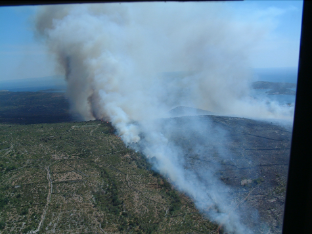
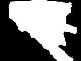
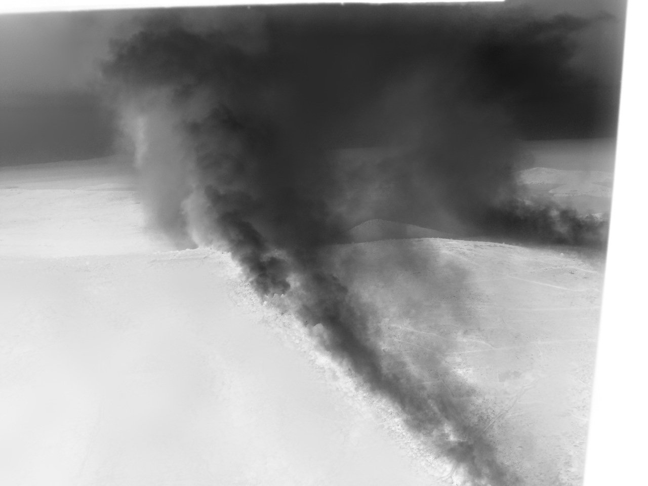
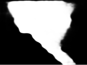
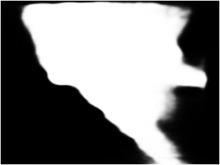
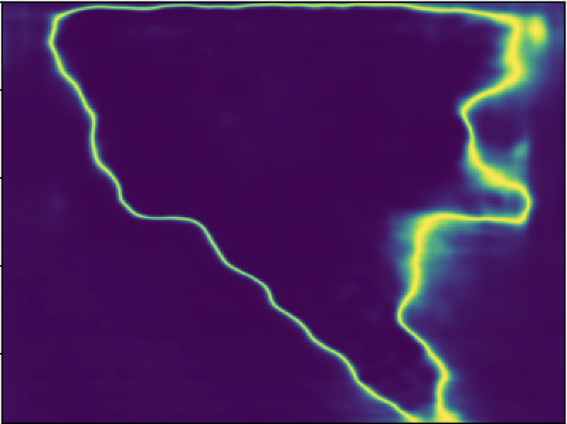
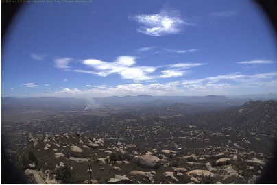
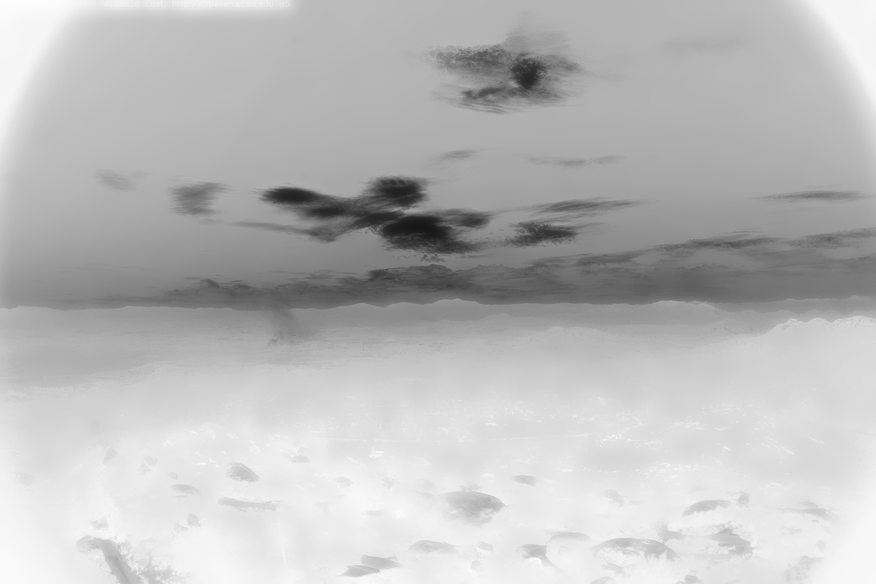
Image	GT	Trans.	w/o T	w/ T	Uncer.

Figure 1: Transmission loss is effective for segmenting smoke. From left to right: input images, ground-truth, transmission map, prediction without transmission loss, prediction with transmission loss, and predicted uncertainty. Row 1: modeling transmission features using our loss is helpful to distinguish the ambiguous boundary. Row 2: our transmission loss is effective with small smoke regions that have low contrast due to being semi-transparent.

For smoke segmentation, our limited knowledge about the smoke model leads to epistemic uncertainty, while the difficulty of labeling leads to aleatoric uncertainty. We intend to model both uncertainties within a Bayesian variational auto-encoder to achieve both accurate smoke segmentation and an estimation of a reliable uncertainty map representing model ignorance about its prediction given the training dataset and learned model parameters. Further, smoke images suffer from quality degradation, i.e. low contrast due to smoke’s translucent appearance, causing difficulty for classification. In the image enhancement field, (Li et al. 2021b; He, Sun, and Tang 2011) employ transmission that represents the portion of light that reaches the camera to model the quality degradation degree of images. In the smoke segmentation literature, (Miao, Chen, and Wang 2014; Shi, Lu, and Cui 2019a) exploit transmission to enhance the difference between smoke and background. Inspired by them, we propose a transmission-guided local coherence loss to model pair-wise similarity based on pixel distance and transmission to better differentiate smoke from background. We also employ reverse transmission as the weight of the loss to encourage the model to focus more on degraded regions.

We also find there exists no high-quality, large-scale smoke segmentation dataset. In Table 1, we compare benchmark smoke datasets in terms of size, image type, and annotation. The current largest real smoke dataset contains only 143 images. Although there is a large-scale synthetic image dataset SYN70K (Yuan et al. 2018), we find that the dataset is inadequate due to many redundant images. Furthermore, we notice that the widely used test sets for smoke segmentation are all synthetic. Due to the huge domain gap between the synthetic data and the real data, we claim that the model performs good on the synthetic data may not work well in real life. To promote the development of this field, we provide the first high-quality, large-scale smoke dataset with 5,000 training images and 400 testing images, where the training set consists of 1,400 real life images and 4,000 synthetic images with pixel-wise annotations, and the test images are all real life images. We also provide mask annotation and scribble annotation for fully supervised and weakly supervised smoke segmentation tasks.

We summarize our contributions as: 1) we introduce the first Bayesian generative model for smoke segmentation to produce both accurate predictions and reliable uncertainty maps given the non-rigid shape and transparent appearance of smoke; 2) we contribute a novel transmission loss to differentiate smoke from its background and encourage the model to emphasize the quality degraded regions. 3) we contribute a large-scale smoke segmentation dataset, containing 5,400 images with both pixel-wise mask and scribble annotations for effective model learning and evaluation.

Related Work

Smoke Segmentation: Existing methods rely on deep convolutional neural networks (CNNs), and mainly focus on: 1) multi-scale prediction (Long, Shelhamer, and Darrell 2014) as the size of the smoke varies in images; 2) high-low level feature aggregation for fusion (Lin et al. 2016b; Ding et al. 2018); and 3) enlarging the receptive field for effective context modeling (Chen et al. 2018; Yang et al. 2018). Among them, (Xu et al. 2019) designs a saliency detection network to highlight the most informative smoke with different levels of feature fusion. (Yuan et al. 2021) introduces a gated recurrent network with classification assistance resulting in further refinement. (Zhang et al. 2021d) proposes an Attention U-net to fuse coarse and fine layers for multi-scale prediction. (Li et al. 2020) relies on ASPP (Yang et al. 2018) to achieve large receptive fields. Different from current smoke segmentation methods that utilize generic semantic segmentation architectures and strategies, we tackle smoke segmentation based on smoke’s unique attributes, introducing uncertainty and transmission loss to model the non-rigid shape and translucent appearance.

Uncertainty Estimation: (Kendall and Gal 2017) defines two types of uncertainty: aleatoric and epistemic. Epistemic uncertainty is usually modeled by replacing model weights using a parametric distribution. Most solutions for epistemic uncertainty estimation are based on Bayesian neural networks (Neal 1996). As the posterior inference of model parameters is intractable, some works propose to use variational approximations to approximate the posterior inference, i.e.  Monte Carlo dropout (Gal and Ghahramani 2016), weight decay (Blundell et al. 2015), early stopping (Duvenaud, Maclaurin, and Adams 2016), ensemble models (Lakshminarayanan, Pritzel, and Blundell 2017), and M-head models (Rupprecht et al. 2017). Aleatoric uncertainty is usually obtained by generating a distribution over the model’s prediction space (Hu, Sclaroff, and Saenko 2020). (Kohl et al. 2018) proposes a UNet (Ronneberger, Fischer, and Brox 2015) with a conditional variational auto-encoder (Sohn, Lee, and Yan 2015) to capture labelling ambiguity. (Chang et al. 2020) uses stochastic embedding to capture the data uncertainty for classification. (Depeweg et al. 2018) defines the combination of the two types of uncertainty as predictive uncertainty to capture both epistemic uncertainty and aleatoric uncertainty simultaneously.

Dataset	Size	Type	Scribble	Mask
DST(2013)	740	Synthetic		✓
SSD(2018)	143	Real		✓
SYN70K(2018)	73632	Synthetic		✓
Ours	5400	Mixed	✓	✓

Table 1: Benchmark smoke segmentation datasets.

Medium Transmission: Medium transmission represents the portion of the light that reaches the camera, which is usually estimated using the dark channel prior algorithm (He, Sun, and Tang 2011). In image dehazing and enhancement (He, Sun, and Tang 2011; Li et al. 2016), transmission has been applied to emphasize degraded regions of the image. In smoke segmentation, (Miao, Chen, and Wang 2014) exploit transmission directly as a feature to detect smoke by thresholding the transmission map. Within the deep learning methods, (Shi, Lu, and Cui 2019b) performs smoke image classification by directly feeding the transmission map as input into a CNN to enhance the difference between smoke and background. To the best of our knowledge, although transmission has been explored in image enhancement, no previous deep learning based methods have investigated it for segmentation tasks. Different from existing solutions, we introduce a novel loss to model transmission similarity of pixels and encourage the model to focus on the degraded regions.

Smoke Segmentation Dataset: Currently, the largest smoke dataset is SYN70K (Yuan et al. 2018), a synthetic dataset consisting of a limited number of smoke objects in different scenes. Also, (Zhou et al. 2016) contributes a wildfire dataset with 2,192 real images captured by HPWREN cameras, but it does not contain mask annotation. To promote the field, we introduce the first high-quality, large-scale smoke segmentation dataset.

Our Method

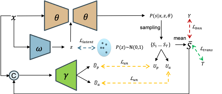
Figure 2: Overview of our Bayesian latent variable model for smoke segmentation, where ⓒ is the concatenation operation. To simplify the structure, we do not include the uncertainty calibration entropy loss here. The main modules included in our framework: a Bayesian Neural Network $P_{\theta}(y|x,z)$ to generate stochastic predictions, an inference model $P_{\omega}(z|x)$ to obtain the latent variable $z$, and the uncertainty estimation network $P_{\gamma}(x,P_{\theta}(y|x,z))$ to approximate the sampling based uncertainty for sampling-free uncertainty estimation during testing.

Our training dataset is $\mathcal{D}=\{(x_{i},y_{i})\}_{i=1}^{N}$, where $x_{i}$ is an input image, $y_{i}$ is the corresponding ground truth, and N is the size of the training dataset. Our proposed model consists of three sub-networks (see Fig. 2): 1) An inference network $P_{\omega}(z|x)$ with parameter set $\omega$ that encodes input $x_{i}$ into a low dimensional latent variable $z_{i}$, where the prior of $z_{i}$ is defined as a standard normal distribution $\mathcal{N}(0,1)$. The latent variable $z_{i}$ is used to capture the inherent noise in the input image that leads to the difficulty of labeling: aleatoric uncertainty. 2) A Bayesian network $P_{\theta}(y|x,z)$ maps input $x_{i}$ and generated latent variable $z_{i}$ to stochastic prediction $s_{i}=P_{\theta}(y|x_{i},z_{i})$, where model parameters $\theta$ are assumed to follow some specific distribution $P(\theta)$. 3) An uncertainty estimation network $g_{\gamma}$ that takes image pairs $(x_{i},s_{i})$ as input to approximate the sampling-based uncertainty produced by our Bayesian latent variable network, achieving sampling-free uncertainty estimation at test time, where $\gamma$ is the corresponding parameter set. Following (Depeweg et al. 2018), we use $g_{\gamma}$ to regress the total uncertainty and the aleatoric uncertainty, where the former is defined as the sum of aleatoric uncertainty and epistemic uncertainty.

Bayesian Latent Variable Model

Latent Variable Model: Smoke images are often corrupted by senor noise, and ambiguous due to smoke’s translucient appearance. Conventional deterministic networks based on the biased dataset can easily have over-confident predictions, leading to both high false-positive and false-negative rates. We argue that early detection of wildfires is critical to community safety, and a well-calibrated model is desirable.

Let us assume the noise-aware model prediction as:

$$y_{i}=f_{\theta}(x_{i},z_{i})+\epsilon_{i},$$ (1)

where $f_{\theta}(x_{i},z_{i})$ is the prediction of a neural network, $z_{i}$ is a latent variable, $\epsilon_{i}$ is additive noise drawn from a normal distribution $\mathcal{N}(0,\sigma^{2}\mathbb{I})$, with $\sigma$ as standard deviation. Given input $x_{i}$ and latent variable $z_{i}$, network output will be corrupted by additive noise $\epsilon_{i}$, which we assume is conditioned on the input image. It will lead the network to force $\sigma$ to be small to reduce the influence of the noise in the prediction. Then, the latent variable $z_{i}$ can capture unobserved stochastic features that can affect the network’s prediction.

Following conventional practice of variational auto-encoders, we train the latent variable by maximizing the expected variational lower bound (ELBO) as:

$$L(\theta,\omega;x) =\mathbb{E}_{z\sim{P_{\omega}(z|x)}}[-\log(P_{\theta}(y|x,z))]$$ (2)

$$+D_{KL}(P_{\omega}(z|x)||P(z)),$$

where $P_{\omega}(z|X)$ is the posterior distribution of the latent variable $z$ or the inference model, and $P(z)$ is its prior distribution, which we defined as a standard Gaussian distribution $\mathcal{N}(0,1)$. $D_{KL}(P_{\omega}(z|x)||P(z))$ is the Kullback-Leibler divergence regularizer. We design the inference model $P_{\omega}(z|X)$ with five convolutional layers that maps input $x$ into a low dimensional latent variable $z$ to capture the inherent ambiguities of human labeling. Specifically, the output of the inference model is $\mu^{post}$ and $\sigma^{post}$, leading to $P_{\omega}(z|x)=\mathcal{N}(\mu^{post},\sigma^{post})$ where $\mu^{post}$ and $\sigma^{post}$ represent the mean and the standard deviation of the posterior distribution of $z$, and $z$ is then obtained with the reparameteration trick: $z=\mu^{post}+\sigma^{post}*\epsilon$, where $\epsilon\sim\mathcal{N}(0,1)$.

Bayesian Neural Network with Latent Variable: Knowing when the model cannot be trusted is important in safety-critical systems such as wildfire detection. Bayesian neural networks (BNN) can model epistemic uncertainty by replacing the neural network’s weights with distributions. However, they suffer from huge computational burden due to the intractability of the posterior inference $P(\theta|D)$. Fortunately, BNNs can be approximated via variational inference with Monte Carlo (MC) dropout (Gal and Ghahramani 2016) by using Monte Carlo integration (Gal and Ghahramani 2016) to approximate the intractable marginal likelihood $P(y|x)$:

$$P(y|x,D)\approx\frac{1}{B}\sum_{b=1}^{B}P(y|x,\theta_{b}),$$ (3)

where $B$ indicates the times of sampling.

As $z$ can model the aleatoric uncertainty, and $P(\theta|D)$ can model epistemic uncertainty, with a Bayesian latent variable model, we aim to model both epistemic and aleatoric uncertainty, leading to predictive uncertainty estimation. We design our BNN based latent variable model (BNN-LVM) with a ResNet50 backbone (He et al. 2015) as encoder to obtain feature maps $\{f_{k}\}_{k=1}^{4}$ from different stages of the backbone. The latent variable $z$ is introduced to the network via two steps. Firstly, we sample $z$ from $P_{\omega}(z|x)$, and tile it to achieve the same spatial size as $f_{4}$. Secondly, we concatenate the tiled $z$ with $f_{4}$, and feed it to a $3\times 3$ convolutional layer to obtain $f_{4}^{\prime}$ of the same size as $f_{4}$, which will serve as the new backbone feature. To capture the epistemic uncertainty, the produced new features $\{\{f_{k}\}_{k=1}^{3},f_{4}^{\prime}\}$ are fed into four different $3\times 3$ convolutional layer with a dropout rate of 0.3 to get the new backbone features $\{s_{k}\}_{k=1}^{4}$. Subsequently, we use four residual channel attention modules (Fu et al. 2018) after each $s_{k}$ to obtain discriminative feature representations. Finally, we use a DenseASPP (Yang et al. 2018) module to aggregate higher-lower level features with enlarged receptive field and get the final prediction of our BNN-LVM as $s=P_{\theta}(y|x,z)$.

To train the BNN, we adopt the weighted structure-aware loss (Wei, Wang, and Huang 2019) as:

$$\mathcal{L}_{bnn}(s,y)=w*\mathcal{L}_{ce}(s,y)+\mathcal{L}_{iou}(s,y),$$ (4)

where $s$ and $y$ are the prediction and the ground truth respectively, $w$ is the edge-aware weight defined as $1+5*|H_{AP}(y)-y|$ where $H_{AP}$ is the average pooling function, $\mathcal{L}_{ce}$ and $\mathcal{L}_{iou}$ denote the cross-entropy loss and the IOU loss. $\mathcal{L}_{bnn}(s,y)$ is then the expected negative log likelihood term in Eq. 2.

Uncertainty Quantification: Uncertainty quantification (Jiawei Liu 2022; Li et al. 2021a; Zhang et al. 2021a) can provide more information about model prediction, leading to better decision making. For smoke segmentation, quantification of the uncertainty map can potentially reduce the false-alarm rate and guide people to resolve ambiguities.

Given the model prediction $P_{\theta}(y|x,z)$ from our BNN module, the predictive (total) uncertainty can be measured as entropy of the mean prediction, which can be formulated as $\mathcal{H}[\mathbb{E}_{P(\theta|D),z\sim P_{\omega}(z|x)}[P_{\theta}(y|x,z)]]$ where $\mathcal{H}$ denotes the entropy and $\mathbb{E}$ denotes the expectation. The corresponding expectation can be approximated by Monte Carlo (MC) integration, leading to mean prediction as:

$$p_{\mu}=\frac{1}{B}P_{\theta_{b}}(y|x,z),$$ (5)

where $B$ is the iterations of MC sampling, and $\theta_{b}$ is the parameter set of the $b^{th}$ iteration of sampling. The predictive uncertainty is then defined as: $U_{p}=\mathcal{H}[p_{\mu}]$. The aleatoric uncertainty is the average entropy for a fixed set of model weights, which can be formulated as: $U_{a}=\mathbb{E}_{P(\theta|D),z\sim P_{\omega}(z|x)}[\mathcal{H}[P_{\theta}(y|x,z)]]$. The epistemic uncertainty is then defined as the gap between predictive uncertainty and aleatoric uncertainty: $U_{e}=U_{p}-U_{a}$.

Uncertainty Estimation Network: Conventional solutions for uncertainty estimation involve multiple iterations of sampling (Jiawei Liu 2022; Zhang et al. 2020b) during testing, limiting the real-time application. As real-time performance is important for wildfire detection, we move the sampling process from the inference to the training stage. During training, we sample our BNN-LVN multiple times to obtain sampling-based predictive uncertainty and aleatoric uncertainty. Then, we use a designed uncertainty estimation network to approximate the calculated predictive uncertainty and aleatoric uncertainty. Specifically, our network produces two types of uncertainty with a widely used M-head structure (Rupprecht et al. 2017), where we use a shared encoder with five convolutional layers and two independent decoders with three convolutional layers to regress each type of uncertainty. The uncertainty estimation network $g_{\gamma}$ uses batch normalisation and LeakyReLU activation for all layers except the last layers of the two decoders. It takes the concatenation of image $x$ and its prediction $s$ as input to approximate the $U_{a}$ and $U_{b}$ by uncertainty consistency loss:

$$\mathcal{L}_{un}=\frac{1}{2}(\mathcal{L}_{mse}(U_{p},\hat{U_{p}})+\mathcal{L}_{mse}(U_{a},\hat{U_{a}})),$$ (6)

where $\mathcal{L}_{mse}$ is $L2$ distance, $\hat{U_{p}}$ and $\hat{U_{a}}$ are the approximated uncertainty maps with the proposed uncertainty estimation network $g_{\gamma}(x,s)$.

Transmission Guided Local Coherence Loss

With the loss function in Eq. 2 and the uncertainty estimation related loss in Eq. 6, we can already train our Bayesian latent variable model for smoke segmentation. However, we find that model with the smoke segmentation related loss in Eq. 4 fails to predict distinct boundaries at the ambiguous smoke edges. Inspired by image dehazing, we propose a transmission-guided local coherence loss, which exploits transmission as an essential feature to discriminate the smoke boundary. Our loss is based on the assumption that smoke objects tend to have a different transmission from most regions of the background. It can enforce similar predictions for pixels with similar transmission and close distance. Further, outdoor smoke images often suffer from quality degradation, i.e. low contrast. (Li et al. 2021b) shows that image quality degradation regions usually have lower transmission values. Inspired by (Li et al. 2021b), we use the reversed transmission value as the weight of our loss to encourage the model to focus on the degraded regions, which is defined as:

$$\mathcal{L}_{trans}=\sum_{m}\sum_{n\in K_{m}}(1-T(m))W(m,n)D(m,n),$$ (7)

where $K_{m}$ is a $k\times k$ kernel centered at pixel $m$, $D(m,n)$ is the $L1$ distance between the prediction of pixels $m$ and $n$, and $W(m,n)$ is a modified bilateral kernel in the form:

$$W(m,n)=\frac{1}{w}\exp(-\frac{||P(m)-P(n)||^{2}}{2\sigma_{P}^{2}}-\frac{||T(m)-T(n)||^{2}}{2\sigma^{2}_{T}}),$$ (8)

where $\frac{1}{w}$ is the normalized weight term, $P(m),P(n)$, and $T(m),T(n)$ represent the spatial information and transmission information of the pixels $m$ and $n$ respectively, and $\sigma_{P}^{2},\sigma_{T}^{2}$ are the kernel bandwidth.

To estimate medium transmission, we calculate transmission information of each pixel of the intensity image by:

$$T(m)=1-\min\limits_{c}(\min\limits_{n\in K(m)}(\frac{I^{c}(n)}{A^{c}})),$$ (9)

where $A$ is global atmospheric light, $I$ is the intensity image, $c$ is the color channel, $K(m)$ is a local patch of size $k\times k$ centered at pixel $m$ and then $\min\limits_{c}(\min\limits_{n\in K(m)}(\frac{I^{c}(n)}{A^{c}})$ is the normalized haze map defined at (He, Sun, and Tang 2011). We can see the estimated medium transmission is based on the global atmospheric light $A$. To get $A$, we follow (He, Sun, and Tang 2011) and obtain it by picking the top 0.1% brightest pixels in the dark channel of the intensity image.

Objective Function

So far, we have $\mathcal{L}(\theta,\omega;x)$ in Eq. 2 for the Bayesian latent variable model, $\mathcal{L}_{un}$ in Eq. 6 for the uncertainty estimation module, and $\mathcal{L}_{trans}$ in Eq. 7 to force the network focus on the image degradation regions. We further adapt entropy loss as a regularizer to encourage the prediction to be binary. Entropy loss is defined as the entropy of model prediction, which is minimized when the model produces binary predictions. However, we find that directly applying entropy loss to our task leads to overconfident predictions, causing extra false positives. To reduce the “binarization regularizer” for less confident regions, we add a temperature scaling term (Guo et al. 2017) to the original entropy loss, which uses learned total uncertainty as the temperature so that the model can produce softened predictions on high uncertainty pixels. Note that the temperature in our method is learned by the uncertainty estimation network rather than being a user-defined temperature as used in traditional temperature scaling methods. Our uncertainty-based temperature scaling can also be used to calibrate our model. A well-calibrated model cannot only reduce the gap between prediction confidence and model accuracy but also achieve better performance.

Our uncertainty calibrated entropy loss is defined as:

$$\mathcal{L}_{c}=-\sum_{c\in{0,1}}\sigma(s/U_{p})\log\sigma(s/U_{p}),$$ (10)

where $\sigma$ is the sigmoid function, $s$ is the network prediction, and $U_{p}$ is the total uncertainty.

Finally, our total loss for BNN-LVM is defined as:

$$\mathcal{L}_{gen}=\mathcal{L}(\theta,\omega;x)+\lambda_{1}\mathcal{L}_{trans}+\lambda_{2}\mathcal{L}_{c},$$ (11)

and empirically we set $\lambda_{1}=0.3$ and $\lambda_{2}=0.01$. With Eq. 11 we can update our Bayesian latent variable model, and the uncertainty estimation model $g_{\gamma}$ is updated with loss function $\mathcal{L}_{un}$ in Eq. 6.

Dataset	SMD	LRN	Deeplab v1	HG-Net8	LKM	RefineNet	PSPNet	CCL	DFN	DSS	W-Net	CGRNet	Ours
	(2018)	(2017)	(2018)	(2016)	(2017)	(2016b)	(2016)	(2018)	(2018)	(2018)	(2020)	(2021)
DS01	.3209	.3069	.2981	.3187	.2658	.2486	.2366	.2349	.2269	.2745	.2688	.2138	.1210
DS02	.3379	.3078	.3030	.3301	.2799	.2590	.2480	.2498	.2411	.2894	.2548	.2280	.1362
DS03	.3255	.3041	.3010	.3215	.2748	.2515	.2430	.2429	.2332	.2861	.2596	.2212	.1291

Table 2: Performance ($mMse\downarrow$) on three synthetic datasets.

SMOKE5K Dataset

As shown in Table 1, the existing largest real smoke segmentation dataset contains only 143 images. Although Yuan et al. create a large synthetic dataset for benchmarking, their dataset suffers from redundancy, as they crop and copy a limited number of simulated smoke to different scenes. To promote the development of the smoke segmentation, we create a high-quality smoke segmentation dataset, namely SMOKE5K, that consists of both synthetic images and real images for new benchmarking.

Dataset Construction

We create our dataset based on an open wildfire smoke dataset (Zhou et al. 2016), the current largest synthetic smoke dataset (Yuan et al. 2018) and a few images from the internet. Due to the large redundancy of the synthetic dataset, we only choose 4,000 images from the synthetic dataset and discard images that contain duplicated smoke foreground. For real datasets, we choose 1,360 good quality smoke images from the (Zhou et al. 2016) dataset, and discard smoke images of poor quality, and we also choose 40 smoke images from the internet to further increase the diversity of the test set. As the real smoke datasets do not have pixel-wise annotations, we then annotate the dataset with both binary mask and scribble annotation. Finally, we end up with 5,400 images, where 400 real smoke images from it is used for testing, which is defined as “Total”, and the remaining 5,000 images are for training. To better explore the difficulty of different attributes in the smoke segmentation models, we further extract 100 images from the 400 test images, denoted as “Difficult”, which mainly contains transparent smoke and smoke with more diverse shapes.

Dataset Comparison

We have carried out two experiments to verify the superiority of our dataset. Firstly, we train the same segmentation model on both SYN70K and our dataset SMOKE5K. It takes about three days to train on SYN70K and about 12 hours to train on our dataset. Then, we evaluate the two models on three synthetic datasets (DS01, DS02, DS03) from (Yuan et al. 2018), and the results are shown in Fig. 3 (a). We observe that although SYN70k is at least 14 times larger than our dataset, the model trained with our dataset still produces the lower mean square error (MSE) on all three synthetic test sets. Further, we evaluate the two models on our real image test set, and the result is shown in Fig. 3 (b), which further explains the effectiveness of our new training dataset.

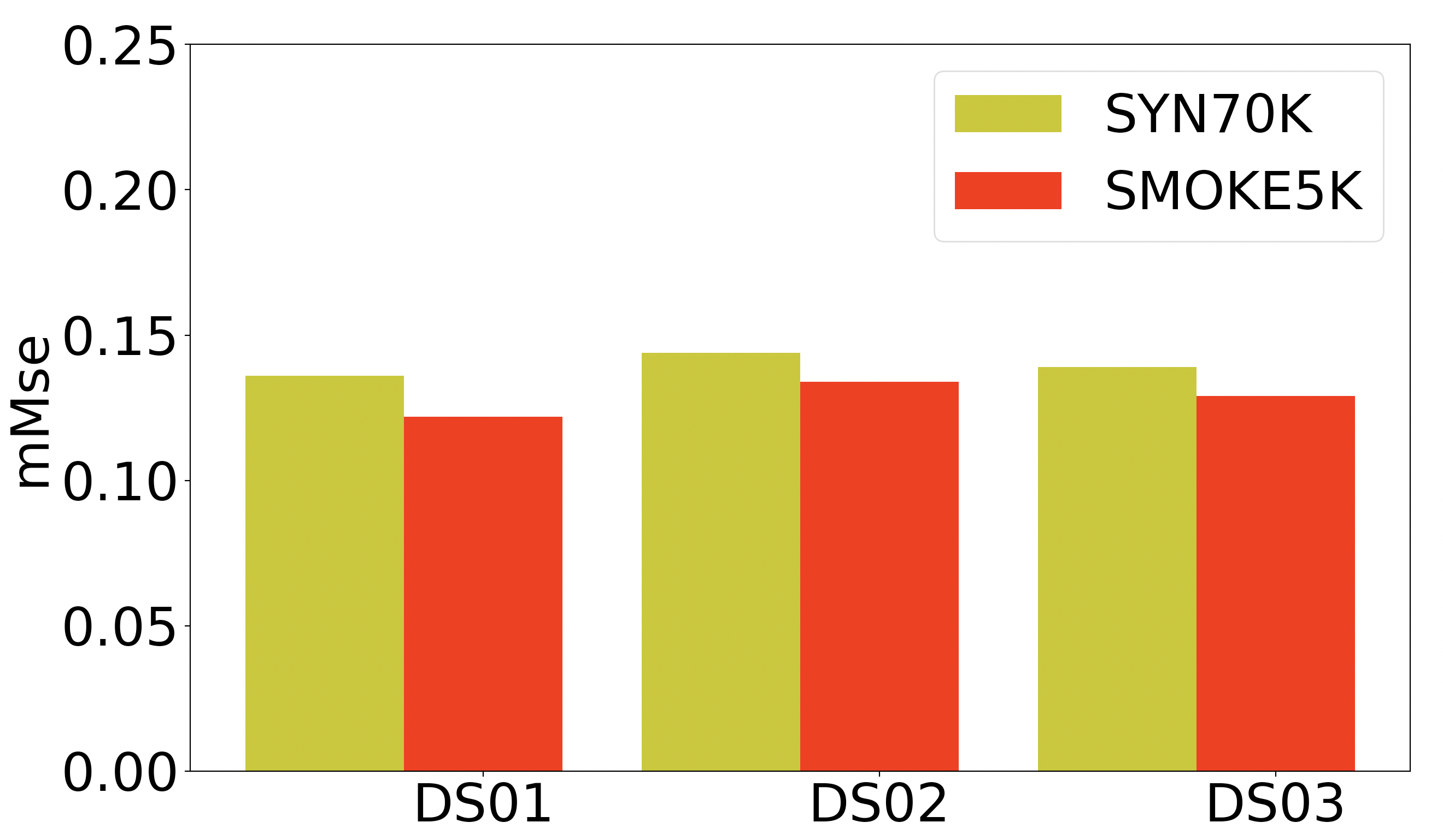
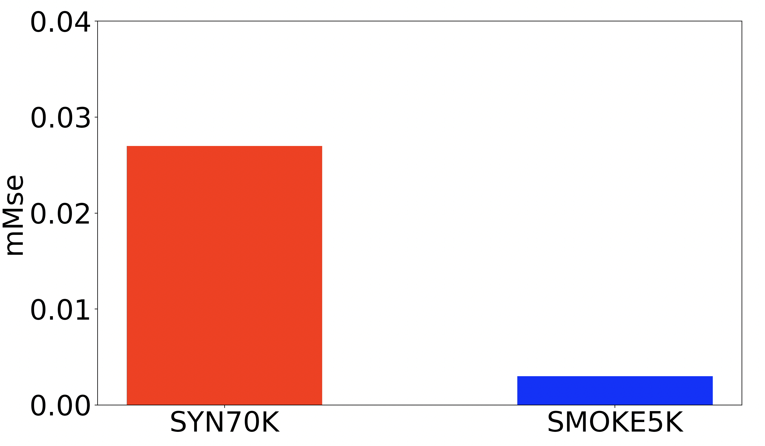
a	b

Figure 3: (a) Comparing the model trained using SYN70K and the model trained using SMOKE5K on the synthetic test set. (b) Comparing the model trained using SYN70K and the model trained using SMOKE5K on our real smoke dataset.

	Metric	F3Net	BASNet	SCRN	ITSD	UCNet	Ours
		(2019)	(2019)	(2019)	(2020)	(2021a)
T	$\mathcal{M}\downarrow$	.004	.005	.003	.003	.003	.002
	$F_{\beta}\uparrow$	.670	.733	.769	.774	.787	.791
D	$\mathcal{M}\downarrow$	.011	.014	.009	.010	.009	.006
	$F_{\beta}\uparrow$	.633	.662	.682	.688	.707	.741

Table 3: Performance on the test set of SMOKE5K.

Experimental Results

Implementation Details

Datasets: For fair comparisons with existing smoke segmentation models, we first follow the same settings in (Yuan et al. 2018) and train our model using SYN70K (Yuan et al. 2018) and evaluate on their three public smoke segmentation benchmarks: (1) DS01; (2) DS02; (3) DS03. Then, we provide a new benchmark by training with our SMOKE5K dataset and tests on our real-image testing set.

Baselines and Evaluation Metrics: We compare with existing smoke segmentation models following the first setting (training and testing on synthetic datasets) and report performance in Table 2. As no code is available for existing smoke segmentation models, we select five state-of-the-art saliency detection baselines (F3Net (Wei, Wang, and Huang 2019), BASNet (Qin et al. 2019), SCRN (Wu, Su, and Huang 2019), ITSD (Zhou et al. 2020) and UCNet (Zhang et al. 2021a)) due to the similarity between the two tasks. We re-train them on our new smoke segmentation benchmark, the SMOKE5K dataset. We show the results in Table 3.

Following previous smoke segmentation literature, we choose the Mean Square Error (Mse) ($\mathcal{M}$) as the evaluation metric. The average Mses (mMse) on the test set is used to measure performance. Mse computes the per-pixel accuracy of model prediction, which depends on the size of the smoke foreground, leading to inherent small Mse for smoke image with small size of smoke. To tackle the problem, we adopt the F-measure ($F_{\beta}$) as complementary to mMse for comprehensive performance evaluation, which is a weighted combination of precision and recall values. Further, as an uncertainty estimation model, we also adopt the reliability diagram (Guo et al. 2017) and dense calibration measure (ECE) (Zhang et al. 2020a) to represent model’s calibration degree.

Training Details: We train our framework using PyTorch with a maximum of 50 epochs. Each image is re-scaled to $480\times 480$. Empirically, we set the dimension of the latent space $z$ as 8. The learning rates of the generator $P_{\theta}(y|x,z)$ and the uncertainty estimation network $g_{\gamma}$ are initialized to 2.5e-5 and 1.5e-5, respectively. We use the Adam optimizer and decrease the learning rate 0.8 after 40 epochs with a maximum epoch of 50. We adopt ResNet50 backbone to the encoder of $P_{\theta}(y|x,z)$, which is initialized with parameters trained for image classification, and the other newly added layers are initialized with the PyTorch default initialization strategy. It took about three days of training on SYN70K and 15 hours on SMOKE5K with batch size 6 using a single NVIDIA GeForce RTX 2080Ti GPU.

Comparison with State-of-the-Art Methods

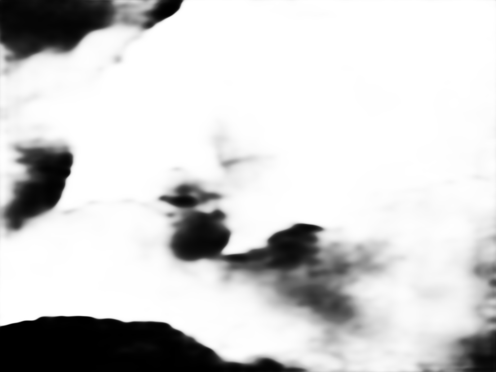
Image	GT	ITSD	UCNet	Ours

Figure 4: Qualitative comparison of predictions by our model and other state-of-the-other models.

Quantitative Comparison: In Table 2, we compare our model with the state-of-the-art methods by training and testing on the synthetic dataset (Yuan et al. 2018), and the significant performance improvement of our model validates effectiveness of our solution. We also provide a new benchmark of state-of-the-art models trained and tested on our SMOKE5K dataset, shown in Table 3. We retrain all models on our training set with their original setting. For the “Total (T)” test set, our model outperforms F3Net (Wei, Wang, and Huang 2019), BASNet (Qin et al. 2019), SCRN (Wu, Su, and Huang 2019), and ITSD (Zhou et al. 2020), and slightly outperforms UCNet (Zhang et al. 2021a). For the “Difficult (D)” test set, the consistently better performance against all state-of-the-art models demonstrates the effectiveness of our model for smoke segmentation.

Qualitative Comparison on SMOKE5K Dataset: We also visualize the predictions of our model and compared models, namely ITSD (Zhou et al. 2020) and UCNet (Zhang et al. 2021a) (the two best models in Table 3) in Fig. 4. In the first row, we find our prediction more complete and precise for the transparent part of the smoke that fills much of the image. In the second and third rows, we find that our model also performs better for small size of smoke.

Uncertainty Decomposition

In Fig. 5, we choose three representative images according to the difficulty to segment, denoted as simple, normal and difficult examples. We visualize our model predictions with the corresponding three types of uncertainties, namely “Aleatoric”, “Epistemic” and “Total” uncertainty. For the simple example (the first row), epistemic and aleatoric uncertainty capture similar patterns. For the medium example (the second row), epistemic uncertainty is increased on the translucent region of the smoke, which accounts for the out-of-distribution example of our training sets. For the difficult example (the third row), epistemic uncertainty is especially increased in fog regions. Further, we can see the total uncertainty captures both aleatoric uncertainty and epistemic uncertainty. In summary, we find that it is important to model aleatoric uncertainty for: (1) modeling ambiguity in annotations, and (2) modeling the non-rigid shape of objects. Further, it is important to model epistemic uncertainty for: (1) safety-critical applications, identifying out-of-distribution samples; and (2) the false-positive problems, where the epistemic uncertainty is usually increased in false-positive regions. The total uncertainty in general can provide more information about model prediction, leading to explainable and well-calibrated models.

Ablation Study

We perform the following experiments to analyze each component of our model. All experiments are evaluated on the test set of SMOKE5K. To evaluate the effectiveness of our method, we set our baseline by removing the transmission loss and the uncertainty calibration entropy loss, which is shown as “1” in Table 4. Note that it means our baseline does not exploit estimated uncertainty. Then, we combine the transmission loss and uncertainty calibration entropy loss gradually, denoted in “2” and “4” in Table 4.

		Base.	$\mathcal{L}_{trans}$	$\mathcal{L}_{en}$	$\mathcal{L}_{c}$	$\mathcal{M}\downarrow$	$F_{\beta}\uparrow$
T	1	✓				.005	.712
	2	✓	✓			.004	.741
	3	✓	✓	✓		.006	.695
	4	✓	✓		✓	.002	.791
D	1	✓				.014	.646
	2	✓	✓			.008	.714
	3	✓	✓	✓		.007	.726
	4	✓	✓		✓	.006	.741

Table 4: Ablation study for transmission loss, entropy loss and uncertainty calibration mechanism.

Impact of the Transmission Loss: We perform this ablation study by adding transmission loss to our baseline, shown as “2” in Table 4. Compared with baseline, we find transmission loss helps the model achieve a performance improvement on both “Total” and “Difficult” test sets. The greater improvement on the “Difficult” test set demonstrates our loss is useful for dealing with smoke’s transparent appearance. Further, in Fig. 1, it can be seen that the model with transmission loss (“w/T”) can better recognize ambiguous regions and deal with low contrast than the model without the transmission loss (“w/o T”), which demonstrates the effectiveness of the proposed transmission loss.

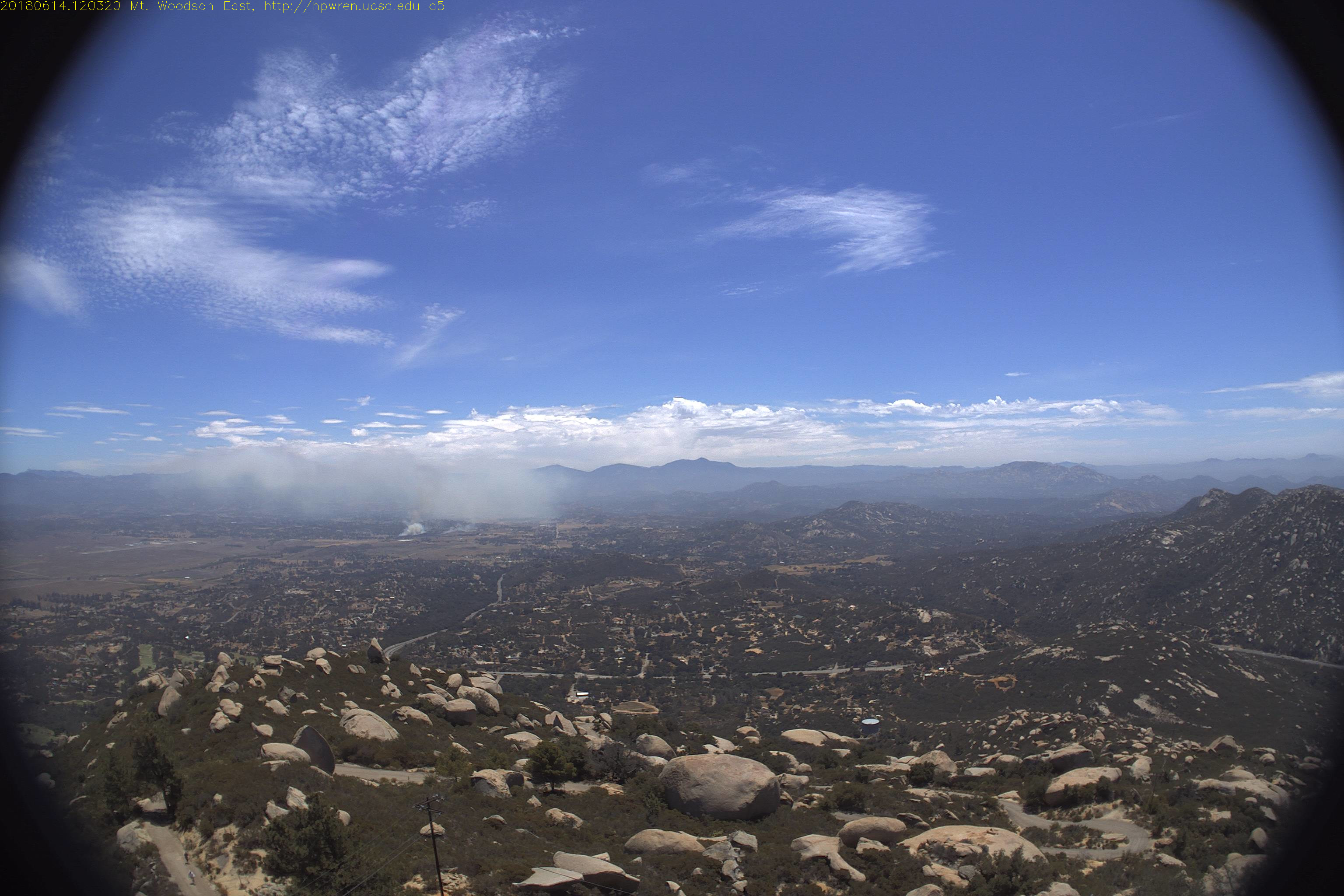
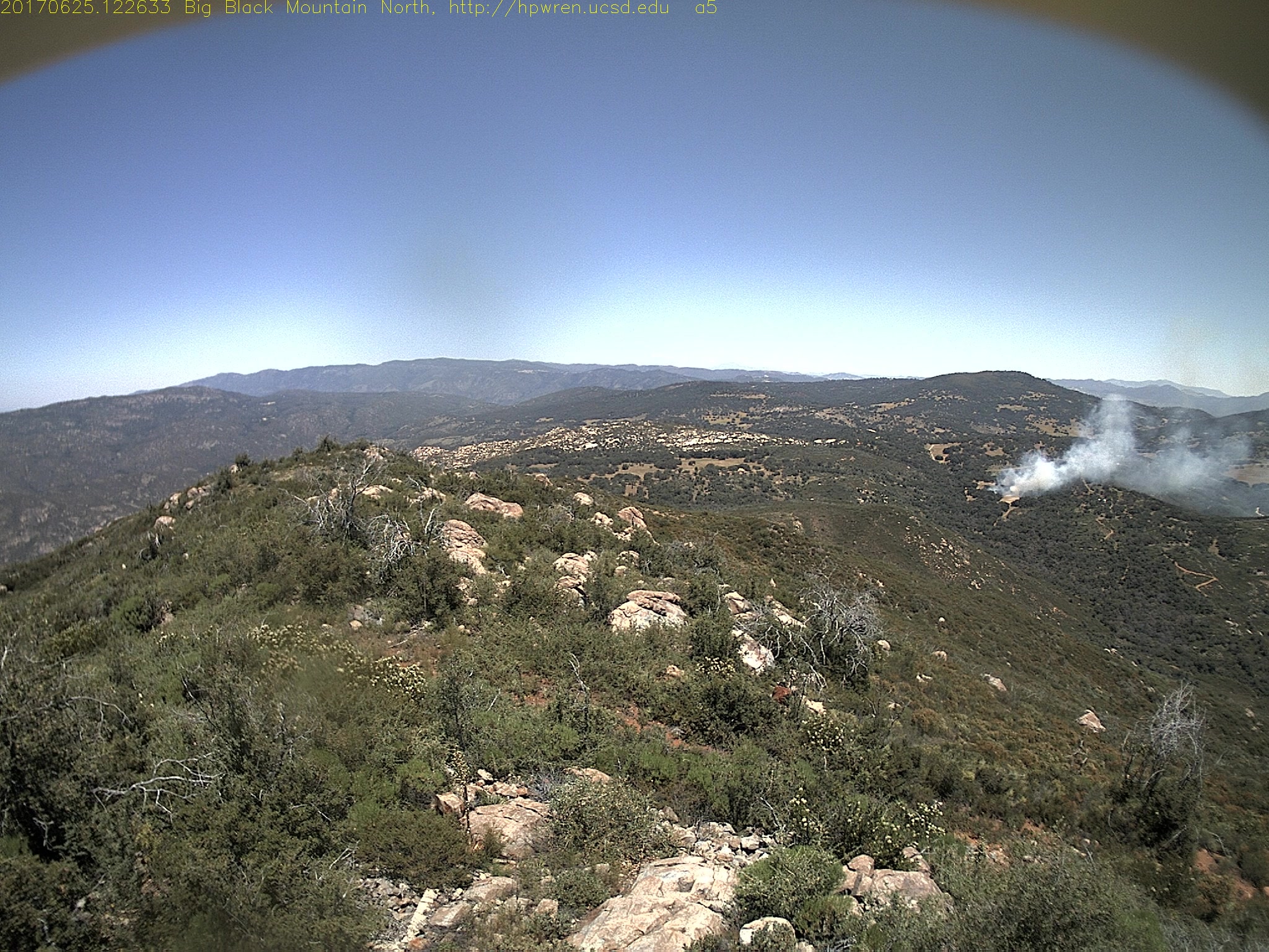
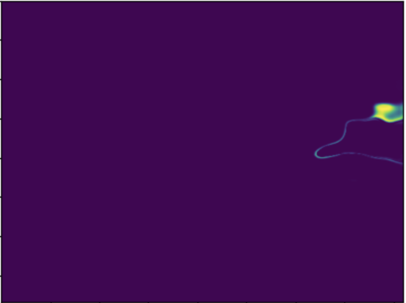
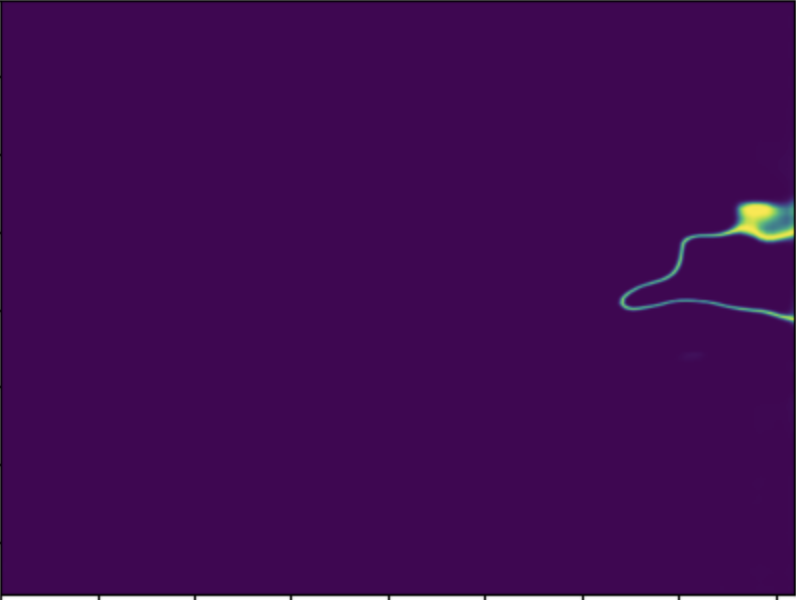
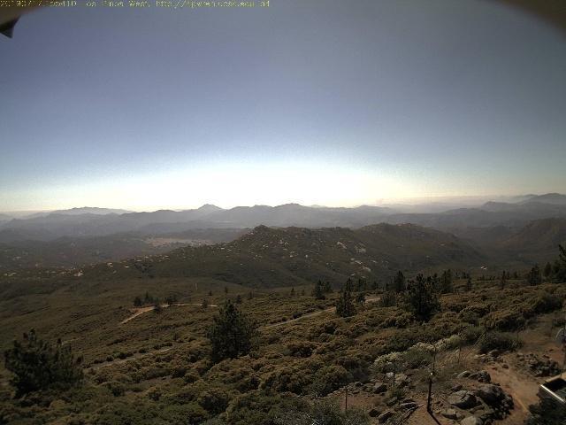
Img	GT	Pred	Aleatoric	Epistemic	Total

Figure 5: Visualisation of three kinds of uncertainty captured by our model (Please zoom in to see the uncertainty map). From top to bottom row: Simple example, normal example, difficult example.

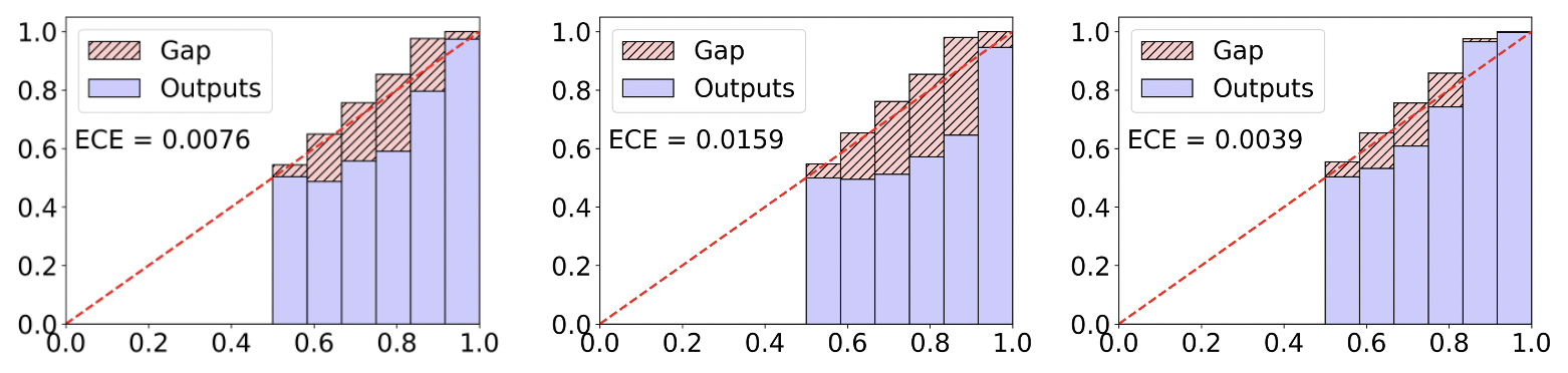
Figure 6: Reliability diagrams for UCNet (the $1^{st}$), our model before calibration (the $2^{nd}$), and our model after calibration (the $3^{rd}$). The horizontal axis of the reliability diagram denotes confidence, and the vertical axis denotes the accuracy.

Impact of Uncertainty Calibration: In this ablation study, we set our baseline as our model with transmission loss (“2” in Table 4). Based on it, we introduce entropy loss $\mathcal{L}_{en}$ to it to validate the uncertainty calibration entropy loss, and denote this experiment as “3” in Table 4. We can see that the performance for the “Total” test set is worse when we directly add entropy loss. The reason is that although entropy loss can encourage predictions to be binary, it will make predictions to be over-confident, and this negative influence will be significant for our “Total” test set as most smoke regions are very small. Then, we add uncertainty-based temperature scaling into entropy loss as in Eq. 10. We can see that the performance in all metrics is higher than the previous two models, which clearly shows the advantage of the proposed uncertainty calibration loss $\mathcal{L}_{c}$ in Eq. 10.

Further, as an uncertainty-aware learning method, we aim to achieve well calibrated model where model accuracy is consistent with model confidence. To measure the calibration quality, we follow the calibration definition in (Guo et al. 2017), and report the reliability diagrams in Fig. 6. We show the reliability diagrams of our model without calibration (setting 2 in Table 4) and our model after calibration (setting 4 in Table 4) in the second and third diagrams of Fig. 6, respectively. We also show reliability diagrams of UCNet (Zhang et al. 2021a) (another uncertainty estimation method using CVAEs (Sohn, Lee, and Yan 2015) for saliency detection) in the first diagram of Fig. 6. It can be seen that the gap between accuracy and confidence for UCNet is smaller than our model without calibration, leading to the ECE of 0.0076, but the calibration quality is still very low. With our uncertainty calibration entropy loss, the gap between confidence and accuracy for our model is significantly reduced, the dense calibration measure (ECE) is also reduced from 0.0159 to 0.0039, leading to a better calibrated model.

Conclusion

In this paper, we propose a Bayesian generative model to perform smoke segmentation and quantify the corresponding informative uncertainties. We also explore the medium transmission feature and propose a novel transmission loss to tackle smoke’s ambiguous boundary and low contrast problems. Further, we release the first high-quality, large-scale smoke segmentation dataset to promote the development of this field. Experiments on all benchmark test sets demonstrate the effectiveness of the proposed method, leading to both an accurate smoke segmentation model and reliable uncertainty maps indicating model’s confidence towards it’s prediction.

Overview

In this supplementary material, we provide more details about our dataset, evaluation metrics, qualitative comparisons, dark channel prior algorithm, and some discussions about model details.

Evaluation Metrics

Mean Square Error: $\mathcal{M}$ is defined as the per-pixel square difference between the prediction $s$ and the ground truth $y$. The average Mse ($mMse$) is usually used to evaluate model performance on test set, which is in the form of:

$$mMse=\frac{1}{N}\sum_{i=1}^{w}\sum_{j=1}^{h}(s_{ij}-y_{ij})^{2}$$ (12)

where N is the number of pixels in the image, $w$ and $h$ are the width and height of the image, $s$ and $y$ are the prediction and ground truth.

F-measure: F-measure combines both precision and recall to capture both properties, which is calculated based on each pair of precision and recall as:

$$F_{\beta}=\frac{(1+\beta^{2})\cdot precision\cdot recall}{\beta^{2}\cdot precision+recall}$$ (13)

where $\beta^{2}$ is set to 0.3 to assign more weight to precision.

Dense Calibration Measure: $\mathcal{M}$ and $F_{\beta}$ only evaluate the model accuracy but ignore the gap between model accuracy and its confidence, which cannot evaluate how the model is calibrated in a dataset. The dense calibration measure is an extension of (Guo et al. 2017), which is the weighted average of the difference between every bin’s accuracy and confidence. For each image $x_{i}$, the prediction $y_{i}$ is grouped into M interval bins, the dense calibration error is then defined as:

$$ECE^{i}=\sum_{m=1}^{M}\frac{|B_{m}|}{\sum_{m}|B_{m}|}|macc(B_{m})^{i}-conf(B_{m})^{i}|$$ (14)

where $B_{m}$ is the pixels in the $m$-th interval bin, $macc(B_{m})^{i}$ and $conf(B_{m})^{i}$ are the average accuracy and average confidence of the $m$-th interval bin, and $\sum_{m}|B_{m}|$ is the number of pixels in the image $x_{i}$. When $ECE^{i}=0$ ($macc(B_{m})^{i}=conf(B_{m})^{i}$ ) for each image $x_{i}$ in a dataset, the model is called perfectly calibrated model in this specific dataset.

Dataset

Dataset Description

In this section, we introduce more detail about our SMOKE5K dataset. Different from the current largest synthetic dataset SYN70K, the real data in SMOKE5K is specifically for wildfire smoke captured from long-distance tower cameras, which is a cheap and effective option for monitoring wildfire. We mainly recognize six challenging object attributes of our dataset that are different from SYN70K and other conventional dense prediction tasks.

• Similar background: The smoke object has a similar appearance with its background due to its translucent appearance, causing large ambiguity in both segmentation and labeling.

• Similar foreground: The outdoor images often contain similar confusing objects (false-positive) like haze, cloud, fog, and sun reflection, which makes it difficult to identify smoke even by trained wildfire detection experts.

• Object occlusion: The object can be partially occluded, resulting in disconnected parts.

• Diverse shapes: Smoke has diverse shapes due to its non-rigid shape, increasing the difficulty to perform precise segmentation.

• Small objects: The ratio between the smoke and the whole image can be even smaller than 1% as we want to detect the smoke in the early phase.

• Diverse Locations: Most images in SYN70K (see Fig.7 (a)) dataset have strong center bias, where the smoke usually appears in the center of the image. Different from them, the smoke in our dataset can be in any position in the image.

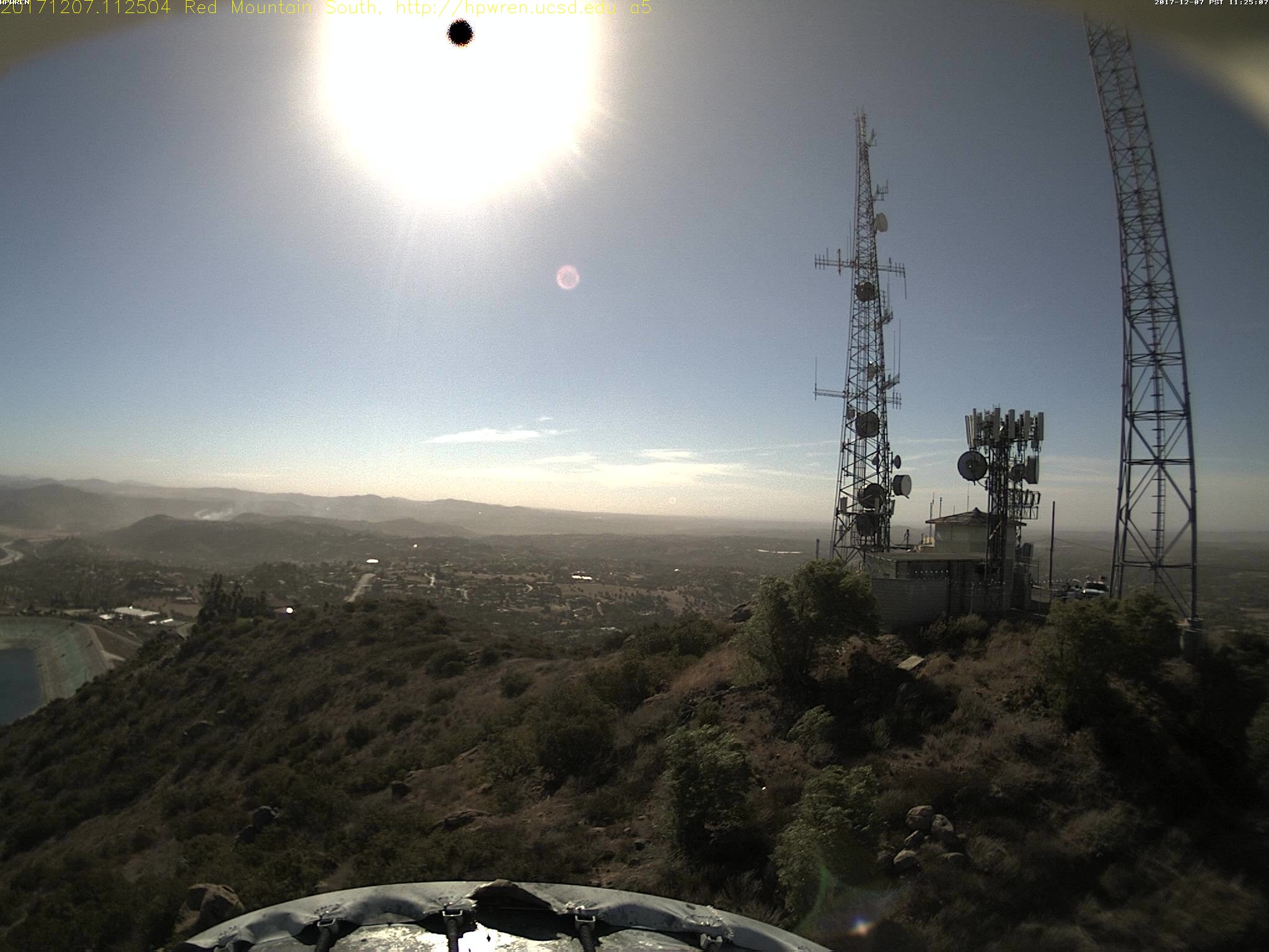
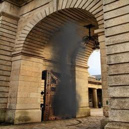
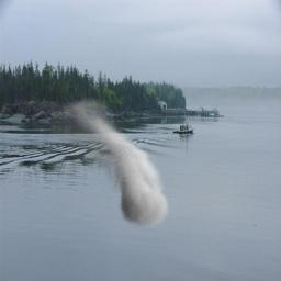
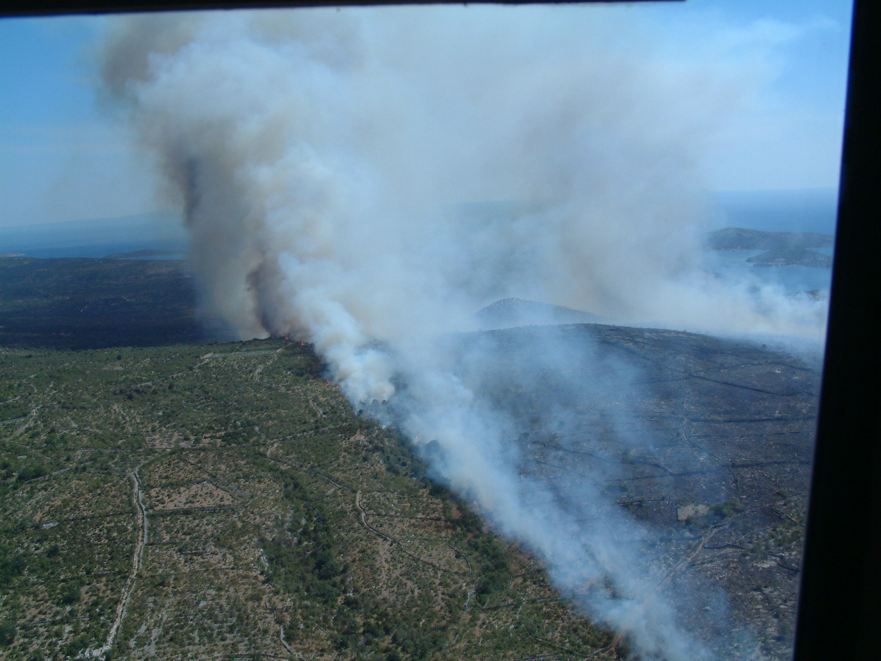
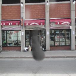
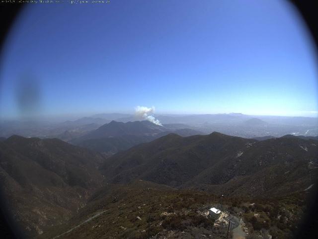
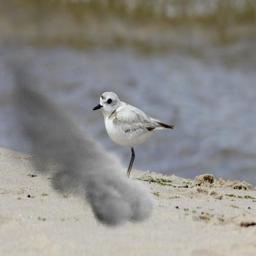
a	b	c	d	e

Figure 7: Comparison between SYN70K and real images in our SMOKE5K dataset. From left to right: (a) the image in SYN70K. (b) the ground truth in SMOKE5K. (c) the image in SMOKE5K. (d) the ground truth in SMOKE5K. (e) the scribble annotation in SMOKE5K.

Also, smoke images are difficult to precisely label due to the challenging attributes mentioned above, thus we also provide scribble annotations for weakly supervised smoke segmentation, shown in Fig.7 (e). Weakly supervised learning allows a model to learn from a weak supervision signal i.e. image-level (Zhou et al. 2015; Wang et al. 2018), scribble-level (Lin et al. 2016a), bounding box-level (Khoreva et al. 2016; Dai, He, and Sun 2015) annotations. Scribble annotation is especially suitable for smoke segmentation as: 1) compared with pixel-wise annotation, scribble annotation is much cheaper and faster (It only takes 2$\sim$5 seconds for each image); 2) compared with image-level annotation, scribble annotation is effective for localizing small objects; 3) compared with bounding box-level annotation, scribble annotation is more flexible for diverse shape objects.

Dataset Visualisation

The qualitative comparisons between SYN70K and our real images are visualized in Fig.7, which further demonstrates the superior of our dataset.

Qualitative Results

Comprehensive qualitative comparisons are visualized in Fig. 8. It can be seen that our model can perform well in smoke with different scales, different shapes, and semi-transparent properties. As shown in Fig.8, our model can capture the structure information well, which shows the effectiveness of our transmission loss.

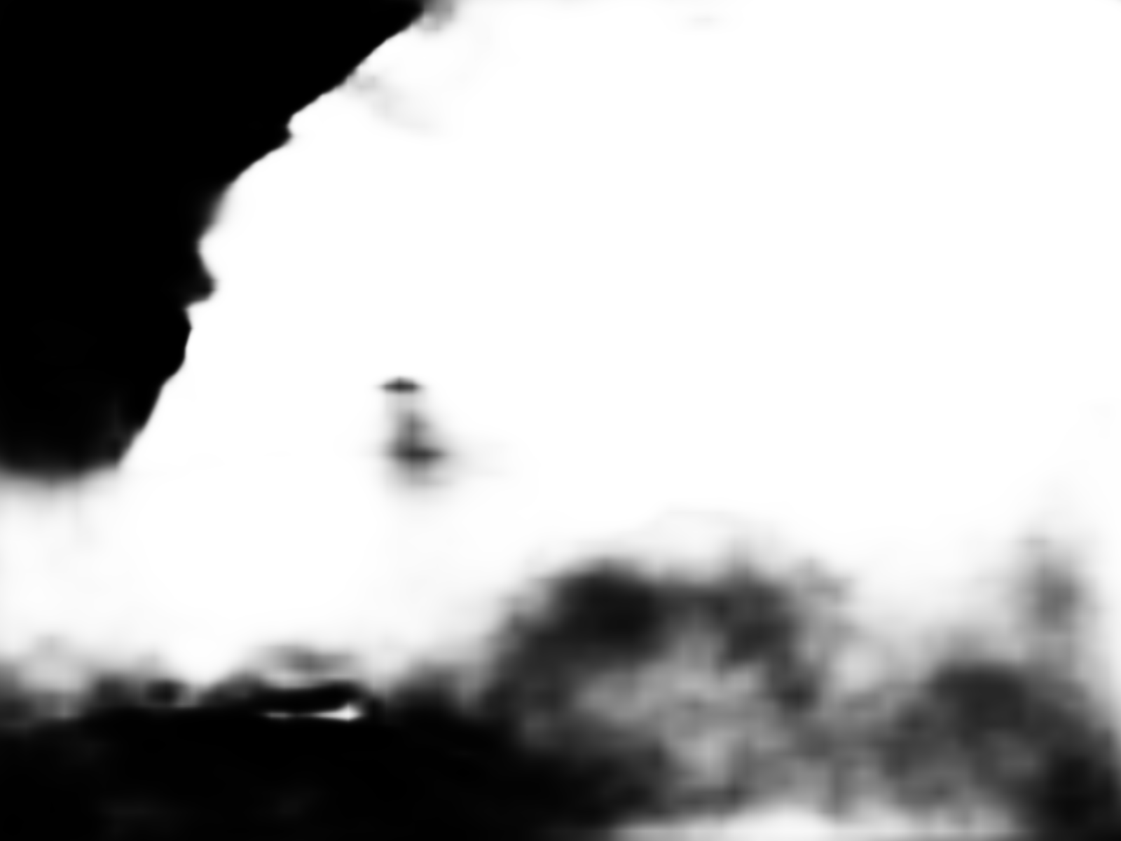
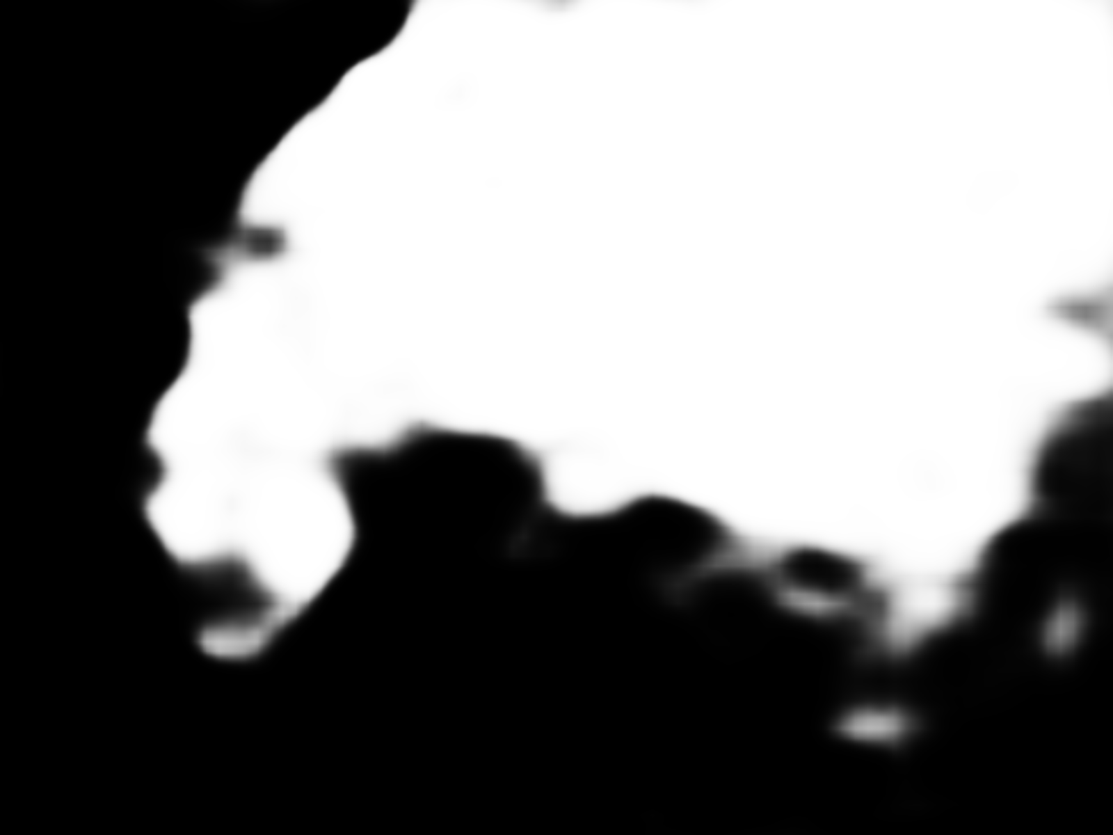
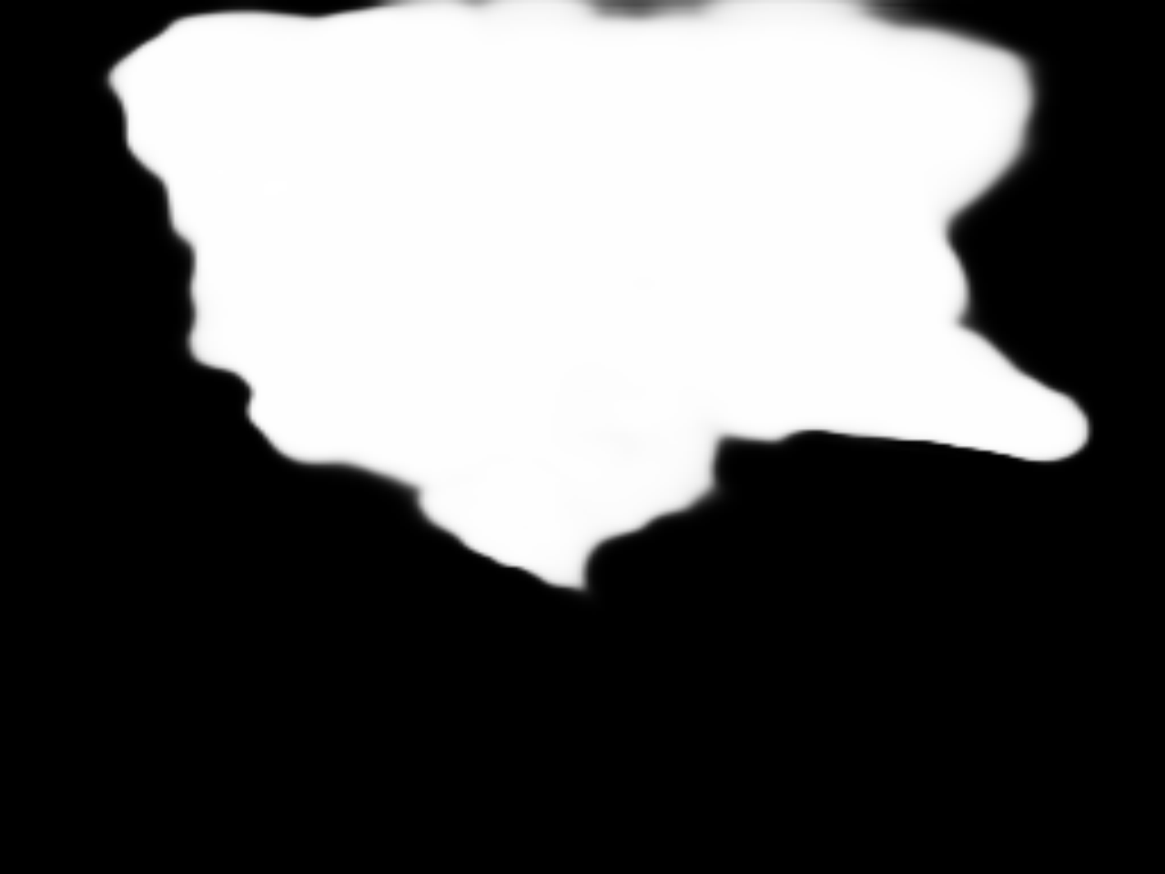
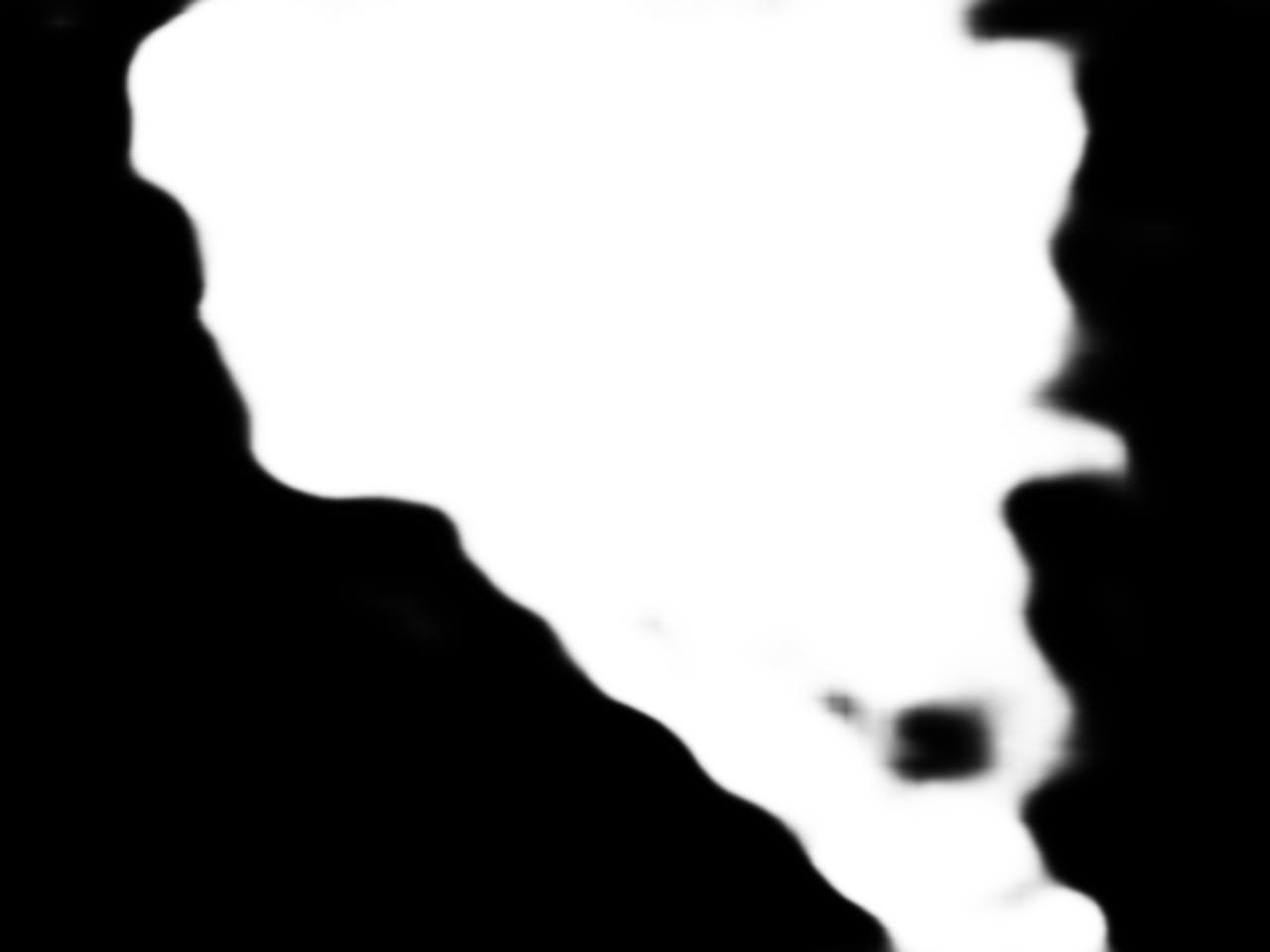
Image	GT	F3Net	BASNet	SCRN	ITSD	UCNet	Our

Figure 8: Qualitative comparison of predictions by our model and other state-of-the-other models. The last two rows are smoke with different location in the same scenes.

Dark Channel Prior Algorithm

In this section, we introduce how we estimate the transmission map using the dark channel algorithm (He, Sun, and Tang 2011) in more detail. It mainly includes two components.

Firstly, the dark channel of images is computed by

$$I^{dark}(m)=\min\limits_{c\in{r,g,b}}(\min\limits_{n\in K(m)}(I^{c}(n)))$$ (15)

where $I^{c}$ is a color channel of an image $I$ and $K(m)$ is a local kernel of size $k\times k$ centered at $m$.

Secondly, we can estimate the transmission information of each pixel of the intensity image by:

$$T(m)=1-\min\limits_{c}(\min\limits_{n\in K(m)}(\frac{I^{c}(n)}{A^{c}}))$$ (16)

where $A$ is global atmospheric light, $I$ is the intensity image, $c$ is the color channel, $K(m)$ is a local patch of size $k\times k$ centered at pixel $m$ and then $\min\limits_{c}(\min\limits_{n\in K(m)}(\frac{I^{c}(n)}{A^{c}})$ is the normalized haze map defiend by (He, Sun, and Tang 2011). We can see the estimated medium transmission is based on the global atmospheric light $A$. To get $A$, we follow (He, Sun, and Tang 2011) and obtain it by picking the top $0.1\%$ brightest pixels in the dark channel $I^{dark}$ of the intensity image. Finally, we use a guided filter (He, Sun, and Tang 2013) to refine transmission map $T$. The whole algorithm is described in Algorithm 1.

Algorithm 1 Dark channel prior based alogrithm.

Input: RGB image $I$.

Output: A transmission map $\hat{T}.$

1:  Calculate the dark channel image based on Equation 15;

2:  Estimate the global atmosphere light $A$ by picking the top 0.1% brightest pixels in the dark channel, and the pixels with the highest intensity in the input image $I$ is selected as the atmospheric light $A$.;

3:  Calculate the transmission map $T$ in Equation 16;

4:  Get the refined transmission map $\hat{T}$ by a guided filter; return $\hat{T}$;

Discussions about Model detail

Hyperparameter Analysis: (1) The dimension of latent space is important for the model’s performance. We tried different numbers in the range: [2-32], and find relatively stable performance in the range: [8-16]. We finally set the latent space dimension as 8, yielding the best performance. (2) For the weights of different losses, empirically, we tried the transmission loss weight $\lambda_{1}$ in the range: [0.1-0.6], and observed the best performance when $\lambda_{1}=0.3$ and the worst when $\lambda_{1}=0.6$. For the uncertainty calibration loss weight $\lambda_{2}$, we tried the range: [0.005-0.1], and observed the best performance when $\lambda_{2}=0.01$.
Inference Time: Processing speed is also an important factor for real-time smoke segmentation. During the inference stage, we only need to keep a portion of the model, which is the Bayesian latent variable model, to produce smoke detection results with no sampling process. Compared with conventional segmentation models, our model only additionally introduces a five layers CNN model. For input images of size 480 x 480, our model can process 6 images/sec, which is comparable with conventional segmentation models.

References

- Babaee, Dinh, and Rigoll (2017) Babaee, M.; Dinh, D. T.; and Rigoll, G. 2017. A Deep Convolutional Neural Network for Background Subtraction. CoRR, abs/1702.01731.
- Baidya (2018) Baidya, A. 2018. Smoke Semantic Segmentation. https://github.com/rekon/Smoke-semantic-segmentation. Accessed: 2021-6-12.
- Blundell et al. (2015) Blundell, C.; Cornebise, J.; Kavukcuoglu, K.; and Wierstra, D. 2015. Weight Uncertainty in Neural Networks. ArXiv, abs/1505.05424.
- Chang et al. (2020) Chang, J.; Lan, Z.; Cheng, C.; and Wei, Y. 2020. Data Uncertainty Learning in Face Recognition. IEEE Conference on Computer Vision and Pattern Recognition (CVPR), 5709–5718.
- Chen et al. (2018) Chen, L.-C.; Papandreou, G.; Kokkinos, I.; Murphy, K.; and Yuille, A. L. 2018. DeepLab: Semantic Image Segmentation with Deep Convolutional Nets, Atrous Convolution, and Fully Connected CRFs. IEEE Transactions on Pattern Analysis and Machine Intelligence (TPAMI), 40(4): 834–848.
- Dai, He, and Sun (2015) Dai, J.; He, K.; and Sun, J. 2015. BoxSup: Exploiting Bounding Boxes to Supervise Convolutional Networks for Semantic Segmentation. CoRR, abs/1503.01640.
- Depeweg et al. (2018) Depeweg, S.; Hernández-Lobato, J. M.; Doshi-Velez, F.; and Udluft, S. 2018. Decomposition of Uncertainty in Bayesian Deep Learning for Efficient and Risk-sensitive Learning. In International Conference on Machine Learning (ICML).
- Der Kiureghian and Ditlevsen (2009) Der Kiureghian, A.; and Ditlevsen, O. 2009. Aleatory or Epistemic? Does It Matter? Structural Safety, 31: 105–112.
- Ding et al. (2018) Ding, H.; Jiang, X.; Shuai, B.; Liu, A. Q.; and Wang, G. 2018. Context Contrasted Feature and Gated Multi-scale Aggregation for Scene Segmentation. In IEEE Conference on Computer Vision and Pattern Recognition (CVPR), 2393–2402.
- Donida Labati et al. (2013) Donida Labati, R.; Genovese, A.; Piuri, V.; and Scotti, F. 2013. Wildfire Smoke Detection Using Computational Intelligence Techniques Enhanced With Synthetic Smoke Plume Generation. IEEE Trans. on Systems, Man, and Cybernetics: Systems, 43(4): 1003–1012.
- Duvenaud, Maclaurin, and Adams (2016) Duvenaud, D.; Maclaurin, D.; and Adams, R. P. 2016. Early Stopping as Nonparametric Variational Inference. ArXiv, abs/1504.01344.
- Fu et al. (2018) Fu, J.; Liu, J.; Tian, H.; Fang, Z.; and Lu, H. 2018. Dual Attention Network for Scene Segmentation. CoRR, abs/1809.02983.
- Gal and Ghahramani (2016) Gal, Y.; and Ghahramani, Z. 2016. Dropout as a Bayesian Approximation: Representing Model Uncertainty in Deep Learning. ArXiv, abs/1506.02142.
- Guo et al. (2017) Guo, C.; Pleiss, G.; Sun, Y.; and Weinberger, K. Q. 2017. On Calibration of Modern Neural Networks. In International Conference on Machine Learning (ICML), 1321–1330. JMLR.org.
- He et al. (2021) He, H.; Li, X.; Cheng, G.; Shi, J.; Tong, Y.; Meng, G.; Prinet, V.; and Weng, L. 2021. Enhanced Boundary Learning for Glass-like Object Segmentation. arXiv:2103.15734.
- He, Sun, and Tang (2011) He, K.; Sun, J.; and Tang, X. 2011. Single Image Haze Removal Using Dark Channel Prior. IEEE Transactions on Pattern Analysis and Machine Intelligence (TPAMI), 33(12): 2341–2353.
- He, Sun, and Tang (2013) He, K.; Sun, J.; and Tang, X. 2013. Guided Image Filtering. IEEE Transactions on Pattern Analysis and Machine Intelligence, 35(6): 1397–1409.
- He et al. (2015) He, K.; Zhang, X.; Ren, S.; and Sun, J. 2015. Deep Residual Learning for Image Recognition. CoRR, abs/1512.03385.
- Hu, Sclaroff, and Saenko (2020) Hu, P.; Sclaroff, S.; and Saenko, K. 2020. Uncertainty-Aware Learning for Zero-Shot Semantic Segmentation. In Conference on Neural Information Processing Systems (NeurIPS).
- Hu et al. (2019) Hu, S.; Worrall, D.; Knegt, S.; Veeling, B.; Huisman, H.; and Welling, M. 2019. Supervised Uncertainty Quantification for Segmentation with Multiple Annotations. arXiv:1907.01949.
- Islam et al. (2017) Islam, M. A.; Naha, S.; Rochan, M.; Bruce, N. D. B.; and Wang, Y. 2017. Label Refinement Network for Coarse-to-Fine Semantic Segmentation. CoRR, abs/1703.00551.
- Jiawei Liu (2022) Jiawei Liu, N. B., Jing Zhang. 2022. Modeling Aleatoric Uncertainty for Camouflaged Object Detection. In IEEE Winter Conference on Applications of Computer Vision (WACV).
- Kendall and Gal (2017) Kendall, A.; and Gal, Y. 2017. What Uncertainties Do We Need in Bayesian Deep Learning for Computer Vision? CoRR, abs/1703.04977.
- Khoreva et al. (2016) Khoreva, A.; Benenson, R.; Hosang, J. H.; Hein, M.; and Schiele, B. 2016. Weakly Supervised Semantic Labelling and Instance Segmentation. CoRR, abs/1603.07485.
- Kohl et al. (2018) Kohl, S. A. A.; Romera-Paredes, B.; Meyer, C.; Fauw, J.; Ledsam, J.; Maier-Hein, K.; Eslami, S.; Rezende, D. J.; and Ronneberger, O. 2018. A Probabilistic U-Net for Segmentation of Ambiguous Images. In Conference on Neural Information Processing Systems (NeurIPS).
- Lakshminarayanan, Pritzel, and Blundell (2017) Lakshminarayanan, B.; Pritzel, A.; and Blundell, C. 2017. Simple and Scalable Predictive Uncertainty Estimation using Deep Ensembles. In Conference on Neural Information Processing Systems (NeurIPS).
- Li et al. (2021a) Li, A.; Zhang, J.; Lyu, Y.; Liu, B.; Zhang, T.; and Dai, Y. 2021a. Uncertainty-aware Joint Salient Object and Camouflaged Object Detection. In IEEE Conference on Computer Vision and Pattern Recognition (CVPR).
- Li et al. (2021b) Li, C.; Anwar, S.; Hou, J.; Cong, R.; Guo, C.; and Ren, W. 2021b. Underwater Image Enhancement via Medium Transmission-Guided Multi-Color Space Embedding. CoRR, abs/2104.13015.
- Li et al. (2016) Li, C.; Guo, J.; Cong, R.; Pang, Y.; and Wang, B. 2016. Underwater Image Enhancement by Dehazing With Minimum Information Loss and Histogram Distribution Prior. IEEE Transactions on Image Processing (TIP), 25: 5664–5677.
- Li et al. (2020) Li, X.; Chen, Z.; Wu, Q. M. J.; and Liu, C. 2020. 3D Parallel Fully Convolutional Networks for Real-Time Video Wildfire Smoke Detection. IEEE Trans. on Circuits and Systems for Video Technology, 30(1): 89–103.
- Lin et al. (2016a) Lin, D.; Dai, J.; Jia, J.; He, K.; and Sun, J. 2016a. ScribbleSup: Scribble-Supervised Convolutional Networks for Semantic Segmentation. CoRR, abs/1604.05144.
- Lin et al. (2016b) Lin, G.; Milan, A.; Shen, C.; and Reid, I. D. 2016b. RefineNet: Multi-Path Refinement Networks for High-Resolution Semantic Segmentation. CoRR, abs/1611.06612.
- Long, Shelhamer, and Darrell (2014) Long, J.; Shelhamer, E.; and Darrell, T. 2014. Fully Convolutional Networks for Semantic Segmentation. CoRR, abs/1411.4038.
- Miao, Chen, and Wang (2014) Miao, L.; Chen, Y.; and Wang, A. 2014. Video smoke detection algorithm using dark channel priori. In CCC 2014.
- Neal (1996) Neal, R. M. 1996. Bayesian Learning for Neural Networks. Berlin, Heidelberg: Springer-Verlag. ISBN 0387947248.
- Newell, Yang, and Deng (2016) Newell, A.; Yang, K.; and Deng, J. 2016. Stacked Hourglass Networks for Human Pose Estimation. CoRR, abs/1603.06937.
- Peng et al. (2017) Peng, C.; Zhang, X.; Yu, G.; Luo, G.; and Sun, J. 2017. Large Kernel Matters - Improve Semantic Segmentation by Global Convolutional Network. CoRR, abs/1703.02719.
- Qin et al. (2019) Qin, X.; Zhang, Z.; Huang, C.; Gao, C.; Dehghan, M.; and Jagersand, M. 2019. BASNet: Boundary-Aware Salient Object Detection. In IEEE Conference on Computer Vision and Pattern Recognition (CVPR), 7479–7489.
- Ronneberger, Fischer, and Brox (2015) Ronneberger, O.; Fischer, P.; and Brox, T. 2015. U-Net: Convolutional Networks for Biomedical Image Segmentation. CoRR, abs/1505.04597.
- Rupprecht et al. (2017) Rupprecht, C.; Laina, I.; DiPietro, R.; and Baust, M. 2017. Learning in an Uncertain World: Representing Ambiguity Through Multiple Hypotheses. IEEE International Conference on Computer Vision (ICCV), 3611–3620.
- Shi, Lu, and Cui (2019a) Shi, X.; Lu, N.; and Cui, Z. 2019a. Smoke Detection Based on Dark Channel and Convolutional Neural Networks. In Int. Conf. on Big Data and Information Analytics, 23–28.
- Shi, Lu, and Cui (2019b) Shi, X.; Lu, N.; and Cui, Z. 2019b. Smoke Detection Based on Dark Channel and Convolutional Neural Networks. Int. Conf. on Big Data and Information Analytics (BigDIA), 23–28.
- Sohn, Lee, and Yan (2015) Sohn, K.; Lee, H.; and Yan, X. 2015. Learning Structured Output Representation using Deep Conditional Generative Models. In Conference on Neural Information Processing Systems (NeurIPS).
- Wang, Shen, and Shao (2018) Wang, W.; Shen, J.; and Shao, L. 2018. Video Salient Object Detection via Fully Convolutional Networks. IEEE Transactions on Image Processing (TIP), 27(1): 38–49.
- Wang et al. (2018) Wang, X.; You, S.; Li, X.; and Ma, H. 2018. Weakly-Supervised Semantic Segmentation by Iteratively Mining Common Object Features. CoRR, abs/1806.04659.
- Wei, Wang, and Huang (2019) Wei, J.; Wang, S.; and Huang, Q. 2019. F3Net: Fusion, Feedback and Focus for Salient Object Detection. CoRR, abs/1911.11445.
- Wu, Su, and Huang (2019) Wu, Z.; Su, L.; and Huang, Q. 2019. Stacked Cross Refinement Network for Edge-Aware Salient Object Detection. In IEEE International Conference on Computer Vision (ICCV).
- Xie et al. (2020) Xie, E.; Wang, W.; Wang, W.; Ding, M.; Shen, C.; and Luo, P. 2020. Segmenting Transparent Objects in the Wild. CoRR, abs/2003.13948.
- Xu et al. (2019) Xu, G.; Zhang, Y.; Zhang, Q.; Lin, G.; Wang, Z.; Jia, Y.; and Wang, J. 2019. Video Smoke Detection Based on Deep Saliency Network. Fire Safety Journal, 105.
- Yang et al. (2018) Yang, M.; Yu, K.; Zhang, C.; Li, Z.; and Yang, K. 2018. DenseASPP for Semantic Segmentation in Street Scenes. In IEEE Conference on Computer Vision and Pattern Recognition (CVPR), 3684–3692.
- Yu et al. (2018) Yu, C.; Wang, J.; Peng, C.; Gao, C.; Yu, G.; and Sang, N. 2018. Learning a Discriminative Feature Network for Semantic Segmentation. CoRR, abs/1804.09337.
- Yuan et al. (2020) Yuan, F.; Zhang, L.; Xia, X.; Huang, Q.; and Li, X. 2020. A Wave-Shaped Deep Neural Network for Smoke Density Estimation. IEEE Transactions on Image Processing (TIP), 29: 2301–2313.
- Yuan et al. (2021) Yuan, F.; Zhang, L.; Xia, X.; Huang, Q.; and Li, X. 2021. A Gated Recurrent Network With Dual Classification Assistance for Smoke Semantic Segmentation. IEEE Transactions on Image Processing (TIP), 30: 4409–4422.
- Yuan et al. (2018) Yuan, F.; Zhang, L.; Xia, X.; Wan, B.; Huang, Q.; and Li, X. 2018. Deep Smoke Segmentation. CoRR, abs/1809.00774.
- Zhang et al. (2020a) Zhang, J.; Dai, Y.; Yu, X.; Harandi, M.; Barnes, N.; and Hartley, R. I. 2020a. Uncertainty-Aware Deep Calibrated Salient Object Detection. CoRR, abs/2012.06020.
- Zhang et al. (2020b) Zhang, J.; Fan, D.-P.; Dai, Y.; Anwar, S.; Sadat Saleh, F.; Zhang, T.; and Barnes, N. 2020b. UC-Net: Uncertainty Inspired RGB-D Saliency Detection via Conditional Variational Autoencoders. In IEEE Conference on Computer Vision and Pattern Recognition (CVPR).
- Zhang et al. (2021a) Zhang, J.; Fan, D.-P.; Dai, Y.; Anwar, S.; Saleh, F.; Aliakbarian, S.; and Barnes, N. 2021a. Uncertainty Inspired RGB-D Saliency Detection. IEEE Transactions on Pattern Analysis and Machine Intelligence (TPAMI).
- Zhang et al. (2021b) Zhang, J.; Fan, D.-P.; Dai, Y.; Yu, X.; Zhong, Y.; Barnes, N.; and Shao, L. 2021b. RGB-D Saliency Detection via Cascaded Mutual Information Minimization. In IEEE International Conference on Computer Vision (ICCV).
- Zhang et al. (2021c) Zhang, J.; Xie, J.; Barnes, N.; and Li, P. 2021c. Learning Generative Vision Transformer with Energy-Based Latent Space for Saliency Prediction. In Conference on Neural Information Processing Systems (NeurIPS).
- Zhang et al. (2021d) Zhang, J.; Zhu, H.; Wang, P.; and Ling, X. 2021d. ATT Squeeze U-Net: A Lightweight Network for Forest Fire Detection and Recognition. IEEE Access, 9: 10858–10870.
- Zhao et al. (2016) Zhao, H.; Shi, J.; Qi, X.; Wang, X.; and Jia, J. 2016. Pyramid Scene Parsing Network. CoRR, abs/1612.01105.
- Zhou et al. (2015) Zhou, B.; Khosla, A.; Lapedriza, À.; Oliva, A.; and Torralba, A. 2015. Learning Deep Features for Discriminative Localization. CoRR, abs/1512.04150.
- Zhou et al. (2020) Zhou, H.; Xie, X.; Lai, J.-H.; Chen, Z.; and Yang, L. 2020. Interactive Two-Stream Decoder for Accurate and Fast Saliency Detection. In IEEE Conference on Computer Vision and Pattern Recognition (CVPR).
- Zhou et al. (2016) Zhou, Z.; Shi, Y.; Gao, Z.; and Li, S. 2016. Wildfire smoke detection based on local extremal region segmentation and surveillance. Fire Safety Journal, 85: 50–58.