Leveraging Redundancy in multiple audio signals
for Far-Field Speech Recognition

Abstract

To achieve robust far-field automatic speech recognition (ASR), existing techniques typically employ an acoustic front end (AFE) cascaded with a neural transducer (NT) ASR model. The AFE output, however, could be unreliable, as the beamforming output in AFE is steered to a wrong direction. A promising way to address this issue is to exploit the microphone signals before the beamforming stage and after the acoustic echo cancellation (post-AEC) in AFE. We argue that both, post-AEC and AFE outputs, are complementary and it is possible to leverage the redundancy between these signals to compensate for potential AFE processing errors. We present two fusion networks to explore this redundancy and aggregate these multi-channel (MC) signals: (1) Frequency-LSTM based, and (2) Convolutional Neural Network based fusion networks. We augment the MC fusion networks to a conformer transducer model and train it in an end-to-end fashion. Our experimental results on commercial virtual assistant tasks demonstrate that using the AFE output and two post-AEC signals with fusion networks offers up to 25.9% word error rate (WER) relative improvement over the model using the AFE output only, at the cost of $\leq$ 2% parameter increase.

Index Terms—  Acoustic front end, AEC, E2E ASR, Conformer Transducer, Convolutional neural network

1 Introduction

Neural transducer (NT) based models, such as the recurrent neural network transducer (RNN-T) [1], the conformer transducer (CT) [2, 3], and the ConvRNN-T [4] have achieved state-of-the-art results in single-channel ASR. In many cases, voice assistants are far from the sound source (such as in smart speakers) and operate in noisy conditions (noise from various sound sources or multiple speakers) which makes the acoustic scenario challenging. For such cases, voice assistants typically employ multi-microphone or microphone-array based acoustic front ends (AFEs) that use beamforming and adaptive noise reduction techniques  [5, 6, 7, 8, 9, 10, 11] to provide an enhanced signal for ASR.

Typically, the AFE is optimized based on a signal-to-noise ratio (SNR) objective under the knowledge of the microphone array geometry and specific noise field assumptions [7]. The resulting enhanced signal could thus be suboptimal for the ASR task, as the optimization does not consider the ASR objective. Moreover, undesired beam switches caused by interfering sources and strong assumptions about the noise field could degrade the performance of the AFE and thus the downstream ASR task. Recently, beamformers [12, 13, 14] built on neural networks have relaxed the above constraints and delivered superior results compared to AFEs based on signal processing methods. Moreover, the neural beamformer can directly be optimized together with the ASR objective in an end-to-end manner [15, 16, 17, 18, 19, 20, 21, 22, 23].

This work is motivated by the opportunity of best exploiting the information generated by an AFE [24], which also includes a multichannel AEC (MCAEC) processing aimed at suppressing playback or other known interference signals. AEC outputs can be complementary to the beamformed signal, in particular under noisy conditions. Thanks to this feature, we design fusion nets that utilize the AFE output and post-AEC signals, and produce a hidden representation that is forwarded to the ASR component, as illustrated in Fig. 1. In this way, the ASR model can be trained in an end-to-end fashion, by exploiting such complementarity. A similar approach was proposed in [25, 26]. However, in [25, 26] all input channels are directly forwarded to the ASR audio encoder, which makes it computationally more expensive and less attractive for streaming ASR.

Two fusion nets are based on (a) the frequency-LSTM [27] with a neural beamformer [15] pre-processing the post-AEC signals (NBF+F-LSTM), and (b) a convolutional neural network (CNN). In the NBF+FLSTM fusion network, we expand the neural beamforming approach of [15] (that was initially proposed for DNN-HMM ASR acoustic modeling) and utilize an F-LSTM to produce the final hidden representation based on the multiple signals. Note that in [15], the authors used pre-AEC microphone signals rather the post-AEC signals. The CNN fusion network, on the other hand, is inspired by [4, 28, 29], but here we use convolutions to model multi-channel signals. Our fusion networks are used to augment a CT ASR model [2, 3]. Note that all of our models are trained end-to-end, are streamable, while the fusion network adds less than $2\%$ of additional parameters in the model architecture. Our experiments show that the proposed methods outperform the CT with only the AFE output, offering up to 25.9% WER relative improvement.

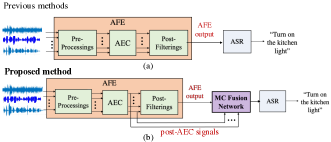
Fig. 1: A high level diagram of the proposed method. Different from previous methods [20, 21, 22, 23, 15] (a), we leverage the redundancy between the AFE output and post-AEC signals via a MC fusion network (b), before feeding the signal to the ASR model.

2 Neural transducers for ASR

A shared component between the baseline system (Fig.1(a)) and our method (Fig.1(b)) is the NT ASR. It typically consists of an encoder network, a prediction network and a joint network. The encoder network encodes the input time frames $\mathbf{x_{t}}$ into high level representations $h_{t}^{enc}$. The prediction network uses the previously predicted word-pieces $\mathbf{y_{u-1}}$ and produces the intermediate representations $h_{u}^{pred}$. The joint network combines the representations of $h_{t}^{enc}$ and $h_{u}^{pred}$ by first applying a joint operation and passing the output through a series of dense layers with activations and a final softmax that gives the probability distribution of word-pieces.The neural transducer is trained based on the RNN-T loss using the forward-backward algorithm [1] that accounts for all possible alignments between the acoustic frames and the word-pieces of the transcription. The architecture of the encoder and prediction network can vary, with typical choices being RNN layers [1], transformer [30] or conformer blocks [2, 3]. In this work, we use a conformer encoder and an LSTM decoder (CT). Note that our fusion networks can be applied with any NT, and not limited to CT.

3 Proposed MC fusion networks

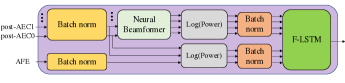
Fig. 2: The neural beamformer+Frequency-LSTM (NBF+F-LSTM) fusion network. Note that the same colored batch norm layers indicates the shared parameters.

Our goal is to empower the CT ASR model to leverage multiple signals processed by different techniques and explore the redundancy, including (1) An enhanced signal produced by a signal processing based AFE [24] that performs MCAEC, adaptive beamforming and noise reduction, and (2) The signals after AEC (post-AEC signals). These signals are processed by the MC fusion network (Figure 1) leading to a high level representation that is input to the encoder network of the CT model. We propose two MC fusion networks.

3.1 Neural beamformer (NBF)+F-LSTM Fusion Network

This approach utilizes a trainable neural beamformer inspired from [15] where authors used neural beamforming techniques for DNN-HMM ASR acoustic modeling. The approach is comprised of two major steps: a neural beamformer to perform spatial filtering on the multichannel inputs and a Frequency LSTM (F-LSTM) [27] layer to combine the AFE output and post-AEC signals. The architecture of the fusion network is shown in Figure 2. First, a batch normalization is applied on the frequency bins of the input signals to stabilize the training and make convergence faster.

Neural beamforming network. The $M$ batch normalized post-AEC signals $\mathbf{X}(t,\omega)$ enter the neural beamforming block, where a filtering operation is performed as:

$$Y(t,\omega,\mathbf{p})=\mathbf{w}^{H}(t,\omega,\mathbf{p})\mathbf{X}(t,\omega)$$ (1)

where $H$ denotes the Hermitian operation, $\mathbf{w}(t,\omega,\mathbf{p})$ is a complex weight vector for beamforming at position $\mathbf{p}$; $t$ and $\omega$ denote the time frame and angular frequency.

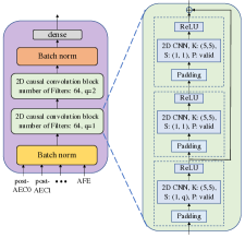
Fig. 3: The Convolutional (CNN) based fusion network

The complex vector multiplication in Eq. (1) for a given frequency $\omega$ can be expressed in matrix form as:

$$\begin{bmatrix}Re(Y)\\ Im(Y)\end{bmatrix}=\begin{bmatrix}Re(w_{0})&Im(w_{0})\\ -Im(w_{0})&Re(w_{0})\\ \vdots&\vdots\\ Re(w_{M-1})&Im(w_{M-1})\\ -Im(w_{M-1})&Re(w_{M-1})\end{bmatrix}^{T}\begin{bmatrix}Re(X_{0})\\ Im(X_{0})\\ \vdots\\ Re(X_{M-1})\\ Im(X_{M-1})\end{bmatrix}$$ (2)

where $(t,\omega,\mathbf{p})$ have been omitted for clarity and $w_{i}$ denotes the i-th element of the complex beamforming weight vector $\mathbf{w}$. Given this formulation, the beamforming operation can be incorporated into the neural network by using $\Omega$ $2\times 2M$ matrices (one for each frequency bin), where $\Omega$ is the total number of frequency bins. These matrices represent the beamformer weights. Note that the complex signal features are treated as two real-valued inputs; both the real and imaginary parts of the complex neural beamformer weights are learnable.

Initially, the weights are initialized to steer the beamformer into $n_{l}$ look directions that are uniformly distributed around the array. During training, the $n_{l}$ sets of weights are optimized according to the RNN-T loss function. The neural beamformer produces $n_{l}$ signals in $n_{l}$ look directions. Next, all neural beamformed signals are considered together with the original microphone array signals and the AFE output. These are a total number of $n_{l}+M+1$ signals. For each signal, we compute its power for each frequency bin, by applying a square and sum operator to the real and imaginary parts. The powers then go through a ReLU activation function and a log function (that also operate on the frequency axis), in order to get an estimate of the log power spectrum. Finally, we add another batch normalization layer operating on the frequency axis of each signal.

Fusion using Frequency LSTMs. Finally, the $n_{l}+M+1$ signals are fused into a single hidden representation. For that, we apply an F-LSTM layer [27]. An F-LSTM is a regular LSTM layer that operates on the frequency axis instead of the time axis. To prepare the input for the F-LSTM, we concatenate all signals together in one vector and take chunks along the frequency axis with a certain window $w$ and stride $s$ in order to create sequences in the frequency domain of length $w$. This input is then passed through an LSTM. The output of the LSTM is projected to a hidden representation of $d_{flstm}$ that is the input to the audio encoder of the CT.

3.2 Convolutional Neural Network (CNN) Fusion Network

Figure 3 illustrates the Convolutional Neural Network (CNN) based MC fusion network. Its design is motivated by ConvRNN-T [4] with several adaptations. First, the input channels contain the AFE output and post-AEC signals. They are concatenated together to form a tensor of $T\times\Omega\times C$, where $T$ is the number of time-frames, $\Omega$ is the number of frequency bins, and $C=M+1$ is the number of input channels. The tensor is mean-normalized by the batch norm layer over the frequency axis before feeding into the two convolutional blocks. The preliminary studies show that this batch norm is critical to stabilize the training. Each convolutional block has three convolutional layers and we use two blocks leading to 6 convolutional layers in total, as shown in Figure 3. Each convolutional layer is followed by a ReLU activation, and an additional residual link is added from the first ReLU input with the output. To ensure the convolution computations are causal (since our model is streamable), we zero-pad the time dimension from the left with kernel size ($K$) minus one zeros. Note that the second convolutional block downsamples the frequency bins by two (stride size $q=2$) to maintain the model size. After the convolutional blocks, the second batch norm normalizes both the mean and scale of CNN outputs along the frequency axis, which we found offering better convergence in our studies. The final dense layer then projects the normalized outputs to the $d_{cnn}$ dimension, and feed it to the CT audio encoder.

4 Experiments

4.1 Datasets

To evaluate the proposed methods, we conduct a series of ASR experiments using our in-house de-identified far-field datasets . The datasets are for the English language and virtual assistant tasks. The device-directed speech data was captured using a smart speaker with 7 microphones, and a 63 mm aperture. The training sets contain $\sim 500K$ hours of single-channel (SC) data and $\sim 60K$ hours of multi-channel (MC) data. The SC data consists of the AFE output [24]; the AFE takes as input the 7 microphone signals. The MC data contains 2 post-AEC signals of aperture distance in addition to the AFE output. When training/testing the MC models on the SC data (which only contains the AFE output), we simply replace the 2 post-AEC signals with zeros.

We use the following SC and MC test sets: (1) Head: 10 hours of SC data that represent the head distribution of a far-field voice assistant task. (2) MC clean: 3 hours of MC data of high SNR for a virtual assistant task. (3) MC noisy: 20 hours of MC data for a virtual assistant task collected in a controlled condition. This dataset contains more challenging acoustic scenarios covering two common device locations and three noise conditions. The Device locations include (1) DevLoc1: The device is right in front of the speaker (5 feet away). (2) DevLoc2: The device is in front of the speaker but far away in the corner (15 feet away). The noise conditions are (1) Silence: no background noise (2) Appliance: appliance noises, e.g., air conditioner, and (3) Media: The noises from the TV, radio, etc.

4.2 Model Configurations

4.2.1 Baseline methods

We use the conformer transducer (CT) as the ASR component for all the following baseline models. (1) AFE CT: It serves as the baseline using only the AFE output and no fusion net. (2) CA CT: This baseline uses the channel attention (CA) based fusion network as proposed in [26]. We feed both AFE output and post-AECs to this model for evaluating our fusion networks. To maintain the comparable model size, we employ one cross-channel attention layer and select the best number of attention heads (among 1, 2, 4) and head sizes (among 512, 256, 128) based on the validation set performances. All CTs in the baselines share the same configurations: Two convolutional layers followed by 14 conformer blocks. The convolutional layers have 128 kernels of size 3, the stride of 2 and 1 along the time axis for the first and second convolution respectively. Each conformer block contains the FeedForwardNetwork (FFN) module with 1024 units, the convolutional module with kernel size 15, and the attention module with the embedding size 512, and 8 heads. The number of parameters is 81.44 million. The CT encoder outputs are projected to 512-dimensional hidden representations, before being fed into the joint network. The prediction network consists of two LSTM layers with 1024 units. The output is also projected to a 512-dimension to match the audio encoder output. The joint network consists of a FFN with 512 units. We used the Adam optimizer [31] and varied the learning rate following [32, 30].

4.2.2 Fusion Networks

Neural beamformer (NBF) + F-LSTM: For the neural beamformer, we set the number of look directions to $n_{l}=4$. Our preliminary analysis showed that increasing look directions does not lead to noticeable improvements. For the F-LSTM layer we use a window of 48 frequency bins with a stride of 15 and employ two bi-directional LSTMs with 16 units. The outputs of the F-LSTM is projected to $d_{flstm}=192$-dimensional vector in match the feature size of baselines. The total number of parameters is 372K, which takes only $\sim 0.5\%$ of the parameter size of the conformer encoder.

Convolutional Fusion Network (CNN): It contains two 2D causal convolution blocks, each of which has three convolutional layers. The first 2D causal convolution block has 64 kernels of size $K$=(5,5), the stride size equals to 1 along both the time axis and the stride size along frequency axis, $q$=1. The second 2D causal convolutional block has the same configuration as the first one but with the stride size along the frequency axis, $q$=2. The final dense layer projects the normalized CNN block outputs to the $d_{cnn}=192$-dimensional vector. The total number of parameters is 1.4M, which takes only $\sim 1.8\%$ of the parameter size of the conformer encoder. All the models are of comparable size, $\sim 82$ million parameters in total.

4.3 Input and Output Configurations

The input features for AFE CT model are Log-filter bank energies (LFBEs) and are extracted with a frame rate of 10 ms with a window size of 32 ms from audio samples sampled at $16$ kHz. The features of each frame are stacked with the ones of left two frames, followed by the downsampling by a factor of 3 to achieve low frame rate, resulting in 192 feature dimensions. The proposed methods use the Short Time Fourier Transform (STFT) features, which are computed with a 512-point Fourier Transform on segments using a 32 ms window with a frame rate of 10 ms. We separate the complex values into their real and imaginary parts, resulting in 512-dimensional features for every frame. Similarly, we use a left context of 3 frames. A subword tokenizer [33] is used to create output tokens from the transcriptions; we use 4K tokens.

5 Results and Discussions

Table 1: WERRs(%) of the proposed models and channel attention (CA) based fusion networks over AFE CT, on the HEAD, MC clean, and MC noisy test sets. All three models use the AFE output and post-AECs as inputs. A higher number indicates a better WER.

. $\text{Fusion Network}(\downarrow)/\text{Testset}(\rightarrow)$ HEAD MC Clean MC Noisy NBF+F-LSTM 5.66 5.31 10.75 CNN 7.76 6.10 10.38 CA [26] 4.61 3.74 8.96

Table 2: Ablation study given WERRs(%) over AFE CT: Comparisons of the proposed models to the ones removing either the fusion network or post-AECs, on the HEAD, MC clean, and MC noisy test sets. A higher number indicates a better WER.

. $\text{Model}(\downarrow)/\text{Testset}(\rightarrow)$ HEAD MC Clean MC Noisy AFE CT baseline baseline baseline + post-AECs+NBF+FLSTM (Ours) 5.66 5.31 10.75 + post-AECs (no fusion net) 1.89 3.54 7.92 + NBF+FLSTM (no post-AECs) 0.84 1.18 6.70 + post-AECs+NBF+CNN (Ours) 7.76 6.10 10.38 + post-AECs (no fusion net) 1.89 3.54 7.92 + CNN (no post-AECs) 5.24 8.66 6.89

We report the relative word error rate reduction (WERR) of the proposed methods against baselines throughout the experiments. Given a model A’s WER ($\text{WER}_{A}$) and a baseline B’s WER ($\text{WER}_{B}$), the WERR of A over B can be computed by $(\text{WER}_{B}-\text{WER}_{A})/\text{WER}_{B}$; a higher WERR value indicates a better performance.

Table 1 presents the WERRs for the proposed models and the baselines on three test sets. By leveraging the post-AEC signals along with the AFE ouput, all the fusion network based CT models perform better than using AFE only (positive WERR values). Besides, the proposed NBF+F-LSTM and CNN fusion networks perform better than the channel-attention based fusion network, which implies better time vs. frequency relationship learning across channels given the comparable model size (Section 4.2.2). We can also see that the improvements from post-AECs and fusion network are more significant on MC Noisy test sets than on MC Clean test set. For example, the WERRs for NBF+FLSTM over AFE CT on MC Noisy is $10.75\%$ versus $5.31\%$ on MC Clean. It implies that the proposed methods are robust to challenging acoustic conditions.

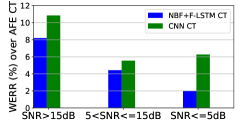
Fig. 4: WERRs(%) of the proposed methods over AFE CT w.r.t. different SNRs. A higher number indicates a better WER.

Impact of fusion networks and post AECs: We evaluate the contribution of each sub-component in our models by removing either fusion networks (no fusion net) or post-AECs (no post-AECs). Note that no fusion net simply concatenates the AFE output and post-AECs and projects to the $d_{flstm}$/$d_{cnn}$=192-dim with a FFN layer. The results are illustrated in Table 2. For NBF+F-LSTM fusion based model, we see that removing post-AECs leads to much smaller WER improvements than removing the fusion network. In the CNN fusion based model, we see the similar trends on HEAD and MC Noisy. Adding post-AECs does not lead to further improvement (6.10% vs. 8.66% from AFE+CNN CT) on MC Clean in this case.
Robustness to different SNRs: In Fig. 4, we further evaluate the model robustness w.r.t. different SNR levels on the HEAD test set. It can be observed that both proposed methods offer improvements across the entire range of SNRs. In accordance to Table 1, the CNN fusion network offers the best improvements.
Robustness to device locations and noise types: Finally, we evaluate our models under different combinations of device locations and noise types provided in MC Noisy test set. The results are presented in Table 3. We see that the proposed models outperform the baselines with no post-AECs under DevLoc2, from $10.52\%$ (NBF+FLSTM CT under Silence noise) to $25.91\%$ (CNN CT under Appliance noise) relative WER improvement. This shows post-AECs benefits AFE for the far-field ASR. Under DevLoc1, we observe smaller improvements with Silence noise as well as Appliance noise, yet $2.28\%$ and $6.71\%$ relative degradations under Media noise. We speculate that in DevLoc1 the noise source is much closer to the target speaker than in DevLoc2. The post-AECs are highly contaminated by Media noise, as a result, do not provide useful complementary information to recover the errors produced by the AFE. In this case, including post-AECs could be detrimental.

Table 3: WERRs (%) of the proposed methods over AFE CT w.r.t. different device locations and noise types. A higher number indicates a better WER.

Device Location	Noise Type	NBF+F-LSTM CT	CNN CT
DevLoc1	Silence	8.23	12.05
$\sim 5$ feet away	Appliance	8.21	6.87
in front of the speaker	Media	-2.28	-6.71
DevLoc2	Silence	10.52	13.86
$\sim 15$ feet away	Appliance	21.47	25.91
in front of the speaker	Media	12.76	17.92

6 Conclusion

We proposed two fusion networks based on NBF+F-LSTM and CNN in order to exploit the redundancy and aggregate the AFE output and post-AEC signals. The experimental results show that our fusion networks are better than the channel attention based fusion network given less than 2% model parameter increase. In addition, our ablation studies demonstrate that exploiting both AFE and post-AEC mic array signals leads to the best improvement, e.g. 10.75% in MC Noisy test set. Moreover, our methods are more robust to different SNRs, device locations, and noise types, achieving up to 25.91% WER relative improvement over AFE CT.

References

- [1] Alex Graves, “Sequence transduction with recurrent neural networks,” ICML workshop, 2012.
- [2] Bo Li, Anmol Gulati, Jiahui Yu, Tara N Sainath, Chung-Cheng Chiu, Arun Narayanan, Shuo-Yiin Chang, Ruoming Pang, Yanzhang He, James Qin, et al., “A better and faster end-to-end model for streaming ASR,” in ICASSP, 2021.
- [3] Anmol Gulati, James Qin, Chung-Cheng Chiu, Niki Parmar, Yu Zhang, Jiahui Yu, Wei Han, Shibo Wang, Zhengdong Zhang, Yonghui Wu, et al., “Conformer: Convolution-augmented transformer for speech recognition,” arXiv preprint arXiv:2005.08100, 2020.
- [4] Martin Radfar, Rohit Barnwal, Rupak Vignesh Swaminathan, Feng-Ju Chang, Grant P Strimel, Nathan Susanj, and Athanasios Mouchtaris, “Convrnn-t: Convolutional augmented recurrent neural network transducers for streaming speech recognition,” Interspeech, 2022.
- [5] Reinhold Haeb-Umbach, Shinji Watanabe, Tomohiro Nakatani, Michiel Bacchiani, Bjorn Hoffmeister, Michael L Seltzer, Heiga Zen, and Mehrez Souden, “Speech processing for digital home assistants: Combining signal processing with deep-learning techniques,” IEEE Signal processing magazine, vol. 36, no. 6, pp. 111–124, 2019.
- [6] Maurizio Omologo, Marco Matassoni, and Piergiorgio Svaizer, “Speech recognition with microphone arrays,” in Microphone arrays, pp. 331–353. Springer, 2001.
- [7] Matthias Wölfel and John McDonough, Distant speech recognition, John Wiley & Sons, 2009.
- [8] Kenichi Kumatani, John McDonough, and Bhiksha Raj, “Microphone array processing for distant speech recognition: From close-talking microphones to far-field sensors,” IEEE Signal Processing Magazine, vol. 29, no. 6, pp. 127–140, 2012.
- [9] Keisuke Kinoshita et al., “A summary of the REVERB challenge: state-of-the-art and remaining challenges in reverberant speech processing research,” EURASIP Journal on Advances in Signal Processing, vol. 2016, no. 1, pp. 7, 2016.
- [10] Tobias Menne, Jahn Heymann, Anastasios Alexandridis, Kazuki Irie, Albert Zeyer, Markus Kitza, Pavel Golik, Ilia Kulikov, Lukas Drude, Ralf Schlüter, Hermann Ney, Reinhold Haeb-Umbach, and Athanasios Mouchtaris, “The RWTH/UPB/FORTH system combination for the 4th chime challenge evaluation,” in CHiME-4 workshop, 2016.
- [11] Reinhold Haeb-Umbach, Jahn Heymann, Lukas Drude, Shinji Watanabe, Marc Delcroix, and Tomohiro Nakatani, “Far-field automatic speech recognition,” Proceedings of the IEEE, vol. 109, no. 2, pp. 124–148, 2020.
- [12] Tsubasa Ochiai, Marc Delcroix, Tomohiro Nakatani, and Shoko Araki, “Mask-based neural beamforming for moving speakers with self-attention-based tracking,” arXiv preprint arXiv:2205.03568, 2022.
- [13] Jahn Heymann, Lukas Drude, and Reinhold Haeb-Umbach, “Neural network based spectral mask estimation for acoustic beamforming,” in ICASSP, 2016.
- [14] Hakan Erdogan and John R et al. Hershey, “Improved mvdr beamforming using single-channel mask prediction networks.,” in Interspeech, 2016.
- [15] Minhua Wu, Kenichi Kumatani, Shiva Sundaram, Nikko Ström, and Björn Hoffmeister, “Frequency domain multi-channel acoustic modeling for distant speech recognition,” in ICASSP, 2019, pp. 6640–6644.
- [16] Tsubasa Ochiai and Shinji Watanabe et al., “Multichannel end-to-end speech recognition,” arXiv preprint arXiv:1703.04783, 2017.
- [17] Xuankai Chang, Wangyou Zhang, Yanmin Qian, Jonathan Le Roux, and Shinji Watanabe, “MIMO-speech: End-to-end multi-channel multi-speaker speech recognition,” in ASRU, 2019.
- [18] Xuankai Chang, Wangyou Zhang, Yanmin Qian, Jonathan Le Roux, and Shinji Watanabe, “End-to-end multi-speaker speech recognition with transformer,” in ICASSP, 2020.
- [19] Kenichi Kumatani, Minhua Wu, Shiva Sundaram, Nikko Ström, and Björn Hoffmeister, “Multi-geometry spatial acoustic modeling for distant speech recognition,” in ICASSP, 2019.
- [20] Bo Li and Tara N Sainath et al., “Neural network adaptive beamforming for robust multichannel speech recognition,” in Interspeech, 2016.
- [21] Xiong Xiao and Shinji Watanabe et al., “Deep beamforming networks for multi-channel speech recognition,” in ICASSP, 2016.
- [22] Zhong Meng and Shinji Watanabe et al., “Deep long short-term memory adaptive beamforming networks for multichannel robust speech recognition,” in ICASSP, 2017.
- [23] Yulan Liu, Pengyuan Zhang, and Thomas Hain, “Using neural network front-ends on far field multiple microphones based speech recognition,” in ICASSP, 2014.
- [24] Robert Ayrapetian, Philip Hilmes, Mohamed Mansour, Trausti Kristjansson, and Carlo Murgia, “Asynchronous acoustic echo cancellation over wireless channels,” in ICASSP, 2021.
- [25] Feng-Ju Chang, Martin Radfar, Athanasios Mouchtaris, Brian King, and Siegfried Kunzmann, “End-to-end multi-channel transformer for speech recognition,” in ICASSP, 2021.
- [26] Feng-Ju Chang, Martin Radfar, Athanasios Mouchtaris, and Maurizio Omologo, “Multi-channel transformer transducer for speech recognition,” Interspeech, 2021.
- [27] Maarten Van Segbroeck, Harish Mallidih, Brian King, I-Fan Chen, Gurpreet Chadha, and Roland Maas, “Multi-view frequency LSTM: An efficient frontend for automatic speech recognition,” 2020.
- [28] Ching-Feng Yeh, Jay Mahadeokar, Kaustubh Kalgaonkar, Yongqiang Wang, Duc Le, Mahaveer Jain, Kjell Schubert, Christian Fuegen, and Michael L Seltzer, “Transformer-transducer: End-to-end speech recognition with self-attention,” arXiv preprint arXiv:1910.12977, 2019.
- [29] Abdelrahman Mohamed, Dmytro Okhonko, and Luke Zettlemoyer, “Transformers with convolutional context for ASR,” arXiv preprint arXiv:1904.11660, 2019.
- [30] Linhao Dong, Shuang Xu, and Bo Xu, “Speech-transformer: a no-recurrence sequence-to-sequence model for speech recognition,” in ICASSP, 2018.
- [31] Diederik P Kingma and Jimmy Ba, “Adam: A method for stochastic optimization,” arXiv preprint arXiv:1412.6980, 2014.
- [32] Ashish Vaswani, Noam Shazeer, Niki Parmar, Jakob Uszkoreit, Llion Jones, Aidan N Gomez, Lukasz Kaiser, and Illia Polosukhin, “Attention is all you need,” in NeurNIPS, 2017.
- [33] Rico Sennrich, Barry Haddow, and Alexandra Birch, “Neural machine translation of rare words with subword units,” in ACL, 2016.