On the Importance of Feature Representation for Flood Mapping using Classical Machine Learning Approaches

Abstract

Climate change has increased the severity and frequency of weather disasters all around the world so that efforts to aid disaster management activities and recovery operations are of high value. Flood inundation mapping based on earth observation data can help in this context, by providing cheap and accurate maps depicting the area affected by a flood event to emergency-relief units in near-real-time. Modern deep neural network architectures require vast amounts of labeled data for training and whilst a large amount of unlabeled data is available, accurately labeling this data is a time-consuming and expensive task. Building upon the recent development of the Sen1Floods11 dataset, which provides a limited amount of hand-labeled high-quality training data, this paper evaluates the potential of five traditional machine learning approaches such as gradient boosted decision trees, support vector machines or quadratic discriminant analysis for leveraging this data source.

By performing a grid-search-based hyperparameter optimization on 23 feature spaces we can show that all considered classifiers are capable of outperforming the current state-of-the-art neural network-based approaches in terms of total IoU on their best-performing feature spaces, despite our approaches being trained only on the small amount of hand labeled optical and SAR data available in this dataset for performing pixel-wise flood inundation mapping. We show that with total and mean IoU values of $0.8751$ and $0.7031$ compared to $0.70$ and $0.5873$ as the previous best-reported results, a simple gradient boosting classifier can significantly improve over the current state-of-the-art neural network based approaches on the Sen1Floods11 test set.

Furthermore, an analysis of the regional distribution of the Sen1Floods11 dataset reveals a problem of spatial imbalance. We show that traditional machine learning models can learn this bias and argue that modified metric evaluations are required to counter artifacts due to spatial imbalance. Lastly, a qualitative analysis shows that this pixel-wise classifier provides highly-precise surface water classifications indicating that a good choice of a feature space and pixel-wise classification can generate high-quality flood maps using optical and SAR data. To facilitate future use of the created feature spaces and the gradient boosting model, we make our code publicly available at: https://github.com/DFKI-Earth-And-Space-Applications/Flood_Mapping_Feature_Space_Importance

[tuk]organization=Department of Computer Science, University of Kaiserslautern-Landau,postcode=67663, city=Kaiserslautern, country=Germany

[dfki]organization=German Research Center for Artificial Intelligence (DFKI),postcode=67663, city=Kaiserslautern, country=Germany

[yamanashi]organization=Department of Civil and Environmental Engineering, University of Yamanashi,postcode=4008511, city=Kofu, country=Japan

1 Introduction

Flood Events are the most frequent and destructive weather disasters (Disaster (CRED)), which have caused severe human and economic losses over the last years (Huang and Jin (2020); Landuyt et al. (2020)), thus causing poverty and destroying lives. Furthermore, due to climate change, these effects will likely get worse in the next years (Wing et al. (2018)). Recently, flood events in central Europe in the Summer of 2021 have caused severe damage in France, Luxembourg, Belgium, Netherlands, Austria, and Germany (Huth and Staut (2021); SWR (2021); Ralf Lachmann (2021); dpa,epa (2021)) and resulted in at least 134 deaths in the Ahrtal, Germany (SWR (2021)).

In these situations, quick emergency relief operations are required to aid the local population in need. Flood inundation maps depict the extend of the flood event in a local area. Therefore, accurate and fast to acquire flood maps, are essential to coordinate rescue efforts and are thus of high practical value. In particular, deep learning based flood mapping utilizing satellite imagery is already in use in the Philippines (de la Cruz et al. (2020)).

Another application of flood mapping consists of providing information for the development and calibration of hydraulic flood forecasting models (Grimaldi et al. (2016)). Whilst these models have shown potential for risk assessment (Wing et al. (2018)) and many solutions have been proposed for simulating flood extend (Merwade et al. (2017); Yamazaki et al. (2011); Li et al. (2016)), verification of these models remains challenging as the number of global gauge stations keeps decreasing (Grimaldi et al. (2016)). In this context, flood mapping can not only help by mitigating the effects of flood events but also by supporting the forecasting of flood effects.

As a data source for flood mapping, remote sensing for earth-observation has shown promising results (Shen et al. (2019); Tsyganskaya et al. (2018); Grimaldi et al. (2016)). Remote sensing hereby refers to the process of measuring physical characteristics of an area at a distance (U.S. Department of the Interior (2022b)), which for the purpose of flood mapping consists of observing the earth-surface using sensors on aerial vehicles or on satellites.

In the context of flood mapping, aerial imagery is typically considered the most reliable source of flood extend data, however, the requirement to perform additional flights for data acquisition may make this impractical, especially in developing countries (Grimaldi et al. (2016)). In contrast, satellite data is available at high velocity and volume in the form of continuous global coverage of the earth-surface. For example, free of charge world-wide satellite data is provided by the European Space Agency’s Copernicus Program (ESA (2022)). Furthermore, different sensors such as Synthetic Aperture Radar (ESA (2022)) or multispectral instruments (ESA (2022b)) are available in varying resolutions (PlanetScope (2022); ESA (2022b); U.S. Department of the Interior (2022a)) thereby providing a large variety of data.

The availability of these three of the four V’s of big data (volume, variety, velocity, veracity) (Díaz (2020)), missing only veracity, results in a need for highly-scalable and cheap solutions requiring no-human interaction. Artificial Intelligence has been shown to provide solutions to these goals in many different application scenarios (Russakovsky et al. (2015); Everingham et al. (2014); Lin et al. (2014)), exceeding human performance (Yu et al. (2022)).

Traditionally, these approaches are based on thresholding algorithms, region growing or multi-temporal change detection (Shen et al. (2019)), however more recently Machine Learning approaches such as Random Forests, Support Vector Machines or Deep Learning are also entering the scene (Tsyganskaya et al. (2018); de la Cruz et al. (2020); Konapala et al. (2021); Bentivoglio et al. (2021); Bai et al. (2021)).

Whilst historical flood databases exist, for example provided by the Dartmouth Flood Observatory (University of Colorado (2022)), these are based on low-quality automatic labels (Grimaldi et al. (2016)) and machine learning ready datasets were missing up until recently (Bonafilia et al. (2020); Rambour et al. (2020); Mateo-Garcia et al. (2021); Drakonakis et al. (2022)).

This has resulted in many studies operating on data that was specifically acquired for the individual paper (Tsyganskaya et al. (2018); Bentivoglio et al. (2021)), furthermore, due to the time and effort required for manually creating flood segmentation maps, accurate ground truth data is rare. Some studies try to avoid this time effort by both training their models and computing their evaluation metrics with respect to automatically generated labels (de la Cruz et al. (2020); Huang and Jin (2020)).

In 2020, Bonafilia et al. proposed the Sen1Floods11 dataset, which contains a limited amount of high-quality hand-labeled data, in combination with a larger weakly labeled dataset (Bonafilia et al. (2020)). Whilst the labels in this subset are noisy, due to being created with “weak” thresholding approaches, training with inaccurate (noisy) supervision (Zhou (2018)) has been shown to significantly improve the performance of flood mapping methodologies (Bai et al. (2021)). Moreover, Sen1Floods11 offers data originating from flood events all around the world and spanning all major biomes, which is in contrast to many previously used data sources that consider only a single region (Tsyganskaya et al. (2018); Bentivoglio et al. (2021)) or datasets that focus only on a subset of the worlds biomes (Rambour et al. (2020); Mateo-Garcia et al. (2021); Drakonakis et al. (2022)).

So far there are few publications utilizing this dataset (Patel et al. (2021); Bai et al. (2021); Konapala et al. (2021); Katiyar et al. (2021); Yadav et al. (2022); Jain et al. (2022)). However, the access to hand-labeled data from flood events spanning all major biomes (Bonafilia et al. (2020)) offers a unique opportunity to test and evaluate the performance of flood mapping machine learning models on a global scale.

Based on this dataset, this paper explores the potential of traditional machine learning algorithms to leverage this limited amount of data for performing flood mapping, thereby providing a fast-to-execute flood-mapping methodology as well as a new state-of-the art method on the Sen1Floods11 dataset using a gradient boosting classifier based on combined optical and SAR data. Quantitative results of all tested classifiers are provided and can serve as baselines for future work. An extensive evaluation further highlights the benefits of the best performing methodology by showing that this pixelwise classifier is capable of computing highly precise surface water segmentation maps.

2 Related Work

We will now provide an overview over related work in the area of flood inudation mapping with a focus on the Sen1Floods11 dataset. Section 2.1 briefly reviews classical techniques for flood inundation mapping and Section 2.2 then summarizes deep learning based approaches that have been applied to perform flood inundation mapping on the Sen1Floods11 dataset. Lastly, we review other work that has been carried out towards using feature spaces for flood inundation mapping in Section 2.3.

2.1 Classical Methodologies

Water can often be identified in SAR images by a low electromagnetic reflectance value. This has led to the development of many approaches based on a threshold value that classifies individual pixels as water or non-water.

Whilst the determination of this threshold is done manually in some cases (Martinis et al. (2009); Chini et al. (2017); Tsyganskaya et al. (2018); Giustarini et al. (2013); Shen et al. (2019)), it is more often automated by using a threshold determination method (Tsyganskaya et al. (2018)) such as the one developed by Otsu (1979) or that of Kittler and Illingworth (1986). For automated thresholding approaches such as Otsu’s method (Otsu (1979)), a sufficiently bimodal image histogram is necessary to extract a useful threshold value.

However, in practice often large overlapping value ranges for the flood water and dry land classes can be observed so that no sufficiently bimodal image histogram can be computed (Tsyganskaya et al. (2018)). A common approach to alleviate this effect is to subdivide the region of interest into a suitable set of tiles and then calculate the threshold on a selected subset of these (Martinis et al. (2009); Shen et al. (2019)). Furthermore, different geographical regions might require largely different threshold values due to differences in the backscatter intensity to achieve a sufficient segmentation (Bonafilia et al. (2020)), further hampering transferability of these simple approaches.

2.2 Deep Learning for Flood Mapping

In more recent years, deep learning has been entering the flood mapping scene (Bentivoglio et al. (2021)). Deep Neural Networks can learn appropriate feature representations for the given classification task at hand (Bentivoglio et al. (2021); Patel et al. (2021)), hence overcoming problems caused for example by insufficiently bimodal histograms or variations in the backscatter intensity, if a sufficiently large amount of data is provided.

As accurately labeling large amounts of satellite imagery is time-consuming, there have been attempts to leverage automatically generated weak labels for training neural network based approaches (Bonafilia et al. (2020); Huang and Jin (2020); Bai et al. (2021)). In particular, Bonafilia et al. (2020) provide results for a Resnet-50 baseline model in the paper describing the dataset used in our study, showing that a simple setup using an off-the-shelf architecture can outperform traditional SAR thresholding methods.

Katiyar et al. (2021) improve upon this by training U-Net (Ronneberger et al. (2015)) on the weakly labeled dataset provided by Sen1Floods11 and finetuning it to the hand-labeled split. Bai et al. (2021) further enhance this by using BASNet, a U-Net style image segmentation network (Qin et al. (2019)), in combination with a hybrid loss function, consisting of the structural similarity loss, IoU loss, and focal loss. To the best of our knowledge, the reported mean IoU of $0.5873$ (Bai et al. (2021)) forms the best mean IoU value for supervised learning on the Sen1Floods11 dataset, which the Gradient Boosted Decision Tree (GBDT)model in Section 4.3 is able to exceed with a relative improvement of $19.7\%$.

With the advent of contrastive learning based deep learning (Zhong et al. (2020); Huang et al. (2020); Patel et al. (2021); Jung et al. (2022)), Patel et al. (2021) explore unsupervised flood segmentation based on SAR images. In particular, they explore the usage of self-supervised and semi-supervised learning based on SimCLR (Chen et al. (2020)) and FixMatch (Sohn et al. (2020)) for riverbed segmentation, land cover land use classification, and flood inundation mapping on the Sen1Floods11 dataset (Patel et al. (2021)). For this DeepLabv3+ (Chen et al. (2018)) is first pre-trained on a large dataset of either SAR or optical images using self-supervised training, before being finetuned to the downstream task. Jain et al. (2022) expand on this procedure by using different data modalities sampled at the same spatial location as positive pairs for contrastive learning, before finetuning to the downstream task.

Yadav et al. (2022) use an attentive dual stream siamese network to perform SAR change detection based flood inundation mapping. For this additional pre-flood SAR imagery for the locations present in the Sen1Floods11 dataset were acquired to achieve a total IoU of $0.70$, which is exceeded by our GBDT model with a relative improvement of $25.01\%$, despite it using fewer data-sources by operating only on post-flood images. Whilst Yadav et al. (2022) do not provide a mean IoU value, they exceed the total IoU of $0.6452$ reported in the work by Bai et al. (2021), so that we consider this the current state-of-the-art result on the given dataset.

2.3 Feature Spaces for Flood Mapping using Machine Learning Approaches

While all machine learning approaches mentioned so far have focused on training neural networks to create feature extractors based on raw satellite data, Konapala et al. (2021) provide the neural network with already extracted features based on SAR, optical and DEM data. Specifically, they show that domain knowledge in the form of simple transformations of optical data can increase the performance of the model. Unfortunately, these results cannot be compared to other works on the Sen1Floods11 dataset, since Konapala et al. (2021) use a different evaluation procedure based on splits which differ significantly from those provided by Bonafilia et al. (2020).

Machine Learning approaches such as Support Vector Machine (SVM)and Random Forest have also been applied to the problem of flood inundation mapping (Tsyganskaya et al. (2018); Huang and Jin (2020)) in some cases leveraging domain knowledge in the form of a few hand-crafted feature spaces (Manakos et al. (2020); Slagter et al. (2020)). Providing classical machine learning algorithms with hand-crafted features has had a long tradition in the computer vision community and these algorithms are known to perform well when given high-quality features as input, whilst requiring much less training data than a deep neural network. This raises the question, whether a machine learning algorithm trained using domain-knowledge in the form of feature spaces similar to those used by Konapala et al. (2021) can achieve similiar or better performance on the small amount of high-quality training data available in the Sen1Floods11 dataset. Furthermore, comparable studies of classical machine learning methods using a single benchmarking dataset are missing so far (Tsyganskaya et al. (2018)).

Our work therefore provides three main contributions. First of all, we provide quantitative results for five classical machine learning approaches using eight metrics based on an extensive grid-search-based hyperparameter optimization to find both the best performing feature spaces and their corresponding hyperparameters for all data modalities available in the Sen1Floods11 dataset (SAR, optical and combined SAR and optical data). Secondly, we provide an extensive analysis of the best performing model to analyze the properties of machine learning approaches trained on remote sensing feature spaces. We show that the tested machine learning algorithms outperform deep learning models trained using additional data-sources, such as pre-flood images, or additional training data. Lastly, in the course of our analysis, we show that the spatial imbalance present in the Sen1Floods11 dataset can result in a bias both in the resulting classifier and the evaluated metrics. We propose approaches for evaluating the metrics in an unbiased manner, that can also be employed by future work. The considered flood mapping methodologies exceed the existing state of the art approaches and can thus either be deployed as highly-scalable classifiers or can be used to train deep learning approaches with high-quality labeled data.

3 Data

Throughout this work, we use two types of earth-observation data, which we describe in this Section. Optical data is described in Section 3.1 and SAR data is described in Section 3.2. Lastly, we describe the dataset used throughout this work in Section 3.3.

3.1 Optical Data

Table 1: Available 13 observation channels and their spatial resolution of the Sentinel-2 satellite constellation (ESA (2022b)). Notice that Sentinel-2 satellite constellation features two satellites, however as the bands differ only insignificantly from each other, only Sentinel-2A is depicted here.

Band Number	Band Name	Central wavelength (in nm)	Bandwidth (in nm)	Spatial Resolution (in m)
1	Coastal	442.7	21	60
2	Blue	492.4	66	10
3	Green	559.8	36	10
4	Red	664.6	31	10
5	RedEdge-1	704.1	15	20
6	RedEdge-2	740.5	15	20
7	RedEdge-3	782.8	20	20
8	NIR	832.8	106	10
8a	Narrow NIR	864.7	21	20
9	Water Vapor	945.1	20	60
10	Cirrus	1373.5	31	60
11	SWIR-1	1613.7	91	20
12	SWIR-2	2202.4	175	20

The most straightforward data source for earth-observation imagery is optical data. Many satellites provide RGB-data that is easy-to-interpret by humans, often allowing the separation of large water bodies at a glance. However, many modern satellites provide multi-spectral instruments (ESA (2022b); U.S. Department of the Interior (2022a)), giving access to measurements of light-wavelengths outside the human visible spectrum. Leveraging the information contained in these channels is more challenging for humans, but by employing suitable feature transformations machine learning algorithms can take advantage of them, as is shown by the results presented in Section 5.1.

The Sentinel-2 optical data provides thirteen channels with wavelengths ranging from the near ultra-violet ($\approx 442.7nm$) into the short wave infrared spectrum ($\approx 2202.4nm$) as depicted in Table 1. Each pixel on the ground represents a square ranging from $\approx 10\times 10$m to $\approx 60\times 60$m per pixel. Only the Red, Green, Blue, and Near-Infrared bands achieve the full resolution (ESA (2022b, a)).

Flood mapping based on optical data has been shown in the literature (Konapala et al. (2021); Bai et al. (2021)) to be extremely effective, as long as clear sight of the earth’s surface can be provided. As flood events are often accompanied by cloudy conditions, flood mapping approaches based on optical data are less applicable for emergency relief operations. However, the high-quality flood maps that can be generated after the weather has cleared, are of high importance for calibrating hydraulic simulations or for creating label data to train deep learning algorithms.

3.2 Synthetic Aperture Radar (SAR)Data

(a) Exemplary Sentinel-1 (SAR) VV and VH polarization

(b) Ground truth water labels depicted on a Sentinel-2 RGB composite

Figure 1: Exemplary SAR image and ground truth water labels from a flood location in India present in the Sen1Floods11 dataset Bonafilia et al. (2020). It is observed, that the SAR images highlight most of the open water present in the images, due to the lower backscatter intensity of water.

A different data source is Synthetic Aperture Radar (SAR)based satellite data. SAR sensors, such as those provided by the Sentinel-1 satellite, operate by measuring the reflectance of actively sent electromagnetic waves (ESA (2022)) often called backscatter (Shen et al. (2019)). A dual polarization SAR-Sensor such as Sentinel-1 provides two data channels in the form of VV (Vertical-Vertical) and VH (Vertical-Horizontal) polarization that can be employed for flood inundation mapping. SAR-sensors are capable of observing the ground even under cloudy conditions and during nighttime, resulting in SAR-sensors being a preferable data source for near-real-time applications.

As can be observed in Figure 1, water generally provides lower backscatter values, so that regions covered by surface water are easy to distinguish from surrounding objects. This property has inspired simple but effective classical methodologies such as the SAR thresholding described in Section 2.1 (Shen et al. (2019); Tsyganskaya et al. (2018)).

However, SAR data also contains some error sources uncommon to traditional RGB optical data. For example interactions between reflected electromagnetic waves from scattering objects in neighboring pixels can result in noise like speckles. These interferences, which can also be observed to some extent in Figure 1, are especially problematic for pixel-wise algorithms that cannot take larger structures in the image into account.

To correct for speckle noise, many filtering algorithms have been developed (Lee (1980, 1981); Kuan et al. (1987); Vasile et al. (2006); Lee et al. (2009); Banerjee et al. (2020)). We use the improved lee sigma filter (Lee et al. (2009)) that has for example been used by Landuyt et al. (2020).

3.3 The Sen1Floods11 Dataset

Bonafilia et al. (2020) developed Sen1Floods11 to serve as a benchmark dataset for flood mapping algorithms that are capable of performing well all around the world. To achieve this, the authors selected eleven flood events from the Dartmouth flood observatory database (Brakenridge (2021)) such that all major biomes are covered by the acquired satellite imagery. For these flood events, Bonafilia et al. (2020) then collected Sentinel-1 SAR and Sentinel-2 optical post-flood data, keeping only the intersections of the stacked and georeferenced (WGS 84 projection) imagery (Bonafilia et al. (2020)). As mentioned in Section 3.1, the optical data is only available in differing spatial resolutions. In order to provide all data in a machine learning ready form, bands with a resolution lower than $10\times 10$m were upsampled by Bonafilia et al. (2020), before including them in the Sen1Floods11 dataset.

From this data, regions mainly affected by flooding and with minority cloud cover were selected by remote sensing analysts. These were then divided into $4,831$ $512\times 512$ images. Out of this resulting dataset, $446$ were hand-labeled by remote sensing analysts as either surface water (including both flood and permanent water), dry land, or no-data. Hereby no data pixels include cloud masks, pixels masked out due to lack of either Sentinel-1 or Sentinel-2 data or pixels that could not be confidently identified by the labeling analyst as either inundated or dry.

3.3.1 Value distribution

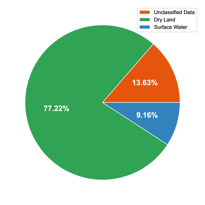
Figure 2: The percentage of total pixels that are marked as dry ($77.22\%$) or water ($9.18\%$) or which could not be classified by the labeling remote sensing analysts ($13.63\%$).

The first question to answer, given this high-quality labeled data, is how the distribution of the Sen1Floods11 dataset looks like. As depicted in Figure 2, only a small fraction of the hand-labeled dataset consists of flooded pixels.

This tail distribution is problematic, as a classifier trained on such a dataset will tend towards learning solutions, that prefer classifying something as dry land instead of as flooded. However, the resulting low Recall classifiers are undesirable, especially in the context of emergency-relief operations, as omitting certain regions from the flood inundation map may result in life losses.

Therefore strategies, which are mainly based on re-weighting the individual classes within the optimization objective of the given algorithm, have been proposed in flood mapping literature and shown their success at improving the mapping performance (Chini et al. (2017); Shaeri Karimi et al. (2019); Bai et al. (2021)). However, as we will observe in Section 4.3, for our tested classical machine learning approaches, this is not always beneficial.

3.3.2 Spatial Distribution

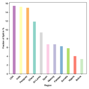
Figure 3: Spatial distribution of the Sen1Floods11 dataset per-country depicted as the relative area of each region of the complete hand-labeled Sen1Floods11 dataset.

Further insights can be gained by inspecting statistics for the individual regions in the Sen1Floods11 dataset. In Figure 3, a strong region-imbalance can be observed. Whilst images from the USA take up almost $16\%$ of the hand-labeled dataset, only very few images originating from Nigeria are present.

This can have an effect on the calculation of metrics, where a good performance of a flood mapping model on the majority regions, can result in overestimation of the true performance of the model in a global context. Moreover, algorithms trained on this dataset with the given bias, may learn to neglect minority areas. Thus constructing flood mapping algorithms on this dataset, that are agnostic to the region they operate on, is hard to achieve. We therefore specifically analyze our model using a novel metric calculation procedure, to ensure a good performance of the proposed classifier all around the world. To the best of our knowledge such an analysis has not been carried out for the Sen1Floods11 dataset, even though as is shown in Section 5.1, models such as the proposed GBDT-classifier can learn this bias.

4 Methodology

To analyze the performance of machine learning models on the Sen1Floods11 dataset, in the following Section 4.1 we explain our evaluation metrics and experiment setup. We then describe the features and their combinations, referred to as feature spaces, which have been explored in this work in Section 4.2. Lastly, we describe the evaluated models and their hyperparameter optimization in Section 4.3, before performing a quantitative and qualitative evaluation of the tested algorithms on the described feature spaces in the Section 5.

4.1 Evaluation Methodology

Throughout our experiments we use the pre-defined 60:20:20 train-validation-test splits of the hand-labeled data provided by the authors of the Sen1Floods11 dataset. Models are trained solely using the hand-labeled train data, with further grid-search based hyperparameter optimization using metrics as calculated on the validation split and averaged over four seeds, to avoid biasing the test set results (Deisenroth et al. (2020)). This helps to provide a fair comparison of the classical machine-learning algorithms with state-of-the-art neural network based approaches, despite these having a much larger model capacity.

In addition to comparative plots generated from these validation set results, we provide final evaluations using 16 seeds in tabular format for each of the different data-modalities that are available on the Sen1Floods11 dataset (SAR, optical and combined data) and present for each of these modalities the model according to the highest validation-set mean IoU.

Results on the additional Bolivia test split in the Sen1Floods11 dataset, containing data from a region that was not observed during training (Bonafilia et al. (2020)), are also provided in order to facilitate estimating the performance of the given algorithm on a new geographical location. Cross-validation procedures are not used to save processing time and make the tuning process more comparable to that of other past and future works utilizing the pre-defined splits.

4.1.1 Metrics

A commonly used metric for the evaluation of classifiers that intuitively represents the fraction of errors made by the classifier is Accuracy (ACC)(Bonafilia et al. (2020)), which is defined in terms of True Positives (TP), True Negatives (TN), False Positives (FP)and False Negatives (FN)for the surface water class in equation 1.

$$\text{\lx@glossaries@gls@link{acronym}{acc}{\leavevmode ACC}}=\frac{\text{\lx@glossaries@gls@link{acronym}{tp}{\leavevmode TP}}+\text{\lx@glossaries@gls@link{acronym}{tn}{\leavevmode TN}}}{\text{\lx@glossaries@gls@link{acronym}{tp}{\leavevmode TP}}+\text{\lx@glossaries@gls@link{acronym}{fp}{\leavevmode FP}}+\text{\lx@glossaries@gls@link{acronym}{tn}{\leavevmode TN}}+\text{\lx@glossaries@gls@link{acronym}{fn}{\leavevmode FN}}}$$ (1)

However, as pointed out by the authors of Sen1Floods11, Accuracy is not a good estimator of the performance of flood mapping classifiers (Bonafilia et al. (2020)) due to the class imbalance problem mentioned in Section 3.3.1. Substituting a classifier that predicts everything as dry land and the class distribution of Sen1Floods11 into equation 1 would still achieve an accuracy value of $\approx 89.4\%$.

In order to overcome this problem, Bonafilia et al. (2020) propose to use Intersection over Union (IoU) as the main metric for the Sen1Floods11 dataset.

$$\text{\lx@glossaries@gls@link{acronym}{iou}{\leavevmode IoU}}=\frac{\text{\lx@glossaries@gls@link{acronym}{tp}{\leavevmode TP}}}{\text{\lx@glossaries@gls@link{acronym}{tp}{\leavevmode TP}}+\text{\lx@glossaries@gls@link{acronym}{fp}{\leavevmode FP}}+\text{\lx@glossaries@gls@link{acronym}{fn}{\leavevmode FN}}}$$ (2)

Intuitively IoU describes the percentage of the area that is correctly identified as inundated (the intersection) out of the area that is actually water or has incorrectly been recognized as water (the union). Therefore it is unaffected by large portions of the images containing only dry land.

Konapala et al. (2021) base their evaluation on Precision (P), Recall (R), and $F_{1}$-Score ($F_{1}$). Recall hereby measures the percentage of inundated pixels that were recognized by the flood mapping algorithm, whereas Precision measures the fraction of pixels that have been correctly identified as water, out of all surface water classifications.

P $$=\frac{\text{\lx@glossaries@gls@link{acronym}{tp}{\leavevmode TP}}}{\text{\lx@glossaries@gls@link{acronym}{tp}{\leavevmode TP}}+\text{\lx@glossaries@gls@link{acronym}{fp}{\leavevmode FP}}}$$ (3)

R $$=\frac{\text{\lx@glossaries@gls@link{acronym}{tp}{\leavevmode TP}}}{\text{\lx@glossaries@gls@link{acronym}{tp}{\leavevmode TP}}+\text{\lx@glossaries@gls@link{acronym}{fn}{\leavevmode FN}}}$$ (4)

$$F_{1} =\frac{2\cdot\text{\lx@glossaries@gls@link{acronym}{pr}{\leavevmode P}}\cdot\text{\lx@glossaries@gls@link{acronym}{re}{\leavevmode R}}}{\text{\lx@glossaries@gls@link{acronym}{pr}{\leavevmode P}}+\text{\lx@glossaries@gls@link{acronym}{re}{\leavevmode R}}}=\frac{2\cdot\text{\lx@glossaries@gls@link{acronym}{tp}{\leavevmode TP}}}{2\cdot\text{\lx@glossaries@gls@link{acronym}{tp}{\leavevmode TP}}+\text{\lx@glossaries@gls@link{acronym}{fp}{\leavevmode FP}}+\text{\lx@glossaries@gls@link{acronym}{fn}{\leavevmode FN}}}$$ (5)

In addition to IoU, both Bonafilia et al. (2020) and Bai et al. (2021) also provide the Omission Error (OE) and Commission Error (CE) rates for the evaluated methods. These metrics represent how many pixels were incorrectly not recognized as inundated or dry land respectively. For these we define $\text{\lx@glossaries@gls@link{acronym}{tp}{\leavevmode TP}}_{\text{Dry}},\text{\lx@glossaries@gls@link{acronym}{fn}{\leavevmode FN}}_{\text{Dry}}$ as the True Positives and False Negatives rates for the dry land class, corresponding to TN and FP of the surface water class.

OE $$:=\frac{\text{\lx@glossaries@gls@link{acronym}{fn}{\leavevmode FN}}}{\text{\lx@glossaries@gls@link{acronym}{fn}{\leavevmode FN}}+\text{\lx@glossaries@gls@link{acronym}{tp}{\leavevmode TP}}}=\frac{\text{\lx@glossaries@gls@link{acronym}{fn}{\leavevmode FN}}+\text{\lx@glossaries@gls@link{acronym}{tp}{\leavevmode TP}}-\text{\lx@glossaries@gls@link{acronym}{tp}{\leavevmode TP}}}{\text{\lx@glossaries@gls@link{acronym}{fn}{\leavevmode FN}}+\text{\lx@glossaries@gls@link{acronym}{tp}{\leavevmode TP}}}=1-\text{\lx@glossaries@gls@link{acronym}{re}{\leavevmode R}}$$ (6)

CE $$:=\frac{\text{\lx@glossaries@gls@link{acronym}{fp}{\leavevmode FP}}}{\text{\lx@glossaries@gls@link{acronym}{fp}{\leavevmode FP}}+\text{\lx@glossaries@gls@link{acronym}{tn}{\leavevmode TN}}}=\frac{\text{\lx@glossaries@gls@link{acronym}{fn}{\leavevmode FN}}_{\text{Dry}}}{\text{\lx@glossaries@gls@link{acronym}{fn}{\leavevmode FN}}_{\text{Dry}}+\text{\lx@glossaries@gls@link{acronym}{tp}{\leavevmode TP}}_{\text{Dry}}}\stackrel{{\scriptstyle\ref{eq:classifiers:metrics:formulas:omission}}}{{=}}1-\text{\lx@glossaries@gls@link{acronym}{re}{\leavevmode R}}_{\text{Dry}}$$ (7)

It can be observed in equations 6 and 7 that the Ommission and Commission Error rates are equivalent to $1-$ the Recall of the flooded or dry land classes, respectively. Therefore, we only provide the equivalent Recall values instead of the Ommission and Commission Error rates, so that all metrics reported in this work consistently indicate better performance via larger values.

4.1.2 Reported Metrics and Metric Aggregation

It has to be noted that different ways of calculating the individual metrics are possible. Measures can be calculated for each of the images individually and then aggregated across the evaluation dataset, yielding a mean and standard deviation of the measure. Alternatively, classifiers can first aggregate errors from all images in the evaluation split by summing up the TP, TN, FP and FN values and evaluating the individual metric on the result, yielding just a single value. We will refer to metrics of the first kind as mean-based metrics and depict them for example as mean IoU, whereas metrics calculated using the second procedure will be called total metrics such as total IoU.

Accuracy and IoU are reported both as mean-based and total metrics, whilst $F_{1}$-Score, Recall, Precision of the surface water class and the Recall of the dry land class are reported only as total metrics. This provides us with insights into the stability of the algorithms performance across the evaluation split using the mean and standard deviation of the mean-based measures whilst also providing full error estimates using the total metrics as well as permitting comparisons with previous work carried out on the Sen1Floods11 dataset.

4.2 Tested Feature Spaces

To improve the quality of surface and flood water detection, many features based on optical data have been developed and used in the literature (McFEETERS (1996); Xu (2006); Feyisa et al. (2014)). Konapala et al. (2021) show that flood mapping approaches based on hand-crafted feature spaces can outperform those based on raw optical or SAR data (Konapala et al. (2021)). This Section, therefore, describes the used feature spaces and especially the transforms performed on optical satellite data.

A common method of analysis for remote sensing imagery based on multi-spectral instruments is the analysis of a corresponding remote sensing index (Huete (2012)). These indexes form simple and straight forward to implement functions of subsets of the available multi-spectral bands. For the detection of water, the Normalized Difference Water Index (NDWI) has been proposed (McFEETERS (1996)). This index is based upon surface water having a lower reflection in the NIR band, whilst at the same time producing a high reflection in the green bands (McFEETERS (1996)).

$$\text{\lx@glossaries@gls@link{acronym}{ndwi}{\leavevmode NDWI}}=\frac{\text{GREEN}-\text{\lx@glossaries@gls@link{acronym}{nir}{\leavevmode NIR}}}{\text{GREEN}+\text{\lx@glossaries@gls@link{acronym}{nir}{\leavevmode NIR}}}$$ (8)

As remarked by Xu (2006), the NDWI is susceptible to overprediction in urban areas. By using the SWIR band, instead of the NIR one, this effect can be reduced (Xu (2006); Konapala et al. (2021)).

$$\text{\lx@glossaries@gls@link{acronym}{mndwi}{\leavevmode MNDWI}}=\frac{\text{GREEN}-\text{\lx@glossaries@gls@link{acronym}{swir}{\leavevmode SWIR}-1}}{\text{GREEN}+\text{\lx@glossaries@gls@link{acronym}{swir}{\leavevmode SWIR}-1}}$$ (9)

Another index considered by Konapala et al. (2021) is the Automated Water Extraction Index (AWEI) (Feyisa et al. (2014); Konapala et al. (2021)). This index is based upon an empirical analysis of satellite imagery in order to facilitate good separation of the water and non-water classes. In order to handle cloud shadows, Feyisa et al. (2014) also provide the Automated Water Extraction Index for Applications with Shadows (AWEISH).

$$\text{\lx@glossaries@gls@link{acronym}{awei}{\leavevmode AWEI}}= 4\cdot(\text{GREEN}-\text{\lx@glossaries@gls@link{acronym}{swir}{\leavevmode SWIR}-1})$$

$$-\frac{1}{4}(\text{\lx@glossaries@gls@link{acronym}{nir}{\leavevmode NIR}}+11\cdot\text{\lx@glossaries@gls@link{acronym}{swir}{\leavevmode SWIR}-2})$$ (10)

$$\text{\lx@glossaries@gls@link{acronym}{aweish}{\leavevmode AWEISH}}= \text{BLUE}+\frac{5}{2}\cdot\text{GREEN}$$

$$-\frac{3}{2}\cdot(\text{\lx@glossaries@gls@link{acronym}{nir}{\leavevmode NIR}}+\text{\lx@glossaries@gls@link{acronym}{swir}{\leavevmode SWIR}-1})-\frac{\text{\lx@glossaries@gls@link{acronym}{swir}{\leavevmode SWIR}-2}}{4}$$ (11)

As is also done by Konapala et al. (2021), the concatenation along the channel axis of NDWI and MNDWI is referred to as cNDWI. Similarly, cAWEI refers to the concatenation of AWEI and AWEISH.

Furthermore, the Hue Saturation Value (HSV)transformation Smith (1978), of the SWIR-2, NIR, and red channels are exceedingly successful at extracting surface water (Pekel et al. (2016); Konapala et al. (2021)). HSV separates the color and intensity information present in the input channels, which may be the reason for the success of this transformation as pointed out by Pekel et al. (2016). This feature space and its raw bands are referred to as HSV (O3) and O3 respectively.

Lastly some experiments are carried out on the following additional feature spaces:

• S2 consists of all Sentinel-2 channels, whereas OPT removes the three 60m resolution bands similar to Landuyt et al. (2020).

• RGB and RGBN consist of the raw Red, Green, Blue, and optionally Near-Infrared channels. Good results on these feature spaces would enable the use of the constructed flood mapping approaches on satellite constellations utilizing micro-satellites. Here, only a subset of the channels used by larger satellites such as Sentinel-2 is provided, but with very frequent observation of the ground surface. As a result, classifiers that could work sufficiently well with this feature space would be very suitable for emergency relief operations (Mateo-Garcia et al. (2021)).

• HSV (RGB) builds upon the idea of Pekel et al. that the HSV-color space transformation helps separate the color information necessary for flood detection from the absolute intensity values (Pekel et al. (2016)) and performs a traditional HSV decomposition on the RGB feature space.

Combinations of the used feature spaces are depicted by concatenating their names with a $+$ sign in between, similar to the notation used by Konapala et al. (2021). However for larger combinations, it can be hard to identify the use of different data sources, so that an additional $\_$ is used to separate optical and SAR features. For example the string “SAR$\_$HSV(O3)+cAWEI+cNDWI” refers to the channel axis concatenation of SAR-data with optical data, where the optical data is provided as the combination of the HSV (O3), cAWEI and cNDWI feature spaces.

To summarize, for the purpose of this paper, the following 23 feature spaces were selected to compare the individual classifiers:

• SAR data only feature spaces: SAR

• Optical data only feature spaces: OPT, O3, S2, RGB, RGBN, HSV(RGB), HSV(O3), cNDWI, cAWEI, cAWEI+cNDWI, HSV(O3)+cAWEI+cNDWI

• SAR and optical feature spaces: SAR$\_$OPT, SAR$\_$O3, SAR$\_$S2, SAR$\_$RGB, SAR$\_$RGBN, SAR$\_$HSV(RGB), SAR$\_$HSV(O3), SAR$\_$cNDWI, SAR$\_$cAWEI, SAR$\_$cAWEI+cNDWI, SAR$\_$HSV(O3)+cAWEI+cNDWI

4.3 Models

Table 2: Choices for the maximum number of leaves of GBDT for the tested feature spaces. The feature spaces are categorized by their dimensionality as higher-dimensional input features permit more-splits (and therefore more leaves) per tree.

Feature Spaces	Dimensionality	Choices for the maximum number of Leaves
SAR, cNDWI,cAWEI	2	2, 4
O3, RGB, HSV (RGB), HSV (O3)	3	4, 8
SAR $\_$cNDWI, SAR $\_$cAWEI, RGBN, cAWEI +cNDWI	4	4, 8, 16
SAR $\_$O3, SAR $\_$RGB, SAR $\_$HSV (RGB), SAR $\_$HSV (O3)	5	8, 16, 32
SAR $\_$RGB N, SAR $\_$cAWEI +cNDWI, HSV (O3)$\_$cAWEI +cNDWI	6-7	16, 32, 64
OPT, S2, SAR $\_$OPT, SAR $\_$S2, SAR $\_$HSV (O3)+cAWEI +cNDWI	$>7$	32, 64, 128

On these feature spaces, five classical machine learning models are evaluated. This includes a linear model trained with stochastic gradient descent, three Bayesian classifiers with different model assumptions and a gradient boosting model.

To enable a fair comparison of the individual classifiers, a grid-search based hyperparameter optimization was performed for each of these feature spaces. The following Section 4.3.1 therefore briefly explains the linear SGD model as well as the Bayesian classifiers and the hyperparameters considered in these models, before Section 4.3.2 explains the GBDT model in detail.

4.3.1 Linear and Bayesian Models

The linear model is sklearn’s SGDClassifier (Pedregosa et al. (2011)). This implements a linear model trained with non-batchwise stochastic gradient descent using a reduce on plateau learning rate schedule. Hyperparameters considered were loss, in the form of huber loss, logistic loss, or hinge loss (Hastie et al. (2009c)), the strength of $L_{2}$ regularisation $\alpha\in\big{\{}10^{-i}|i\in\{0,1,2,3,4\}\big{\}}$ and whether class re-balancing should be applied.

The considered bayesian classifiers are Gaussian Naive Bayes, Linear Discriminant Analysis (LDA)and Quadratic Discriminant Analysis (QDA), also in the form of implementations by the sklearn machine-learning package (Pedregosa et al. (2011)). All three models determine the posterior probability of a given class and feature vector by using Bayes Rule to compute it from the likelihood of the feature vector for that class and the computed class prior probability. The models differ here in their modeling assumptions for the likelihood of the features. Whilst Naive Bayes assumes that all features are independent of each other and accordingly uses univariate Gaussian distributions, LDA and QDA compute a multivariate Gaussian distribution for each class, with LDA using the same covariance matrix for all classes (Hastie et al. (2009b)).

The hyperparameters considered were the shrinkage $\rho\in\left\{\frac{i}{10}\big{|}i\in\{0,\dots,10\}\right\}$ for LDA and sklearns covariance regularisation parameter in the range $\{0.0,0.00001,0.0001,0.001,0.01,0.1,0.5,1,2,4,8,10\}$ for QDA. Note that naive bayes does not have any hyperparameters to tune.

We observe that for all models, performance is very stable across different choices of regularisation parameters. Interestingly, we observed that the best performance for the simple linear model decreased when applying class-rebalancing, despite the model being trained on a highly imbalanced dataset. For all models it was observed that the selection of the feature space is the most important parameter, as will be analyzed in detail for the best model (GBDT) in the following sections.

4.3.2 Gradient Boosted Decision Tree (GBDT)

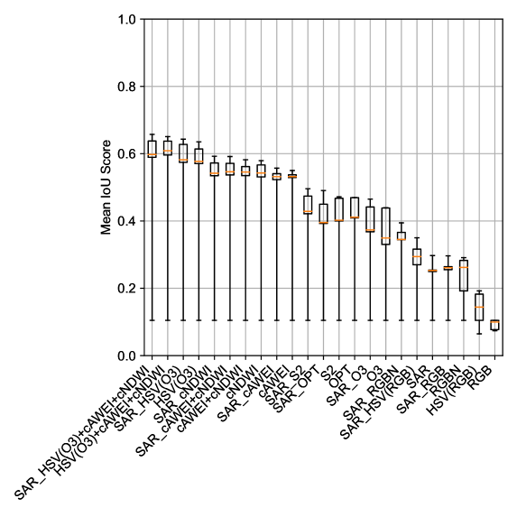
Figure 4: Influence of the used feature space on GBDT in terms of mean IoU on the Sen1Floods11 validation set. Each box represents the results for all evaluated hyperparameters of the corresponding feature space on the x-Axis, with results for the same hyperparmeter configuration being averaged over four seeds. The x-Axis is ordered by the respective max-values, with whiskers depicting the corresponding min-max ranges.

Table 3: Best results on the Sen1Floods11 test splits. The selected methods use both available data modalities, therefore Sentinel-1 (SAR) data and Sentinel-2 (optical) data. An extended version of this table, together with results on each modality separately, is provided in B. Metric values from related work on the Sen1Floods11 dataset are taken from the individual papers and, if available, ranked by total IoU and otherwise mean IoU within the evaluation split to compare them with the proposed classical machine learning approaches. The independently identically distributed (IID) split hereby refers to the regular Sen1Floods11 test set, whereas the domain shifted split refers to Bolivia test split. For each method, the used feature space as well as other parameter choices (such as hyperparameters or whether additional data has been used) are provided for a more in-depth comparison. Note that the reported standard deviation corresponds to the variation across the test set images, and not to the variation across individual runs with different seeds.

Test Split	Method	Feature Space	Mean IoU flooded (std)	Total IoU flooded	Mean Accuracy (std)	Total Accuracy	Total Precision flooded	Total Recall flooded	Total Recall dry	Total $F_{1}$-Score flooded	Parameter choices
IID Split	GBDT (ours)	SAR$\_$HSV(O3)+cAWEI+cNDWI	$\mathbf{0.7031}(\pm 0.2984)$	$\mathbf{0.8751}$	$\mathbf{0.9718}(\pm 0.1176)$	$\mathbf{0.9838}$	$\mathbf{0.9577}$	$0.9103$	$\mathbf{0.9943}$	$\mathbf{0.9334}$	$200$ trees
											up to $128$ leaves per tree
											regularisation $\lambda=1$
											learning rate: $0.1$
											subsample size: $262144$
	Naive Bayes (ours)	SAR$\_$HSV(O3)+cAWEI+cNDWI	$0.5187(\pm 0.3168)$	$0.7399$	$0.9522(\pm 0.0860)$	$0.9586$	$0.7784$	$\mathbf{0.9378}$	$0.9616$	$0.8503$	-
	Yadav et al. (2022)	SAR	-	$0.70$	-	-	-	-	-	0.83	Attentive Dual Stream Siamese Network
											Additional Pre-Flood SAR Data
	Bai et al. (2021)	SAR$\_$S2	$0.5873$	$0.6452$	$0.9338$	-	-	$0.6881$	$0.9884$	-	BASNet (Qin et al. (2019))
											Uses Sen1Floods11 weakly-labeled split for pretraining (4384 images)
Domain Shifted Split	GBDT (ours)	SAR$\_$HSV(O3)+cAWEI+cNDWI	$\mathbf{0.6070}(\pm 0.3542)$	$\mathbf{0.8357}$	$\mathbf{0.9705}(\pm 0.0293)$	$\mathbf{0.9730}$	$\mathbf{0.9584}$	$0.8671$	$\mathbf{0.9929}$	$\mathbf{0.9105}$	$200$ trees
											up to $128$ leaves per tree
											regularisation $\lambda=1$
											learning rate: $0.1$
											subsample size: $262144$
	Bai et al. (2021)	SAR$\_$S2	$0.5407$	$0.7890$	$0.9579$	-	-	$0.9234$	$0.9679$	-	BASNet (Qin et al. (2019))
											Uses Sen1Floods11 weakly-labeled split for pretraining (4384 images)
	Naive Bayes (ours)	SAR$\_$HSV(O3)+cAWEI+cNDWI	$0.4402(\pm 0.2889)$	$0.6160$	$0.8984(\pm 0.0776)$	$0.9033$	$0.6268$	$\mathbf{0.9728}$	$0.8902$	$0.7620$	-

Random forest or gradient boosting based models have been applied effectively for flood inundation mapping before (Lee et al. (2017); Feng et al. (2015); de la Cruz et al. (2020)). Gradient boosting is a steepest-descent ensemble learning method, fitting a model $f(x)$ of $M$ weak base learners $b$ (characterized by input $\mathbf{x}$ and parameters $\gamma_{m},1\leq m\leq M$) to form an additive function with expansion coefficients $\beta_{m},1\leq m\leq M$ (Hastie et al. (2009a)):

$$f(\mathbf{x})=\sum\limits_{m=1}^{M}\beta_{m}b(\mathbf{x},\gamma_{m})$$ (12)

In our case, only decision trees are considered as weak learners $b$ due to their good performance on other remote sensing tasks, to form the Gradient Boosted Decision Tree model. It is left to future work, to consider other valid weak learners, such as support vector machines (Hastie et al. (2009a); Friedman (2001)).

To fit the model in equation 12, the optimization problem in equation 13 has to be solved for a given loss function $\ell$, which is rarely feasible in practice:

$$\operatorname*{arg\,min}_{\begin{subarray}{c}\beta_{1},\dots,\beta_{M}\\ \gamma_{1},\dots,\gamma_{M}\end{subarray}}\sum_{i=1}^{N}\ell\left(y_{i},\sum_{m=1}^{M}\beta_{m}b(\mathbf{x_{i}},\gamma_{m})\right)$$ (13)

Instead “Forward Stagewise Additive Modeling” is performed, which approximates this solution by fitting the base learners sequentially, leaving the parameters of earlier learners unmodified (Hastie et al. (2009a)). It can be shown, that the optimal choice of parameters for model $m$ corresponds to the closest fit to the negative gradient of model $m-1$ to the loss $\ell$ (Friedman (2001)), resulting in the name “gradient boosting”.

As gradient boosting implementation, the highly-scalable implementation provided by LightGBM (Ke et al. (2017)) is used, which fits leaf-wise grown decision trees as weak base learners. Hereby all current leaves are considered as expansion candidates in each tree-building step, whereas traditional level-wise expansions first expand all nodes in each level, before considering leaves from the next level (Shi (2007); lightgbm-team (2022)). This allows for fewer nodes per-tree to achieve a given accuracy, at the cost of potentially causing over-fitting if the number of data points is small, however as there are more than $50M$ pixels in the hand-labeled training-set this is highly unlikely.

As is also pointed out by the LightGBM documentation, the number of boosting iterations performed and the number of leaves per tree are therefore very important parameters to tune. Higher values for both, allow the ensemble to better fit the training set, but may cause overfitting (lightgbm-team (2022); laurae (2018)). As expected, increasing the number of boosting iterations performed (and therefore the number of trees in the model), does improve performance, however this effect is rather insignificant and there are diminishing returns.

LightGBM also offers class re-balancing for training the forests, but similar to the linear SGD model, this does not improve the performance. Instead we can only observe a smaller Inter Quartile Range (IQR)and value range, indicating that the model is more stable with respect to the tested hyper-parameters, but does not converge towards the best solution achievable without re-balancing. We provide additional figures, depicting both effects, in A.

Due to the individual feature spaces varying in dimensionality ($2\leq d\leq 15$), deeper trees (trees with more nodes) are better suited to some feature spaces, than to others. Therefore the number of maximum leaves to test was hand-selected depending on the dimensionality as given in Table 2. Therefore, it is of higher interest to inspect the corresponding feature spaces, than the number of leaves used.

5 Results

The Feature Space is the single most important parameter to tune. This is shown in Figure 4, which depicts the performance of the classifier in terms of mean IoU with respect to the choice of the feature space. We find that the best feature space (SAR$\_$HSV(O3)+cAWEI+cNDWI), significantly outperforms the worst feature space (RGB) with a validation set mean IoU of $0.6574$ over $0.1047$. Similar differences could be observed for the other considered machine learning classifiers on their respective best and worst performing feature spaces, which can be found in A.

Furthermore, the hand-crafted feature spaces consistently outperform band combinations made up only of raw Sentinel-1 or Sentinel-2 data (S2, RGB, SAR, …). All feature spaces containing transformations appear before the raw band combinations in the ranking of Figure 4. Additionally, we find that the GBDT model is able to utilize multiple modalities as long as the features are of sufficient quality. The models using both SAR and optical data always outperform those trained on optical or SAR data only. Accordingly, GBDT models can also provide successful baselines if additional modalities become available on the Sen1Floods11 dataset.

However, the performance of the considered machine learning models using only SAR or RGB-data is far from enabling a satisfactory detection of flooded surface water. Although the HSV-transformation of the red, green and blue bands proposed in Section 4.2 is helpful, the observed performance is still unsatisfactory. To achieve a successful delineation of flooded areas, the multispectral channels of Sentinel-2 are essential.

5.1 Quantitative Analysis

Table 4: Statistics of per-region total metrics, calculated for the GBDT classifier on the Sen1Floods11 test set. In order to provide an estimate of the GBDT-model’s performance on regions all around the world, mean, standard deviation, value range and median of the per-region evaluations on the Sen1Floods11 test set are reported.

Feature Space	Statistic	ACC	IoU	$F_{1}$-Score	Precision	Recall
SAR $\_$HSV(O3)+cAWEI+cNDWI	Mean (std.)	$\mathbf{0.9857}(\pm 0.0125)$	$\mathbf{0.7998}(\pm 0.1750)$	$\mathbf{0.8788}(\pm 0.1141)$	$0.9372(\pm 0.0626)$	$\mathbf{0.8404}(\pm 0.1673)$
	Min-Max	$\mathbf{0.9612-0.9972}$	$\mathbf{0.5468-0.9713}$	$\mathbf{0.7070-0.9855}$	$0.7829-0.9880$	$\mathbf{0.5618-0.9832}$
	Median	$\mathbf{0.9912}$	$\mathbf{0.8888}$	$\mathbf{0.9410}$	$0.9561$	$\mathbf{0.9189}$
HSV(O3)+cAWEI+cNDWI	Mean (std.)	$0.9856(\pm 0.0125)$	$0.7925(\pm 0.1876)$	$0.8723(\pm 0.1261)$	$\mathbf{0.9406(\pm 0.0581)}$	$0.8311(0.1844)$
	Min-Max	$0.9616-0.9968$	$0.4684-0.9754$	$0.6380-0.9876$	$\mathbf{0.8035-0.9920}$	$0.4749-0.9832$
	Median	$0.9910$	$0.8860$	$0.9394$	$\mathbf{0.9647}$	$0.9162$
SAR	Mean (std.)	$0.9317(\pm 0.0432)$	$0.4054(\pm 0.1960)$	$0.5517(\pm 0.2019)$	$0.7569(\pm 0.2529)$	$0.4883(\pm 0.2013)$
	Min-Max	$0.8448-0.9928$	$0.1457-0.6819$	$0.2544-0.8109$	$0.2527-0.9775$	$0.1531-0.6928$
	Median	$0.9409$	$0.3912$	$0.5622$	$0.8215$	$0.5375$

To allow for a quantitative comparison with related work, Table 3 shows the test and bolivia test set, described in Section 4.1, results of the evaluated GBDT model and the naive bayes classifier combined SAR and optical data. Additional results of all tested models and evaluations using both data modalities individually are provided in B. The depicted methodologies were selected on the validation set primarily according to their mean IoU score, with the other metrics functioning as tie breakers in the order they appear in the table.

All considered classifiers outperform previous state-of-the-art neural network based approaches on the Sen1Floods11 test set in terms of total IoU, if multispectral data is available. We find that the selected GBDT model consistently outperforms all other methods for all metrics, with the exception of total Recall, for which the Naive Bayes classifier consistently performs best. GBDT achieves a test set mean and total IoU of $0.7010$ and $0.8767$ using optical data alone and $0.7031$, $0.8751$ using both optical and SAR data.

As mentioned previously in Section 2.2, Yadav et al. (2022) provide the current best total IoU of $0.70$ on the Sen1Floods11 dataset. Whilst they do not provide mean IoU values to compare to, it is observed in Table 3, that the GBDT model exceeds this with an improvement of $0.1751$ and $25.01\%$ in absolute and relative terms.

However, it has to be noted that both models use different datasources. Whereas our GBDT model uses optical and SAR post-flood data, Yadav et al. (2022) use pre-flood and post-flood SAR-Data to perform change detection, so that a comparison of both methods is hard. The best-performing approach using the same data sources as our model, though with more training data, is the approach by Bai et al. (2021). Our GBDT model exceeds this methodology in terms of mean and total IoU with a relative improvement of $19.7\%$ and $35.63\%$.

The previously reported neural network based models only exceed GBDT for the flooded Recall on the bolivia test set. This is due to the BASNet used by Bai et al. (2021) achieving an OE of $0.0766$ which corresponds to a flooded Recall of $0.9234$, which is larger than the $0.8671$ achieved by GBDT. On the other hand, in terms of flooded Recall the naive bayes classifier consistently outperforms all other methods, including the approach by Bai et al. (2021), thereby showing that for a suitable choice of feature space and classical machine learning method, the state-of-the-art neural network based approaches can be exceeded.

In general, the tested models tend to perform worse on the Bolivia test set, than on the regular test set. The only exception to this, is the linear model trained with SGD for SAR data that achieves a mean IoU of $0.4202$ on the Bolivia test set whilst achieving a mean IoU of $0.2597$ on the regular test set. This is a particularly surprising result, as all considered methodologies do not achieve a satisfying performance using SAR-only data on the test set. Here the best observed result is again the GBDT model with a mean IoU of $0.2880$ with the second best being the linear model.

The models do not perform very consistent across the individual regions. This is already indicated by the difference between the test and bolivia test sets, however to further analyze this effect, the standard deviation for mean-based metrics across the evaluation datasets was inspected as well and is presented in Table 3. We find that the GBDT-model exhibits a very large standard deviation so that it is likely that there are some images with very low IoU values. Furthermore, we find that for the other models the $2\sigma$ interval of the gaussian distribution given by the sample mean and standard deviation across the IoU s calculated for the individual images includes an IoU of $0$, as is shown in B.

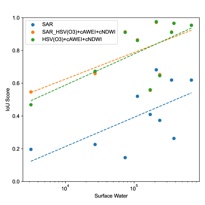
(a) Total IoU for the surface water class

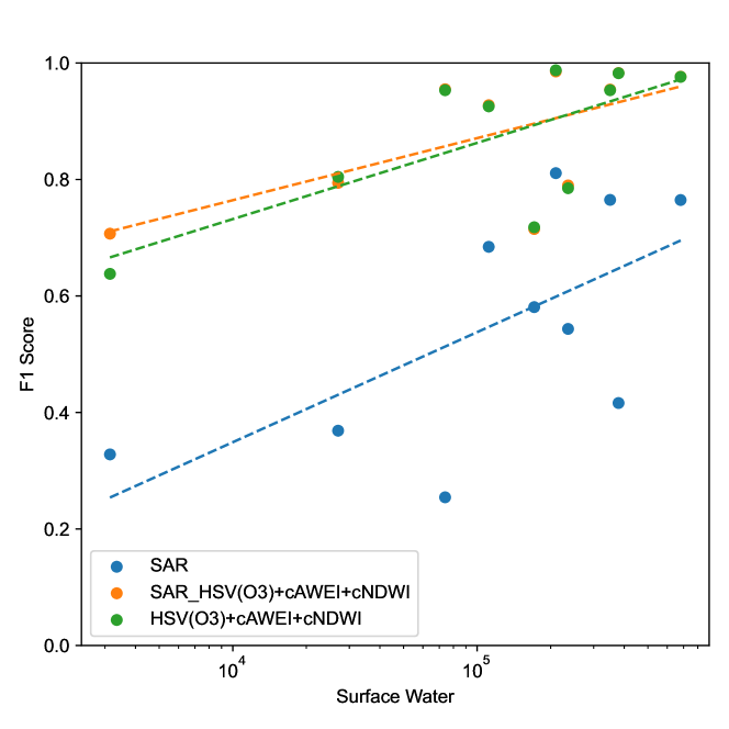
(b) Total $F_{1}$-Score for the surface water class

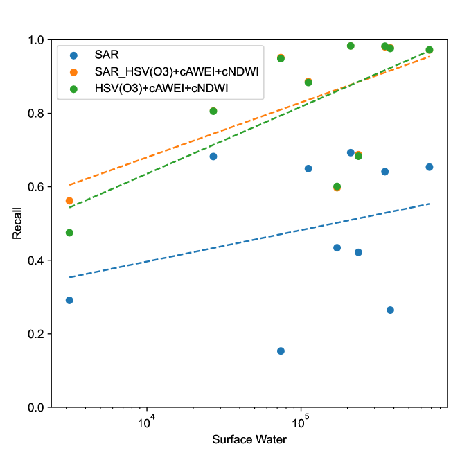
(c) Total Recall for the surface water class

Figure 5: Total region-wise metrics for the GBDT-model plotted as scatter plots. The amount of flooded pixels in the regions is depicted on the log-scale x-axis and the corresponding metric is depicted on the y-axis. Additionally, for each model a regression line is plotted to depict the trend present in the data.

Due to region imbalance, it is difficult to achieve a good estimate of the actual performance of the classifier on arbitrary regions of the world. For instance, mean-based metrics are biased with respect to majority regions, while total metrics such as total IoU favor regions with a larger representation of the minority class. Konapala et al. (2021) propose a regionwise cross-validation approach as an alternative evaluation methodology, where the model is trained ten times on nine of the eleven regions in the Sen1Floods11 dataset and then evaluated on the other two regions using total metrics. However, this does not solve the region imbalance problem as the two tested regions may be of varying size and furthermore does not allow estimating the performance of the classifier on in-distribution samples, thus requiring a different evaluation metric.

To further analyze the performance of the model on a global scale, we therefore propose to use total metrics that are calculated per-region for the selected GBDT classifiers. Plotting the so created metrics on a log-scale axis for the number of water pixels within each region, we can observe that for IoU, $F_{1}$-Score and Recall a clear trend is present for the model on all three data modalities. In regions with a larger number of water pixels, the models perform better for the flooded class as shown in Figures 5(a), 5(b), and 5(c). Whilst for Precision of the SAR GBDT-model the trend is also visible, we cannot observe it there for the other data modalities.

There exists a correlation between the amount of water pixels in a region and the classifiers performance. To verify this statement, the python sci-analysis package (Morrow, Chris (2019)) was used for performing statistical significance tests using the Spearman or Pearson Correlation Coefficients as appropriate. We find statistically significant (p-value $<0.05$) correlations for IoU and $F_{1}$-Score of the optical data only model and for $F_{1}$-Score and Precision using the SAR data only model. Furthermore, only Accuracy and Precision result in p-values greater than $0.09$ for the optical data based models, indicating that even for the remaining metrics, a bias towards majority regions is present.

GBDT performs well all around the world, despite the regional bias. We propose to use the mean and standard deviation of the total regionwise metrics, to allow a final quantitative evaluation of the classifier in a global context, independent of the region imbalance of the Sen1Floods11 dataset. The so calculated mean IoU value of $0.7998$ hereby serves as an estimate of the performance of the classifier, whilst the standard deviation of $0.1750$ permits an analysis of the performance on regions all around the world. Due to the aforementioned statistically significant bias present in the model, we additionally provide the value range and median in Table 4. With IoU values ranging from $0.5468$ to $0.9713$, we conclude that GBDT can provide high-quality flood inundation maps all around the world.

5.2 Qualitative Analysis

(a) Image from India

(b) Image from India

(c) Image from Ghana

(d) Image from Ghana

(e) Image from Paraguay

(f) Image from the USA

Figure 6: Failure cases of the GBDT-model for differing meteorological and geographical conditions. Areas marked in blue correspond to correct flood predictions, whereas magenta and green correspond to False Negatives and False Positives respectively.

(a) Image from Nigeria

(b) Image from India

(c) Image from India

(d) Image from Paraguay

(e) Image from Paraguay

(f) Image from Sri-Lanka

Figure 7: Positive examples of the GBDT-model for differing meteorological and geographical conditions. Areas marked in blue correspond to correct flood predictions, whereas magenta and green correspond to False Negatives and False Positives respectively.

Clouds negatively impact the performance of GBDT. Positive and negative cases of the GBDT model are inspected for a qualitative analysis of the performance of the optical data based GBDT-classifier on the Sen1Floods11 test set. As expected from a model that is mainly based on optical data, the first observation that can be made is that clouds negatively affect the resulting performance. Figure 6(a) shows that the forest-based classifier tends to erroneously predict areas affected by cloud shadows as flooded. Furthermore, in some images the classifier misses smaller riverbeds (Figures 6(b), 6(d), 6(e), 6(f)) or in one case even large parts of a connected water segment (Figure 6(c)). However, as is already shown by the high mean IoU, these errors are rare.

Presumably, the cause for the misclassification under cloudy conditions, is that the classifier operates on a pixel-wise basis. Figure 7(a) shows that the classifier is in principle capable of correctly recognizing dry land that is obscured by cloud shadows. However, for some objects on the ground, pixels may look identical under cloudy conditions to water pixels in other areas, so that the classifier cannot correctly identify them as dry land as it is missing the information of a cloud being close by. In this context, a windowed approach might be able to achieve better results. Alternatively, one could potentially overcome this limitation by adding the cloud shadow masks calculated for Sentinel-2 imagery by the Copernicus services and providing them as an additional input to the GBDT model.

In a similar sense, the sometimes missed features are likely caused by the model being trained on the complete dataset and not in a batch-wise manner. In contrast to neural-network based approaches, that are usually trained via minibatch-SGD and therefore are required to perform well on very different kinds of images to be able to reduce the training loss, the GBDT-model always observes pixels from all images in the dataset during training. Therefore, the model can learn to neglect some images in the dataset, that then might result in the mentioned negative samples.

In order to improve on these results, it may therefore be an interesting direction for future work to explore the potential of training the GBDT-model in a batched way as well, thereby leveraging the same regularisation effect. This procedure, in combination with for example a region-stratified sampling of batches, might also benefit the stability of the algorithm with respect to different regions around the world.

GBDT provides highly precise segmentation maps. This can be verified by inspecting the positive samples in Figure 7 which show the good performance also reported by the metrics. Images with large flooded areas, such as depicted in Figures 7(c), 7(b), and 7(d), can be segmented almost completely correct as well as images with only small, mostly disconnected flooded areas as shown in Figures 7(e) and 7(f).

It should be noted, that especially the latter is an advantage of this pixel-based approach over reported neural-network based image segmentation methods, as neural-networks often produce blurry boundaries or miss smaller features in the resulting segmentation map (Valanarasu et al. (2021); Bai et al. (2021)), which was not observed for the GBDT-model.

6 Conclusions and Future Work

In this work, the potential of five classical machine learning models as pixel-wise classifiers for flood inundation mapping has been systematically investigated. Quantitative analysis based on an exhaustive hyperparameter search for 23 feature spaces each shows that all classical machine learning algorithms can outperform current state-of-the-art deep learning approaches in terms of total IoU with a relative improvement of up to $25.01\%$. Furthermore, a qualtitative analysis shows that the best-performing model, a pixel-wise Gradient Boosted Decision Tree classifier, enables highly accurate segmentation bounds with an accuracy that is outperforming all previous convolutional filter-based neural networks.

Our analysis also shows that the GBDT model learns a bias with respect to regions with a greater presence of the surface water minority class. While this bias is not as pronounced as an initial examination of the standard deviation across the images of the test dataset would suggest, a trend can still be seen visually and was verified using statistical tests. Due to the observed region imbalance of the Sen1Floods11 dataset, we additionally propose to calculate regionwise total metrics to enable unbiased evaluations in a global context. The GBDT model hereby achieves a regionwise mean IoU of $0.7998$ and whilst we cannot compare this to existing work yet, we make our code available so that future research can easily employ unbiased regionwise total evaluations as well as using our proposed feature spaces.

It should be noted that in this paper, the GBDT model was only used to detect surface water during flooding, and no distinction was made between permanent water surfaces and flooded areas. However, since maps of permanent water are freely available (Bonafilia et al. (2020)), this is not a limitation in practice, since permanent water regions such as lakes or rivers can simply be subtracted from the surface water mask to obtain a map of pure flooded areas. Accordingly, the proposed model is also suitable for the detection of pure flooded areas.

Additionally, the success of such a simple pixel-wise model on optical data shows that, using the right feature space, little contextual information is needed to enable very accurate flood detection. Accordingly, methodologies using specialized architectures for precise segmentation of images, such as BASNet (Qin et al. (2019)) which is used by Bai et al. (2021), are expected to be particularly successful provided optical data is available. However, this is also a potential challenge for future deep data fusion approaches using optical data, as the deep neural networks used may be inclined to rely solely on the high predictive capability of optical data without using the other modalities effectively.

Lastly, while the proposed cassical machine learning models are already very well suited as standalone flood mapping classifiers, further interesting directions for future work emerge from the interaction with Deep Learning. For all algorithms it could be observed that the performance of the respective classifier strongly depends on the feature space used. ML models based on multispectral data outperform those based on only RGB or SAR data by a multiple. However, these feature spaces exhibit useful properties such as higher revisit-times or independence from weather conditions (Shen et al. (2019); Mateo-Garcia et al. (2021)) making them highly desirable flood mapping feature spaces. Since prior work has shown that deep learning models based on larger datasets with weak labels can outperform those based on smaller datasets, albeit higher quality labels (Katiyar et al. (2021); Bonafilia et al. (2020)), further research could therefore analyze the potential of the described ML algorithms as label-sources for deep learning methodologies trained in a global context based on these more challenging feature spaces.

We believe that a classifier, which outperforms the previous state-of-the-art results in terms of mean IoU, total IoU and mean Accuracy with values of $0.7031$, $0.8751$ and $0.9718$ compared to $0.5873$, $0.70$ and $0.9338$, will serve both as a highly accurate flood inundation mapping methodology and a label-source for the development of future deep learning based approaches.

Appendix A Further Hyperparameter Analysis

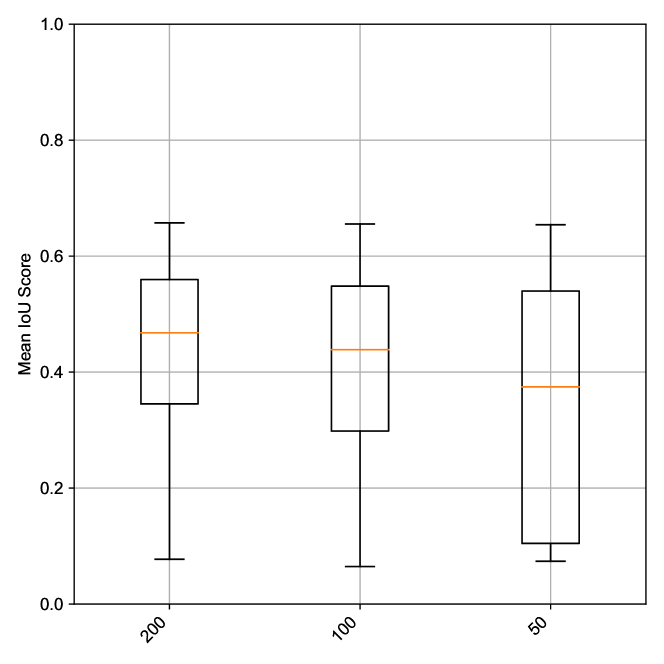
(a) Influence of the number of trees on GBDT

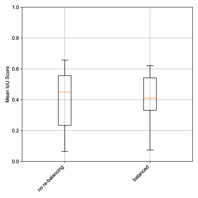
(b) Influence of class re-balancing on GBDT

Figure 8: Influence of tested parameters on GBDT in terms of mean IoU on the Sen1Floods11 validation set. The x-Axis is ordered by the respective max-values, with whiskers depicting the corresponding min-max ranges.

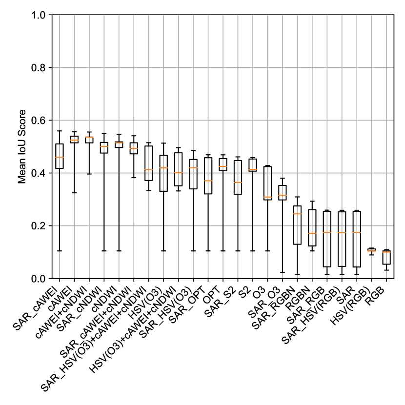
(a) Influence of the choice of feature space on the linear SGD model.

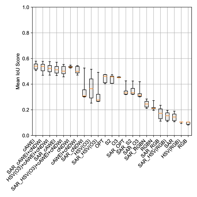
(b) Influence of the choice of feature space on Linear Discriminant Analysis (LDA).

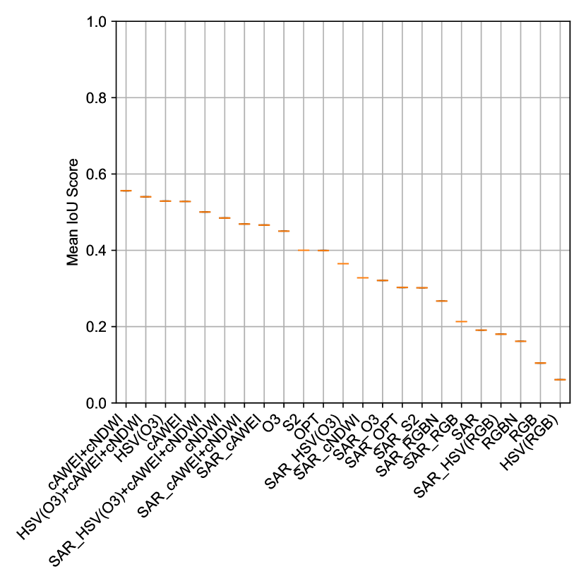
(c) Influence of the choice of feature space on the Naive Bayes classifier.

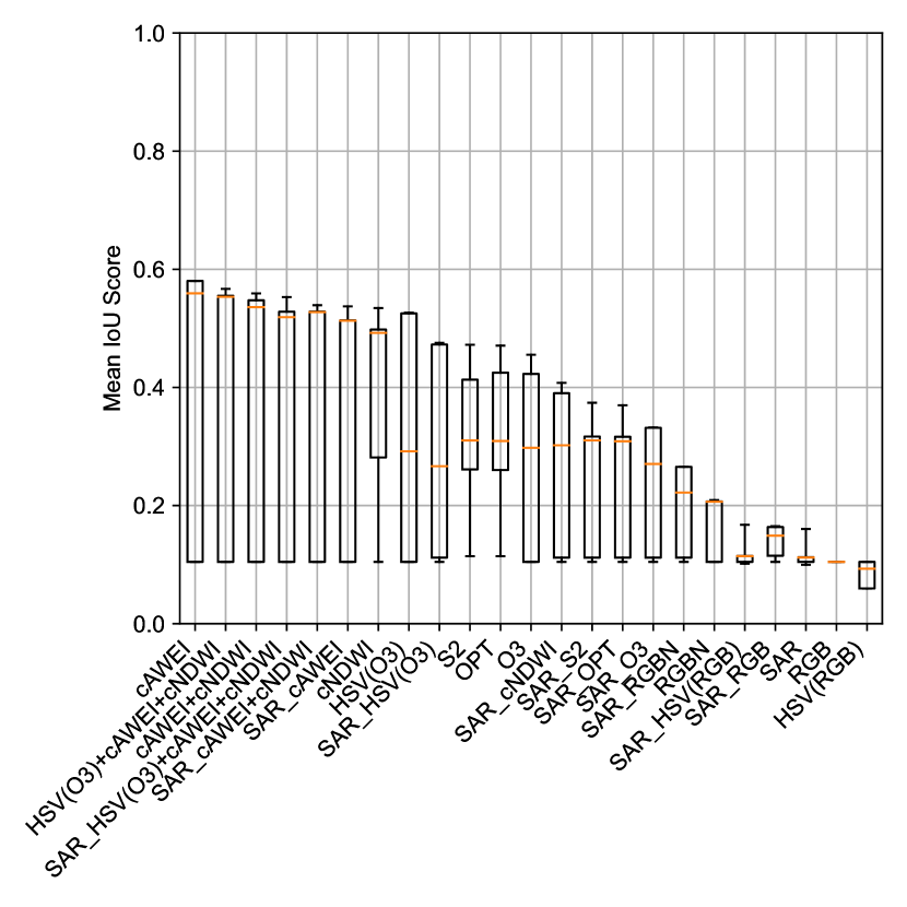
(d) Influence of the choice of feature space on Quadratic Discriminant Analysis (QDA).

Figure 9: Influence of the choice of feature space on the tested classical machine learning models besides GBDT in terms of mean IoU on the Sen1Floods11 validation set. Similar to Figure 4, the x-Axis is ordered by the respective max-values, with whiskers depicting the corresponding min-max ranges.

More details to the results of our hyperparameter search for GBDT can be found in Figure 8. Additionally, we observed that for all considered machine learning models, the feature space forms the most important parameter. This is depicted in Figure 9.

Appendix B Additional Quantitative Results

Table 5: Extended performance comparison of the proposed classifiers using both data modalities, therefore Sentinel-1 (SAR) data and Sentinel-2 (optical) data, with related work. Metric values from related work on the Sen1Floods11 dataset are taken from the individual papers and, if available, ranked by total IoU and otherwise mean IoU within the evaluation split to compare them with the proposed classical machine learning approaches. The independently identically distributed (IID) split hereby refers to the regular Sen1Floods11 test set, whereas the domain shifted split refers to Bolivia test split. For each method, the used feature space as well as other parameter choices (such as hyperparameters or whether additional data has been used) are provided for a more in-depth comparison. Note that the reported standard deviation corresponds to the variation across the test set images, and not to the variation across individual runs with different seeds.

Test Split	Method	Feature Space	Mean IoU flooded (std)	Total IoU flooded	Mean Accuracy (std)	Total Accuracy	Total Precision flooded	Total Recall flooded	Total Recall dry	Total $F_{1}$-Score flooded	Parameter choices
IID Split	GBDT	SAR$\_$HSV(O3)+cAWEI+cNDWI	$\mathbf{0.7031}(\pm 0.2984)$	$\mathbf{0.8751}$	$\mathbf{0.9718}(\pm 0.1176)$	$\mathbf{0.9838}$	$\mathbf{0.9577}$	$0.9103$	$\mathbf{0.9943}$	$\mathbf{0.9334}$	$200$ trees
											up to $128$ leaves per tree
											regularisation $\lambda=1$
											learning rate: $0.1$
											subsample size: $262144$
	Linear Model (SGD)	SAR$\_$HSV(O3)	$0.5701(\pm 0.3305)$	$0.7966$	$0.9627(\pm 0.1127)$	$0.9724$	$0.9172$	$0.8569$	$0.9889$	$0.8860$	logistic loss
											no class rebalancing
											regularisation $\alpha=0.0001$
	Linear Discriminant Analysis	SAR$\_$cAWEI+cNDWI	$0.5631(\pm 0.3262)$	$0.7828$	$0.9618(\pm 0.0906)$	$0.9685$	$0.8540$	$0.9048$	$0.9776$	$0.8780$	shrinkage $\rho=0.1$
	Quadratic Discriminant Analysis	SAR$\_$HSV(O3)+cAWEI+cNDWI	$0.5679(\pm 0.3232)$	$0.7695$	$0.9631(\pm 0.0654)$	$0.9653$	$0.8201$	$0.9258$	$0.9710$	$0.8698$	regularisation: $0$
	Naive Bayes	SAR$\_$HSV(O3)+cAWEI+cNDWI	$0.5187(\pm 0.3168)$	$0.7399$	$0.9522(\pm 0.0860)$	$0.9586$	$0.7784$	$\mathbf{0.9378}$	$0.9616$	$0.8503$	-
	Yadav et al. (2022)	SAR	-	$0.70$	-	-	-	-	-	0.83	Attentive Dual Stream Siamese Network
											Additional Pre-Flood SAR Data
	Jain et al. (2022)	SAR	-	$0.6871$	-	-	-	-	-	-	DeepLabV3+ (Chen et al. (2018))
											Multimodal contrastive pretraining
											1,087,502 additional unlabeled images
	Patel et al. (2021)	SAR	-	$0.6692$	-	-	-	-	-	-	DeepLabV3+ (Chen et al. (2018))
											SimCLR pretraining
											67k additional unlabeled images
	Bai et al. (2021)	SAR$\_$S2	$0.5873$	$0.6452$	$0.9338$	-	-	$0.6881$	$0.9884$	-	BASNet (Qin et al. (2019))
											Uses Sen1Floods11 weakly-labeled split for pretraining (4384 images)
	Katiyar et al. (2021)	SAR	$0.494$	-	-	-	-	$0.7958$	$0.9796$	-	U-Net (Ronneberger et al. (2015)) Uses Sen1Floods11 weakly-labeled split for pretraining (4384 images)
	Sentinel-2 Weak Bonafilia et al. (2020)	SAR	$0.4084$	-	$0.9384$	-	-	$0.7518$	$0.9222$	-	Resnet-50 (He et al. (2016))
											Uses Sen1Floods11 weakly-labeled split for pretraining (4384 images)
	Otsu-Reference Bonafilia et al. (2020)	SAR	$0.3591$	-	$0.9389$	-	-	$0.8573$	$0.9151$	-	VH-Threshold
	Sentinel-1 Weak Bonafilia et al. (2020)	SAR	$0.3092$	-	-	-	-	$0.8876$	$0.9003$	-	Resnet-50 (He et al. (2016))
											Uses Sen1Floods11 weakly-labeled split for pretraining (4384 images)
Domain Shifted Split	GBDT	SAR$\_$HSV(O3)+cAWEI+cNDWI	$\mathbf{0.6070}(\pm 0.3542)$	$\mathbf{0.8357}$	$\mathbf{0.9705}(\pm 0.0293)$	$\mathbf{0.9730}$	$\mathbf{0.9584}$	$0.8671$	$\mathbf{0.9929}$	$\mathbf{0.9105}$	$200$ trees
											up to $128$ leaves per tree
											regularisation $\lambda=1$
											learning rate: $0.1$
											subsample size: $262144$
	Linear Model (SGD)	SAR$\_$HSV(O3)	$0.5599(\pm 0.3231)$	$0.7900$	$0.9581(\pm 0.0382)$	$0.9615$	$0.8768$	$0.8925$	$0.9746$	$0.8820$	logistic loss
											regularisation $\alpha=0.0001$
											no class rebalancing
	Bai et al. (2021)	SAR$\_$S2	$0.5407$	$0.7890$	$0.9579$	-	-	$0.9234$	$0.9679$	-	BASNet (Qin et al. (2019))
											Uses Sen1Floods11 weakly-labeled split for pretraining (4384 images)
	Patel et al. (2021)	SAR	-	$0.7156$	-	-	-	-	-	-	DeepLabV3+ (Chen et al. (2018))
											FixMatch pretraining
											67k additional unlabeled images
	Linear Discriminant Analysis	SAR$\_$cAWEI+cNDWI	$0.4881(\pm 0.2924)$	$0.6776$	$0.9196(\pm 0.0612)$	$0.9241$	$0.7027$	$0.9557$	$0.9181$	$0.8050$	shrinkage $\rho=0.1$
	Quadratic Discriminant Analysis	SAR$\_$HSV(O3)+cAWEI+cNDWI	$0.4485(\pm 0.2880)$	$0.6554$	$0.9163(\pm 0.0680)$	$0.9205$	$0.6789$	$0.9500$	$0.9150$	$0.7916$	regularisation: $0$
	Naive Bayes	SAR$\_$HSV(O3)+cAWEI+cNDWI	$0.4402(\pm 0.2889)$	$0.6160$	$0.8984(\pm 0.0776)$	$0.9033$	$0.6268$	$\mathbf{0.9728}$	$0.8902$	$0.7620$	-
	Sentinel-1 Weak Bonafilia et al. (2020)	SAR	$0.3871$	-	$0.9384$	-	-	$0.7213$	$0.9305$	-	Resnet-50 (He et al. (2016))
											Uses Sen1Floods11 weakly-labeled split for pretraining (4384 images)
	Otsu-Reference Bonafilia et al. (2020)	SAR	$0.3862$	-	-	-	-	$0.7520$	$0.9475$	-	VH-Threshold
	Sentinel-2 Weak Bonafilia et al. (2020)	SAR	$0.3160$	-	-	-	-	$0.8425$	$0.9586$	-	Resnet-50 (He et al. (2016))
											Uses Sen1Floods11 weakly-labeled split for pretraining (4384 images)

Table 6: Performance comparison of the best classifiers for each model using only Sentinel-2 (optical) data, in the same format as Table 5.

Test Split	Method	Feature Space	Mean IoU flooded (std)	Total IoU flooded	Mean Accuracy (std)	Total Accuracy	Total Precision flooded	Total Recall flooded	Total Recall dry	Total $F_{1}$-Score flooded	Parameter choices
IID Split	GBDT	HSV(O3)+cAWEI+cNDWI	$\mathbf{0.7010}(\pm 0.3001)$	$\mathbf{0.8767}$	$\mathbf{0.9719}(\pm 0.1170)$	$\mathbf{0.9839}$	$\mathbf{0.9568}$	$0.9129$	$\mathbf{0.9941}$	$\mathbf{0.9343}$	$200$ trees
											up to $64$ leaves per tree
											regularisation $\lambda=1$
											learning rate: $0.1$
											subsample size: $1048576$
	Linear Discriminant Analysis	cAWEI	$0.5928(\pm 0.3199)$	$0.8140$	$0.9621(\pm 0.1141)$	$0.9739$	$0.8819$	$0.9136$	$0.9825$	$0.8975$	shrinkage $\rho=0$
	Quadratic Discriminant Analysis	cAWEI	$0.5880(\pm 0.3211)$	$0.8139$	$0.9622(\pm 0.1150)$	$0.9740$	$0.8849$	$0.9104$	$0.9831$	$0.8974$	regularisation: $0.001$
	Linear Model (SGD)	HSV(O3)	$0.5742(\pm 0.3336)$	$0.7908$	$0.9612(\pm 0.1160)$	$0.9712$	$0.9104$	$0.8547$	$0.9879$	$0.8816$	logistic loss
											regularisation $\alpha=0.0001$
											no class rebalancing
	Naive Bayes	cAWEI+cNDWI	$0.5511(\pm 0.3177)$	$0.7343$	$0.9551(\pm 0.0636)$	$0.9574$	$0.7692$	$\mathbf{0.9418}$	$0.9596$	$0.8468$	-
Domain Shifted Split	GBDT	HSV(O3)+cAWEI+cNDWI	$\mathbf{0.6006}(\pm 0.3537)$	$\mathbf{0.8295}$	$0.9692(\pm 0.0312)$	$0.9719$	$\mathbf{0.9571}$	$0.8616$	$\mathbf{0.9927}$	$\mathbf{0.9068}$	$200$ trees
											up to $64$ leaves per tree
											regularisation $\lambda=1$
											learning rate: $0.1$
											subsample size: $1048576$
	Quadratic Discriminant Analysis	cAWEI	$0.5804(\pm 0.3350)$	$0.7996$	$\mathbf{0.9739}(\pm 0.0355)$	$\mathbf{0.9748}$	$0.8676$	$0.9107$	$0.9828$	$0.8886$	regularisation: $0.001$
	Linear Model (SGD)	HSV(O3)	$0.5458(\pm 0.3135)$	$0.7796$	$0.9551(\pm 0.0379)$	$0.9585$	$0.8649$	$0.8936$	$0.9707$	$0.8750$	logistic loss
											regularisation $\alpha=0.0001$
											no class rebalancing
	Linear Discriminant Analysis	cAWEI	$0.5394(\pm 0.2922)$	$0.7451$	$0.9436(\pm 0.0533)$	$0.9482$	$0.7730$	$0.9537$	$0.9472$	$0.8539$	shrinkage $\rho=0$
	Naive Bayes	cAWEI+cNDWI	$0.4410(\pm 0.2877)$	$0.6290$	$0.9039(\pm 0.0741)$	$0.9089$	$0.6400$	$\mathbf{0.9735}$	$0.8968$	$0.7723$	-

Table 7: Performance comparison of the best classifiers for each model using only Sentinel-1 (SAR) data, in the same format as Table 5.

Test Split	Method	Feature Space	Mean IoU flooded (std)	Total IoU flooded	Mean Accuracy (std)	Total Accuracy	Total Precision flooded	Total Recall flooded	Total Recall dry	Total $F_{1}$-Score flooded	Parameter choices
IID Split	Linear Model (SGD)	SAR	$0.2597(\pm 0.2834)$	$\mathbf{0.4968}$	$0.8964(\pm 0.1299)$	$0.9063$	$0.6022$	$\mathbf{0.7396}$	$0.9302$	$\mathbf{0.6639}$	hinge loss
											regularisation $\alpha=0.1$
											class rebalancing
	GBDT	SAR	$\mathbf{0.2880}(\pm 0.3179)$	$0.4713$	$\mathbf{0.9207}(\pm 0.1644)$	$\mathbf{0.9290}$	$\mathbf{0.8722}$	$0.5063$	$\mathbf{0.9894}$	$0.6407$	$50$ trees
											up to $2$ leaves per tree
											regularisation $\lambda=0.01$
											learning rate: $0.1$
											subsample size: $262144$
	Naive Bayes	SAR	$0.1852(\pm 0.2594)$	$0.4024$	$0.9064(\pm 0.1650)$	$0.9142$	$0.7571$	$0.4621$	$0.9788$	$0.5739$	-
	Linear Discriminant Analysis	SAR	$0.1837(\pm 0.2597)$	$0.3960$	$0.9057(\pm 0.1684)$	$0.9134$	$0.7568$	$0.4538$	$0.9791$	$0.5674$	shrinkage $\rho=1$
	Quadratic Discriminant Analysis	SAR	$0.1506(\pm 0.2335)$	$0.3345$	$0.8986(\pm 0.1745)$	$0.9058$	$0.7419$	$0.3785$	$0.9812$	$0.5013$	regularisation: $1$
Domain Shifted Split	Linear Model (SGD)	SAR	$\mathbf{0.4202}(\pm 0.3209)$	$\mathbf{0.6552}$	$0.9298(\pm 0.0607)$	$\mathbf{0.9328}$	$0.7791$	$\mathbf{0.8047}$	$0.9570$	$\mathbf{0.7917}$	hinge loss
											regularisation $\alpha=0.1$
											class rebalancing
	GBDT	SAR	$0.2842(\pm 0.2578)$	$0.4981$	$0.9127(\pm 0.0893)$	$0.9182$	$\mathbf{0.9487}$	$0.5119$	$\mathbf{0.9948}$	$0.6650$	$50$ trees
											up to $2$ leaves per tree
											regularisation $\lambda=0.01$
											learning rate: $0.1$
											subsample size: $262144$
	Naive Bayes	SAR	$0.1628(\pm 0.1527)$	$0.2683$	$0.8668(\pm 0.1389)$	$0.8731$	$0.7592$	$0.2933$	$0.9825$	$0.4231$	-
	Linear Discriminant Analysis	SAR	$0.1571(\pm 0.1476)$	$0.2531$	$0.8644(\pm 0.1434)$	$0.8706$	$0.7490$	$0.2766$	$0.9825$	$0.4040$	shrinkage $\rho=1$
	Quadratic Discriminant Analysis	SAR	$0.0665(\pm 0.0628)$	$0.0957$	$0.8354(\pm 0.1853)$	$0.8441$	$0.5441$	$0.1041$	$0.9836$	$0.1747$	regularisation: $1$

To provide a full quantitative analysis of the tested methodologies, Tables 5-7 extend Table 3. We depict the results for all tested methodologies on their best performing feature space in Table 5 alongside all prior work that, to the best of our knowledge, has so far been carried out on the Sen1Floods11 dataset. Tables 6 and 7 additionally show the results of the proposed machine learning approaches using only optical and SAR data respectively.

References

- Bai et al. (2021) Bai, Y., Wu, W., Yang, Z., Yu, J., Zhao, B., Liu, X., Yang, H., Mas, E., Koshimura, S., 2021. Enhancement of Detecting Permanent Water and Temporary Water in Flood Disasters by Fusing Sentinel-1 and Sentinel-2 Imagery Using Deep Learning Algorithms: Demonstration of Sen1Floods11 Benchmark Datasets. Remote Sensing 13, 2220. doi:10.3390/rs13112220.
- Banerjee et al. (2020) Banerjee, S., Chaudhuri, S.S., Mehra, R., Misra, A., 2020. A Comprehensive Survey on Frost Filter and its Proposed Variants, in: 2020 5th International Conference on Communication and Electronics Systems (ICCES), pp. 109–114. doi:10.1109/ICCES48766.2020.9137869.
- Bentivoglio et al. (2021) Bentivoglio, R., Isufi, E., Jonkman, S.N., Taormina, R., 2021. Deep Learning Methods for Flood Mapping: A Review of Existing Applications and Future Research Directions. Hydrology and Earth System Sciences Discussions , 1–43doi:10.5194/hess-2021-614.
- Bonafilia et al. (2020) Bonafilia, D., Tellman, B., Anderson, T., Issenberg, E., 2020. Sen1Floods11: A Georeferenced Dataset to Train and Test Deep Learning Flood Algorithms for Sentinel-1, in: Proceedings of the IEEE/CVF Conference on Computer Vision and Pattern Recognition Workshops, pp. 210–211.
- Brakenridge (2021) Brakenridge, G., 2021. Global active archive of large flood events. http://floodobservatory.colorado.edu/Archives/index.html. Last accessed: 2022-05-05.
- Chen et al. (2018) Chen, L.C., Zhu, Y., Papandreou, G., Schroff, F., Adam, H., 2018. Encoder-Decoder with Atrous Separable Convolution for Semantic Image Segmentation, in: Proceedings of the European Conference on Computer Vision (ECCV), pp. 801–818.
- Chen et al. (2020) Chen, T., Kornblith, S., Norouzi, M., Hinton, G., 2020. A Simple Framework for Contrastive Learning of Visual Representations, in: Proceedings of the 37th International Conference on Machine Learning, PMLR. pp. 1597–1607.
- Chini et al. (2017) Chini, M., Hostache, R., Giustarini, L., Matgen, P., 2017. A Hierarchical Split-Based Approach for Parametric Thresholding of SAR Images: Flood Inundation as a Test Case. IEEE Transactions on Geoscience and Remote Sensing 55, 6975–6988. doi:10.1109/TGRS.2017.2737664.
- de la Cruz et al. (2020) de la Cruz, R.M., Olfindo Jr., N.T., Felicen, M.M., Borlongan, N.J.B., Difuntorum, J.K.L., Marciano Jr., J.J.S., 2020. Near-Realtime Flood Detection From Multi-Temporal Sentinel Radar Images Using Artifical Intelligence. The International Archives of the Photogrammetry, Remote Sensing and Spatial Information Sciences XLIII-B3-2020, 1663–1670. doi:10.5194/isprs-archives-XLIII-B3-2020-1663-2020.
- Deisenroth et al. (2020) Deisenroth, M.P., Faisal, A.A., Ong, C.S., 2020. Mathematics for Machine Learning. Cambridge University Press.
- Díaz (2020) Díaz, A., 2020. Discover the 4 V’s of Big Data. Last Accessed:2022-05-19.
- Disaster (CRED) Disaster(CRED), 2015. The Human Cost Of Natural Disasters: A Global Perspective. Report. Centre for Research on the Epidemiology of Disaster(CRED).
- dpa,epa (2021) dpa,epa, Z., 2021. Hochwasser trifft bayern, sachsen und österreich - ZDFheute. https://www.zdf.de/nachrichten/panorama/hochwasser-unwetter-bayern-sachsen-oesterreich-100.html. Last accessed: 2022-05-05.
- Drakonakis et al. (2022) Drakonakis, G.I., Tsagkatakis, G., Fotiadou, K., Tsakalides, P., 2022. OmbriaNet—Supervised Flood Mapping via Convolutional Neural Networks Using Multitemporal Sentinel-1 and Sentinel-2 Data Fusion. IEEE Journal of Selected Topics in Applied Earth Observations and Remote Sensing 15, 2341–2356. doi:10.1109/JSTARS.2022.3155559.
- ESA (2022) ESA, 2022. About Copernicus — Copernicus. https://www.copernicus.eu/en/about-copernicus. Last accessed: 2022-05-05.
- ESA (2022) ESA, 2022. Sentinel-1 - missions - instrument payload - sentinel online. https://sentinels.copernicus.eu/web/sentinel/missions/sentinel-1/instrument-payload. Last accessed: 2022-05-05.
- ESA (2022a) ESA, 2022a. Sentinel-2 Technical Guide - MSI Instrument Overview. https://sentinels.copernicus.eu/web/sentinel/technical-guides/sentinel-2-msi/msi-instrument. Last accessed: 2022-05-05.
- ESA (2022b) ESA, 2022b. Sentinel-2 User Guide - MSI Overview. https://sentinels.copernicus.eu/web/sentinel/user-guides/sentinel-2-msi/overview. Last accessed: 2022-05-05.
- Everingham et al. (2014) Everingham, M., Eslami, S., Gool, L., Williams, C.K.I., Winn, J., Zisserman, A., 2014. The pascal visual object classes challenge: A retrospective. International Journal of Computer Vision 111, 98–136.
- Feng et al. (2015) Feng, Q., Gong, J., Liu, J., Li, Y., 2015. Flood Mapping Based on Multiple Endmember Spectral Mixture Analysis and Random Forest Classifier—The Case of Yuyao, China. Remote Sensing 7, 12539–12562. doi:10.3390/rs70912539.
- Feyisa et al. (2014) Feyisa, G.L., Meilby, H., Fensholt, R., Proud, S.R., 2014. Automated Water Extraction Index: A new technique for surface water mapping using Landsat imagery. Remote Sensing of Environment 140, 23–35. doi:10.1016/j.rse.2013.08.029.
- Friedman (2001) Friedman, J.H., 2001. Greedy Function Approximation: A Gradient Boosting Machine. The Annals of Statistics 29, 1189–1232.
- Giustarini et al. (2013) Giustarini, L., Hostache, R., Matgen, P., Schumann, G.J.P., Bates, P.D., Mason, D.C., 2013. A change detection approach to flood mapping in urban areas using TerraSAR-X. IEEE Transactions on Geoscience and Remote Sensing 51, 2417–2430. doi:10.1109/TGRS.2012.2210901.
- Grimaldi et al. (2016) Grimaldi, S., Li, Y., Pauwels, V.R.N., Walker, J.P., 2016. Remote Sensing-Derived Water Extent and Level to Constrain Hydraulic Flood Forecasting Models: Opportunities and Challenges. Surveys in Geophysics 37, 977–1034. doi:10.1007/s10712-016-9378-y.
- Hastie et al. (2009a) Hastie, T., Tibshirani, R., Friedman, J., 2009a. Boosting and Additive Trees, in: Hastie, T., Tibshirani, R., Friedman, J. (Eds.), The Elements of Statistical Learning: Data Mining, Inference, and Prediction. Springer, New York, NY, pp. 337–387. doi:10.1007/978-0-387-84858-7_10.
- Hastie et al. (2009b) Hastie, T., Tibshirani, R., Friedman, J., 2009b. Linear Methods for Classification, in: Hastie, T., Tibshirani, R., Friedman, J. (Eds.), The Elements of Statistical Learning: Data Mining, Inference, and Prediction. Springer, New York, NY, pp. 101–137. doi:10.1007/978-0-387-84858-7_4.
- Hastie et al. (2009c) Hastie, T., Tibshirani, R., Friedman, J., 2009c. Support Vector Machines and Flexible Discriminants, in: Hastie, T., Tibshirani, R., Friedman, J. (Eds.), The Elements of Statistical Learning: Data Mining, Inference, and Prediction. Springer, New York, NY, pp. 417–458. doi:10.1007/978-0-387-84858-7_12.
- He et al. (2016) He, K., Zhang, X., Ren, S., Sun, J., 2016. Deep Residual Learning for Image Recognition, in: Proceedings of the IEEE Conference on Computer Vision and Pattern Recognition, pp. 770–778.
- Huang et al. (2020) Huang, J., Gong, S., Zhu, X., 2020. Deep Semantic Clustering by Partition Confidence Maximisation, in: 2020 IEEE/CVF Conference on Computer Vision and Pattern Recognition (CVPR), IEEE, Seattle, WA, USA. pp. 8846–8855. doi:10.1109/CVPR42600.2020.00887.
- Huang and Jin (2020) Huang, M., Jin, S., 2020. Rapid Flood Mapping and Evaluation with a Supervised Classifier and Change Detection in Shouguang Using Sentinel-1 SAR and Sentinel-2 Optical Data. Remote Sensing 12, 2073. doi:10.3390/rs12132073.
- Huete (2012) Huete, A.R., 2012. Vegetation Indices, Remote Sensing and Forest Monitoring. Geography Compass 6, 513–532. doi:10.1111/j.1749-8198.2012.00507.x.
- Huth and Staut (2021) Huth, L., Staut, A., 2021. Viele straßen nach unwetter in frankreich und luxemburg gesperrt. URL: https://www.sr.de/sr/home/nachrichten/vis_a_vis/unwetter_luxemburg_frankreich_100.html. last accessed: 2022-05-05.
- Jain et al. (2022) Jain, U., Wilson, A., Gulshan, V., 2022. Multimodal contrastive learning for remote sensing tasks. doi:10.48550/arXiv.2209.02329, arXiv:2209.02329.
- Jung et al. (2022) Jung, H., Oh, Y., Jeong, S., Lee, C., Jeon, T., 2022. Contrastive Self-Supervised Learning With Smoothed Representation for Remote Sensing. IEEE Geoscience and Remote Sensing Letters 19, 1–5. doi:10.1109/LGRS.2021.3069799.
- Katiyar et al. (2021) Katiyar, V., Tamkuan, N., Nagai, M., 2021. Near-Real-Time Flood Mapping Using Off-the-Shelf Models with SAR Imagery and Deep Learning. Remote Sensing 13, 2334. doi:10.3390/rs13122334.
- Ke et al. (2017) Ke, G., Meng, Q., Finley, T., Wang, T., Chen, W., Ma, W., Ye, Q., Liu, T.Y., 2017. LightGBM: A Highly Efficient Gradient Boosting Decision Tree, in: Advances in Neural Information Processing Systems, Curran Associates, Inc.
- Kittler and Illingworth (1986) Kittler, J., Illingworth, J., 1986. Minimum error thresholding. Pattern Recognition 19, 41–47. doi:10.1016/0031-3203(86)90030-0.
- Konapala et al. (2021) Konapala, G., Kumar, S.V., Khalique Ahmad, S., 2021. Exploring Sentinel-1 and Sentinel-2 diversity for flood inundation mapping using deep learning. ISPRS Journal of Photogrammetry and Remote Sensing 180, 163–173. doi:10.1016/j.isprsjprs.2021.08.016.
- Kuan et al. (1987) Kuan, D., Sawchuk, A., Strand, T., Chavel, P., 1987. Adaptive restoration of images with speckle. IEEE Transactions on Acoustics, Speech, and Signal Processing 35, 373–383. doi:10.1109/TASSP.1987.1165131.
- Landuyt et al. (2020) Landuyt, L., Verhoest, N.E.C., Van Coillie, F.M.B., 2020. Flood Mapping in Vegetated Areas Using an Unsupervised Clustering Approach on Sentinel-1 and -2 Imagery. Remote Sensing 12, 3611. doi:10.3390/rs12213611.
- laurae (2018) laurae, 2018. Laurae++: xgboost / LightGBM - Parameters. https://sites.google.com/view/lauraepp/parameters. Last accessed: 2022-05-05.
- Lee (1980) Lee, J.S., 1980. Speckle analysis and smoothing of synthetic aperture radar images. Computer Graphics and Image Processing 17, 24–32. doi:10.1016/S0146-664X(81)80005-6.
- Lee (1981) Lee, J.S., 1981. Refined filtering of image noise using local statistics. Computer Graphics and Image Processing 15, 380–389. doi:10.1016/S0146-664X(81)80018-4.
- Lee et al. (2009) Lee, J.S., Wen, J.H., Ainsworth, T., Chen, K.S., Chen, A., 2009. Improved Sigma Filter for Speckle Filtering of SAR Imagery. IEEE Transactions on Geoscience and Remote Sensing 47, 202–213. doi:10.1109/TGRS.2008.2002881.
- Lee et al. (2017) Lee, S., Kim, J.C., Jung, H.S., Lee, M.J., Lee, S., 2017. Spatial prediction of flood susceptibility using random-forest and boosted-tree models in Seoul metropolitan city, Korea. Geomatics, Natural Hazards and Risk 8, 1185–1203. doi:10.1080/19475705.2017.1308971.
- Li et al. (2016) Li, Y., Grimaldi, S., Walker, J.P., Pauwels, V.R.N., 2016. Application of Remote Sensing Data to Constrain Operational Rainfall-Driven Flood Forecasting: A Review. Remote Sensing 8, 456. doi:10.3390/rs8060456.
- lightgbm-team (2022) lightgbm-team, 2022. Features — LightGBM 3.3.2.99 documentation. https://lightgbm.readthedocs.io/en/latest/Features.html. Last accessed: 2022-05-05.
- Lin et al. (2014) Lin, T.Y., Maire, M., Belongie, S.J., Bourdev, L.D., Girshick, R.B., Hays, J., Perona, P., Ramanan, D., Dollár, P., Zitnick, C.L., 2014. Microsoft COCO: Common objects in context. CoRR abs/1405.0312. arXiv:1405.0312.
- Manakos et al. (2020) Manakos, I., Kordelas, G.A., Marini, K., 2020. Fusion of Sentinel-1 data with Sentinel-2 products to overcome non-favourable atmospheric conditions for the delineation of inundation maps. European Journal of Remote Sensing 53, 53–66. doi:10.1080/22797254.2019.1596757.
- Martinis et al. (2009) Martinis, S., Twele, A., Voigt, S., 2009. Towards operational near real-time flood detection using a split-based automatic thresholding procedure on high resolution TerraSAR-X data. Natural Hazards and Earth System Sciences 9, 303–314. doi:10.5194/nhess-9-303-2009.
- Mateo-Garcia et al. (2021) Mateo-Garcia, G., Veitch-Michaelis, J., Smith, L., Oprea, S.V., Schumann, G., Gal, Y., Baydin, A.G., Backes, D., 2021. Towards global flood mapping onboard low cost satellites with machine learning. Scientific Reports 11, 7249. doi:10.1038/s41598-021-86650-z.
- McFEETERS (1996) McFEETERS, S.K., 1996. The use of the Normalized Difference Water Index (NDWI) in the delineation of open water features. International Journal of Remote Sensing 17, 1425–1432. doi:10.1080/01431169608948714.
- Merwade et al. (2017) Merwade, V., Rajib, M.A., Liu, Z., 2017. An Integrated Approach for Flood Inundation Modeling on Large Scales, in: Bridging Science and Policy Implication for Managing Climate Extremes. World Scientific. volume Volume 10 of World Scientific Series on Asia-Pacific Weather and Climate, pp. 133–155. doi:10.1142/9789813235663_0009.
- Morrow, Chris (2019) Morrow, Chris, 2019. Sci-analysis.
- Otsu (1979) Otsu, N., 1979. A Threshold Selection Method from Gray-Level Histograms. IEEE Transactions on Systems, Man, and Cybernetics 9, 62–66. doi:10.1109/TSMC.1979.4310076.
- Patel et al. (2021) Patel, C., Sharma, S., Gulshan, V., 2021. Evaluating Self and Semi-Supervised Methods for Remote Sensing Segmentation Tasks. arXiv:2111.10079 [cs] arXiv:2111.10079.
- Pedregosa et al. (2011) Pedregosa, F., Varoquaux, G., Gramfort, A., Michel, V., Thirion, B., Grisel, O., Blondel, M., Prettenhofer, P., Weiss, R., Dubourg, V., Vanderplas, J., Passos, A., Cournapeau, D., Brucher, M., Perrot, M., Duchesnay, E., 2011. Scikit-learn: Machine Learning in Python. Journal of Machine Learning Research 12, 2825–2830.
- Pekel et al. (2016) Pekel, J.F., Cottam, A., Gorelick, N., Belward, A.S., 2016. High-resolution mapping of global surface water and its long-term changes. Nature 540, 418–422. doi:10.1038/nature20584.
- PlanetScope (2022) PlanetScope, 2022. Satellite Imagery and Archive. https://planet.com/products/planet-imagery/. Last Accessed: 2022-05-19.
- Qin et al. (2019) Qin, X., Zhang, Z., Huang, C., Gao, C., Dehghan, M., Jagersand, M., 2019. BASNet: Boundary-Aware Salient Object Detection, in: 2019 IEEE/CVF Conference on Computer Vision and Pattern Recognition (CVPR), IEEE, Long Beach, CA, USA. pp. 7471–7481. doi:10.1109/CVPR.2019.00766.
- Ralf Lachmann (2021) Ralf Lachmann, A., 2021. Belgien und niederlande - ”Es ist ein Desaster, ein Tsunami”. https://www.tagesschau.de/ausland/europa/hochwasser-ueberschwemmungen-benelux-101.html. Last accessed: 2022-05-05.
- Rambour et al. (2020) Rambour, C., Audebert, N., Koeniguer, E., Le Saux, B., Crucianu, M., Datcu, M., 2020. Flood Detection In Time Series of Optical And SAR Images. The International Archives of the Photogrammetry, Remote Sensing and Spatial Information Sciences XLIII-B2-2020, 1343–1346. doi:10.5194/isprs-archives-XLIII-B2-2020-1343-2020.
- Ronneberger et al. (2015) Ronneberger, O., Fischer, P., Brox, T., 2015. U-net: Convolutional networks for biomedical image segmentation. arXiv:1505.04597.
- Russakovsky et al. (2015) Russakovsky, O., Deng, J., Su, H., Krause, J., Satheesh, S., Ma, S., Huang, Z., Karpathy, A., Khosla, A., Bernstein, M., Berg, A.C., Fei-Fei, L., 2015. ImageNet large scale visual recognition challenge. International Journal of Computer Vision (IJCV) 115, 211–252. doi:10.1007/s11263-015-0816-y.
- Shaeri Karimi et al. (2019) Shaeri Karimi, S., Saintilan, N., Wen, L., Valavi, R., 2019. Application of Machine Learning to Model Wetland Inundation Patterns Across a Large Semiarid Floodplain. Water Resources Research 55, 8765–8778. doi:10.1029/2019WR024884.
- Shen et al. (2019) Shen, X., Wang, D., Mao, K., Anagnostou, E., Hong, Y., 2019. Inundation Extent Mapping by Synthetic Aperture Radar: A Review. Remote Sensing 11, 879. doi:10.3390/rs11070879.
- Shi (2007) Shi, H., 2007. Best-First Decision Tree Learning. Thesis. The University of Waikato.
- Slagter et al. (2020) Slagter, B., Tsendbazar, N.E., Vollrath, A., Reiche, J., 2020. Mapping wetland characteristics using temporally dense Sentinel-1 and Sentinel-2 data: A case study in the St. Lucia wetlands, South Africa. International Journal of Applied Earth Observation and Geoinformation 86, 102009. doi:10.1016/j.jag.2019.102009.
- Smith (1978) Smith, A.R., 1978. Color gamut transform pairs. ACM SIGGRAPH Computer Graphics 12, 12–19. doi:10.1145/965139.807361.
- Sohn et al. (2020) Sohn, K., Berthelot, D., Carlini, N., Zhang, Z., Zhang, H., Raffel, C.A., Cubuk, E.D., Kurakin, A., Li, C.L., 2020. FixMatch: Simplifying Semi-Supervised Learning with Consistency and Confidence, in: Advances in Neural Information Processing Systems, Curran Associates, Inc.. pp. 596–608.
- SWR (2021) SWR, 2021. Hochwasserkatastrophe: Ueberblick über die lage in rheinland-pfalz. https://www.swr.de/swraktuell/rheinland-pfalz/starkregen-gewitter-rheinland-pfalz-hochwasser-100.html. Last accessed: 2022-05-05.
- SWR (2021) SWR, 2021. Noch 2 Vermisste - Aktuelle Daten und Fakten. https://www.swr.de/swraktuell/rheinland-pfalz/flut-in-ahrweiler-so-gross-ist-der-schaden-104.html. Last Accessed: 2022-05-19.
- Tsyganskaya et al. (2018) Tsyganskaya, V., Martinis, S., Marzahn, P., Ludwig, R., 2018. SAR-based detection of flooded vegetation – a review of characteristics and approaches. International Journal of Remote Sensing 39, 2255–2293. doi:10.1080/01431161.2017.1420938.
- University of Colorado (2022) University of Colorado, 2022. The Flood Observatory. http://floodobservatory.colorado.edu/index.html. Last accessed: 2022-05-05.
- U.S. Department of the Interior (2022a) U.S. Department of the Interior, 2022a. Landsat-Mssions — U. S. Geological Survey. https://www.usgs.gov/landsat-missions. Last Accessed: 2022-05-19.
- U.S. Department of the Interior (2022b) U.S. Department of the Interior, 2022b. What is remote sensing and what is it used for? — U.S. Geological Survey. https://www.usgs.gov/faqs/what-remote-sensing-and-what-it-used. Last Accessed: 2022-05-19.
- Valanarasu et al. (2021) Valanarasu, J.M.J., Sindagi, V.A., Hacihaliloglu, I., Patel, V.M., 2021. KiU-Net: Overcomplete Convolutional Architectures for Biomedical Image and Volumetric Segmentation. IEEE Transactions on Medical Imaging , 1–1doi:10.1109/TMI.2021.3130469.
- Vasile et al. (2006) Vasile, G., Trouve, E., Lee, J.S., Buzuloiu, V., 2006. Intensity-driven adaptive-neighborhood technique for polarimetric and interferometric SAR parameters estimation. IEEE Transactions on Geoscience and Remote Sensing 44, 1609–1621. doi:10.1109/TGRS.2005.864142.
- Wing et al. (2018) Wing, O.E.J., Bates, P.D., Smith, A.M., Sampson, C.C., Johnson, K.A., Fargione, J., Morefield, P., 2018. Estimates of present and future flood risk in the conterminous United States. Environmental Research Letters 13, 034023. doi:10.1088/1748-9326/aaac65.
- Xu (2006) Xu, H., 2006. Modification of normalised difference water index (NDWI) to enhance open water features in remotely sensed imagery. International Journal of Remote Sensing 27, 3025–3033. doi:10.1080/01431160600589179.
- Yadav et al. (2022) Yadav, R., Nascetti, A., Ban, Y., 2022. Attentive Dual Stream Siamese U-net for Flood Detection on Multi-temporal Sentinel-1 Data. doi:10.48550/arXiv.2204.09387, arXiv:2204.09387.
- Yamazaki et al. (2011) Yamazaki, D., Kanae, S., Kim, H., Oki, T., 2011. A physically based description of floodplain inundation dynamics in a global river routing model. Water Resources Research 47. doi:10.1029/2010WR009726.
- Yu et al. (2022) Yu, J., Wang, Z., Vasudevan, V., Yeung, L., Seyedhosseini, M., Wu, Y., 2022. CoCa: Contrastive Captioners are Image-Text Foundation Models. doi:10.48550/arXiv.2205.01917, arXiv:2205.01917.
- Zhong et al. (2020) Zhong, H., Chen, C., Jin, Z., Hua, X.S., 2020. Deep Robust Clustering by Contrastive Learning. arXiv:2008.03030 [cs] arXiv:2008.03030.
- Zhou (2018) Zhou, Z.H., 2018. A brief introduction to weakly supervised learning. National Science Review 5, 44–53. doi:10.1093/nsr/nwx106.