Continuity equation for the many-electron spectral function

Abstract

Starting from the recently proposed dynamical exchange-correlation field framework, the equation of motion of the diagonal part of the many-electron Green function is derived, from which the spectral function can be obtained. The resulting equation of motion takes the form of the continuity equation of charge and current densities in electrodynamics with a source. An unknown quantity in this equation is the current density, corresponding to the kinetic energy. A procedure à la Kohn-Sham scheme is then proposed, in which the difference between the kinetic potential of the interacting system and the non-interacting Kohn-Sham system is shifted into the exchange-correlation field. The task of finding a good approximation for the exchange-correlation field should be greatly simplified since only the diagonal part is needed. A formal solution to the continuity equation provides an explicit expression for calculating the spectral function, given an approximate exchange-correlation field.

I Introduction

The total spectral function of a many-electron system, hereafter referred to simply as the spectral function, is given by the trace of the Green function. This implies that to calculate the spectral function only the diagonal components of the Green function are required. Although for solids, the momentum-resolved spectral function contains more detailed information about the electronic structure of the system, it often suffices for many purposes to know the integrated spectral function. It is therefore an attractive proposition to determine the spectral function from the diagonal part of the Green function since it is presumably much simpler to calculate than the full Green function. A relevant work along this direction is the work by Gatti et al gatti2007 who proposed using an effective potential, local in space but energy dependent, from which the spectral function can be calculated directly. It is quite feasible that for a given system an effective potential that reproduces the exact diagonal part of the Green function exists. It is, however, not evident how to construct such an effective potential. Another work of relevance is that of Savrasov and Kotliar savrasov2004 , who introduced the concept of spectral density-functional theory. In their work, the key variable is given by the local Green function rather than the electron density.

In this paper a different approach is taken. Starting from a recently derived equation of motion of the Green function within the dynamical exchange-correlation field framework aryasetiawan2022a ; aryasetiawan2022b , an equation of motion for the diagonal part of the Green function, is obtained. The derivation takes advantage of the fact that the exchange-correlation field acts locally on the Green function. It should be noted that a similar derivation cannot be followed in a natural way within the self-energy formalism. The resulting equation has the form of the continuity equation of charge and current densities in electrodynamics with a source/sink term. An unknown quantity in the equation is the current density, which can be associated with the kinetic energy. By introducing the Kohn-Sham current density and transferring the difference in kinetic energy between the interacting system and the non-interacting Kohn-Sham system into the exchange-correlation field, a formally exact continuity equation for the diagonal part of the Green function is obtained. For practical calculations, a local-density approximation for the modified exchange-correlation field based on the homogeneous electron gas is proposed. An example from a model of the interacting electron gas is considered to illustrate the exchange-correlation field and the kinetic potential.

The paper continues with a theory section, deriving the continuity equation, followed by an illustration from the model electron gas. It closes with a summary and conclusions.

II Theory

The equation of motion of the Green function in the dynamical exchange-correlation (xc) field framework is given by aryasetiawan2022a

$$\left(i\partial_{t}-h(r\mathbf{)}-V_{\mathrm{xc}}(r,r^{\prime};t)\right)G(r,r^{\prime};t)=\delta(r-r^{\prime})\delta(t),$$ (1)

where

$$h(r)=-\frac{1}{2}\nabla^{2}+V_{\mathrm{MF}}(r),\quad V_{\mathrm{MF}}=V_{\mathrm{ext}}+V_{\mathrm{H}}.$$ (2)

$r$ is a combined label for position and spin: $r=(\mathbf{r},\sigma)$ and $\int dr=\sum_{\sigma}\int d^{3}r$.

A temporal density proportional to the diagonal part of the Green function is defined as follows:

$$\rho(r,t) =-iG(r,r;t).$$ (3)

For $t=0^{-}$ the temporal density reduces to the electron density:

$$\rho(r,0^{-}) =-iG(r,r;0^{-})=\rho(r).$$ (4)

When $\rho(r,t)$ is integrated over $r$ and Fourier transformed in $t$, it yields the spectral function or density of states:

$$\rho(\omega)=\frac{1}{\Omega}\int dr\int dt\,e^{i\omega t}\rho(r,t).$$ (5)

Considering the equation of motion for the Green function in Eq. (1) for $r^{\prime}=r$ and defining

$$V_{\mathrm{xc}}(r,t)=V_{\mathrm{xc}}(r,r;t),$$ (6)

one finds

$$\left[i\partial_{t}-V_{\mathrm{MF}}(r)-V_{\mathrm{xc}}(r,t)\right]\rho(r,t)$$

$$\qquad-\left.\frac{i}{2}\nabla^{2}G(r,r^{\prime};t)\right|_{r^{\prime}=r}=0.$$ (7)

By defining a current density

$$\mathbf{j}(r,t)=-\frac{1}{2}\left.\nabla G(r,r^{\prime};t)\right|_{r^{\prime}=r},$$ (8)

the equation of motion for $t\neq 0$ becomes

$$\partial_{t}\rho(r,t)+\nabla\cdot\mathbf{j}(r,t)=S(r,t),$$ (9)

where

$$S(r,t)=-i\left[V_{\mathrm{MF}}(r)+V_{\mathrm{xc}}(r,t)\right]\rho(r,t).$$ (10)

This can be interpreted as a continuity equation with a source/sink term $S$ on the right-hand side. Since the divergence of the current density is the curvature of the Green function at $r^{\prime}=r$, only knowledge of the diagonal components, $G(r,r;t)$, and the neighboring points along the diagonal, $G(r\pm\delta r,r;t)$, is needed. Substantially much less information than that of the full Green function is required to calculate the spectral function. There is no auxiliary system invoked in this derivation and all quantities are well defined and their existence are guaranteed.

Integrating the continuity equation in space yields

$$\partial_{t}\rho(t)+\int_{A(V)}d\mathbf{A}\cdot\mathbf{j}(r,t)=\int dr\,S(r,t),$$ (11)

where

$$\rho(t)=\int dr\,\rho(r,t).$$ (12)

Gauss’ theorem has been used:

$$\int_{V}dr\nabla\cdot\mathbf{j}(r,t)=\int_{A(V)}d\mathbf{A}\cdot\mathbf{j}(r,t).$$ (13)

The continuity equation can be rewritten as follows:

$$i\partial_{t}\ln{\rho(r,t)}=V_{\mathrm{MF}}(r)+V_{\mathrm{xc}}(r,t)+V_{\mathrm{K}}(r,t),$$ (14)

where $V_{\mathrm{K}}$ is the kinetic potential,

$$V_{\mathrm{K}}(r,t)=-i\frac{\nabla\cdot\mathbf{j}(r,t)}{\rho(r,t)}.$$ (15)

The formal solution is given by

$$\rho(r,t) =\rho(r)\exp{\left[-iV_{\mathrm{MF}}(r)t\right]}$$

$$\times\exp{\left\{-i\int_{0}^{t}dt^{\prime}\left[{V}_{\mathrm{xc}}(r,t^{\prime})+V_{\mathrm{K}}(r,t^{\prime})\right]\right\}}.$$ (16)

Alternatively,

$$\rho(r,t)=\rho(r)+\int_{0}^{t}dt^{\prime}\left[S(r,t^{\prime})-\nabla\cdot\mathbf{j}(r,t^{\prime})\right].$$ (17)

Assuming that a good approximation for $V_{\mathrm{xc}}$ is known, the remaining input required to solve for the temporal density is the current density $\mathbf{j}$. The current density is associated with the kinetic energy, which is known to be very difficult to approximate with an explicit functional of the electron density.

To construct a practical scheme for calculating the temporal density, one may follow the Kohn-Sham scheme of density functional theory kohn1965 ; jones1989 ; becke2014 ; jones2015 by defining $\Delta V_{\mathrm{K}}$ according to

$$\Delta V_{\mathrm{K}}=-i\left\{\frac{\nabla\cdot\mathbf{j}}{\rho}-\frac{\nabla\cdot\mathbf{j}^{\mathrm{KS}}}{\rho^{\mathrm{KS}}}\right\}=V_{\mathrm{K}}-V_{\mathrm{K}}^{\mathrm{KS}},$$ (18)

where $\rho^{\mathrm{KS}}$ and $\mathbf{j}^{\mathrm{KS}}$ are the temporal density and the current density obtained from the Kohn-Sham Green function. $\Delta V_{\mathrm{K}}$ may be interpreted as the difference in kinetic potential between the interacting system and the non-interacting Kohn-Sham system. The continuity equation becomes

$$\partial_{t}\rho(r,t)+\frac{\rho(r,t)}{\rho^{\mathrm{KS}}(r,t)}\nabla\cdot\mathbf{j}^{\mathrm{KS}}(r,t)=\tilde{S}(r,t),$$ (19)

or

$$i\partial_{t}\ln{\rho(r,t)}=V_{\mathrm{MF}}(r)+\tilde{V}_{\mathrm{xc}}(r,t)+V^{\mathrm{KS}}_{\mathrm{K}}(r,t),$$ (20)

where

$$\tilde{S}(r,t)=-i\left[V_{\mathrm{MF}}(r)+\tilde{V}_{\mathrm{xc}}(r,t)\right]\rho(r,t),$$ (21)

$$\tilde{V}_{\mathrm{xc}}={V}_{\mathrm{xc}}+\Delta V_{\mathrm{K}}.$$ (22)

The formal solution is given by

$$\rho(r,t) =\rho(r)\exp{\left[-iV_{\mathrm{MF}}(r)t\right]}$$

$$\times\exp{\left\{-i\int_{0}^{t}dt^{\prime}\left[\tilde{V}_{\mathrm{xc}}(r,t^{\prime})+V_{\mathrm{K}}^{\mathrm{KS}}(r,t^{\prime})\right]\right\}},$$ (23)

or alternatively,

$$\rho(r,t)=\rho(r)+\int_{0}^{t}dt^{\prime}\left[\tilde{S}(r,t^{\prime})-\frac{\rho(r,t)^{\prime}}{\rho^{\mathrm{KS}}(r,t^{\prime})}\nabla\cdot\mathbf{j}^{\mathrm{KS}}(r,t^{\prime})\right].$$ (24)

This procedure is analogous to the Kohn-Sham scheme kohn1965 ; jones1989 ; becke2014 ; jones2015 in which the difference in kinetic energy between the interacting system and the auxiliary non-interacting system is shifted into the exchange-correlation energy. Here, the difference between the kinetic potentials of the interacting system and the non-interacting Kohn-Sham system is incorporated into the exchange-correlation field. The problem of calculating the spectral function amounts to finding a good approximation for $\tilde{V}_{\mathrm{xc}}$, which should be much simpler compared with the full exchange-correlation field that depends on two position variables. $\tilde{V}_{\mathrm{xc}}(n,t)$ can be calculated for the homogeneous electron gas (HEG) as a function of the electron density $n$ within, e.g., the $GW$ approximation hedin1965 ; hedin1969 ; aryasetiawan1998 or better approximations such as the cumulant expansion langreth1970 ; bergersen1973 ; hedin1980 ; almbladh1983 ; aryasetiawan1996 ; kas2014 , and applied to real inhomogeneous systems within, for example, the local-density approximation (LDA):

$$\tilde{V}_{\mathrm{xc}}^{\mathrm{LDA}}(r,t)=\tilde{V}_{\mathrm{xc}}^{\mathrm{HEG}}(\rho(r),t).$$ (25)

II.1 Non-interacting homogeneous electron gas

As an example, consider the non-interacting homogeneous electron gas whose Green function is given by:

$$iG_{0}(R;t) =\frac{1}{\Omega}\sum_{k>k_{\mathrm{F}}}e^{i\mathbf{k}\cdot\mathbf{R}}e^{-i\varepsilon_{k}t}\theta(t)$$

$$-\frac{1}{\Omega}\sum_{k\leq k_{\mathrm{F}}}e^{i\mathbf{k}\cdot\mathbf{R}-\mathbf{r}^{\prime}}e^{-i\varepsilon_{k}t}\theta(-t),$$ (26)

where $\varepsilon_{k}=\frac{1}{2}k^{2}$, $k_{\mathrm{F}}$ is the Fermi wave vector, and $\Omega$ is the space volume.

For a non-interacting electron gas $V_{\mathrm{xc}}=0$ and $V_{\mathrm{ext}}$ is a uniform positive background so that $V_{\mathrm{MF}}=V_{\mathrm{ext}}+V_{\mathrm{H}}=0$. Since the system is uniform, only the case of $R=0$ is needed. The temporal density per spin is given by

$$\rho_{0}(t<0) =\frac{1}{\Omega}\sum_{k\leq k_{\mathrm{F}}}e^{-i\varepsilon_{k}t}$$

$$=\frac{1}{2\pi^{2}}\int_{0}^{k_{\mathrm{F}}}dk\,k^{2}e^{-itk^{2}/2}$$ (27)

and the kinetic energy corresponding to the current density is given by

$$\nabla\cdot\mathbf{j}_{0}(r,t) =-\left.\frac{1}{2}\nabla^{2}G_{0}(R;t<0)\right|_{R=0}$$

$$=\frac{i}{\Omega}\sum_{k\leq k_{\mathrm{F}}}\frac{k^{2}}{2}e^{-i\varepsilon_{k}t}$$

$$=\frac{i}{4\pi^{2}}\int_{0}^{k_{\mathrm{F}}}dk\,k^{4}e^{-itk^{2}/2},$$ (28)

where

$$k_{\mathrm{F}}^{3}=3\pi^{2}n_{0},\quad\rho_{0}(0)=\frac{1}{2}n_{0},$$ (29)

and $n_{0}$ is the density of the homogeneous electron gas. Since for the non-interacting electron gas $S=0$, the continuity equation in (9) is indeed fulfilled.

II.2 A model Green function for the interacting electron gas

To illustrate and study the behavior of the exchange-correlation field and the kinetic potential, a physically motivated model for the Green function of the interacting electron gas is considered. This model was proposed in a previous article karlsson2023 and given by the following:

$$G(R,t<0)=\frac{i}{\Omega}\sum_{k\leq k_{\mathrm{F}}}(C_{1}+C_{2})e^{i\mathbf{k}\cdot\mathbf{R}},$$ (30)

$$G(R,t>0)=-\frac{i}{\Omega}\sum_{k>k_{\mathrm{F}}}(D_{1}+D_{2})e^{i\mathbf{k}\cdot\mathbf{R}},$$ (31)

where

$$C_{1} =Ze^{-iE_{k}t}$$ (32)

$$C_{2} =(1-Z)e^{-i(E_{k}-\omega_{\mathrm{p}})t}$$ (33)

$$D_{1} =Ze^{-iE_{k}t}$$ (34)

$$D_{2} =(1-Z)e^{-i(E_{k}+\omega_{\mathrm{p}})t}$$ (35)

where $E_{k}$ is the quasiparticle energy, $Z_{k}$ is the quasiparticle renormalization factor, and $\omega_{k}$ is the plasmon energy. For simplicity, $Z_{k}$ and $\omega_{k}$ are assumed to be independent of $k$ and $E_{k}$ is taken to be a renormalized free-electron gas dispersion:

$$Z_{k}=Z,\qquad\omega_{k}=\omega_{\mathrm{p}},\qquad E_{k}=\alpha\varepsilon_{k}=\frac{\alpha}{2}k^{2}.$$ (36)

For an electron gas of density $n_{0}$ the plasmon energy is given by

$$\omega_{\mathrm{p}}=\sqrt{4\pi n_{0}}.$$ (37)

For $t\neq 0$, the exchange-correlation field can be obtained from the equation of motion:

$$V_{\mathrm{xc}}(R,t) =\frac{1}{G(R,t)}\left[i\partial_{t}-h(R)\right]G(R,t).$$ (38)

Since

$$h(R)\exp{(i\mathbf{k}\cdot\mathbf{R})}=\frac{k^{2}}{2}\exp{(i\mathbf{k}\cdot\mathbf{R})},$$ (39)

one finds for $t<0$

$$\left[i\partial_{t}-h(R)\right]G(R,t<0)$$

$$=\frac{i}{\Omega}\sum_{k\leq k_{\mathrm{F}}}(A_{1}+A_{2})e^{i\mathbf{k}\cdot\mathbf{R}},$$ (40)

where

$$A_{1} =Z(E_{k}-\varepsilon_{k})e^{-iE_{k}t}$$ (41)

$$A_{2} =(1-Z)(E_{k}-\varepsilon_{k}-\omega_{\mathrm{p}})e^{-i(E_{k}-\omega_{\mathrm{p}})t}$$ (42)

For $t>0$

$$\left[i\partial_{t}-h(R)\right]G(R,t>0)$$

$$=-\frac{i}{\Omega}\sum_{k>k_{\mathrm{F}}}(B_{1}+B_{2})e^{i\mathbf{k}\cdot\mathbf{R}},$$ (43)

where

$$B_{1} =Z(E_{k}-\varepsilon_{k})e^{-iE_{k}t}$$ (44)

$$B_{2} =(1-Z)(E_{k}-\varepsilon_{k}+\omega_{\mathrm{p}})e^{-i(E_{k}+\omega_{\mathrm{p}})t}$$ (45)

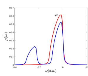
Figure 1: The hole spectral functions of the model interacting electron gas (blue) and the non-interacting electron gas (red), labelled $\rho_{0}$. The Fermi level is at the zero of the energy, indicated by a vertical line. The peak at around $\omega=-0.25$ is the plasmon satellite, located at one plasmon energy below the main quasiparticle peak. The model corresponds to $r_{s}=4$, giving a plasmon frequency $\omega_{\mathrm{p}}=0.217$. A quasiparticle renormalization factor $Z=0.7$, a band-narrowing $\alpha=0.8$, and a broadening $\eta=0.005$ have been used.

II.2.1 The exchange-correlation field and the kinetic potential

Consider the case $t<0$. Defining

$$I_{n} =\int_{0}^{k_{\mathrm{F}}}dkk^{2n}e^{-i\alpha k^{2}t/2}.$$ (46)

one obtains

$$\frac{1}{\Omega}\sum_{k\leq k_{\mathrm{F}}}A_{1} =\frac{1}{2\pi^{2}}Z\frac{\alpha-1}{2}I_{2},$$ (47)

$$\frac{1}{\Omega}\sum_{k\leq k_{\mathrm{F}}}A_{2} =\frac{1}{2\pi^{2}}(1-Z)e^{i\omega_{\mathrm{p}}t}\left(\frac{\alpha-1}{2}I_{2}-\omega_{\mathrm{p}}I_{1}\right),$$ (48)

$$\frac{1}{\Omega}\sum_{k\leq k_{\mathrm{F}}}(C_{1}+C_{2}) =\frac{1}{2\pi^{2}}\left[Z+(1-Z)e^{i\omega_{\mathrm{p}}t}\right]I_{1}.$$ (49)

Using the above results leads to

$$\left[i\partial_{t}-h(R)\right]G(R,t<0)|_{R=0}=\frac{i}{2\pi^{2}}[a_{2}I_{2}-a_{1}I_{1}],$$ (50)

$$G(0,t<0)=\frac{i}{2\pi^{2}}c_{1}I_{1}$$ (51)

where

$$a_{1} =\omega_{\mathrm{p}}(1-Z)e^{i\omega_{\mathrm{p}}t}$$ (52)

$$c_{1} =Z+(1-Z)e^{i\omega_{\mathrm{p}}t}.$$ (53)

$$a_{2} =\frac{\alpha-1}{2}c_{1}$$ (54)

The exchange-correlation field becomes

$$V_{\mathrm{xc}}(t<0)=\frac{1}{2}(\alpha-1)\frac{I_{2}}{I_{1}}-\frac{a_{1}}{c_{1}}.$$ (56)

To calculate the difference in the kinetic potentials one needs

$$-i\nabla\cdot\mathbf{j} =\frac{1}{\Omega}\sum_{k\leq k_{\mathrm{F}}}\frac{k^{2}}{2}(C_{1}+C_{2})=\frac{1}{4\pi^{2}}c_{1}I_{2}$$ (57)

$$-i\nabla\cdot\mathbf{j}^{\mathrm{KS}} =\frac{1}{\Omega}\sum_{k\leq k_{\mathrm{F}}}\frac{k^{2}}{2}e^{-itk^{2}/2}=\frac{1}{4\pi^{2}}I^{0}_{2},$$ (58)

where

$$I^{0}_{n} =\int_{0}^{k_{\mathrm{F}}}dkk^{2n}e^{-ik^{2}t/2}.$$ (59)

The temporal densities are given by

$$\rho_{0}(t<0)=-iG_{0}(0,t<0)=\frac{1}{2\pi^{2}}I^{0}_{1},$$ (60)

$$\rho(t<0)=-iG(0,t<0)=\frac{1}{2\pi^{2}}c_{1}I_{1},$$ (61)

yielding

$$V_{\mathrm{K}}(t<0) =\frac{1}{2}\frac{I_{2}}{I_{1}},$$ (62)

$$V^{\mathrm{KS}}_{\mathrm{K}}(t<0) =\frac{1}{2}\frac{I^{0}_{2}}{I^{0}_{1}}.$$ (63)

It is interesting to note that the kinetic potential does not depend on the plasmon energy and it cancels a term proportional to $I_{2}/I_{1}$ in the exchange-correlation field:

$$V_{\mathrm{xc}}+V_{\mathrm{K}} =\frac{\alpha}{2}\frac{I_{2}}{I_{1}}-\frac{a_{1}}{c_{1}}.$$ (64)

Using the relation

$$\frac{\partial I_{1}}{\partial t}=-\frac{i\alpha}{2}I_{2},$$ (65)

the exchange-correlation field and the kinetic potential can be rewritten as

$$V_{\mathrm{xc}}(t<0)=\frac{\alpha-1}{\alpha}i\partial_{t}\ln{I_{1}}-\frac{a_{1}}{c_{1}},$$ (66)

and

$$V_{\mathrm{K}} =\frac{i}{\alpha}\partial_{t}\ln{I_{1}},$$ (67)

so that

$$V_{\mathrm{xc}}+V_{\mathrm{K}} =i\partial_{t}\ln{I_{1}}-\frac{a_{1}}{c_{1}}.$$ (68)

The kinetic potential cancels a term in $V_{\mathrm{xc}}$ to give the correct band narrowing.

The first term of $V_{\mathrm{xc}}+V_{\mathrm{K}}$ when integrated over time from $0$ to $t$ is given by

$$-i\int_{0}^{t}dt^{\prime}i\frac{\partial}{\partial t^{\prime}}\ln{I_{1}} =\ln{\frac{I_{1}(t)}{I_{1}(0)}}$$ (69)

and the second is given by

$$i\int_{0}^{t}dt^{\prime}\frac{a_{1}}{c_{1}} =i\omega_{\mathrm{p}}\int_{0}^{t}dt^{\prime}\frac{(1-Z)e^{i\omega_{\mathrm{p}}t^{\prime}}}{Z+(1-Z)e^{i\omega_{\mathrm{p}}t^{\prime}}}$$

$$=\ln{\left[Z+(1-Z)e^{i\omega_{\mathrm{p}}t}\right]}.$$ (70)

Collecting the above two terms leads to

$$e^{-i\int_{0}^{t}dt^{\prime}[V_{\mathrm{xc}}(t^{\prime})+V_{\mathrm{K}}(t^{\prime})]}=\left[Z+(1-Z)e^{i\omega_{\mathrm{p}}t}\right]\frac{I_{1}(t)}{I_{1}(0)}.$$ (71)

Since $I_{1}(0)=2\pi^{2}\rho(r)$, the formal solution in Eq. (16) is then

$$\rho(r,t)=\frac{1}{2\pi^{2}}[Z+(1-Z)e^{i\omega_{\mathrm{p}}t}]I_{1}(t),$$ (72)

which reproduces the temporal density in Eq. (61).

II.3 Results

Atomic units are used throughout. A quasiparticle renormalization factor $Z=0.7$, a band-narrowing parameter $\alpha=0.8$, and a broadening $\eta=0.005$ have been used for all values of $r_{s}$.

In Fig. 1, the hole spectral function of the model for $r_{s}=4$ is compared with that of the non-interacting electron gas. The model essentially accounts for the quasiparticle band narrowing and the transfer of the quasiparticle weight to the plasmon satellite, located at one plasmon energy below the quasiparticle band. For simplicity, only one plasmon is taken into account and there is no weight arising from states above the Fermi level. The Fermi level of the interacting model has been adjusted to coincide with that of the non-interacting one.

From the model Green function, the exchange-correlation fields can be extracted as detailed in the theory section. The results are shown in Figs. 2 and 3 for the real and imaginary parts of $V_{\mathrm{xc}}$ and $\tilde{V}_{\mathrm{xc}}$. The former exhibits a more distinct periodicity whereas the latter appears to have a less well-defined periodicity. This can be understood from Fig. 5, which shows the difference between $\tilde{V}_{\mathrm{xc}}$ and $V_{\mathrm{xc}}$. This difference, which is also the difference in kinetic potential between the interacting system and the non-interacting Kohn-Sham system, has a beat pattern which decreases in magnitude as $-t$ increases. The price of approximating the interacting kinetic potential by that of the Kohn-Sham system and transferring the difference into the exchange-correlation field is a more irregular behavior of the latter.

In Fig. 4 the kinetic potentials of the interacting system and the non-interacting Kohn-Sham system are shown, both displaying well-defined oscillations. The interacting kinetic potential mimics the behavior of the Kohn-Sham kinetic potential but with a shifted phase, which appears to be time dependent. This suggests that rather than approximating the interacting kinetic potential by that of the Kohn-Sham system and shifting the difference into the exchange-correlation field, it could be more favorable to model directly the interacting kinetic potential by the Kohn-Sham one but with a time-dependent shifted phase. The phase shift between the two kinetic potentials increases as the density is lowered, indicating that at high density the Kohn-Sham kinetic potential better approximates the interacting kinetic potential. This is as anticipated as correlations are expected to be less important as the density increases.

There is a general trend of the exchange-correlation field and the kinetic potential as functions of $r_{s}$. The smaller $r_{s}$ or the higher the density the more oscillatory the quantities become. This is understandable since the oscillatory behavior of the exchange-correlation field is determined to a large extent by the plasmon energy, which increases with the density. The kinetic potential, on the other hand, does not follow the same oscillatory behavior of the exchange-correlation field since it does not depend explicitly on the plasmon energy, as can be seen in Eq. (63). In the case of the kinetic potential, it is the Fermi wavevector that determines the oscillatory behavior, which increases as the density increases or as $r_{s}$ decreases.

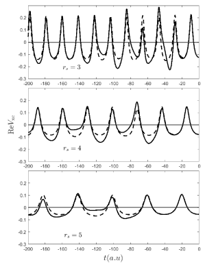
Figure 2: The real part of the exchange-correlation potentials $V_{\mathrm{xc}}$ (dashed) and $\tilde{V}_{\mathrm{xc}}$ (solid) as defined in the text for $r_{s}=3,4,5$. The difference, $\Delta V_{\mathrm{K}}=\tilde{V}_{\mathrm{xc}}-V_{\mathrm{xc}}$, is shown in Fig. 5.

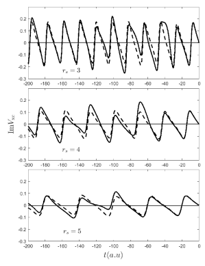
Figure 3: The imaginary part of the exchange-correlation potentials $V_{\mathrm{xc}}$ (dashed) and $\tilde{V}_{\mathrm{xc}}$ (solid) as defined in the text for $r_{s}=3,4,5$. The difference, $\Delta V_{\mathrm{K}}=\tilde{V}_{\mathrm{xc}}-V_{\mathrm{xc}}$, is shown in Fig. 5.

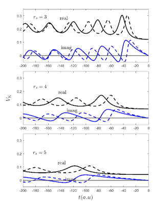
Figure 4: The real (black) and imaginary (blue) parts of the kinetic potentials $V_{\mathrm{K}}$ (solid) and $V^{\mathrm{KS}}_{\mathrm{K}}$ (dashed) as defined in the text for $r_{s}=3,4,5$.

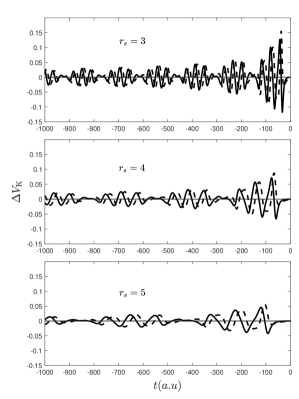
Figure 5: The real part (solid) and the imaginary part (dashed) of the kinetic potential difference $\Delta V_{\mathrm{K}}=V_{\mathrm{K}}-V^{\mathrm{KS}}_{\mathrm{K}}$ for $r_{s}=3,4,5$.

III Summary and conclusions

The continuity equation for the temporal density has been derived, starting from the recently proposed dynamical exchange-correlation field framework. The current density, which is an unknown quantity in this equation, is approximated by that of the Kohn-Sham system and the difference is transferred into the exchange-correlation field. There remains the task of finding a good approximation for the exchange-correlation field, which should be substantially simplified since only the diagonal part is needed. If a good approximation for the exchange-correlation field can be constructed, the spectral function can be readily calculated from an explicit solution to the continuity equation. A model Green function of the interacting electron gas is used to illustrate the key quantities in the proposed formulation.

References

(1) M. Gatti, V. Olevano, L. Reining, and I. V. Tokatly,
Phys. Rev. Lett. 99, 057401 (2007).
(2) S. Y. Savrasov and G. Kotliar,
Phys. Rev. B 69, 245101 (2004).
(3)F. Aryasetiawan, Phys. Rev. B 105, 075106 (2022).
(4)F. Aryasetiawan and T. Sjöstrand,
Phys. Rev. B 106, 045123 (2022).
(5)W. Kohn and L. J. Sham, Phys. Rev. 140, A1133 (1965).
(6)R. O. Jones and O. Gunnarsson, Rev. Mod. Phys.
61, 689 (1989).
(7)A. D. Becke, J. Chem. Phys. 140, 18A301 (2014).
(8)
R. O. Jones, Rev. Mod. Phys. 87, 897 (2015).
(9)L. Hedin, Phys. Rev. 139, A796 (1965).
(10)L. Hedin and S. Lundqvist, Solid State Physics 23, eds.
F. Seits, D. Turnbull, and H. Ehrenreich, Academic Press, NY, (1969).
(11)F. Aryasetiawan and O. Gunnarsson, Rep. Prog. Phys.
61, 237 (1998).
(12) D. C. Langreth, Phys. Rev. B 1, 471 (1970).
(13)B. Bergersen, Can. J. Phys. 51, 102 (1973).
(14)L. Hedin, Phys. Scr. 21, 477 (1980).
(15) C.-O. Almbladh and L. Hedin,
in Handbook on Synchroton Radiation,
edited by E. E. Koch (North-Holland, Amsterdam, 1983) Vol. 1, p.686.
(16) F. Aryasetiawan, L. Hedin, and K. Karlsson,
Phys. Rev. Lett. 77, 2268 (1996).
(17) J. J. Kas, J. J. Rehr, and L. Reining,
Phys. Rev. B 90, 085112 (2014).
(18) K. Karlsson and F. Aryasetiawan,
arXiv:2301.05590v1 [cond-matt.str-el] (2023).