Strain-tuned quantum criticality in electronic Potts-nematic systems

Abstract

Motivated by recent observations of threefold rotational symmetry breaking in twisted moiré systems, cold-atom optical lattices, quantum Hall systems, and triangular antiferromagnets, we phenomenologically investigate the strain-temperature phase diagram of the electronic 3-state Potts-nematic order. While in the absence of strain the quantum Potts-nematic transition is first-order, quantum critical points (QCP) emerge when uniaxial strain is applied, whose nature depends on whether the strain is compressive or tensile. In one case, the nematic amplitude jumps between two non-zero values while the nematic director remains pinned, leading to a symmetry-preserving meta-nematic transition that terminates at a quantum critical end-point. For the other type of strain, the nematic director unlocks from the strain direction and spontaneously breaks an in-plane twofold rotational symmetry, which in twisted moiré superlattices triggers an electric polarization. Such a piezoelectric transition changes from first to second-order upon increasing strain, resulting in a quantum tricritical point. Using a Hertz-Millis approach, we show that these QCPs share interesting similarities with the widely studied Ising-nematic QCP. The existence of three minima in the nematic action also leaves fingerprints in the strain-nematic hysteresis curves, which display multiple loops. At non-zero temperatures, because the upper critical dimension of the 3-state Potts model is smaller than three, the Potts-nematic transition is expected to remain first-order in 3D, but to change to second-order in 2D. As a result, the 2D strain-temperature phase diagram displays two first-order transition wings bounded by lines of critical end-points or tricritical points, reminiscent of the phase diagram of metallic ferromagnets. We discuss how our results can be used to unambiguously identify spontaneous Potts-nematic order.

I Introduction

Electronic nematicity, which consists of the electronically-driven breaking of the discrete rotational symmetry of a system (Kivelson et al., 1998), has been observed in various correlated electronic materials, including three families of unconventional superconductors: cuprates (Kivelson et al., 2003; Hinkov et al., 2008; Vojta, 2009), heavy-fermion compounds (Okazaki et al., 2011; Ronning et al., 2017; Seo et al., 2020), and iron-based materials (Chu et al., 2012; Fernandes et al., 2014; Böhmer and Meingast, 2016; Böhmer et al., 2022). In all those cases, the underlying tetragonal lattice renders the electronic nematic order parameter Ising-like (Fradkin et al., 2010), as the system must select between two nearest-neighbor (or next-nearest-neighbor) bonds of the square lattice, which are related by a $90^{\circ}$ rotation. The selected bond will either expand or contract, since nematic order necessarily triggers a lattice distortion (Fernandes et al., 2014). Conversely, application of uniaxial strain along one of the bond directions completely lifts the degeneracy between the two bonds, leading to a smearing of the nematic phase transition. The situation is analogous to the case of an Ising ferromagnet in the presence of a longitudinal magnetic field, since strain acts as a conjugate field to the nematic order parameter. Due to the ubiquituous presence of residual and random strain in crystals (Carlson et al., 2006; Carlson and Dahmen, 2011; Meese et al., 2022), this property can make it experimentally challenging to distinguish whether an anisotropic property is due to spontaneous nematic order, nematic order induced by strain (perhaps associated with an enhanced nematic susceptibility), or simply strain (Wang et al., 2022a). More broadly, the intrinsic coupling between electronic nematicity and uniaxial strain gives rise to a rich phenomenology (Karahasanovic and Schmalian, 2016; Paul and Garst, 2017; de Carvalho and Fernandes, 2019; Massat et al., 2022).

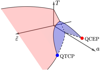
Figure 1: Qualitative $(\tilde{\varepsilon},a,T)$ phase diagram of a 2D Potts-nematic system, displaying first-order transition wings (blue surfaces). Here, $a$ is a non-thermal tuning parameter like doping or pressure; $\tilde{\varepsilon}$ is linearly proportional to the uniaxial strain applied along one of the high-symmetry directions of the threefold rotationally-symmetric lattice, but its sign depends on Landau coefficients of the Potts-nematic action. For $\tilde{\varepsilon}<0$, the isolated wing of first-order transitions is bounded by a line of classical end-points that terminates at a quantum critical end-point (QCEP). No symmetries are broken across this meta-nematic transition. For $\tilde{\varepsilon}>0$, the wing is bounded by a line of classical tricritical points terminating at a quantum tricritical point (QTCP), and is thus surrounded by a surface of continuous transitions (red surface). The in-plane two-fold rotational symmetry is broken spontaneously across these transitions, giving rise to a piezoelectric phase in twisted moiré systems.

Recently, electronic nematic order has also been observed in systems whose underlying lattices have threefold rotational symmetry (i.e. triangular, honeycomb, and kagome), such as the hexagonal (111) surface of bismuth subjected to large magnetic fields (Feldman et al., 2016), the trigonal lattice of the doped topological insulator Bi₂Se₃ (Sun et al., 2019; Cho et al., 2020), the triangular antiferromagnet Fe_1/3NbS₂ (Little et al., 2020), a triangular optical lattice of cold ⁸⁷Rb atoms (Jin et al., 2021a), and the trangular moiré superlattices of twisted bilayer graphene (TBG) (Kerelsky et al., 2019; Jiang et al., 2019; Choi et al., 2019; Cao et al., 2021), twisted double-bilayer graphene (TDBG) (Rubio-Verdú et al., 2022), twisted trilayer graphene (Zhang et al., 2022), and heterobilayer transition metal dichalcogenides (Jin et al., 2021b). More broadly, Potts-nematicity has been proposed to emerge in diverse settings, from frustrated magnets (Mulder et al., 2010; Drouin-Touchette et al., 2022; Li and Li, 2022; Nedić et al., 2022; Strockoz et al., 2022) to interacting moiré systems (Dodaro et al., 2018; Venderbos and Fernandes, 2018; Kozii et al., 2019; Xu et al., 2020; Fernandes and Venderbos, 2020; Kang and Vafek, 2020; Xie et al., 2021; Chichinadze et al., 2020; Sboychakov et al., 2020; Wang et al., 2021; Onari and Kontani, 2022; Brillaux et al., 2022; Matty and Kim, 2022) and kagome metals (Grandi et al., 2023). In contrast to the case of lattices with fourfold rotational symmetry, the nematic order parameter here has a 3-state Potts character (Hecker and Schmalian, 2018; Fernandes et al., 2019), corresponding to selecting one among three nearest-neighbor bonds related by a $120^{\circ}$ (or $60^{\circ}$) rotation. The linear coupling between such a Potts-nematic order parameter and in-plane strain has been recently explored in different contexts (Hecker and Schmalian, 2018; How and Yip, 2019; Kuntsevich et al., 2019; Fernandes and Venderbos, 2020; Kostylev et al., 2020; Little et al., 2020; Cao et al., 2021; Kimura et al., 2022; Hecker and Fernandes, 2022). An interesting result is that application of uniaxial strain along one of the bond directions may not fully lift the degeneracy between the three bonds. Consequently, unlike the case of a tetragonal lattice, a nematic-related transition – dubbed nematic-flop transition in Ref. (Fernandes and Venderbos, 2020)– can take place in a triangular lattice even in the presence of uniaxial strain. The situation is analogous to a 3-state Potts ferromagnet in the presence of an external magnetic field that points along one of the three allowed magnetic moment directions (Straley and Fisher, 1973; Blankschtein and Aharony, 1980). If a “positive” field is applied, i.e. a field that favors one of the moment directions, no additional symmetries can be spontaneously broken. However, if a “negative” field is applied, i.e. a field that penalizes one of the moment directions, there is a residual Ising symmetry associated with the two remaining moment directions. Such a symmetry is spontaneously broken in the vicinity of the zero-field ferromagnetic transition.

Another peculiarity of the 3-state Potts model is that its upper critical dimension is $d_{u}^{\mathrm{Potts}}\lesssim 3$ (for a review, see Ref. (Wu, 1982)), whereas in the Ising model, $d_{u}^{\mathrm{Ising}}=4$. Most importantly, the character of the 3-state Potts transition is fundamentally different for dimensions above and below $d_{u}^{\mathrm{Potts}}$. For $d\geq 3$, a mean-field description works and the transition is first-order, due to the existence of a cubic invariant in the Landau free-energy expansion. However, for $d=2$, the 3-state Potts transition is second-order. This has important consequences for two-dimensional systems subjected to a 3-state Potts nematic instability, such as twisted moiré systems. At high enough temperatures, $d=2$ and one expects a second-order nematic transition. However, at $T=0$, since $d+z>d_{u}^{\mathrm{Potts}}$ for the expected values of the dynamic critical exponent $z$ (i.e. $z=1$ for an insulator and $z=3$ for a metal (Löhneysen et al., 2007)), the nematic transition should be first-order. This not only implies the absence of a Potts-nematic quantum critical point (QCP), but it also indicates that, as the nematic transition temperature is suppressed by a non-thermal tuning parameter, a tricritical point should emerge.

In this paper, we use a phenomenological model to study the Potts-nematic phase diagram in the presence of uniaxial strain. The nematic order parameter is parametrized as a two-component “vector” $\boldsymbol{\Phi}=\phi\left(\cos 2\theta,\,\sin 2\theta\right)$, where $\phi$ is the magnitude and the director angle $\theta$ is restricted to $3$ possible values. The tuning parameters are the temperature $T$ and a non-thermal control parameter $a$, such as doping, which suppresses the Potts-nematic transition temperature to zero. Fig. 1 summarizes our main findings for a 2D system whose underlying lattice has threefold rotational symmetry. At $T=0$, since the system is above the 3-state-Potts upper critical dimension, it undergoes a first-order quantum nematic phase transition upon changing the non-thermal parameter $a$, where the threefold rotational symmetry $C_{3z}$ is broken. The fate of the transition upon application of uniaxial strain along one of the nematic-bond directions depends on the sign of $\tilde{\varepsilon}$, which is linearly proportional to the strain $\varepsilon$, which in turn can be either compressive ($\varepsilon<0$) or tensile ($\varepsilon>0$).

For $\tilde{\varepsilon}<0$, upon increasing the strain magnitude, a first-order transition line transition extends to larger $a$ values, ending at a quantum critical end-point (QCEP), analogously to the case of the liquid-gas transition of water. The magnitude of the nematic order parameter $\phi$ jumps across the first-order transition line, whereas the nematic director angle $\theta$ remains pinned by the strain direction, signaling a symmetry-preserving quantum meta-nematic transition. Beyond the QCEP, there is only a crossover signaled by the Widom line.

For $\tilde{\varepsilon}>0$, while a first-order transition line extending to larger values of $a$ also appears upon increasing the strain magnitude, the situation is completely different. The first key difference is that the director angle $\theta$ spontaneously unpins from the strain direction across the transition, selecting one among two possible angles, which in turn are related by twofold rotations with respect to in-plane axes (denoted by $C^{\prime}_{2}$). Therefore, across this first-order Ising transition, the $C^{\prime}_{2}$ symmetry is broken, resulting in the emergence of an out-of-plane ferroelectric polarization in the case of twisted moiré systems. Because this ferroelectricity only appears in the presence of strain of a particular type (compressive or tensile), we dub this a quantum piezoelectric transition. The second key difference with respect to the case of $\tilde{\varepsilon}<0$ is that, upon applying stronger strain, the first-order transition line ends at a quantum tricritical point (QTCP), beyond which a line of piezoelectric QCPs emerges. A Hertz-Millis type of calculation for both the piezoelectric QCPs and the meta-nematic QCEP in the case of metallic systems reveals that they behave very similarly to an Ising-nematic QCP (Oganesyan et al., 2001; Metzner et al., 2003; Garst and Chubukov, 2010; Metlitski and Sachdev, 2010; Schattner et al., 2016; Lederer et al., 2017; Klein and Chubukov, 2018), not only possessing the same dynamical critical exponent $z=3$, but also cold spots at the Fermi surface.

We also compute the upper and lower spinodal lines associated with the different first-order transition lines and employ a generalized Stoner-Wohlfarth approach (Stoner and Wohlfarth, 1948) to show that the asymmetry between the effects of compressive and tensile strains is manifested in the hysteresis curves of $\boldsymbol{\Phi}\left(\varepsilon\right)$. In particular, because there are three action minima available, rather than the usual two, the hysteresis curves can show multiple loops depending on the initial conditions. These characteristic features of the hysteresis curves provide concrete criteria to unambigously determine experimentally whether a twofold anisotropic signal observed in a system with threefold rotational symmetry is due to spontaneous nematic order or induced nematic order by strain.

The extension of the results to non-zero temperatures depends on the dimensionality of the system. For $d=3$, the system is always above the 3-state-Potts upper critical dimension, implying that the phase diagram at non-zero temperatures should be similar to that at $T=0$. However, for $d=2$, the Potts-nematic transition should generally become second-order at high enough temperatures, thus displaying the typical critical exponents of the 2D 3-state Potts model (Wu, 1982). Consequently, a tricritical point at $T\neq 0$ should exist for unstrained systems, connecting the first-order quantum phase transition to the second-order transition at high $T$. As illustrated in Fig. 1, this tricritical point is expected to directly connect to the QCEP and the QCTP, giving rise to two first-order transition wings. This shape of the phase diagram resembles that of an itinerant ferromagnet (Belitz et al., 2005; Brando et al., 2016), although the mechanisms by which the $T=0$ transition becomes first-order are unrelated (Belitz et al., 1999; Chubukov et al., 2004; Maslov and Chubukov, 2009). An important difference is that, in the Potts-nematic case, the first-order transition wing on the $\tilde{\varepsilon}<0$ side is isolated, bounded by the line of critical endpoints, whereas the wing on the $\tilde{\varepsilon}>0$ side is bounded by a line of tricritical points, and thus exists inside a much broader wing signaling the second-order transition to the piezoelectric phase.

The paper is organized as follows: in Sec. II we apply mean-field theory to determine the $T=0$ phase diagram of the Potts-nematic model, focusing on the emergence of the meta-nematic QCEP and the piezoelectric QTCP in Sec. II.2 and Sec. II.3, respectively. The Potts-nematic hysteresis curves are analyzed in Sec. III, whereas Sec. IV presents a qualitative analysis of the $T>0$ phase diagram. Conclusions are presented in Sec. V.

II Zero-temperature phase diagram

II.1 Mean-field solution of the Potts-nematic model

The “in-plane” nematic order parameter can always be parametrized as $\boldsymbol{\Phi}\equiv\left(\phi_{1},\,\phi_{2}\right)=\phi\left(\cos 2\theta,\,\sin 2\theta\right)$, where $\phi>0$ is the magnitude and $0\leq\theta\leq\pi$ is the nematic director angle (Fradkin et al., 2010; Fernandes and Venderbos, 2020). By construction, the order parameter satisfies $\boldsymbol{\Phi}(\theta)=\boldsymbol{\Phi}(\theta+\pi)$, as is the case for the classical nematic order parameter. Physically, the components $\phi\cos 2\theta$ and $\phi\sin 2\theta$ transform as the expectation values of the electronic quadrupolar moments $\rho_{x^{2}-y^{2}}$ and $\rho_{xy}$, as well as the strain components $\varepsilon_{xx}-\varepsilon_{xy}$ and $\varepsilon_{xy}$. Here, $\varepsilon_{ij}=\left(\partial_{i}u_{j}+\partial_{j}u_{i}\right)/2$ is the strain tensor and $\boldsymbol{u}$, the displacement vector. The allowed values of $\theta$ are constrained by the symmetries of underlying crystal lattice, as well as by the presense of in-plane uniaxial strain. Hereafter, we focus on lattices that are invariant under threefold rotations with respect to the $z$ axis ($C_{3z}$ operation) and twofold rotations with respect to at least one in-plane axis ($C^{\prime}_{2}$ operation). These include the triangular lattice as well as any other lattice with point groups $\mathrm{D}_{\mathrm{6h}}$, $\mathrm{D}_{\mathrm{3h}}$, $\mathrm{D_{3d}}$, $\mathrm{D}_{\mathrm{6}}$, and $\mathrm{D_{3}}$. Note that the latter two describe certain twisted moiré superlattices, like TBG and TDBG. We assume that external uniaxial strain is applied along a direction that makes an angle $\alpha$ with respect to the $x$ axis, and consider both tensile ($\varepsilon>0$) and compressive ($\varepsilon<0$) strain. In this case, the nematic action is given by (Hecker and Schmalian, 2018; Fernandes and Venderbos, 2020; Xu et al., 2020; Cao et al., 2021):

$$\mathcal{S}_{\text{nem}}\left[\boldsymbol{\Phi}\left(q\right)\right]=\frac{1}{2}\int_{q}\phi_{-q}\chi_{0}^{-1}\left(q\right)\phi_{q}\\ +\int_{x}\left[\frac{\lambda}{3}\,\phi^{3}\cos 6\theta+\frac{u}{4}\,\phi^{4}-\gamma\varepsilon\phi\cos\left(2\theta-2\alpha\right)\right]$$ (1)

Here, $x=(\tau,\mathbf{x})$ denotes imaginary time $\tau\in[0,\beta]$ and spatial variable $\mathbf{x}$, whereas $q=(\Omega_{n},\boldsymbol{q})$ consists of bosonic Matsubara frequencies $\Omega_{n}=2\pi nT$ and momentum $\mathbf{q}$. The inverse nematic susceptibility is given by $\chi_{0}^{-1}(q)=a+\boldsymbol{q}^{2}+\Omega_{n}^{2}$, where $a$ is a non-thermal tuning parameter. The coupling constants $\lambda$ and $u>0$ describe the non-harmonic terms of the action, whereas $\gamma$ is the elasto-nematic coupling.

For $\varepsilon=0$, the action (1) maps onto the 3-state Potts model – or, equivalently, the $3$-state clock model. Indeed, for $\lambda>0$, the nematic director is pinned to the three high-symmetry directions $\theta=(2n+1)\pi/6$, whereas for $\lambda<0$, the three allowed values are $\theta=2n\pi/6$, with $n=0,1,2$. In the presence of strain, there are important changes in the problem. In this paper, we consider strain applied along one of the high-symmetry directions of the lattice. In this case, we can set without loss of generality $\alpha=2m\pi/6$, with $m=0,1,2$, since the action (1) is invariant under $\varepsilon\rightarrow-\varepsilon$ and $\alpha\rightarrow\alpha+\pi/2$. This invariance reflects the fact that, for the nematic order parameter, compressive strain applied along one axis has the same effect as tensile strain applied along an orthogonal axis. Shifting the director angle such that it is measured with respect to the strain direction, $\tilde{\theta}=\theta-\alpha$, and considering the case of static and homogeneous fields, the action “density” becomes:

$$S_{\text{nem}}\left(\boldsymbol{\Phi}\right)=\frac{a}{2}\,\phi^{2}+\frac{u}{4}\,\phi^{4}+\frac{\lambda}{3}\,\phi^{3}\cos 6\tilde{\theta}-\gamma\varepsilon\phi\cos 2\tilde{\theta}$$ (2)

Upon defining the rescaled quantities $\tilde{\phi}\equiv\frac{u}{\left|\lambda\right|}\,\phi$, $\tilde{S}_{\text{nem}}\equiv\frac{u^{3}}{\lambda^{4}}\,S_{\text{nem}}$, $\tilde{a}=\frac{u}{\lambda^{2}}\,a$, and $\tilde{\varepsilon}\equiv\frac{\gamma u^{2}}{\lambda^{3}}\,\varepsilon$, we can rewrite the action in a more convenient form:

$$\tilde{S}_{\text{nem}}=\frac{\tilde{a}}{2}\,\tilde{\phi}^{2}+\frac{1}{4}\,\tilde{\phi}^{4}+\mathrm{sgn}\lambda\left(\frac{1}{3}\,\tilde{\phi}^{3}\cos 6\tilde{\theta}-\tilde{\varepsilon}\tilde{\phi}\cos 2\tilde{\theta}\right)$$ (3)

Regardless of whether the system is 2D or 3D, at $T=0$ the effective dimensionality $d+z\geq 3$, implying that the system is above the upper critical dimension of the 3-state Potts model. As a result, a mean-field solution is appropriate; setting $\partial\tilde{S}_{\text{nem}}/\partial\tilde{\phi}=0$ and $\partial\tilde{S}_{\text{nem}}/\partial\tilde{\theta}=0$, and assuming $\tilde{\phi}\neq 0$, we find the mean-field equations:

$$\tilde{a}\tilde{\phi}+\mathrm{sgn}\lambda\,\tilde{\phi}^{2}\cos 6\tilde{\theta}+\tilde{\phi}^{3} =\mathrm{sgn}\lambda\,\tilde{\varepsilon}\cos 2\tilde{\theta}$$ (4)

$$\sin 6\tilde{\theta} =\frac{\tilde{\varepsilon}}{\tilde{\phi}^{2}}\sin 2\tilde{\theta}$$ (5)

To make the notation less cumbersome, hereafter we drop the tilde of all quantities except for $\tilde{\varepsilon}$; the latter is to emphasize that the relevant quantity is the combination $\tilde{\varepsilon}=\left(\gamma u^{2}/\lambda^{3}\right)\varepsilon$, whose overall sign depends not only on whether the applied strain $\varepsilon$ is compressive or tensile, but also on the signs of the nemato-elastic coupling $\gamma$ and on the cubic Landau coefficient $\lambda$. We first review the well-known results in the case of no applied strain, $\tilde{\varepsilon}=0$ (Hecker and Schmalian, 2018; Fernandes and Venderbos, 2020). Eq. (5) gives the extrema $\theta_{0}=p\pi/6$, with $p=0,\cdots,5$. Computing the second derivative of the action at the extrema, we find $\left(\frac{\partial^{2}S_{\text{nem}}}{\partial\theta^{2}}\right)_{\theta_{0}}=-12\phi^{3}(-1)^{p}\mathrm{sgn}\lambda$. Therefore, the minima (maxima) of the action are given by $\theta_{0}=p\pi/6$ with even (odd) $p$ if $\lambda<0$ and odd (even) $p$ if $\lambda>0$. Meanwhile, Eq. (4) becomes:

$$a-\phi_{0}+\phi_{0}^{2}=0$$ (6)

which gives:

$$\phi_{0,\pm}=\frac{1}{2}\left(1\pm\sqrt{1-4a}\right)$$ (7)

Clearly, a $\phi_{0}\neq 0$ solution can only exist if $a<a_{\mathrm{us}}\equiv 1/4$, which sets the upper spinodal of the first-order Potts-nematic transition. The first-order transition takes place for $a\equiv a_{c,0}$ such that $S_{\text{nem}}\left(\phi_{0,+},\theta_{0}\right)=0$, which gives $a_{c,0}=2/9$. The jump in the nematic order parameter at the transition is thus given by $\Delta\phi_{0}=1/3$.

The mean-field solution for non-zero strain has been in part discussed in Refs. (Fernandes et al., 2019; Cao et al., 2021) and, more broadly, in the literature of the 3-state Potts model under the presence of a magnetic field (Straley and Fisher, 1973; Blankschtein and Aharony, 1980; Wu, 1982). The second mean-field equation (5) can be rewritten as (where, we recall, the director angle $\theta$ is measured with respect to the direction strain is applied):

$$\sin 2\theta\left[\cos^{2}2\theta-\frac{1}{4}\left(1+\frac{\tilde{\varepsilon}}{\phi^{2}}\right)\right]=0$$ (8)

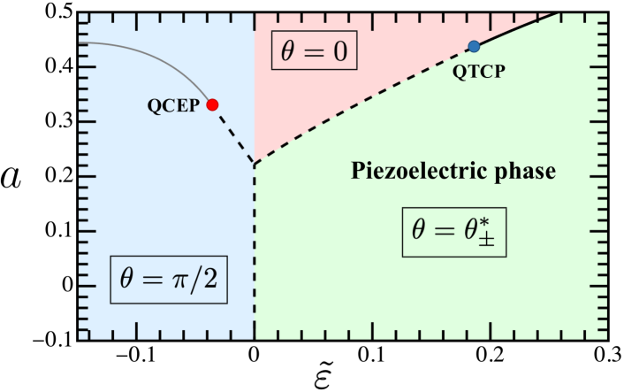
Figure 2: Zero-temperature $(\tilde{\varepsilon},a)$ phase diagram of a Potts-nematic system. The red and blue regions correspond to the phases in which the director angle $\theta$ is fixed to the high-symmetry directions $\theta_{+}=0$ and $\theta_{-}=\pi/2$, respectively, whereas the green region corresponds to the piezoelectric phase, in which $\theta=\theta_{\pm}^{*}$ is not fixed [see Eq. (12)]. For $\tilde{\varepsilon}<0$, there is a first-order meta-nematic transition line (dashed black) that ends at a QCEP. Beyond the QCEP, there is a crossover signaled by the Widom line (solid gray). For $\tilde{\varepsilon}>0$, the first-order piezoelectric transition, which spontaneously breaks in-plane two-fold rotational symmetry, ends at a QTCP, after which it becomes second-order (solid black line).

This equation always admits two solutions: $\theta_{+}=0$, corresponding to a nematic director parallel to the strain direction, and $\theta_{-}=\pi/2$, denoting a nematic director perpendicular to the strain direction. Note that, by definition, $\mathbf{\Phi}\rightarrow-\mathbf{\Phi}$ upon a rotation of $90^{\circ}$ of the director angle $\theta$. In both cases, the mean-field equation (4) that determines the $\phi_{\pm}$ values corresponding to $\theta_{\pm}$ is:

$$a\phi_{\pm}+\phi_{\pm}^{3}\pm\mathrm{sgn}\lambda\,\left(\phi_{\pm}^{2}-\tilde{\varepsilon}\right)=0$$ (9)

whereas the action evaluated at these extrema is given by:

$$S_{\pm}=\frac{a}{2}\,\phi_{\pm}^{2}+\frac{1}{4}\,\phi_{\pm}^{4}\pm\mathrm{sgn}\lambda\left(\frac{1}{3}\,\phi_{\pm}^{3}-\tilde{\varepsilon}\phi_{\pm}\right)$$ (10)

To check which of these solutions (if any) is a minimum of the action, we evaluate the second derivative:

$$\left(\frac{\partial^{2}S_{\mathrm{nem}}}{\partial\theta^{2}}\right)_{\theta_{\pm}}=\pm 4\mathrm{sgn}\lambda\,\phi_{\pm}\tilde{\varepsilon}\left(1-\frac{3\phi_{\pm}^{2}}{\tilde{\varepsilon}}\right)$$ (11)

It follows that, when $\tilde{\varepsilon}<0$, the $\theta_{-}$ ($\theta_{+}$) solution is always a local action minimum for $\lambda>0$ ($\lambda<0$). Meanwhile, when $\tilde{\varepsilon}>0$, the situation is more involved. Far enough from the Potts-nematic transition of the unstrained system, where the nematic order parameter induced by the strain is expected to be small, $\phi^{2}\ll\tilde{\varepsilon}$, we find that the $\theta_{+}$ ($\theta_{-}$) solution is a local minimum of the action for $\lambda>0$ ($\lambda<0$). Once the nematic order parameter increases such that $\phi^{2}>\tilde{\varepsilon}/3$, however, this solution switchs to a local maximum. This indicates that another solution is available. Indeed, the mean-field equation for $\theta$, Eq. (8), admits two additional solutions:

$$\theta_{\pm}^{*}=\pm\frac{1}{2}\arccos\left(\frac{1}{2}\sqrt{1+\frac{\tilde{\varepsilon}}{\phi^{2}}}\right)$$ (12)

provided that the argument is smaller than $1$, i.e. $\phi^{2}>\tilde{\varepsilon}/3$. This is the same condition for which the $\theta_{+}$ ($\theta_{-}$) solution becomes a local maximum of the action for $\lambda>0$ ($\lambda<0$). Note that, in the director space spanned by the angle $\theta$, the points $\theta_{+}^{*}$ and $\theta_{-}^{*}$ are related by a twofold rotation with respect to the horizontal axis (as well as the vertical axis), which indicates that selecting one of the two solutions will break a spatial symmetry of the system. We will return to this point later. Using Eq. (12), it is straightforward to obtain the mean-field equation for the corresponding nematic amplitude $\phi_{\pm}^{*}$

$$a\phi_{\pm}^{*}+\left(\phi_{\pm}^{*}\right)^{3}\mp\mathrm{sgn}\lambda\,\phi_{\pm}^{*}\sqrt{\tilde{\varepsilon}+\left(\phi_{\pm}^{*}\right)^{2}}=0$$ (13)

as well as the values of the action evaluated at these solutions:

$$S_{\pm}^{*}=\frac{a}{2}\left(\phi_{\pm}^{*}\right)^{2}+\frac{1}{4}\left(\phi_{\pm}^{*}\right)^{4}\mp\frac{\mathrm{sgn}\lambda}{3}\left[\tilde{\varepsilon}+\left(\phi_{\pm}^{*}\right)^{2}\right]^{3/2}$$ (14)

Eq. (13) can be solved in a straightforward way:

$$\phi_{\pm}^{*}=\sqrt{\frac{1}{2}-a\pm\sqrt{\tilde{\varepsilon}-a+\frac{1}{4}}}$$ (15)

It turns out that the $\phi_{-}^{*}$ solution is either a saddle-point of the action or does not satify the condition $\phi^{2}<\tilde{\varepsilon}/3$. Consequently, $\phi_{+}^{*}$ is the desired solution, yielding:

$$\theta_{\pm}^{*}=\pm\frac{1}{2}\arccos\left(\frac{1}{2}\left[1+\frac{\tilde{\varepsilon}}{\frac{1}{2}-a+\sqrt{\tilde{\varepsilon}-a+\frac{1}{4}}}\right]^{1/2}\right)$$ (16)

We therefore obtain three different viable solutions for $\tilde{\varepsilon}\neq 0$: $\theta_{+}=0$, $\theta_{-}=\pi/2$, and $\theta_{\pm}^{*}$ given by Eq. (16). Following our analysis above, either $\theta_{-}$ or $\theta_{+}$ is expected to be the global minimum for $\tilde{\varepsilon}<0$, depending on whether $\lambda>0$ or $\lambda<0$, respectively. On the other hand, for $\tilde{\varepsilon}>0$, two different minima are expected for distinct ranges of $a$: $\theta_{+}$ or $\theta_{-}$ (for $\lambda>0$ and $\lambda<0$, respectively) and $\theta_{\pm}^{*}$.

The full phase diagram can be directly obtained by comparing the actions evaluated at the three solutions, Eqs. (10) and (14), after solving for the corresponding nematic amplitude in Eqs. (9) and (16). The resulting phase diagram is shown in Fig. 2; as anticipated, it is analogous to the phase diagram of the ferromagnetic 3-state Potts-model in the presence of a magnetic field (Straley and Fisher, 1973; Blankschtein and Aharony, 1980). For concreteness, we consider the case in which $\lambda>0$. For $\tilde{\varepsilon}<0$, we indeed find that the $\theta_{-}=\pi/2$ solution is the global minimum for any value of $a$. This does not mean, however, that the system does not undergo a phase transition. As denoted by the dashed line in Fig. 2, for small enough $\left|\tilde{\varepsilon}\right|$ and close enough to the nematic transition at zero strain, $a_{c}=2/9$, the system undergoes a symmetry-preserving first-order transition in which the nematic amplitude $\phi_{-}$ jumps, while the nematic director angle $\theta$ remains fixed. This is expected, since the nematic order parameter undergoes a first-order transition in the absence of strain and $\tilde{\varepsilon}$ acts as a conjugate field to the nematic order parameter. We dub this a meta-nematic quantum phase transition, in analogy to the $T=0$ meta-magnetic transition that takes place in a metallic ferromaget subjected to an external field. The first-order line ends in a critical end-point, similarly to the liquid-gas transition of water. This side of the phase diagram is further discussed in Sec. II.2.

The $\tilde{\varepsilon}>0$ side of the phase diagram is qualitatively different. As displayed in Fig. 2, for $a\gg a_{c}$, the global minimum is at $\theta_{+}=0$. However, upon approaching the nematic transition point of the unstrained system, $a_{c,0}=2/9$, the nematic director angle that minimizes the action switches to $\theta_{\pm}^{*}$. In contrast to the transition on the $\tilde{\varepsilon}<0$ side of the phase diagram, this is not a symmetry-preserving transition, since the spatial symmetry that relates the two nematic director angles $\theta_{+}^{*}$ and $\theta_{-}^{*}$ is spontaneously broken. For small enough $\tilde{\varepsilon}$, this transition is first-order whereas for large enough $\tilde{\varepsilon}$, it becomes second-order. Therefore, there is a tricritical point, marked in the figure, for intermediate values of $\tilde{\varepsilon}$. We will analyze this side of the phase diagram in more detail in Sec. II.3.

The change in the nematic director angle upon decreasing $a$ for $\tilde{\varepsilon}>0$, discussed also in Ref. (Fernandes and Venderbos, 2020), can be understood directly from the action in Eq. (3). For $\lambda>0$, the cubic term is minimized for $\theta=\pi/6,\,\pi/2,\,5\pi/6$ and maximized for $\theta=0,\,\pi/3,\,2\pi/3$. The linear term, on the other hand, is minimized by $\theta=\pi/2$ and maximized by $\theta=0$, for $\tilde{\varepsilon}<0$, and minimized by $\theta=0$ and maximized by $\theta=\pi/2$ for $\tilde{\varepsilon}>0$. Therefore, in the regime $\tilde{\varepsilon}<0$, both the linear and cubic terms can be simultaneously minimized by the same nematic director angle, $\theta=\pi/2$. In contrast, in the regime $\tilde{\varepsilon}>0$, the minimum of the cubic term is the maximum of the linear term and vice versa. For large enough values of $a$, where the amplitude of the nematic order parameter is small, the linear term wins over the cubic one. Once the system approaches its intrinsic nematic instability, the nematic ampitude increases and the two terms eventually give comparable contributions to the action. This frustration between the minima and maxima of the cubic and linear terms is lifted by a compromise value for the nematic director $\theta$. Indeed, Eq. (12) for $\theta_{\pm}^{*}$ interpolates between $0$ when $\phi^{2}=\tilde{\varepsilon}/3$, which mimizes the linear term, to $\pi/6$ and $5\pi/6$ when $\phi^{2}\gg\tilde{\varepsilon}/3$, which mimizes the cubic term.

II.2 Meta-nematic quantum critical endpoint

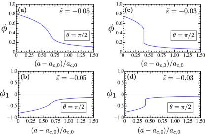
Figure 3: Behavior of the nematic order parameter for fixed $\tilde{\varepsilon}<0$ across the crossover Widom line [panels (a) and (b)] and the meta-nematic transition line [panels (c) and (d)], as defined in the phase diagram of Fig. 2. Representative values of $\tilde{\varepsilon}$ are chosen from the left and right side of $\tilde{\varepsilon}_{\text{QCEP}}=-1/27\approx-0.037$, respectively. The top panels show the magnitude of the nematic order parameter $\phi$ and the bottom panels, the nematic component projected along the strain direction, $\phi_{1}=\phi\cos 2\theta$; in all cases, the nematic director angle remains fixed at $\pi/2$. The horizontal axis corresponds to the non-thermal tuning parameter $a$ measured relative to unstrained Potts-nematic transition point $a_{c,0}=2/9$.

To gain further insight into the $\tilde{\varepsilon}<0$ region of the phase diagram, we substitute the value of the nematic director angle that minimizes the action, $\theta_{-}=\pi/2$, in Eq. (3) – recall that we are considering $\lambda>0$. We then obtain an action that depends only on the magnitude $\phi$:

$$S_{\text{nem}}^{(\tilde{\varepsilon}<0)}\left(\phi\right)=\frac{a}{2}\,\phi^{2}+\frac{1}{4}\,\phi^{4}-\frac{1}{3}\,\phi^{3}+\tilde{\varepsilon}\phi$$ (17)

To proceed, we recall that, for zero strain, $\tilde{\varepsilon}=0$, the system undergoes a first-order transition at $a_{c,0}=2/9$ in which the nematic order parameter jumps by $\Delta\phi_{0}=1/3$. Therefore, it is convenient to introduce the shifted nematic order parameter $\delta\phi\equiv\phi-\Delta\phi_{0}$, as it effectively removes the cubic term above. We find:

$$S_{\text{nem}}^{(\tilde{\varepsilon}<0)}\left(\delta\phi\right)=\frac{A}{2}(\delta\phi)^{2}+\frac{1}{4}(\delta\phi)^{4}-H\,\delta\phi$$ (18)

where we dropped a constant term and defined:

$$A \equiv a-\frac{1}{3}$$ (19)

$$H \equiv-\tilde{\varepsilon}-\frac{1}{3}\left(a-a_{c,0}\right)$$ (20)

Eq. (18) is nothing but the Ising model in the presence of an external field $H$, widely employed to describe symmetry-preserving phase transitions, such as the Mott transition (Terletska et al., 2011; Furukawa et al., 2015) and certain magnetic transitions (Wang et al., 2022b). It consists of a first-order transition line parametrized by $H=0$, below which the order parameter $\phi$ jumps between two non-zero values, signaling a meta-nematic transition. The first-order transition line – and thus the jump in $\phi$ – terminates at the so-called critical end-point, given by $A=H=0$, which in our case is a quantum critical end-point (QCEP), since the system is at $T=0$. This allows us to obtain the location of the QCEP in the $\left(\tilde{\varepsilon},a\right)$ phase diagram,

$$a_{\text{QCEP}} =\frac{1}{3}$$ (21)

$$\tilde{\varepsilon}_{\text{QCEP}} =-\frac{1}{27}$$ (22)

as well as the equation describing the first-order transition line:

$$a_{c}\left(\tilde{\varepsilon}\right)=\frac{2}{9}-3\tilde{\varepsilon}\,,\quad\mathrm{for}\;\,\tilde{\varepsilon}_{\text{QCEP}}<\tilde{\varepsilon}<0\,.$$ (23)

The behavior of the magnitude of the nematic order parameter, $\phi$, and of the nematic component projected along the strain direction, $\phi_{1}=\phi\cos 2\theta$, is shown in Fig. 3 as a function of the non-thermal tuning parameter $a$ for fixed values of strain $\tilde{\varepsilon}<0$. For $\tilde{\varepsilon}<\tilde{\varepsilon}_{\text{QCEP}}$, as shown in Figs. 3(a)-(b), the nematic order parameter evolves continuously and displays a crossover behavior at a characteristic $a$ value corresponding to the Widom line located at the left of the QCEP. On the other hand, for $\tilde{\varepsilon}>\tilde{\varepsilon}_{\text{QCEP}}$, the nematic order parameter undergoes a jump between two non-zero values, signaling a symmetry-preserving meta-nematic transition, as shown in Figs. 3(c)-(d).

To characterize the properties of the QCEP, we calculate, the dynamical critical exponent $z$. For an insulator, the bare dynamics of the nematic susceptibility $\chi_{0}\left(q\right)$ is unchanged by the coupling to the electrons, resulting in $z=1$. For a metal, we employ a Hertz-Millis approach (Hertz, 1976; Millis et al., 2002; Löhneysen et al., 2007) to compute the one-loop polarization bubble $\Pi\left(q\right)$ that renormalizes the nematic susceptibility, $\chi^{-1}\left(q\right)=\chi_{0}^{-1}\left(q\right)-\Pi\left(q\right)$. As discussed elsewhere (Xu et al., 2020; Fernandes and Venderbos, 2020), for a single-band system, the interaction (with coupling constant $g$) between the nematic field $\boldsymbol{\Phi}$ and the electronic quadrupolar charge density is given by the Hamiltonian:

$$H_{I}=g\phi\sum_{\mathbf{k}}\cos\left(2\beta_{\mathbf{k}}-2\theta\right)c_{\mathbf{k+q}/2,\sigma}^{\dagger}c_{\mathbf{k-q}/2,\sigma}^{\phantom{}}$$ (24)

where $\tan\beta_{\mathbf{k}}\equiv k_{y}/k_{x}$ and the annihilation operator $c_{\mathbf{k},\sigma}$ refers to an electron with momentum $\mathbf{k}$ and spin $\sigma$. Spin indices are implicitly summed. Recall that, in our notation, $\theta$ is measured with respect to the strain direction $\alpha$. Therefore, it is convenient to define $\tilde{\beta}_{\mathbf{k}}\equiv\beta_{\mathbf{k}}-\alpha$. The coupled nematic-electronic action is then given by

$$\mathcal{S}\left[\boldsymbol{\Phi},\psi,\psi^{\dagger}\right] =\mathcal{S}_{\text{nem}}\left[\boldsymbol{\Phi}\right]+\int_{k}\left(-i\omega_{n}+\xi_{\mathbf{k}}\right)\psi_{k\sigma}^{\dagger}\psi_{k\sigma}^{\phantom{}}$$ (25)

$$+g\int_{k,q}\phi_{q}\cos\left(2\tilde{\beta}_{\mathbf{k}}-2\tilde{\theta}_{q}\right)\psi_{k+q/2,\sigma}^{\dagger}\psi_{k-q/2,\sigma}^{\phantom{}}$$

where we reintroduced the tilde in $\tilde{\theta}$ for the sake of clarity. Here, $\psi$, $\psi^{\dagger}$ are Grassmann variables, $\xi_{0,\mathbf{k}}=\epsilon_{\mathbf{k}}-\mu$ is the electronic dispersion, and $k=(\omega_{n},\text{{k}})$, where $\omega_{n}=2\pi(n+1/2)k_{B}T$ is the fermionic Matsubara frequency. In the $\tilde{\varepsilon}<0$ side of the phase diagram, the nematic director $\tilde{\theta}$ is fixed at $\tilde{\theta}_{-}=\pi/2$. Therefore, in terms of $\delta\phi\equiv\phi-\Delta\phi_{0}$, the interacting action becomes:

$$\mathcal{S}_{\text{int}}=-g\int_{k,q}\delta\phi_{q}\cos\left(2\tilde{\beta}_{\mathbf{k}}\right)\psi_{k+q/2}^{\dagger}\psi_{k-q/2}^{\phantom{}}$$ (26)

Moreover, the electronic dispersion is renormalized to $\xi_{\mathbf{k}}=\xi_{0,\mathbf{k}}-\frac{g}{3}\cos\left(2\tilde{\beta}_{\mathbf{k}}\right)$, signaling the Fermi surface distortion caused by the non-zero nematic order parameter. The coupling in Eq. (26) is analogous to the case of a metal in the presence of an Ising-nematic QCP (Oganesyan et al., 2001; Metzner et al., 2003; Garst and Chubukov, 2010; Metlitski and Sachdev, 2010). The lowering from 3-state Potts symmetry to Ising symmetry is due to the external strain pinning the nematic director. The residual Ising degree of freedom is not associated with any symmetry of the system, but a consequence of the fact that the transition in the absence of the conjugate field is first-order. The situation is analogous to the QCEP of a metallic ferromagnet in the presence of a magnetic field (Millis et al., 2002).

It is now straightforward to compute the polarization bubble. To leading order in $g$, it is given by:

$$\Pi(q)=-2g^{2}\int_{k}\cos^{2}\left(2\tilde{\beta}_{\mathbf{k}}\right)G_{0,k+q/2}G_{0,k-q/2}$$ (27)

where $G_{0,k}^{-1}=i\omega_{n}-\xi_{0,\mathbf{k}}+\frac{g}{3}\cos\left(2\tilde{\beta}_{\mathbf{k}}\right)$ is the fermionic propagator for the distorted band dispersion. We find:

$$\delta\Pi(q) =-\frac{g^{2}}{2E_{F}}\,f_{1}\left(\frac{g}{3E_{F}},\cos 2\tilde{\beta}_{\mathbf{q}}\right)\frac{|\Omega|}{v_{F}|\mathbf{q}|}$$

$$-\frac{g^{2}}{2E_{F}}f_{2}\left(\frac{g}{3E_{F}},\cos 2\tilde{\beta}_{\mathbf{q}}\right)\Big{(}\frac{\Omega}{v_{F}|\mathbf{q}|}\Big{)}^{2}$$ (28)

where $E_{F}$ and $v_{F}$ are the Fermi energy and the Fermi velocity of the undistorted Fermi surface, $\delta\Pi\left(q\right)\equiv\Pi\left(q\right)-\Pi\left(\mathbf{q},\Omega=0\right)$, and we defined the functions:

$$f_{1}(\tilde{g},x) =\frac{[(1+\tilde{g}^{2})x-2\tilde{g}]^{2}}{\pi(1-\tilde{g}^{2})^{5/2}(1-\tilde{g}x)^{5/2}}$$ (29)

$$f_{2}(\tilde{g},x) =\frac{4\tilde{g}(2+\tilde{g}^{2})x-9\tilde{g}^{2}-(2+\tilde{g}^{2})(2x^{2}-1)}{\pi(1-\tilde{g}^{2})^{5/2}(1-\tilde{g}x)^{3}}$$ (30)

Thus, as in the case of an Ising-nematic QCP, the Hertz-Millis dynamical critical exponent is $z=3$, since $f_{1}(x)\geq 0$, except for the cold spots defined by $f_{1}(x_{\mathrm{cs}})=0$. From Eq. (29), we find that the cold spots are located at

$$\tilde{\beta}_{\mathbf{q}}=\beta_{\mathbf{q}}-\alpha=\frac{1}{2}\arccos\left(\frac{6gE_{F}}{9E_{F}^{2}+g^{2}}\right)$$ (31)

Due to the Fermi surface distortion caused by the non-zero nematic order parameter, the cold spots shift away from the value $\tilde{\beta}_{\mathbf{q}}=\pm\pi/4$, which is recovered in the limit $g\Delta\phi\to 0$. Moreover, because $f_{2}(x_{\mathrm{cs}})>0$, at the cold spots the dynamical critical exponent is given by $z=2$.

II.3 Piezoelectric quantum tricritical point

We now move to the $\tilde{\varepsilon}>0$ side of the $\left(\tilde{\varepsilon},a\right)$ phase diagram. As discussed above, there are two different minima: $\theta_{+}=0$ far above $a_{c}$ and $\theta_{\pm}^{*}$, as given by Eq. (12), far below $a_{c}$. Our numerical results showed that the transition between the two corresponding phases is first-order for small strain but second-order for large strain. To understand this behavior analytically, we start from Eq. (3) and substitute $\phi=\sqrt{\frac{\tilde{\varepsilon}}{-1+4\cos^{2}2\theta}}$ (recall that we are considering $\lambda>0$). Near the QTCP, we can expand the action to leading order in $\theta$. Dropping a constant term, we obtain:

$$S_{\text{nem}}^{(\tilde{\varepsilon}>0)}\left(\theta\right)=\frac{\mathcal{A}}{2}\,\theta^{2}+\frac{\mathcal{U}}{4}\,\theta^{4}+\frac{\mathcal{W}}{6}\,\theta^{6}$$ (32)

where we defined:

$$\mathcal{A} \equiv\frac{16\tilde{\varepsilon}\left(3a-2\sqrt{3\tilde{\varepsilon}}+\tilde{\varepsilon}\right)}{27}$$ (33)

$$\mathcal{U} \equiv\frac{64\tilde{\varepsilon}\left(18a-13\sqrt{3\tilde{\varepsilon}}+10\tilde{\varepsilon}\right)}{81}$$ (34)

$$\mathcal{W} \equiv\frac{64\tilde{\varepsilon}\left(1512a-1183\sqrt{3\tilde{\varepsilon}}+1224\tilde{\varepsilon}\right)}{1215}$$ (35)

The nematic order parameter in this case is given by:

$$\phi=\sqrt{\frac{\tilde{\varepsilon}}{3}}\left(1+\frac{8\theta^{2}}{3}\right)$$ (36)

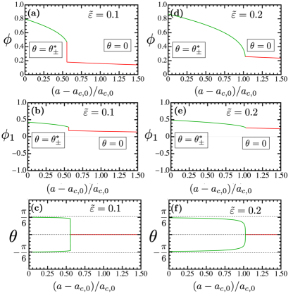
Figure 4: Behavior of the nematic order parameter for fixed $\tilde{\varepsilon}>0$ across the first-order transition line [panels (a), (b), and (c)] and the second-order transition line [panels (d), (e), and (f)], as defined in the phase diagram of Fig. 2. Representative values of $\tilde{\varepsilon}$ are chosen from the left and right side of $\tilde{\varepsilon}_{\text{QTCP}}=3/16\approx 0.19$, respectively. The top panels show the magnitude of the nematic order parameter $\phi$; the middle panels show the nematic component projected along the strain direction, $\phi_{1}=\phi\cos 2\theta$; the bottom panels show the nematic director angle $\theta$. The horizontal axis corresponds to the non-thermal parameter $a$ measured relative to unstrained Potts-nematic transition $a_{c,0}=2/9$. The red curve corresponds to the $\theta=0$ phase whereas the green curve corresponds to the $\theta=\theta_{\pm}^{*}$ phase.

Before analyzing the behavior of Eq. (32), let us discuss the nature of the phase transition from the $\theta_{-}=0$ phase to the $\theta_{\pm}^{*}$ phase. In contrast to the $\tilde{\varepsilon}<0$ case discussed in Sec. II.2, here the emergent Ising degree of freedom $\theta$ is related to a symmetry of the system, namely, twofold rotations with respect to an in-plane axis, $C^{\prime}_{2}$. Indeed, as pointed out in Ref. (Fernandes and Venderbos, 2020), when the director moves away from the high-symmetry directions $p\pi/6$ (with $p=1,\cdots,5$), which is the case only in the $\theta_{\pm}^{*}$ phase, the twofold rotational symmetry $C^{\prime}_{2}$ is spontaneously broken – in addition to the threefold rotational symmetry $C_{3z}$ that is explicitly broken by the external strain.

More formally, focusing on a lattice with point group $\mathrm{D_{6h}}$, strain applied along a high symmetry direction lowers the point group symmetry to $\mathrm{D_{2h}}$. The onset of the $\theta_{\pm}^{*}$ phase breaks the in-plane twofold rotational symmetry, further lowering the point group symmetry to $\mathrm{C_{2h}}$. In the phase diagram of Fig. 2, starting from the $\tilde{\varepsilon}=0$ axis slightly above the nematic transition point ($a>a_{c,0}$) and then increasing $\tilde{\varepsilon}$ (i.e. $\tilde{\varepsilon}>0$), the sequence of point-group-symmetry lowering is $\mathrm{D_{6h}\rightarrow D_{2h}\rightarrow C_{2h}}$. Importantly, while the first symmetry-breaking is explicit and caused by any non-zero $\tilde{\varepsilon}$, the second one is spontaneous and requires a threshold value for $\tilde{\varepsilon}$. In contrast, upon decreasing $\tilde{\varepsilon}$ (i.e. $\tilde{\varepsilon}<0$), there is only the explicit symmetry breaking $\mathrm{D_{6h}\rightarrow D_{2h}}$ caused by a non-zero $\tilde{\varepsilon}$. Following the same steps for the other point groups considered here, we find the following sequences of symmetry lowering upon increasing $\tilde{\varepsilon}$: $\mathrm{D_{3h}\rightarrow C_{2v}\rightarrow C_{s}}$, $\mathrm{D_{3d}\rightarrow C_{2h}\rightarrow S_{2}}$, $\mathrm{D_{6}\rightarrow D_{2}\rightarrow C_{2}}$, and $\mathrm{D_{3}\rightarrow C_{2}\rightarrow C_{1}}$.

This result becomes even more interesting in the case of lattices described by the point groups $\mathrm{D_{6}}$ and $\mathrm{D_{3}}$, which lack any mirror symmetries. These are the groups that describe the symmetries of twisted bilayer graphene and twisted double-bilayer graphene. In these cases, spontaneous breaking of the in-plane twofold rotational symmetry in the $\theta_{\pm}^{*}$ phase results in the condensation of an electric polarization $P_{z}$ pointing out of the plane. This can be seen by analyzing how the Potts-nematic order parameter couples to $P_{z}$ in these groups. Following Ref. (Samajdar et al., 2021), the nemato-electric action is given by:

$$S^{\prime}=\frac{\Upsilon}{6}\,P_{z}\phi^{3}\sin 6\theta=\frac{\Upsilon}{6}\,P_{z}\phi^{3}\sin 6\tilde{\theta}$$ (37)

where $\Upsilon$ is a coupling constant. Expanding for small $\theta$, we find:

$$S^{\prime}\approx\Upsilon\left(\frac{\tilde{\varepsilon}}{3}\right)^{3/2}P_{z}\,\theta$$ (38)

Therefore, a non-zero $\theta$ necessarily triggers a non-zero out-of-plane electric polarization, which allows us to identify the $\theta_{\pm}^{*}$ phase with a ferroelectric phase. However, because this phase is only accessible in the presence of externally applied uniaxial strain, we dub it a piezoelectric phase. We emphasize that the onset of piezoelectricity is a specific property of $\mathrm{D_{6}}$ and $\mathrm{D_{3}}$ lattices only.

The shape of the piezoelectric transition line in the $\left(\tilde{\varepsilon},a\right)$ phase diagram, as well as the character of the transition, can be directly obtained from minimization of Eq. (32). The QTCP takes place for $\mathcal{A}=\mathcal{U}=0$, yielding:

$$a_{\text{QTCP}} =\frac{7}{16}$$ (39)

$$\tilde{\varepsilon}_{\text{QTCP}} =\frac{3}{16}$$ (40)

For $\tilde{\varepsilon}>\tilde{\varepsilon}_{\text{QTCP}}$, the piezoelectric transition is second-order, since $\mathcal{U}>0$. In this regime, the transition line is given by $\mathcal{A}=0$, which corresponds to:

$$a_{c}\left(\tilde{\varepsilon}\right)=\frac{2\sqrt{3\tilde{\varepsilon}}-\tilde{\varepsilon}}{3}\,,\quad\mathrm{for}\;\,\tilde{\varepsilon}>\tilde{\varepsilon}_{\text{QTCP}}\,.$$ (41)

On the other hand, for $0<\tilde{\varepsilon}<\tilde{\varepsilon}_{\text{QTCP}}$, $\mathcal{U}<0$ and the piezoelectric transition is first-order. Minimizing Eq. (32), we find that the first-order transition takes place when the following condition is met:

$$\mathcal{A}=\frac{3\mathcal{U}^{2}}{16\mathcal{W}}$$ (42)

which corresponds to:

$$a_{c}\left(\tilde{\varepsilon}\right)=\frac{-1278\tilde{\varepsilon}+1606\sqrt{3\tilde{\varepsilon}}+\sqrt{15\tilde{\varepsilon}}\sqrt{25344\tilde{\varepsilon}-12312\sqrt{3\tilde{\varepsilon}}+4487}}{2214}\,,\quad\mathrm{for}\;\,0<\tilde{\varepsilon}<\tilde{\varepsilon}_{\text{QTCP}}\,.$$ (43)

Note that this is an approximate expression valid only close to $\tilde{\varepsilon}_{\text{QTCP}}$. In Fig. 4, we show the behavior of different components of the nematic order parameter – the magnitude $\phi$, the projection $\phi_{1}=\phi\cos 2\theta$, and the angle $\theta$ – as a function of the non-thermal tuning parameter for two different values of $\tilde{\varepsilon}>0$. For $\tilde{\varepsilon}<\tilde{\varepsilon}_{\text{QTCP}}$, all components change discontinuously across the piezoelectric transition [Figs. 4(a)-(c)], whereas for $\tilde{\varepsilon}>\tilde{\varepsilon}_{\text{QTCP}}$, all components change continuously [Figs. 4(d)-(f)]. We note that, for large enough $\tilde{\varepsilon}>0$, the derivative of the second-order transition line with respect to $\tilde{\varepsilon}$ changes, as described by Eq. (41), resulting in a reentrance of the $\theta_{+}=0$ phase as a function of strain for fixed $a$. This behavior is not shown in the phase diagram of Fig. 2 because it only happens for very large strain values, $\tilde{\varepsilon}>3$ (for comparison, recall that the nematic order parameter jump across the unstrained Potts-nematic transition is $\Delta\phi_{0}=1/3$).

We finish this section by discussing the properties of the line of piezoelectric QCPs described by Eq. (41). As in the case of the QCEP discussed in the previous section, the dynamical critical exponent is $z=1$ in the case of an insulator. For a metallic system, we start from the action (25), substitute $\phi_{q}=\sqrt{\frac{\tilde{\varepsilon}}{3}}$ and expand for small $\theta$ to obtain:

$$\mathcal{S}_{\text{int}}=\sqrt{\frac{4\tilde{\varepsilon}}{3}}\,g\int_{k,q}\theta_{q}\sin\left(2\tilde{\beta}_{\mathbf{k}}\right)\psi_{k+q/2}^{\dagger}\psi_{k-q/2}^{\phantom{}}$$ (44)

where, as before, $\tilde{\beta}_{\mathbf{q}}=\beta_{\mathbf{q}}-\alpha$. Note that the electronic dispersion is also renormalized due to the external strain, $\xi_{\mathbf{k}}=\xi_{0,\mathbf{k}}+\sqrt{\frac{\tilde{\varepsilon}}{3}}\,g\cos\left(2\tilde{\beta}_{\mathbf{k}}\right)$. Like the QCEP case studied in Sec. II.2, the form factor in Eq. (44) is that of an Ising-nematic QCP. Interestingly, the two Ising-nematic form factors in Eqs. (26) and (44) are “orthogonal” in the nematic space, corresponding to the longitudinal and transverse modes of a hypothetical XY nematic order parameter (Oganesyan et al., 2001; Garst and Chubukov, 2010). This is a consequence of the fact that, for $\tilde{\varepsilon}<0$, the nematic director angle is pinned and the nematic amplitude is fluctuating, whereas for $\tilde{\varepsilon}>0$ it is $\theta$ that fluctuates.

To one-loop order, the polarization bubble is given by:

$$\Pi(q)=-\frac{8}{3}\,\tilde{\varepsilon}g^{2}\int_{k}\sin^{2}\left(2\tilde{\beta}_{\mathbf{k}}\right)G_{0,k+q/2}G_{0,k-q/2}$$ (45)

which evaluates to:

$$\delta\Pi(q) =-\frac{\tilde{\varepsilon}g^{2}}{2E_{F}}\,f_{3}\left(\frac{g}{E_{F}}\sqrt{\frac{\tilde{\varepsilon}}{3}},\cos 2\tilde{\beta}_{\mathbf{q}}\right)\frac{|\Omega|}{v_{F}|\mathbf{q}|}$$

$$-\frac{\tilde{\varepsilon}g^{2}}{2E_{F}}\,f_{4}\left(\frac{g}{E_{F}}\sqrt{\frac{\tilde{\varepsilon}}{3}},\cos 2\tilde{\beta}_{\mathbf{q}}\right)\left(\frac{\Omega}{v_{F}|\mathbf{q}|}\right)^{2}$$ (46)

where we defined the functions:

$$f_{3}(\tilde{g},x) =\frac{4}{3\pi}\frac{1-x^{2}}{\sqrt{1-\tilde{g}^{2}}(1+\tilde{g}x)^{5/2}}$$ (47)

$$f_{4}(\tilde{g},x) =\frac{4}{3\pi}\frac{3\tilde{g}^{2}+4\tilde{g}x+(2-\tilde{g}^{2})(2x^{2}-1)}{(1-\tilde{g}^{2})^{3/2}(1+\tilde{g}x)^{3}}$$ (48)

Thus, within a Hertz-Millis approximation for the dynamical critical exponent $z$, we find $z=3$, except for the cold spots parametrized by $f_{3}\left(x_{\mathrm{cs}}\right)=0$, for which $z=2$. The last result follows from the fact that, since $\tilde{g}$ is small, $f_{4}\left(x_{\mathrm{cs}}\right)>0$. Moreover, note that $f_{3}\left(x\right)\geq 0$ for any $x$. Interestingly, in contrast to the QCEP case, here the cold spots are the same as in the case of the undistorted Fermi surface, $\tilde{\beta}_{\mathbf{q}}=0,\text{ }\pi/2$. This can be understood geometrically by noting that the semi-major axes of the elliptical Fermi surface coincide with its cold spots. As a result, cold-spot fermions at $\beta_{\mathbf{k}}=0$ ($\beta_{\mathbf{k}}=\pi/2$) will necessarily exchange underdamped collective bosons with momentum direction $\tilde{\beta}_{\mathbf{q}}=\pi/2$ ($\tilde{\beta}_{\mathbf{q}}=0$).

III Hysteresis and spinodal lines

The phase boundaries in the phase diagram of Fig. 2 were obtained by determining the global minimum of the action. In the case of first-order transitions, however, the action also has local minima, which correspond to metastable phases. While they are formally inaccessible in true equilibrium, they can be probed via hysteresis measurements in which the order parameter $\boldsymbol{\Phi}$ is measured upon cycling the conjugate field $\tilde{\varepsilon}$. The interesting aspect of the Potts-nematic state is that the action has three discrete minima rather than two, which should lead to more complex hysteresis loops as compared to the standard Ising-nematic case.

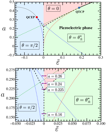
Figure 5: The zero temperature phase diagram of Fig. 2 is shown with the spinodal lines included (top panel). The two blue dashed lines on the left side ($\tilde{\varepsilon}<0$) are the upper and lower spinodals corresponding to the two phases associated with the meta-nematic transition. They coincide at the QCEP. The green and red dashed curves on the right side ($\tilde{\varepsilon}>0$) are the upper and lower spinodals of the $\theta=\theta_{\pm}^{*}$ (piezoelectric) and $\theta=0$ phases, respectively. They coincide at the QTCP. The bottom panel is a zoom of the top panel; the purple arrows show the values of $a$ for which the hysteresis curves $\boldsymbol{\Phi}\left(\tilde{\varepsilon}\right)$ in Fig. 6 are shown.

To calculate these hysteresis curves, we first derive the upper and lower spinodals associated with the first-order transition lines in Fig. 2. As in Sec. II, we consider $\lambda>0$ and drop the tilde of the rescaled variables (except for $\tilde{\varepsilon}$). The spinodals are curves on the $(\tilde{\varepsilon},a)$-plane that bound the regions of metastability of the different phases. We consider first the phase $\theta_{-}=\pi/2$; it corresponds to a local minimum as long as the following metastability conditions are met

$$\partial_{\phi}S_{\text{nem}}(\theta=\pi/2)=\phi^{3}-\phi^{2}+a\phi+\tilde{\varepsilon}=0$$ (49)

$$\begin{cases}\partial_{\phi}^{2}S_{\text{nem}}(\theta=\pi/2)=3\phi^{2}-2\phi+a>0\\ \partial_{\theta}^{2}S_{\text{nem}}(\theta=\pi/2)=3\phi^{3}-\tilde{\varepsilon}\phi>0\end{cases}$$ (50)

Since $\partial_{\theta}\partial_{\phi}S_{\text{nem}}$ vanishes, positive-definiteness of the Hessian matrix of second derivatives $\left(\partial_{i}\partial_{j}S_{\text{nem}}\right)$ is ensured by Eq. (50). It is convenient to define the cubic discriminant of Eq. (49), $\mathcal{D}_{\pi/2}=a^{2}-4a^{3}+4\tilde{\varepsilon}-27\tilde{\varepsilon}^{2}-18a\varepsilon$. When $\mathcal{D}_{\pi/2}<0$, Eq. (49) has only one real $\phi$ solution, whereas when $\mathcal{D}_{\pi/2}>0$, there are three real $\phi$ solutions. In the latter case, $\mathcal{D}_{\pi/2}>0$, the largest and smallest values of $\phi$ that solve Eq. (49) correspond to the two solutions associated with the meta-nematic transition. On the other hand, in the former case, $\mathcal{D}_{\pi/2}<0$, the single real solution indicates that there is no meta-nematic transition, as is the case to the left of the QCEP. This suggests that $\mathcal{D}_{\pi/2}=0$ gives the spinodals associated with the meta-nematic transition. There is, however, one subtlety: by construction, $\phi$ must be positive. Therefore, it is not enough to ensure the existence of a real solution, but of a real and positive solution. It turns out that, when $\tilde{\varepsilon}<0$, the real solutions of Eq. (49) in both cases ($\mathcal{D}_{\pi/2}>0$ and $\mathcal{D}_{\pi/2}<0$) are always positive. However, when $\tilde{\varepsilon}>0$, the single solution in the $\mathcal{D}_{\pi/2}<0$ case is negative, whereas only one among the two positive solutions in the $\mathcal{D}_{\pi/2}>0$ case is an action minimum. Taking these conditions into account and solving the equation $\mathcal{D}_{\pi/2}=0$ for $a$, we find the equations describing the spinodals of the meta-nematic transition. The three solutions of $\mathcal{D}_{\pi/2}=0$ can be written as:

$$a_{n}(\tilde{\varepsilon}) =\frac{1}{12}\Big{(}1-\mathrm{e}^{2ni\pi/3}\,b(\tilde{\varepsilon})+\mathrm{e}^{-2ni\pi/3}\,\frac{216\tilde{\varepsilon}-1}{b(\tilde{\varepsilon})}\Big{)}\,,$$ (51)

$$b(\tilde{\varepsilon}) =\big{[}108\tilde{\varepsilon}(54\tilde{\varepsilon}-5)+24\sqrt{3\tilde{\varepsilon}(27\tilde{\varepsilon}+1)^{3}}-1\big{]}^{\frac{1}{3}}$$ (52)

with $n=0,1,2$. Then, the upper spinodal is given by:

$$a_{\text{us}}^{\text{meta}}(\tilde{\varepsilon})=\left\{\begin{array}[]{ll}a_{1}(\tilde{\varepsilon})&\,,\quad\mathrm{for}\;\,\tilde{\varepsilon}_{\text{QCEP}}<\tilde{\varepsilon}<\tilde{\varepsilon}_{*}\\ a_{0}(\tilde{\varepsilon})&\,,\quad\mathrm{for}\;\,\tilde{\varepsilon}>\tilde{\varepsilon}_{*}\end{array}\right.$$ (53)

with $\tilde{\varepsilon}_{*}=1/216$ defined such that $b\left(\tilde{\varepsilon}_{*}\right)=0$. For the lower spinodal, we obtain:

$$a_{\text{ls}}^{\text{meta}}(\tilde{\varepsilon})=a_{2}(\tilde{\varepsilon})\,,\quad\mathrm{for}\;\,\tilde{\varepsilon}_{\text{QCEP}}<\tilde{\varepsilon}<0\,$$

Here, the subscripts “us” and “ls” denote upper spinodal and lower spinodal, respectively. In particular, $a_{\text{us}}^{\text{meta}}(\tilde{\varepsilon})$ giv es the limit of metastability of the $\theta_{-}$ phase below the meta-nematic transition line, whereas $a_{\text{ls}}^{\text{meta}}(\tilde{\varepsilon})$ gives the limit of metastability of the $\theta_{-}$ phase above the meta-nematic transition line. These spinodal lines are shown by the blue dashed lines in the phase diagram of Fig. 5.

We now analyze the metastability of the $\theta_{+}=0$ phase. The metastability conditions are given by:

$$\partial_{\phi}S_{\text{nem}}(\theta=0)=\phi^{3}+\phi^{2}+a\phi-\tilde{\varepsilon}=0$$ (54)

$$\begin{cases}\partial_{\phi}^{2}S_{\text{nem}}(\theta=0)=3\phi^{2}+2\phi+a>0\\ \partial_{\theta}^{2}S_{\text{nem}}(\theta=0)=-3\phi^{3}+\tilde{\varepsilon}\phi>0.\end{cases}$$ (55)

Applying a similar analysis as in the $\theta_{-}=\pi/2$ case, we find that $\theta_{+}=0$ ceases to be a local minimum when the second condition of Eq. (55) fails. Plugging in $\phi^{2}=\tilde{\varepsilon}/3$ into Eq. (54), we find:

$$a_{\text{ls}}^{\text{piezo}}(\tilde{\varepsilon})=\frac{2\sqrt{3\tilde{\varepsilon}}-\tilde{\varepsilon}}{3}\,,\quad\mathrm{for}\;\,0<\tilde{\varepsilon}<\tilde{\varepsilon}_{\text{QTCP}}$$ (56)

which corresponds to the lower spinodal of the first-order piezoelectric phase transition, shown by the dashed red line in the phase diagram of Fig. 5. To obtain the upper spinodal of this transition, we need to analyze the metastability of the $\theta=\theta_{\pm}^{*}$ phase. Eq. (3) gives the nematic magnitude $\phi_{+}^{*}$ in the $\theta_{\pm}^{*}$ phase. For $\tilde{\varepsilon}<\tilde{\varepsilon}_{\text{QTCP}}$, the condition $(\phi_{+}^{*})^{2}\geq\tilde{\varepsilon}/3$ required for $\theta_{\pm}^{*}$ in Eq. (12) to exist is always satisfied. Moreover, the $\phi_{+}^{*}$ solution exists as long as the argument of the square root in Eq. (3) is positive, $a<\tilde{\varepsilon}+1/4$. This therefore defines the limit of metastability of the $\theta_{\pm}^{*}$ phase, which corresponds to the upper spinodal of the first-order piezoelectric transition. It is shown by the dashed green line in Fig. 5(a) and given by:

$$a_{\text{us}}^{\text{piezo }}(\tilde{\varepsilon})=\tilde{\varepsilon}+\frac{1}{4}\,,\quad\mathrm{for}\;\,\tilde{\varepsilon}<\tilde{\varepsilon}_{\text{QTCP}}$$ (57)

Interestingly, for $\tilde{\varepsilon}>\tilde{\varepsilon}_{\text{QTCP}}$, the condition $(\phi_{+}^{*})^{2}\geq\tilde{\varepsilon}/3$ would imply an upper spinodal $a_{\text{us}}^{\text{piezo }}(\tilde{\varepsilon})=\frac{2\sqrt{3\tilde{\varepsilon}}-\tilde{\varepsilon}}{3}$, which is identical to what the lower spinodal would be in this strain range, see Eq. (56). The coincidence between the upper and lower spinodals implies that the transition is actually second-order. Indeed, these would-be spinodals have the same expression as the one describing the second-order transition line, Eq. (41).

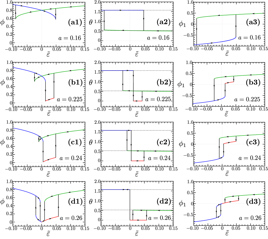
Figure 6: Hysteresis curves of the nematic order parameter as a function of uniaxial strain $\tilde{\varepsilon}$ for four representive values of $a$ marked by the purple arrows in Fig. 5. Panels (a) correspond to $a=0.16$; (b), to $a=0.225$; (c), to $a=0.24$; and (d), to $a=0.26$. Left, middle, and right panels, which are identified by the numbers 1, 2, and 3, respectively, correspond to the nematic magnitude $\phi$, the nematic director angle $\theta$, and the nematic component projected along the direction of the strain, $\phi_{1}=\phi\cos 2\theta$. Red, green, and blue colors denote the action minimum $\theta=0$, $\theta=\theta_{\pm}^{*}$, and $\theta=\pi/2$, respectively.

We are now in position to analyze the hysteresis curves $\boldsymbol{\Phi}\left(\tilde{\varepsilon}\right)$ as the strain $\tilde{\varepsilon}$ is cycled. We employ the Stoner-Wohlfarth approach (Stoner and Wohlfarth, 1948): starting deep in one of the ordered states, we assume that the system remains in this state until it is no longer a local minimum of the action, i.e. until its spinodal line is crossed, at which point the system moves to another minimum. In the Ising-nematic case, this last step is straightforward, as there is only one minimum available in the action landscape after the spinodal line is crossed. However, in the Potts-nematic case, there can be two local minima. To decide which of the two minima the system chooses, we employ a “gradient-descent criterion.” Specifically, we introduce a “time” variable $s$, promoting $\boldsymbol{\Phi}$ to a dynamical field $\boldsymbol{\Phi}(s)$, and define a generalized gradient-descent equation:

$$\dot{\phi}_{i}=-\eta_{ij}\frac{\partial S_{\text{nem}}}{\partial\phi_{j}},$$ (58)

where, we recall, $\boldsymbol{\Phi}\equiv\left(\phi_{1},\,\phi_{2}\right)=\phi\left(\cos 2\theta,\,\sin 2\theta\right)$. Here, repeated indices are implicitly summed, $\dot{\phi}_{i}=\partial\phi_{i}/\partial s$, and $\eta_{ij}$ is a positive-definite matrix. The last condition ensures that Eq. (58) remains purely diffusive, such that $\boldsymbol{\Phi}$ approaches a local minimum of $S_{\text{nem}}$ as $s\to\infty$. We set $\eta_{ij}=\eta\delta_{ij}$ with $\eta>0$, in which case solutions to Eq. (58) are trajectories of steepest descent. We rescale $s\to s^{\prime}=s/\eta$ and redefine $\dot{\phi}_{i}=\partial\phi_{i}/\partial s^{\prime}$ to obtain the autonomous system

$$\begin{cases}\dot{\phi}_{1}&=-a\phi_{1}-\phi_{1}(\phi_{1}^{2}+\phi_{2}^{2})-(\phi_{1}^{2}-\phi_{2}^{2})+\tilde{\varepsilon}\\ \dot{\phi}_{2}&=-a\phi_{2}-\phi_{2}(\phi_{1}^{2}+\phi_{2}^{2})+2\phi_{1}\phi_{2}\end{cases}$$ (59)

The procedure we adopt once the system approaches a spinodal at $\tilde{\varepsilon}^{*}$, for a fixed $a$ value, is as follows: let $\tilde{\varepsilon}^{+}$ and $\tilde{\varepsilon}^{-}$ be strain values near $\tilde{\varepsilon}^{*}$ and within the unstable and stable sides of the spinodal curve, respectively. Let $\boldsymbol{\Phi}_{\text{min}}^{(\tilde{\varepsilon}^{-})}$ be the local minimum of the action at $\tilde{\varepsilon}=\tilde{\varepsilon}^{-}$, which disappears once $\tilde{\varepsilon}=\tilde{\varepsilon}^{+}$. We then set $\tilde{\varepsilon}=\tilde{\varepsilon}^{+}$ in Eq. (59) and choose several initial conditions $\boldsymbol{\Phi}(0)$ in a narrow neighborhood of $\boldsymbol{\Phi}_{\text{min}}^{(\tilde{\varepsilon}^{-})}$, $|\boldsymbol{\Phi}(0)-\boldsymbol{\Phi}_{\text{min}}^{(\tilde{\varepsilon}^{-})}|\lesssim 10^{-4}$, letting the system evolve until a new local minima is encountered. We found that $\boldsymbol{\Phi}(s)$ approaches the same minimum for all initial conditions we investigated, which suggests that the outcome is insensitive to any initial condition within a small vicinity of $\boldsymbol{\Phi}_{\text{min}}^{(\tilde{\varepsilon}^{-})}$.

We applied this procedure to four representative fixed values of $a$ in the phase diagram of Fig. 5, marked by the purple arrows in the bottom panel. They each correspond to one of the four regions bounded by the values of $a$ in which two different spinodal lines intersect, namely:

$$\begin{cases}a_{1}&=-39+16\sqrt{6}\approx 0.1918\\ a_{2}&=\frac{-45+13\sqrt{13}}{8}\approx 0.2340\\ a_{3}&=a_{\text{us}}^{\text{Potts}}=0.25.\end{cases}$$ (60)

Here, $a_{1}$ corresponds to the crossing between the blue and red dashed spinodal lines; $a_{2}$ corresponds to the lower crossing between the blue and green dashed spinodal lines; and $a_{3}$ corresponds to the upper crossing between the blue and green dashed spinodal lines, which also coincides with the upper spinodal of the unstrained Potts transition.

The hysteresis curves for the four representative $a$ values marked in 5 are shown in Fig. 6. In this figure, we present the hysteresis curves for the nematic magnitude $\phi\left(\tilde{\varepsilon}\right)$, the nematic director angle $\theta\left(\tilde{\varepsilon}\right)$, and the nematic component projected along the strain direction, $\phi_{1}=\phi\cos 2\theta$. Panels (a1)-(a3) show the case $a=0.16<a_{1}$. The system starts deep inside the $\theta_{\pm}^{*}$ green phase (piezoelectric phase) when $\tilde{\varepsilon}$ is large and positive. Upon decreasing $\tilde{\varepsilon}$ (from right to left in Fig. 6(a1)-(a3)), the system remains in the metastable $\theta_{\pm}^{*}$ phase until it reaches the dashed green spinodal line, where $\tilde{\varepsilon}<0$. At this point, the only available minimum is the $\theta_{-}=\pi/2$ blue phase below the meta-nematic transition. Once we reverse $\tilde{\varepsilon}$ and start increasing it (from left to right in Fig. 6(a1)-(a3)), the system remains in the $\theta_{-}=\pi/2$ phase until the spinodal blue dashed line is crossed in the $\tilde{\varepsilon}>0$ side of the phase diagram, at which point the system moves back to the $\theta_{\pm}^{*}$ green phase. In terms of the $\phi_{1}$ component, the hysteresis curve is a rather standard one, albeit not symmetric with respect to either the $\phi_{1}$ or the $\tilde{\varepsilon}$ axes.

Fig. 6(b1)-(b3) shows the hysteresis curves for the case $a_{1}<a=0.225<a_{2}$. Starting deep from the $\tilde{\varepsilon}>0$ side of the phase diagram and then decreasing $\tilde{\varepsilon}$ (i.e. going from right to left in the plots), the situation is the same as in panels (a1)-(a3), namely, the system remains in the $\theta_{\pm}^{*}$ green phase until the green spinodal line is crossed on the $\tilde{\varepsilon}<0$ side of the phase diagram. However, upon reversing $\tilde{\varepsilon}$ and increasing it (i.e. going from left to right in the plots), the situation changes. Once the blue dashed spinodal line is crossed, on the $\tilde{\varepsilon}>0$ side of the phase diagram, there are two local minima available: the global minimum corresponding to the $\theta_{\pm}^{*}$ green phase and the metastable minimum corresponding to the $\theta_{+}=0$ red phase. By solving Eq. (58), we find that the system moves to the $\theta_{+}=0$ red phase and remains at this local minimum until the red dashed spinodal line is crossed, at which point the system finally moves back to the $\theta_{\pm}^{*}$ green phase. This behavior results in multi-loop hysteresis curves.

The case $a_{2}<a=0.24<a_{3}$ is depicted in Fig. 6(c1)-(c3). The behavior upon increasing $\tilde{\varepsilon}$ (i.e. going from left to right in the plots) is the same as in panels (b1)-(b3). On the other hand, the sequence of spinodals crossed upon decreasing $\tilde{\varepsilon}$ (i.e. going from right to left in the plots) is different: once the green dashed spinodal line is crossed, there are now two local minima available, corresponding to the two $\theta_{-}=\pi/2$ blue phases associated with the two sides of the meta-nematic transition. The solution of Eq. (58) shows that the system moves to the global minimum, where it remains as $\tilde{\varepsilon}$ continues being decreased. Therefore, although the sequence of spinodals crossed is different from the case of panels (b1)-(b3), the sequence of metastable phases probed is the same.

Finally, Fig. 6(d1)-(d3) shows the case $a=0.26>a_{3}$. Upon decreasing $\tilde{\varepsilon}$ (right to left in the plots), the green dashed spinodal line is now crossed on the $\tilde{\varepsilon}>0$ side of the phase diagram. The only available minimum is the $\theta_{+}=0$ phase, which however ceases to be a solution once the $\tilde{\varepsilon}=0$ line is crossed. At this axis, $\phi\rightarrow 0$, which is a consequence of the fact that the system is above the upper spinodal $a_{3}$ of the unstrained Potts-nematic transition. The system then moves to the $\theta_{-}=\pi/2$ blue phase above the meta-nematic transition, where it remains until the lower blue dashed spinodal line is crossed. At this point, the system moves to the $\theta_{-}=\pi/2$ blue phase below the meta-nematic transition. The behavior upon increasing $\tilde{\varepsilon}$ (left to right in the plots) can be understood in a similar manner. The resulting hysteresis curves display multiple loops, which however do not cross the origin, since $\phi=0$ when $\tilde{\varepsilon}=0$.

IV Non-zero-temperature phase diagram

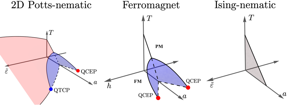
Figure 7: Left panel: Qualitative $(\tilde{\varepsilon},a,T)$ phase diagram of a 2D Potts-nematic system (same as Fig. 1). Middle panel: $(h,a,T)$ phase diagram of an itinerant ferromagnet, where $h$ is the magnetic field (see Refs. (Belitz et al., 2005; Brando et al., 2016)). The first-order wings are symmetric with respect to $h$ and are bounded by a line of classical critical end-points terminating at QCEPs. Right panel: $(\tilde{\varepsilon},a,T)$ phase diagram of an Ising-nematic system. There is a second-order transition only along the $\tilde{\varepsilon}=0$ plane. Any non-zero strain along the nematic director directions smears the transition completely.

At $T=0$, the Potts-nematic phase diagram is expected to be the same for both 2D and 3D systems, since in either case the effective dimensionality $d+z$ is larger than the upper critical dimension of the 3-state Potts model, $d_{u}^{\mathrm{Potts}}\lesssim 3$, such that a mean-field analysis is warranted. At larger temperatures, where the bosonic quantum dynamics can be neglected, the situation is different. Since $d=3>d_{u}^{\mathrm{Potts}}$, in the 3D case the $\left(\tilde{\varepsilon},a,T\right)$ phase diagram consists essentially of a sequence of “copies” of the phase diagram shown in Fig. 2. Similarly, for a fixed $a$, the $\left(\tilde{\varepsilon},T\right)$ phase diagram has the same form as the one obtained at $T=0$, but with the $y$-axis representing $T-T_{c}$.

The situation at non-zero temperatures is more interesting in the 2D case. The fact that $d=2<d_{u}^{\mathrm{Potts}}$ implies that the mean-field solution is not applicable. Surprisingly, despite the presence of a cubic invariant in the free energy expansion, the 2D 3-state Potts model undergoes a second-order transition characterized by the critical exponents $\alpha=1/3$ and $\beta=1/9$, which are in the universality class of the hard hexagon lattice gas model (Wu, 1982). Of course, one cannot exclude the possibility that for particular microscopic models the quartic Landau coefficient is negative, rendering the transition first-order. But, in the general case, we expect that, in the absence of strain and at high enough temperatures, the Potts-nematic transition is second-order. As a result, since at $T=0$ the Potts-nematic transition is first-order, the $(a,T)$ phase diagram with fixed $\tilde{\varepsilon}=0$ should display a (classical) tricritical point. It is difficult to estimate the position of this tricritical point, since standard perturbative approaches such as renormalization-group calculations do not capture the second-order character of the transition in 2D. It would be interesting to perform Monte Carlo simulations to pinpoint the position of the classical tricritical point.

Having established the $\left(\tilde{\varepsilon},a\right)$ phase diagram at $T=0$ and the $(a,T)$ phase diagram at $\tilde{\varepsilon}=0$, we can conjecture the full qualitative three-dimensional $\left(\tilde{\varepsilon},a,T\right)$ phase diagram for the 2D Potts-nematic model by continuously connecting the QTCP and the QCEP at $T=0$ with the classical tricritical point at $\tilde{\varepsilon}=0$. The result, shown in Fig. 1 and repeated for convenience in the left panel of Fig. 7, consists of two wings (in blue) inside which the transition is first-order. On the $\tilde{\varepsilon}<0$ side, the wing is isolated and the transition is a symmetry-preserving meta-nematic one. On the other hand, on the $\tilde{\varepsilon}>0$ side, the wing is connected to a larger surface (in red) that signals a second-order transition. Regardless of the character of the transition in the $\tilde{\varepsilon}>0$ region, it is associated with the spontaneous breaking of an in-plane twofold rotational symmetry, which is manifested as a piezoelectric phase in the case of twisted moiré systems.

It is interesting to compare this $\left(\tilde{\varepsilon},a,T\right)$ phase diagram with that expected for an Ising-nematic order parameter, as realized in tetragonal lattices. As shown in the right panel of Fig. 7, in the Ising-nematic case the system is generically expected to undergo a second-order transition only along the $\tilde{\varepsilon}=0$ plane. Any strain applied along the directions of the nematic director completely smears the Ising-nematic phase transition. This is what renders it difficult to unambiguously distinguish spontaneous Ising-nematic order from strain-induced anisotropies in experimental settings, where residual strain is invariably present. In contrast, meta-nematic and piezoelectric transitions persist for a wide range of strain values in the case of Potts-nematic order. Experimental observation of these effects would provide direct evidence for spontaneous Potts-nematic order.

The wings in the $\left(\tilde{\varepsilon},a,T\right)$ phase diagram of the Potts-nematic order, bounded by tricritical points and critical end-points, are reminiscent of the wings generally expected in the $\left(h,a,T\right)$ phase diagram of a metallic (Heisenberg) ferromagnet, which is schematically shown in the middle panel of Fig. 7 (see Refs. (Belitz et al., 2005; Brando et al., 2016)). Note that here $h$ denotes a magnetic field. At first sight, this analogy may seem unsurprising, since both $\tilde{\varepsilon}$ and $h$ act as conjugate fields to the nematic and ferromagnetic order parameters, respectively. However, there are crucial qualitative differences. First, because the nematic order parameter is 3-state Potts-like rather than continuous, there is a fundamental asymmetry between the effects of compressive strain and tensile strain, whereas in the ferromagnetic case the phase diagram is symmetric with respect to the sign of the magnetic field. Second, the mechanisms behind the first-order $T=0$ transitions are completely different in the two cases. In the Potts-nematic case, the first-order nature of the quantum phase transition is an intrinsic property of the bosonic model, as it is a direct consequence of it being above its upper critical dimension. In contrast, in the metallic ferromagnetic case, the $T=0$ transition is rendered first-order due to the coupling between the ferromagnetic Goldstone modes and the gapless electron-hole excitations of the metal (Belitz et al., 1999; Chubukov et al., 2004; Maslov and Chubukov, 2009).

V Conclusions

In this paper, we used a phenomenological approach to establish the $\left(\tilde{\varepsilon},a,T\right)$ phase diagram of the electronic 3-state Potts-nematic model in the presence of uniaxial strain applied along one of the high-symmetry directions of a lattice that possesses out-of-plane threefold rotational symmetry and in-plane twofold rotational symmetry. While $a$ is a non-thermal tuning parameter, such as doping, the parameter $\tilde{\varepsilon}$ is linearly proportional to the applied strain. Whether compressive or tensile strain gives $\tilde{\varepsilon}<0$ or $\tilde{\varepsilon}>0$ depends on the signs of the cubic nematic coefficient and the nemato-elastic coupling. At zero temperature and zero strain, the mean-field approach is justified due to the reduced upper critical dimension of the 3-state Potts model, $d_{u}^{\mathrm{Potts}}\lesssim 3$. Then, because the Potts-nematic action contains a cubic invariant, there is no Potts-nematic QCP, but rather a first-order Potts-nematic quantum phase transition. Upon increasing the temperature, but keeping the strain zero, the mean-field solution ceases to be valid in the case of a 2D lattice, and the Potts-nematic transition becomes second-order. Thus, a classical tricritical nematic point is generally expected in an unstrained 2D system, whereas in a 3D system the Potts-nematic transition should be always first-order.

Notwithstanding the absence of a QCP in an unstrained 2D or 3D system, application of strain can tune the system across a a meta-nematic QCEP, for $\tilde{\varepsilon}<0$, and a QTCP followed by a line of QCPs for $\tilde{\varepsilon}>0$. The former transition is symmetry-preserving, whereas the latter spontaneously breaks the in-plane twofold rotational symmetry of the lattice. Note that a non-zero $\tilde{\varepsilon}$ explicitly breaks the out-of-plane threefold rotational symmetry. In lattices with $\mathrm{D_{3}}$ and $\mathrm{D_{6}}$ point-group symmetries, which is the case for instance of twisted bilayer graphene (TBG) and twisted double-bilayer graphene (TDBG), the transition in the $\tilde{\varepsilon}>0$ side of the phase diagram leads to the emergence of a non-zero electric polarization, resulting in what we dubbed a piezoelectric phase – since the ferroelectric order requires the presence of external strain. Connecting the phase diagrams at zero strain and at zero temperature, we proposed the $\left(\tilde{\varepsilon},a,T\right)$ phase diagram for a 2D Potts-nematic system shown in Fig. 1. One of its key features is the existence of two first-order transition wings, bounded by a line of tricritical points in the $\tilde{\varepsilon}>0$ side of the phase diagram, and by a line of critical end-points in the $\tilde{\varepsilon}<0$ side. While the latter wing is isolated, the former is connected to an open surface of second-order phase transitions towards the piezoelectric phase. The recent observation of electronic nematicity in TBG (Kerelsky et al., 2019; Jiang et al., 2019; Choi et al., 2019; Cao et al., 2021), TDBG (Rubio-Verdú et al., 2022), and twisted trilayer graphene (Zhang et al., 2022), which are 2D materials, indicate not only that the phase diagram of Fig. 1 may be realized in moiré superlattices, but also that strain can be used to move the system towards nematic quantum criticality. Note that this is a different mechanism from that proposed in Ref. (Parker et al., 2021) to strain-tune TBG across a quantum phase transition.

It is interesting to contrast the results obtained here for the Potts-nematic phase with those for an Ising-nematic phase, which is realized in lattices with fourfold rotational symmetry. In the Ising-nematic case, “longitudinal” strain applied along either of the two allowed nematic director directions smears the second-order phase transition. However, “transverse” strain applied along the other two high-symmetry directions not encompassed by the nematic director can tune the system towards an Ising-nematic QCP (Maharaj et al., 2017). This offers an interesting insight into why strain is capable of tuning the system across a Potts-nematic QCP. For the lattices considered here, the nematic director can point along any of the high-symmetry lattice directions. Thus, uniaxial strain applied along these directions can have either a “longitudinal” or a “transverse” character, depending on whether strain is compressive or tensile. This asymmetry between compressive and tensile strain traces back to the well-understood inequivalence between positive and negative conjugate fields in the mean-field solution of the 3-state Potts model (Straley and Fisher, 1973; Blankschtein and Aharony, 1980).

The Potts-nematic QCPs that emerge in the presence of strain behave analogously to an Ising-nematic QCP in the absence of strain. In both the $\tilde{\varepsilon}>0$ and $\tilde{\varepsilon}<0$ sides of the phase diagram, the two-component Potts-nematic order parameter is effectively reduced to a single-component one by the external strain, either because the nematic amplitude jumps between two non-zero values while the nematic director angle is pinned by the strain ($\tilde{\varepsilon}<0$), or because the nematic director unlocks from the strain direction by rotating along the clockwise or the counterclockwise direction ($\tilde{\varepsilon}>0$). In fact, under these conditions, the Potts-nematic electronic form factor reduces to the well-known “$\mathrm{B_{1g}}$” Ising-nematic form factor for $\tilde{\varepsilon}<0$ and “$\mathrm{B_{2g}}$” Ising-nematic form factor for $\tilde{\varepsilon}>0$. Consequently, while the QCPs on the two sides of the phase diagram have the same Hertz-Millis dynamical critical exponent $z=3$ except for a few cold spots, for which $z=2$, these cold spots are at different locations depending on the sign of $\tilde{\varepsilon}$. More broadly, the strain-induced Potts-nematic QCPs should support the same phenomena expected for the Ising-nematic QCP, such as superconductivity and non-Fermi liquid behavior (Metlitski and Sachdev, 2010; Metlitski et al., 2015; Schattner et al., 2016; Lederer et al., 2017; Klein et al., 2018; Lee, 2018).

Our results provide valuable criteria to experimentally identify intrinsic Potts-nematic order and distinguish it from extrinsic effects via a controlled application of uniaxial strain. Observation of the characteristic multi-loop hysteresis curves shown in Fig. 6 would be a direct confirmation not only of long-range nematic order, but also of the Potts-like character of the order parameter. Experimentally, $\phi_{1}$ can be probed via resistivity anisotropy measurements similarly to those carried out in the pnictides (Chu et al., 2012). In this regard, as pointed out in Ref. (Vafek, 2022), the geometry used to measured the resistivity plays an important role in extracting the anisotropic component of the resistivity tensor (see also Ref. (Wang et al., 2022a)). Moreover, the observation of a piezoelectric effect in twisted moiré systems that only emerges for one type of strain (compressive or tensile) would provide unambiguous evidence for an intrinsic Potts-nematic instability. Interestingly, ferroelectricity has been recently observed in a moiré heterostructure (Zheng et al., 2020). While in this paper we focused only on externally-applied uniform strain, any crystalline system will invariably be subjected to internal random strain (Carlson et al., 2006; Carlson and Dahmen, 2011; Meese et al., 2022). Given the non-trivial impact of uniform strain on the Potts-nematicity, it will be interesting for future studies to shed light on the properties of the 3-state Potts-nematic model in the presence of both random strain and uniform strain.