Towards Space Efficient Two-Point Shortest Path Queries in a Polygonal Domain

Towards Space Efficient Two-Point Shortest Path Queries in a Polygonal Domain

Abstract

We devise a data structure that can answer shortest path queries for two query points in a polygonal domain $P$ on $n$ vertices. For any $\varepsilon>0$, the space complexity of the data structure is $O(n^{10+\varepsilon})$ and queries can be answered in $O(\log n)$ time. Alternatively, we can achieve a space complexity of $O(n^{9+\varepsilon})$ by relaxing the query time to $O(\log^{2}n)$. This is the first improvement upon a conference paper by Chiang and Mitchell [16] from 1999. They present a data structure with $O(n^{11})$ space complexity and $O(\log n)$ query time. Our main result can be extended to include a space-time trade-off. Specifically, we devise data structures with $O(n^{9+\varepsilon}/\hskip 1.0pt\ell^{4+O(\varepsilon)})$ space complexity and $O(\ell\log^{2}n)$ query time, for any integer $1\leq\ell\leq n$.

Furthermore, we present improved data structures with $O(\log n)$ query time for the special case where we restrict one (or both) of the query points to lie on the boundary of $P$. When one of the query points is restricted to lie on the boundary, and the other query point is unrestricted, the space complexity becomes $O(n^{6+\varepsilon})$. When both query points are on the boundary, the space complexity is decreased further to $O(n^{4+\varepsilon})$, thereby improving an earlier result of Bae and Okamoto [8].

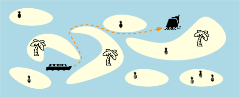
Figure 1: A tangible example of a two-point shortest path problem: finding the shortest path among islands for a boat to an emergency.

1 Introduction

In the two-point shortest path problem, we are given a polygonal domain $P$ with $n$ vertices, and we wish to store $P$ so that given two query points $s,t\in P$ we can compute their geodesic distance $d(s,t)$, i.e. the length of a shortest path fully contained in $P$, efficiently. After obtaining this distance, the shortest path can generally be returned in $O(k)$ additional time, where $k$ denotes the number of edges in the path. We therefore focus on efficiently querying the distance $d(s,t)$.

Figure 2: Given $P$ and the query points $s,t$ we want to compute the shortest path efficiently.

Tangible Example.

As an example of the relevance of the problem, consider a boat in the sea surrounded by a number of islands, see Figure 1. Finding the fastest route to an emergency, such as a sinking boat, corresponds to finding the shortest path among obstacles, i.e. in a polygonal domain. This is just one of many examples where finding the shortest path in a polygonal domain is a natural model of a real-life situation, which makes it an interesting problem to study.

Motivation.

The main motivation to study the two-point shortest path problem is that it is a very natural problem. It is central in computational geometry, and forms a basis for many other problems. The problem was solved optimally for simple polygons (polygonal domains without holes) by Guibas and Hershberger [24], and turned out to be a key ingredient to solve many other problems in simple polygons. A few noteworthy examples are data structures for geodesic Voronoi diagrams [34], furthest point Voronoi diagrams [41], $k$-nearest neighbor searching [1, 21], and more [22, 32]. In a polygonal domain, a two-point shortest path data structure is also the key subroutine in computing the geodesic diameter [7] or the geodesic center [39].

1.1 Related Work

Chiang and Mitchell [16] announced a data structure for the two-point shortest path problem in polygonal domains at SODA 1999. They use $O(n^{11})$ space and achieve a query time of $O(\log n)$. They also present another data structure that uses “only” $O(n^{10}\log n)$ space, but $O(\log^{2}n)$ query time. Since then, there have been no improvements on the two-point shortest path problem in its general form. Instead, related and restricted versions were considered. We briefly discuss the most relevant ones. Table 1 gives an overview of the related results.

Year	Paper	Space	Preprocessing	Query	Comments
1989	[24]	$n$	$n$	$\log n$	simple polygon
1999	[16]	$n^{11}$	$n^{11}$	$\log n$
1999	[16]	$n^{10}\log n$	$n^{10}\log n$	$\log^{2}n$
1999	[16]	$n^{5+10\delta+\varepsilon}$	$n^{5+10\delta+\varepsilon}$	$n^{1-\delta}\log n$	$0<\delta\leq 1$
1993	[33]	$n$	$n^{5/3}$	$\log n$	single source
1999	[30]	$n$	$n\log n$	$\log n$	single source
2021	[42]	$n$	$n\log n$	$\log n$	single source,
					linear working space
2001	[13]	$n^{2}$	$n^{2}\log n$	$q\log n$	$q=O(n)$
1995	[12]	$n/\varepsilon+n\log n$	$o(f^{3/2})+n\log n/\varepsilon$	$(\log n)/\varepsilon+1/\varepsilon$	$(6+\varepsilon)$-approximation,
					$f=O(n)$
2007	[38]	$n/\varepsilon\ \log n$	$n/\varepsilon^{2}\ \log^{3}n$	$\frac{1}{\varepsilon^{3}}+\frac{\log n}{\varepsilon\log\log n}$	$(1+\varepsilon)$-approximation
2000	[15]	$n^{2}\log n$	$n^{2}\log^{2}n$	$\log^{2}n$	$L_{1}$ metric
2020	[40]	$n+\frac{h^{2}\log^{3}h}{\log\log h}$	$n+\frac{h^{2}\log^{4}h}{\log\log h}$	$\log n$	$L_{1}$-metric
1999	[16]	$n+h^{5}$	?	$h\log n$
2008	[26]	$n^{2}$	$n^{2}\log n$	$h\log n$
2012	[8]	$n^{4}\lambda_{66}(n)$	$n^{4}\lambda_{65}(n)\log n$	$\log n$	query points on $\partial P$

Table 1: All bounds are asymptotic. The parameter $h$ represents the number of holes. The parameter $q$ is the minimum of the number of vertices that $s$ or $t$ sees. The parameter $f$ is the minimum number of faces needed to cover the vertices in a certain planar graph. The function $\lambda_{m}(n)$ is the maximum length of a Davenport-Schinzel sequence of $n$ symbols of order $m$.

As mentioned before, when the domain is restricted to a simple polygon, there exists an optimal linear size data structure with $O(\log n)$ query time by Guibas and Hershberger [24].

When we consider the algorithmic question of finding the shortest path between two (fixed) points in a polygonal domain, the state-of-the-art algorithms build the so-called shortest path map from the source $s$ [25, 29]. Hershberger and Suri presented such an $O(n)$ space data structure that can answer shortest path queries from a fixed point $s$ in $O(\log n)$ time [24]. The construction takes $O(n\log n)$ time and space. This was recently improved by Wang [42] to run in optimal $O(n+h\log h)$ time and to use only $O(n)$ working space, where $h$ denotes the number of holes in the domain.

By parameterizing the query time by the number of holes $h$, Guo, Maheshwari, and Sack [26] manage to build a data structure that uses $O(n^{2})$ space and has query time $O(h\log n)$.

Bae and Okamoto [8] study the special case where both query points are restricted to lie on the boundary $\partial P$ of the polygonal domain. They present a data structure of size $O(n^{4}\lambda_{66}(n))\approx O(n^{5})$ that can answer queries in $O(\log n)$ time. Here, $\lambda_{m}(n)$ denotes the maximum length of a Davenport–Schinzel sequence of order $m$ on $n$ symbols [37].

Two other relaxations that were considered are approximation [12, 38], and using the $L_{1}$-norm [14, 15, 40]. Very recently, Hagedoorn and Polishchuk [27] considered two-point shortest path queries with respect to the link-distance, i.e. the number of edges in the path. This seems to make the problem harder rather than easier: the space usage of the data structure is polynomial, and likely much larger than the geodesic distance data structures, but they do not provide an exact bound.

1.2 Results

Our main result is the first improvement in more than two decades that achieves optimal $O(\log n)$ query time.

Theorem 1.1 (Main Theorem).

Let $P$ be a polygonal domain with $n$ vertices. For any constant $\varepsilon>0$, we can build a data structure using $O(n^{10+\varepsilon})$ space and expected preprocessing time that can answer two-point shortest path queries in $O(\log n)$ time. Alternatively, we can build a data structure using $O(n^{9+\varepsilon})$ space and expected preprocessing time that can answer queries in $O(\log^{2}n)$ time.

One of the main downsides of the two-point shortest path data structure is the large space usage. One strategy to mitigate the space usage is to allow for a larger query time. For instance, Chiang and Mitchell presented a myriad of different space-time trade-offs. One of them being $O(n^{5+10\delta+\varepsilon})$ space with $O(n^{1-\delta}\log n)$ query time for $0<\delta\leq 1$. Our methods allow naturally for such a trade-off. We summarize our findings in the following theorem.

Theorem 1.2.

Let $P$ be a polygonal domain with $n$ vertices. For any constant $\varepsilon>0$ and integer $1\leq\ell\leq n$, we can build a data structure using $O(n^{9+\varepsilon}/\ell^{4+O(\varepsilon)})$ space and expected preprocessing time that can answer two-point shortest path queries in $O(\ell\log^{2}n)$ time.

For example, for $\ell=n^{3/4}/\log n$ we obtain an $O(n^{6+\varepsilon}\log^{4}n)$ size data structure with query time $O(n^{3/4}\log n)$, which improves the $O(n^{7.5+\varepsilon})$ size data structure with similar query time of [16].

Another way to reduce the space usage is to restrict the problem setting. With our techniques it is natural to consider the setting where either one or both of the query points are restricted to lie on the boundary of the domain. In case we only restrict one of the query points to the boundary, we obtain the following result. Note that the other query point can lie anywhere in $P$.

Theorem 1.3.

Let $P$ be a polygonal domain with $n$ vertices. For any constant $\varepsilon>0$, we can build a data structure in $O(n^{6+\varepsilon})$ space and expected time that can answer two-point shortest path queries for $s\in\partial P$ and $t\in P$ in $O(\log n)$ time.

When both query points are restricted to the boundary, we obtain the following result.

Theorem 1.4.

Let $P$ be a polygonal domain with $n$ vertices. For any constant $\varepsilon>0$, we can build a data structure in $O(n^{4+\varepsilon})$ space and time that can answer two-point shortest path queries for $s\in\partial P$ and $t\in\partial P$ in $O(\log n)$ time.

This improves the result by Bae and Okamoto [8], who provide an $O(n^{4}\lambda_{66}(n))\approx O(n^{5})$ sized structure for this problem.

1.3 Discussion

In this section, we briefly highlight strengths and limitations of our results.

Applications.

For many applications, our current data structure is not yet efficient enough to improve the state of the art. Yet, it is conceivable that further improvements to the two-point shortest path data structure will trigger a cascade of improvements for other problems in polygonal domains. One problem in which we do already improve the state of the art is in computing the geodesic diameter, that is, the largest possible (geodesic) distance between any two points in $P$. Bae et al. [7] show that the two-point shortest path data structure of Chiang and Mitchell, the diameter can be computed in $O(n^{7.73+\varepsilon})$ time. By applying our improved data structure (with $\ell=n^{2/5}$), the running time can directly be improved to $O(n^{7.4+\varepsilon})$. Another candidate application is computing the geodesic center of $P$, i.e. a point that minimizes the maximum distance to any point in $P$. Wang [39] shows how to compute a center in $O(n^{11}\log n)$ time using two-point shortest path queries. Unfortunately, the two-point shortest path data structure is not the bottleneck in the running time, so our new data structure does not directly improve the result yet. Hence, more work is required here.

Challenges.

Data structures often use divide-and-conquer strategies to efficiently answer queries. One of the main challenges in answering shortest path queries is that it is not clear how to employ such a divide and conquer strategy. We cannot easily partition the domain into independent subpolygons (the strategy used in simple polygons), as a shortest path may somewhat arbitrarily cross the partition boundary. Furthermore, even though it suffices to find a single vertex $v$ on the shortest path from $s$ to $t$ (we can then use the shortest path map of $v$ to answer a query), it is hard to structurally reduce the number of such candidate vertices. It is, for example, easily possible that both query points see a linear number of vertices of $P$, all of which produce a candidate shortest path of almost the same length. Hence, moving $s$ or $t$ slightly may result in switching to a completely different path.

We tackle these challenges by considering a set of regions $\mathcal{T}$ that come from the triangulated shortest path maps of the vertices of $P$. The number of regions in $\mathcal{T}$ is a measure of the remaining complexity of the problem. We can gradually reduce this number in a divide and conquer scheme using cuttings. However, initially we now have $O(n^{2})$ regions as candidates to consider rather than just $n$ vertices. Surprisingly, we show that we can actually combine this idea with a notion of relevant pairs of regions, of which there are only $O(n)$. This then allows us to use additional tools to keep the query time and space usage in check. It is this careful combination of these ideas that allows us to improve the space bound of Chiang and Mitchell [16].

Lower bounds.

An important question is how much improvement of the space complexity is actually possible while retaining polylogarithmic query time. To the best of our knowledge there exist no non-trivial lower bounds on the space complexity of a two-point shortest path data structure. However, it may be possible to show at least some conditional quadratic lower bound. Computing a shortest path is at least as hard as ray shooting among line segments [6], which is comparable in difficulty to simplex range searching. Since simplex range searching has a roughly quadratic lower bound [9], we expect two-point shortest path queries to have a similar lower bound. We conjecture that it may even be possible to obtain a super-quadratic lower bound. We leave proving such a bound as an exiting open problem.

1.4 Organization

In Section 2, we give an overview of our main data structure, including the special case where one of the query points lies on the boundary. In Section 3, we show how to decompose the distance computation, such that we can apply a divide-and-conquer approach to the problem. Cuttings are a key ingredient of our approach, we formally define them, and prove some basic results about them in Section 4. In Sections 5 to 7, we build up our main data structure step-by-step. We first consider the subproblem where a subset of regions for both $s$ and $t$ is given in Section 5, then we solve the subproblem where a subset of regions is given only for $s$ in Section 6, and finally we tackle the general two-point shortest path problem in Section 7. In Section 8, we generalize this result to allow for a space-time trade-off. Lastly, in Section 9, we discuss our results for the restricted problem where either one or both of the query points must lie on the boundary of $P$.

2 Proof Overview

Direct Visibility.

As a first step, we build the visibility complex as described by Pocchiola and Vegter [35]. It allows us to query in $O(\log n)$ time if $s$ and $t$ can see each other. If so, the line segment connecting them is the shortest path. The visibility complex uses $O(n^{2})$ space and can be built in $O(n^{2})$ time. So, in the remainder, we assume that $s$ and $t$ cannot see each other, hence their shortest path will visit at least one vertex of $P$.

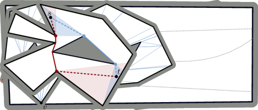
Figure 3: The augmented shortest path map of a vertex $v$. The shortest path map edges are solid, and the additional edges in the augmented shortest path map are dotted. Each region is bounded by three curves, of which at least two are line segments. Two regions and their apices are highlighted.

Augmented Shortest Path Maps.

In our approach, we build a data structure on the regions provided by the augmented shortest path maps of all vertices of $P$. The shortest path map of a point $p\in P$ is a partition of $P$ into maximal regions, such that for every point in a region $R$ the shortest path to $p$ traverses the same vertices of $P$ [30]. To obtain the augmented shortest path map $\mathit{SPM}(p)$, we connect each boundary vertex of $R$ with the apex $v_{R}$ of the region, i.e. the first vertex on the shortest path from any point in $R$ towards $p$. See Figure 3 for an example. All regions in $\mathit{SPM}(p)$ are “almost” triangles; they are bounded by three curves, two of which are line segments, and the remaining is either a line segment or a piece of a hyperbola. The (augmented) shortest path map has complexity $O(n)$ and can be constructed in $O(n\log n)$ time [30]. Let $\mathcal{T}$ be the multi-set of all augmented shortest path regions of all the vertices of $P$. As there are $n$ vertices in $P$, there are $O(n^{2})$ regions in $\mathcal{T}$.

Because we are only interested in shortest paths that contain at least one vertex, the shortest path between two points $s,t\in P$ consists of an edge from $s$ to some vertex $v$ of $P$ that is visible from $s$, a shortest path from $v$ to a vertex $u$ (possibly equal to $v$) that is visible from $t$, and an edge from $u$ to $t$. For two regions $S,T\in\mathcal{T}$ with $s\in S$ and $t\in T$, we define $f_{ST}(s,t)=||sv_{S}||+d(v_{S},v_{T})+||v_{T}t||$. The distance $d(s,t)$ between $s$ and $t$ is realised by this function when $v_{S}=v$ and $v_{T}=u$. As for any pair $S,T$ with $s\in S$ and $t\in T$ the function $f_{ST}(s,t)$ corresponds to the length of some path between $s$ and $t$ in $P$, we can obtain the shortest distance by taking the minimum over all of these functions. See Figure 4, and refer to Section 3 for the details. In other words, if we denote by $\mathcal{T}_{p}$ all regions that contain a point $p\in P$, we have

$$d(s,t)=\min\{f_{ST}(s,t):S\in\mathcal{T}_{s},\hskip 1.0ptT\in\mathcal{T}_{t}\}.$$

Figure 4: Two pairs of relevant regions in red and blue with the path whose length is $f_{ST}(s,t)$.

Lower Envelope.

Given two multi-sets $\mathcal{A},\mathcal{B}\subseteq\mathcal{T}$, we want to construct a data structure that we can efficiently query at any point $(s,t)$ with $s\in\bigcap\mathcal{A}$ and $t\in\bigcap\mathcal{B}$ to find $\min\{f_{ST}(s,t):S\in\mathcal{A},T\in\mathcal{B}\}$. We refer to this as a Lower Envelope data structure. We can construct such a data structure of size $O(\min\{|\mathcal{A}|,|\mathcal{B}|,n\}^{6+\varepsilon})$ with $O(\log(\min\{|\mathcal{A}|,|\mathcal{B}|,n\}))$ query time, or of size $O(\min\{|\mathcal{A}|,|\mathcal{B}|,n\}^{5+\varepsilon})$ with $O(\log^{2}(\min\{|\mathcal{A}|,|\mathcal{B}|,n\}))$ query time, as follows.

The functions $f_{ST}$ are four-variate algebraic functions of constant degree. Each such function gives rise to a surface in $\mathbb{R}^{5}$, which is the graph of the function $f$. Koltun [31] shows that the vertical decomposition of $m$ such surfaces in $\mathbb{R}^{5}$ has complexity $O(m^{6+\varepsilon})$, and can be stored in a data structure of size $O(m^{6+\varepsilon})$ so that we can query the value of the lower envelope, and thus $d(s,t)$, in $O(\log m)$ time. More recently, Agarwal et al. [2] showed that a collection of $m$ semialgebraic sets in $\mathbb{R}^{5}$ of constant complexity can be stored using $O(m^{5+\varepsilon})$ space such that vertical ray-shooting queries, and thus lower envelope queries, can be answered in $O(\log^{2}n)$ time.

We limit the number of functions $f_{ST}(s,t)$ by using an observation of Chiang and Mitchell [16]. They note that we do not need to consider all pairs $S\in\mathcal{A},T\in\mathcal{B}$, but only $\min\{|\mathcal{A}|,|\mathcal{B}|,n\}$ relevant pairs. Two regions form a relevant pair, if they belong to the same augmented shortest path map $\mathit{SPM}(v)$, of some vertex $v$. (To be specific, if $v$ is any vertex on the shortest path from $s$ to $t$, then the minimum is achieved for $S$ and $T$ in the shortest path map of $v$.) We thus obtain a Lower Envelope data structure by constructing the data structure of [2] or [31] on these $\min\{|\mathcal{A}|,|\mathcal{B}|,n\}$ functions.

Naively, to build a data structure that can answer shortest path queries for any pair of query points $s,t$, we would need to construct this data structure for all possible combinations of $\mathcal{T}_{s}$ and $\mathcal{T}_{t}$. The overlay of the $n$ augmented shortest path maps has worst-case complexity $\Omega(n^{4})$ [16], which implies that we would have to build $\Omega(n^{8})$ of the Lower Envelope data structures. Indeed, this results in an $O(n^{14+\varepsilon})$ size data structure, and is one of the approaches Chiang and Mitchell consider [16]. Next, we describe how we use cuttings to reduce the number of Lower Envelope data structures we construct.

Cutting Trees.

Now, we explain how to determine $\mathcal{T}_{s}$ more efficiently using cuttings and cutting trees. Suppose we have a set $\mathcal{A}$ of $N$ (not necessarily disjoint) triangles in the plane. A $1/r$-cutting $\Xi$ of $\mathcal{A}$ is then a subdivision of the plane into constant complexity cells, for example triangles, such that each cell in $\Xi$ is intersected by the boundaries of at most $N/r$ triangles in $\mathcal{A}$ [10]. There can thus still be many triangles that fully contain a cell, but only a limited number whose boundary intersects a cell. In our case, the regions in $\mathcal{T}$ are almost triangles, called Tarski cells [4]. See Section 4.1 for a detailed description of Tarski cells. As we explain in Section 4, we can always construct such a cutting with only $O(r^{2})$ cells for these types of regions efficiently.

Let $\Xi$ be a $1/r$-cutting of $\mathcal{T}$. For $s\in\Delta\in\Xi$ the regions $R\in\mathcal{T}$ that fully contain $\Delta$ also contain $s$. To be able to find the remaining regions in $\mathcal{T}_{s}$, we recursively build cuttings on the $N/r$ regions whose boundary intersects $\Delta$. This gives us a so-called cutting tree. By choosing $r$ appropriately, the cutting tree has constantly many levels. The set $\mathcal{T}_{s}$ is then the disjoint union of all regions obtained in a root-to-leaf path in the cutting tree. Note that using a constant number of point location queries it is possible to find all of the vertices on this path.

The Multi-Level Data Structure.

Our data structure, which we describe in detail in Sections 6 and 7, is essentially a multi-level cutting tree, as in [17]. See Figure 5 for an illustration. The first level is a cutting tree that is used to find the regions that contain $s$, as described before. For each cell $\Delta\in\Xi$ in a cutting $\Xi$, we construct another cutting tree to find the regions containing $t$. Let $\mathcal{A}$ be the set of regions fully containing $\Delta$ and $|\mathcal{A}|=k$, then the second-level cutting $\Xi_{\Delta}$ is built on the $O(kn)$ candidate relevant regions. See Figure 6. We process the regions intersected by a cell in $\Xi_{\Delta}$ recursively to obtain a cutting tree. Additionally, for each cell $\Delta^{\prime}\in\Xi_{\Delta}$, we construct the Lower Envelope data structure on the sets $\mathcal{A},\mathcal{B}$, where $\mathcal{B}$ is the set of regions that fully contain $\Delta^{\prime}$. This allows us to efficiently obtain $\min f_{ST}(s,t)$ for $S\in\mathcal{A}$ and $T\in\mathcal{B}$.

Figure 5: Overview of our data structure. The first level cutting tree (red) is built by recursively constructing a cutting $\Xi$ on the (orange) regions that intersect a cell $\Delta$ (purple). For each cell $\Delta$, we store a second level cutting tree (blue). For each cell $\Delta^{\prime}$ in $\Xi_{\Delta}$, we build a Lower Envelope data structure on all regions that fully contain $\Delta$ (dark red) and $\Delta^{\prime}$ (dark blue).

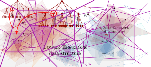
Figure 6: A sketch of the subproblem considered here, computing $\min_{S\in\mathcal{A},T\in\mathcal{T}}f_{ST}(s,t)$. We build a $1/r$-cutting $\Xi_{\Delta}$ (shown in purple) on the set of relevant regions in $\mathcal{T}$ (blue). The regions $\mathcal{T}_{t}\subseteq\mathcal{T}$ either fully contain the cell $\Delta^{\prime}\in\Xi_{\Delta}$ of the cutting that contains $t$ (dark blue), or their boundaries intersect $\Delta^{\prime}$ (light blue).

Queries.

To query our data structure with two points $s,t$, we first locate the cell $\Delta_{s}$ containing $s$ in the cutting $\Xi$ at the root. We compute $\min f_{ST}(s,t)$ for all regions $S$ that intersect $\Delta_{s}$, but do not fully contain $\Delta_{s}$, by recursively querying the child node corresponding to $\Delta_{s}$. To compute $\min f_{ST}(s,t)$ for all $S$ that fully contain $\Delta_{s}$, we query its associated data structure. To this end, we locate the cell $\Delta_{t}$ containing $t$ in $\Xi_{\Delta_{s}}$, and use its lower envelope structure to compute $\min f_{ST}(s,t)$ over all $S$ that fully contain $\Delta_{s}$ and all $T$ that fully contain $\Delta_{t}$. We recursively query the child corresponding to $\Delta_{t}$ to find $\min f_{ST}(s,t)$ over all $T$ that intersect $\Delta_{t}$.

Sketch of the Analysis.

By choosing $r$ as $n^{\delta}$ for some constant $\delta=O(\varepsilon)$, we can achieve that each cutting tree has only constant height. The total query time is thus $O(\log n)$, when using the Lower Envelope data structure by Koltun [31]. Next, we sketch the analysis to bound the space usage of the first-level cutting tree, under the assumption that a second-level cutting tree, including the Lower Envelope data structures, uses $O(n^{2}\min\{k,n\}^{6+\varepsilon})$ space (see Section 6).

To bound the space usage, we analyze the space used by the large levels, where the number of regions is greater than $n$, and the small levels of the tree separately, see Figure 7. There are only $O(n^{2})$ large nodes in the tree. For these $\min\{k,n\}=n$, so each stores a data structure of size $O(n^{8+\varepsilon})$. For the small nodes, the size of the second-level data structures decreases in each step, as $k$ becomes smaller than $n$. Therefore, the space of the root of a small subtree, which is $O(n^{8+\varepsilon})$, dominates the space of the other nodes in the subtree. As there are $O(n^{2})$ small root nodes, the resulting space usage is $O(n^{10+\varepsilon})$.

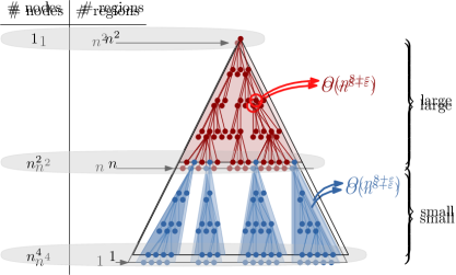
Figure 7: We analyze the large levels, built on $\geq n$ regions, and the small levels, built on $<n$ regions, separately. The total space usage is $O(n^{10+\varepsilon})$.

A space-time trade-off.

We can achieve a trade-off between the space usage and the query time by grouping the polygon vertices, see Section 8 for details. We group the vertices into $\ell$ groups, and construct our data structure on each set of $O(n^{2}/\ell)$ generated by a group. This results in a query time of $O(\ell\log^{2}n)$ and a space usage of $O(n^{9+\varepsilon}/\ell^{4+O(\varepsilon)})$ when we apply the vertical ray-shooting Lower Envelope data structure.

A data structure for $s$ or $t$ on the boundary.

In Section 9, we show how to adapt our data structure to the case where one (or both) of the query points, say $s$, is restricted to lie on the boundary of the domain. The main idea is to use the same overall approach as before, but consider a different set of regions for $s$ and $t$. The set of candidate regions for $s$ now consists of intervals formed by the intersection of the $\mathit{SPM}$ regions with the boundary of $P$. Instead of building a cutting tree on these regions, we build a segment tree, where nodes again store a cutting tree on the regions for $t$. As the functions $f_{ST}(s,t)$ are now only three-variate rather than four-variate, the resulting space usage is only $O(n^{6+\varepsilon})$.

When both query point are restricted to the boundary, the set of candidate regions for both $s$ and $t$ consists of intervals along $\partial P$. In this case, a node of the segment tree stores another segment tree on the regions for $t$. Because the functions $f_{ST}(s,t)$ are only bivariate, the space usage is reduced to $O(n^{4+\varepsilon})$.

2.1 Conclusion

Improving the space bound.

Both Lower Envelope data structures we use are actually more powerful than we require: one allows us to perform point location queries in the vertical decomposition of the entire arrangement, and the other allows us to perform vertical ray-shooting from any point in the arrangement. While we are only interested in lower envelope queries, i.e. vertical ray-shooting from a single plane. The (projected) lower envelope of $m$ four-variate functions has a complexity of only $O(m^{4+\varepsilon})$ [36]. However, it is unclear if we can store this lower envelope in a data structure of size $O(m^{4+\varepsilon})$ while retaining the $O(\log m)$ query time. This would immediately reduce the space of our data structure to $O(n^{8+\varepsilon})$.

3 Decomposing the distance computation

As described in Section 2, we assume that there is at least one vertex on the shortest path between two query points. We will decompose the distance computation using the regions from the augmented shortest path maps of all vertices. Let $\mathit{SPM}^{\prime}(p)$ be the shortest path map of source point $p$ in $P$, i.e. a partition of $P$ into maximal closed regions such that for every point in such a region $R$ the shortest path to $p$ visits the same sequence of polygon vertices [30]. Let $v_{R}$ be the first vertex on the shortest path from any point in $R$ towards $p$. We refer to $v_{R}$ as the apex of region $R$. We “triangulate” every region $R$ of $\mathit{SPM}^{\prime}(p)$ by connecting the boundary vertices of $R$ with the apex $v_{R}$. The resulting subdivision of $P$ is the augmented shortest path map $\mathit{SPM}(p)$ of $P$ with respect to source point $p$. All regions in $\mathit{SPM}(p)$ consist of at most three curves, two of which are line segments, and the remaining edge is either a line segment or a piece of a hyperbola, see Figure 3. The (augmented) shortest path map has complexity $O(n)$ [30].

Consider the augmented shortest path maps for all vertices of $P$, and let $\mathcal{T}$ denote the multi-set of all such regions. Hence, $\mathcal{T}$ consists of $O(n^{2})$ regions. We associate with each region in $\mathcal{T}$ the vertex of $P$ that generated the region. Let $\mathcal{T}_{s}\subset\mathcal{T}$ be the subset of regions that contain a point $s\in P$.

For a pair $S,T\in\mathcal{T}\times\mathcal{T}$ we define $f_{ST}(s,t)=\|sv_{S}\|+d(v_{S},v_{T})+\|v_{T}t\|$ for $s\in S$ and $t\in T$, see Figure 4. Observe that $f_{ST}$ is essentially a 4-variate algebraic function of constant complexity (since $d(v_{S},v_{T})$ is constant with respect to $s$ and $t$). For a pair of points $s,t$ that cannot see each other we then have that

$$d(s,t)=\min_{S\in\mathcal{T}_{s},T\in\mathcal{T}_{t}}\|sv_{S}\|+d(v_{S},v_{T})+\|v_{T}t\|=\min\{f_{ST}(s,t):S\in\mathcal{T}_{s},\hskip 1.0ptT\in\mathcal{T}_{t}\}.$$ (1)

Note that whenever either of the two query points lies on a polygon vertex, we can directly answer the query by considering the shortest path map of that vertex.

Relevant region-pairs.

We say that a pair of regions $(S,T)$ is relevant if and only if they appear in a single augmented shortest path map $\mathit{SPM}(v)$ for some vertex $v$. Let $\mathit{Rel}(\chi)=\{(S,T)\mid(S,T)\in\chi\land(S,T)\text{ is relevant }\}$ denote the subset of relevant pairs of regions from a set of pairs $\chi$. Chiang and Mitchell [16] observed that $d(s,t)$ is defined by a pair of relevant regions. Let $\mathcal{L}^{\chi}(s,t)=\min\{f_{ST}(s,t):(S,T)\in\mathit{Rel}(\chi)\}$. We thus have:

[Chiang and Mitchell [16]] There exists a pair $(S,T)\in\mathcal{T}_{s}\times\mathcal{T}_{t}$ such that: (i) the pair $(S,T)$ is relevant, and (ii) $d(s,t)=f_{ST}(s,t)$. Hence,

$$d(s,t)=\mathcal{L}^{\mathcal{T}_{s}\times\mathcal{T}_{t}}(s,t)=\min\{f_{ST}(s,t):(S,T)\in\mathit{Rel}(\mathcal{T}_{s}\times\mathcal{T}_{t})\}.$$

Proof 3.1.

Let $\pi(s,t)$ be an optimal path, and let $v$ be the first vertex of $\pi(s,t)$. Pick $S$ and $T$ as regions in $\mathit{SPM}(v)$ containing $s$ and $t$, respectively.

Note that in this proof we can choose $S$ as any region in $\mathit{SPM}(v)$ that contains $s$. Thus, if $s$ lies on the boundary of multiple regions, any of these regions will achieve the optimal distance. This implies that the set $\mathcal{T}_{s}$ can be limited to only one regions from each shortest path map, so $|\mathcal{T}_{s}|=O(n)$, and similarly $|\mathcal{T}_{t}|=O(n)$.

Lemma 3.2.

Let $\mathcal{A}\subseteq\mathcal{T}_{s}$, $\mathcal{B}\subseteq\mathcal{T}_{t}$ be two sets of regions. The set $\mathit{Rel}(\mathcal{A}\times\mathcal{B})$ contains at most $m=O(\min\{|\mathcal{A}|,|\mathcal{B}|\})\leq O(n)$ pairs of regions.

Proof 3.3.

As stated before, $\mathcal{T}_{s}$, and thus $\mathcal{A}$, contains at most $O(n)$ regions. The same applies for $\mathcal{T}_{t}$ and $\mathcal{B}$, hence $|\mathcal{A}|$ and $|\mathcal{B}|$ are $O(n)$.

Assume without loss of generality that $|\mathcal{A}|\leq|\mathcal{B}|$. What remains to show is that $\mathit{Rel}(\mathcal{A}\times\mathcal{B})$ contains at most $O(|\mathcal{A}|)$ regions. We charge every pair $(S,T)\in\mathit{Rel}(\mathcal{A}\times\mathcal{B})$ to $S$, and argue that each region $S$ can be charged at most a constant number of times. Let $v$ be the vertex associated with $S$, i.e. the vertex that generated the region. Consider all regions $T_{1},..,T_{z}$ such that $(S,T_{i})\in\mathit{Rel}(\mathcal{A}\times\mathcal{B})$. All of these regions must appear in $\mathit{SPM}(v)$ and contain $t$. There are at most $O(1)$ such regions. Hence, it follows that each region $S$ is charged at most $O(1)$ times, and there are thus at most $O(|\mathcal{A}|)$ pairs of regions in $\mathit{Rel}(\mathcal{A}\times\mathcal{B})$.

Furthermore, we observe that computing $\mathcal{L}^{\mathcal{A}\times\mathcal{B}}(s,t)$ is decomposable:

Lemma 3.4.

Let $\mathcal{A},\mathcal{B}\subseteq\mathcal{T}$ be sets of regions, let $\mathcal{A}_{1},..,\mathcal{A}_{k}$ be a partition of $\mathcal{A}$, and let $\mathcal{B}_{1},..,\mathcal{B}_{\ell}$ be a partition of $\mathcal{B}$. We have that

$$\mathcal{L}^{\mathcal{A}\times\mathcal{B}}(s,t)=\min\{\mathcal{L}^{\mathcal{A}_{i}\times\mathcal{B}_{j}}(s,t):i\in\{1,..,k\},j\in\{1,..,\ell\}\}.$$

Proof 3.5.

Recall that $\mathcal{L}^{\mathcal{A}\times\mathcal{B}}(s,t)=\min\{f_{ST}(s,t):(S,T)\in\mathit{Rel}(\mathcal{A}\times\mathcal{B})\}$. Since computing the minimum is decomposable, all that we have to argue is that $\mathit{Rel}(\mathcal{A}\times\mathcal{B})=\bigcup_{i\in\{1,..,k\},j\in\{1,..,\ell\}}\mathit{Rel}(\mathcal{A}_{i}\times\mathcal{A}_{j})$. By definition of $\mathit{Rel}$ we have

$$\mathit{Rel}((\mathcal{X}\cup\mathcal{Y})\times\mathcal{Z}) =\{(S,T)\mid(S,T)\in(\mathcal{X}\cup\mathcal{Y})\times\mathcal{Z}\land(S,T)\text{ is relevant }\}$$

$$=\{(S,T)\mid(S,T)\in\mathcal{X}\times\mathcal{Z}\land(S,T)\text{ is relevant }\}$$

$$\cup\{(S,T)\mid(S,T)\in\mathcal{Y}\times\mathcal{Z}\land(S,T)\text{ is relevant }\}$$

$$=\mathit{Rel}(\mathcal{X}\times\mathcal{Z})\cup\mathit{Rel}(\mathcal{Y}\times\mathcal{Z}),$$

and symmetrically $\mathit{Rel}(\mathcal{X}\times(\mathcal{Y}\cup\mathcal{Z}))=\mathit{Rel}(\mathcal{X}\times\mathcal{Y})\cup\mathit{Rel}(\mathcal{X}\times\mathcal{Z})$. The lemma now follows from repeated application of these equalities.

By Observation 3 we have that $d(s,t)=\mathcal{L}^{\mathcal{T}_{s}\times\mathcal{T}_{t}}(s,t)$. Applying Lemma 3.4 to $\mathcal{T}_{s}$ and $\mathcal{T}_{t}$, thus tells us that we can compute $d(s,t)$ using a divide and conquer approach. We will use cuttings to do so.

4 Cuttings

In this section we first introduce Tarski cells. We then define a $1/r$-cutting on a set of Tarski cells, and prove that such a cutting exists and can be computed efficiently.

4.1 Tarski Cells

A Tarski cell is a region of $\mathbb{R}^{2}$ bounded by a constant number of semi-algebraic curves of constant degree [4]. Observe that the regions generated by the shortest path maps are thus Tarski cells. A pseudo trapezoid is a Tarski cell that is bounded by at most two vertical line segments and at most two $x$-monotone curves. Observe that a pseudo trapezoid itself is thus also $x$-monotone. Given a set $\mathcal{T}$ of $N$ of Tarski cells, let $\mathcal{A}(\mathcal{T})$ denote their arrangement, and let $\mathcal{VD}(\mathcal{T})$ denote the vertical decomposition of $\mathcal{A}(\mathcal{T})$ into pseudo trapezoids. It is well known that both $\mathcal{A}(\mathcal{T})$ and $\mathcal{VD}(\mathcal{T})$ have complexity $O(N^{2})$ (as any pair of curves intersects at most a constant number of times, and each curve has at most a constant number of points at which it is tangent to a vertical line).

4.2 Cuttings on Tarski Cells

Let $\mathcal{T}$ be a set of $N$ regions, each a Tarski cell, and let $r\in\{1,..,N\}$ be a parameter. Before we can introduce cuttings, we need to define conflict lists. We say, a region $T\in\mathcal{T}$ conflicts with a cell $\nabla\subseteq\mathbb{R}^{2}$ if the boundary of $T$ intersects the interior of $\nabla$. The conflict list $\mathcal{C}_{\nabla}$ of $\nabla$ (with respect to $\mathcal{T}$) is the set of all region $T\in\mathcal{T}$ that conflict with it.

A $1/r$-cutting $\Xi$ of $\mathcal{T}$ is a partition of $\mathbb{R}^{2}$ into Tarski cells, each of which is intersected by the boundaries of at most $N/r$ regions in $\mathcal{T}$, i.e. has a conflict list of size at most $N/r$ [10]. The following two Lemmas summarize that such cuttings exist, and can be computed efficiently.

Lemma 4.1.

Let $\mathcal{T}$ be a set of $N$ Tarski cells, and let $c$ be a constant. For a random subset $\mathcal{R}\subseteq\mathcal{T}$ of size $r$, we can compute $\mathcal{VD}(\mathcal{R})$, and all conflict lists in expected $O(Nr)$ time. Furthermore, we have that

$$\mathbb{E}\left[\sum_{\nabla\in\mathcal{VD}(\mathcal{R})}|\mathcal{C}_{\nabla}|^{c}\right]=O(r^{2}(N/r)^{c}).$$

Proof 4.2.

The bound on the expected value of the quantity $W^{c}_{i}=\sum_{\nabla\in\mathcal{VD}(\mathcal{R})}|\mathcal{C}_{\nabla}|^{c}$ follows from a Clarkson-Shor type sampling argument [18]. Therefore, we can compute $\mathcal{VD}(\mathcal{R})$ and its conflict lists by running the first $r$ rounds of a randomized incremental construction algorithm. For completeness, we include the detailed argument here. Our presentation is based on that of Har-Peled [28].

Algorithm.

We build the vertical decomposition $\mathcal{VD}(\mathcal{R})$ by running a randomized incremental construction algorithm [28] to construct $\mathcal{VD}(\mathcal{T})$ for only $r$ rounds. Let $T_{1},..,T_{r}$ denote the regions in the random order, and let $\mathcal{R}_{i}=\{T_{1},..,T_{i}\}$ be the subset containing the first $i$ regions. So $\mathcal{R}=\mathcal{R}_{r}$. We maintain a bipartite conflict graph during the algorithm; the sets of vertices are the pseudo-trapezoids in $\mathcal{VD}(\mathcal{R}_{i})$ and the not-yet inserted regions from $\mathcal{T}\setminus\mathcal{R}_{i}$. The conflict graph has an edge $(\nabla,T)$ if and only if $T\in\mathcal{C}^{\mathcal{T}}_{\nabla}$. Using this conflict graph, it straightforward to insert a new region $T_{i}$ into $\mathcal{VD}(\mathcal{R}_{i-1})$; the conflict graph tells us exactly which pseudo trapezoids from $\mathcal{VD}(\mathcal{R}_{i-1})$ should be deleted; each of which is replaced by $O(1)$ new pseudo-trapezoids.

Let $E_{i}$ be the total number of newly created edges in the conflict graph in step $i$ (i.e. the total number of new entries in the conflict lists), and let $W_{i}=W^{1}_{i}$ denote the total size of all conflicts of the pseudo-trapezoids in $\mathcal{VD}(\mathcal{R}_{i})$. The time required by step $i$ of the algorithm is linear in $E_{i}$. We will argue that $\mathbb{E}[E_{i}]=O(N)$, and thus the total expected running time is $O(Nr)$.

Analyzing $\mathbb{E}[E_{i}]$.

For a particular pseudo trapezoid $\nabla\in\mathcal{VD}(\mathcal{R}_{i})$, the probability that $\nabla$ was created by inserting region $T_{i}$ is at most $4/i$ (since $T_{i}$ must contribute to one of the four boundaries of $\nabla$). Therefore, the expected size of $E_{i}$, conditioned on the fact that the vertical decomposition after $i$ rounds is $\mathcal{VD}(\mathcal{R}_{i})$, is $\mathbb{E}[E_{i}\mid\mathcal{VD}(\mathcal{R}_{i})]=O(\mathbb{E}[W_{i}]/i)$. Using the law of total expectation, it then follows that $\mathbb{E}[E_{i}]=\mathbb{E}[\mathbb{E}[W_{i}\mid\mathcal{VD}(\mathcal{R}_{i})]]=O(\mathbb{E}[W_{i}]/i)$. As we argue next, we have that $\mathbb{E}[W^{c}_{i}]=O((N/i)^{c}i^{2})$, and therefore $\mathbb{E}[W_{i}]=\mathbb{E}[W^{1}_{i}]=O(Ni)$. In turn, this gives us $\mathbb{E}[E_{i}]=O(Ni/i)=O(N)$ as claimed.

Analyzing $\mathbb{E}[W^{c}_{i}]$.

Let $M_{i,\geq k}$ denote the set of pseudo trapezoids from $\mathcal{VD}(\mathcal{R}_{i})$ whose conflict list has size at least $k$. So note that $M_{i,\geq 0}$ is simply the total number of trapezoids in $\mathcal{VD}(\mathcal{R}_{i})$.

The main idea is that the probability that a pseudo trapezoid from $\mathcal{VD}(\mathcal{R}_{i})$ has a conflict list that is at least $t$ times the average size $N/i$ decreases exponentially with $t$. In particular, since every such pseudo trapezoid $\nabla$ is defined by at most $d=O(1)$ regions from $\mathcal{T}$, and conflicts with more than $tN/i$ regions, the probability of it appearing in $\mathcal{VD}(\mathcal{R}_{i})$ is at most ${n-d-t(N/i)\choose i}/{n\choose i}\approx(1-(n/i))^{t(n/i)}(n/i)^{d}$. This is roughly $1/e^{t}$ times the probability that a pseudo trapezoid with a conflict list of size $n/i$ appears in $\mathcal{VD}(\mathcal{R}_{i})$ (which, analogously, is roughly $(1-(n/i))^{(n/i)}(n/i)^{d}$). This then allows us to express the expected number of such “heavy” pseudo trapezoids by the expected number of “average” pseudo trapezoids. More precisely, we have that $\mathbb{E}[M_{i,\geq tN/i}]=O\left(\mathbb{E}[M_{i,\geq 0}]\cdot t^{d}\cdot\textrm{tiny}(t)\right)$, where $\textrm{tiny}(t)=1/e^{(t/2)}$ [28, Lemma 8.7]. Har-Peled refers to this as the exponential decay Lemma.

We then get

$$\mathbb{E}\left[\sum_{\nabla\in\mathcal{VD}(\mathcal{R}_{i})}|C^{\mathcal{T}}_{\nabla}|^{c}\right] \leq\mathbb{E}\left[\sum_{t\geq 1}\left(t\frac{N}{i}\right)^{c}(M_{i,\geq(t-1)(N/i)}-M_{i,\geq t(N/i)})\right]$$

$$\leq\mathbb{E}\left[\left(\frac{N}{i}\right)^{c}\sum_{t\geq 0}(t+1)^{c}M_{i,\geq t(N/i)}\right]$$

$$\leq\left(\frac{N}{i}\right)^{c}\sum_{t\geq 0}(t+1)^{c}\leavevmode\nobreak\ \mathbb{E}\left[M_{i,\geq t(N/i)}\right]\text{ \{exponential decay lemma\} }$$

$$\leq\left(\frac{N}{i}\right)^{c}\sum_{t\geq 0}(t+1)^{c}O\left(t^{d}\,\textrm{tiny}(t)\leavevmode\nobreak\ \mathbb{E}\left[M_{i,\geq 0}\right]\right)$$

$$\leq O\left(\left(\frac{N}{i}\right)^{c}\leavevmode\nobreak\ \mathbb{E}\left[M_{i,\geq 0}\right]\sum_{t\geq 0}(t+1)^{c+d}\,\textrm{tiny}(t)\right)$$

$$=O\left(\left(\frac{N}{i}\right)^{c}\mathbb{E}\left[M_{i,\geq 0}\right]\right)=O\left(\left(\frac{N}{i}\right)^{c}i^{2}\right).$$

So in particular, for $i=r$, we obtain $\mathbb{E}[W^{c}_{r}]=O(r^{2}(N/r)^{c})$ as claimed. This completes the proof.

Lemma 4.3.

Let $\mathcal{T}$ be a set of $N$ Tarski cells, and $r\in\{1,..,N\}$ a parameter. An $1/r$-cutting $\Xi$ of $\mathcal{T}$ of size $O(r^{2})$, together with its conflict lists, can be computed in expected $O(Nr)$ time.

Proof 4.4.

The fact that $\Xi$ exists, and has size $O(r^{2})$ follows by combining the approach of Agarwal and Matoušek [4] with the results of de Berg and Schwarzkopf [20]. In particular, Agarwal and Matoušek show that a $1/r$-cutting of size $O(r^{2}\log^{2}r)$ exists (essentially the vertical decomposition of a random sample of size $O(r\log r)$ will likely be a $1/r$-cutting). Plugging this into the framework of de Berg and Schwartzkopf gives us that $1/r$-cutting of size $O(r^{2})$ exists. We can use the algorithm in Lemma 4.1 to construct the vertical decomposition as needed by the Agarwal and Matoušek algorithm, as well as to implement the framework of de Berg and Schwartzkopf.

For completeness, we include the full argument here. Let $\mathcal{E}$ denote the family of Tarski cells in $\mathbb{R}^{2}$, and observe that $\mathcal{T}\subset\mathcal{E}$. The range space $(\mathcal{E},\{\mathcal{C}_{\Delta}\mid\Delta\in\mathcal{E}\})$ has constant VC-dimension [4]. Furthermore, for some subset $\mathcal{T}^{\prime}\subset\mathcal{E}$ of size $m$, the vertical decomposition $\mathcal{VD}(\mathcal{T}^{\prime})$ of the arrangement of $\mathcal{T}^{\prime}$ has size $O(m^{2})$. Therefore, by Lemma 3.1 of Agarwal and Matoušek [4], the vertical decomposition $\mathcal{VD}(\mathcal{N})$ of a $1/r$-net $\mathcal{N}$ of $\mathcal{T}$ of size $m=O(r\log r)$ is an $1/r$-cutting of $\mathcal{T}$ of size $O(m^{2})=O(r^{2}\log^{2}r)$. (Recall that $\mathcal{N}$ is an $1/r$ net for $\mathcal{T}$ if for every range $\mathcal{C}_{\Delta}$ of size at least $|\mathcal{T}|/r$ contains at least one region from $\mathcal{N}$.)

We can compute such an $1/r$-net, together with its conflict lists, in expected $O(Nm)=O(Nr\log r)$ time. Indeed, taking a random sample $\mathcal{N}$ of size $O(r\log r)$ is expected to be a $1/r$-net for $\mathcal{T}$ with constant probability. So, we can simply construct $\mathcal{VD}(\mathcal{N})$ and its conflict lists using Lemma 4.1. If $\mathcal{N}$ is not a $1/r$-net (i.e. the size of the conflict lists grows beyond size $O(Nr\log r)$), we discard the results, and start fresh with a new random sample. The expected number of retries is constant, and thus the expected time to construct a $1/r$-cutting is $O(Nr\log r)$.

We now use the results of de Berg and Schwarzkopf to obtain a cutting of size $O(r^{2})$ [20]. Let $\mathcal{R}\subseteq\mathcal{T}$ be an arbitrary subset of regions from $\mathcal{T}$. The vertical decomposition has the role of what de Berg and Schwarzkopf call a “canonical triangulation”. In particular, observe that we have the following properties:

C1

Each pseudo-trapezoid $\Delta\in\mathcal{VD}(\mathcal{R})$ is defined by a constant size defining set $\mathcal{D}\subseteq\mathcal{R}$. More precisely, we need that $\Delta$ is a pseudo-trapezoid in $\mathcal{VD}(\mathcal{D})$.

C2

For each pseudo-trapezoid $\Delta\in\mathcal{VD}(\mathcal{R})$, the pseudo-trapezoid also appears in $\mathcal{VD}(\mathcal{T})$ if and only if the conflict list $\mathcal{C}_{\Delta}$ with respect to $\mathcal{T}$ is empty.

C3

For a parameter $t\geq 1$, there exists a $1/t$-cutting of $\mathcal{R}$ of size $O(t^{2}\log^{2}t)=O(t^{3})$ (as we argued above).

Therefore, we can apply the results of de Berg and Schwarzkopf [20]. In particular, their Lemma 1 gives us that exists an $1/r$-cutting of $\mathcal{T}$ of size $O(r^{2})$ (since the expected number of pseudo-trapezoids in $\mathcal{VD}(\mathcal{R})$ in a random sample $\mathcal{R}\subseteq\mathcal{T}$ of size $r$ is $O(r^{2})$.

All that remains is to argue that we can construct such a cutting in expected $O(nr)$ time. We follow a similar presentation as Har-Peled [28]. We take a random sample $\mathcal{R}$ of size $r$, and compute the vertical decomposition $\mathcal{VD}(\mathcal{R})$ and its conflict lists using Lemma 4.1. For each pseudo-trapezoid $\nabla\in\mathcal{VD}(\mathcal{R})$ whose conflict list is larger than $CN/r$, for some constant $C$, we compute a $1/t_{\nabla}$-cutting of $|\mathcal{C}_{\nabla}|$, for $t_{\nabla}=|\mathcal{C}_{\nabla}|r/N$ and clip it to $\nabla$. We use the approach based on $1/t_{\nabla}$-nets for these cuttings. Hence, the expected time to construct all of them is

$$\sum_{\nabla\in\mathcal{VD}(\mathcal{R})}O(|\mathcal{C}_{\nabla}|t_{\nabla}\log t_{\nabla}) =\sum_{\nabla\in\mathcal{VD}(\mathcal{R})}O(|\mathcal{C}_{\nabla}|t_{\nabla}^{2})=\sum_{\nabla\in\mathcal{VD}(\mathcal{R})}O(|\mathcal{C}_{\nabla}|^{3}r^{2}/N^{2})$$

$$=O(r^{2}/N^{2})\sum_{\nabla\in\mathcal{VD}(\mathcal{R})}|\mathcal{C}_{\nabla}|^{3}.$$

By Lemma 4.1 the total expected time is therefore $O((r^{2}/N^{2})r^{2}(N/r)^{3})=O(Nr)$. Clipping the resulting cells can be done in the same time. By Lemma 1 of Berg and Schwarzkopf [20] the result is a $1/r$-cutting.

5 A data structure for when $\mathcal{T}_{s}$ and $\mathcal{T}_{t}$ are given

In this section, we consider the subproblem of finding the minimum distance over a fixed set of regions. Let $\mathcal{A},\mathcal{B}\subseteq\mathcal{T}$ be two sets of regions, and let $m=\min\{|\mathcal{A}|,|\mathcal{B}|,n\}$. We construct a data structure on the regions in $\mathcal{A}$ and $\mathcal{B}$ such that we can compute the lower envelope $\mathcal{L}^{\mathcal{A}\times\mathcal{B}}(s,t)$ for any query points $s\in\bigcap\mathcal{A}$ and $t\in\bigcap\mathcal{B}$ efficiently. We call such a data structure a Lower Envelope data structure.

Observe that all regions in $\mathcal{A}$ overlap in some point $a$, and all regions in $\mathcal{B}$ overlap in some point $b$. So $\mathcal{A}\subseteq\mathcal{T}_{a}$, and $\mathcal{B}\subseteq\mathcal{T}_{b}$. It then follows from Lemma 3.2 that $\mathit{Rel}(\mathcal{A}\times\mathcal{B})$ has size $O(m)=O(\min\{|\mathcal{A}|,|\mathcal{B}|,n\})$. The functions $f_{ST}$, for $(S,T)\in\mathit{Rel}(\mathcal{A}\times\mathcal{B})$ are four-variate, and have constant algebraic degree. The Lower Envelope data structure thus has to be constructed on only $O(m)$ four-variate functions. Next, we consider two Lower Envelope data structures that can be built on a given set of functions $f_{ST}$.

Lemma 5.1.

For any constant $\varepsilon>0$, we can construct a Lower Envelope data structure of size $O(m^{6+\varepsilon})$ in $O(m^{6+\varepsilon})$ expected time, that can answer queries in $O(\log m)$ time.

Proof 5.2.

One way obtain efficient queries of $\mathcal{L}(s,t)$ is by storing the vertical decomposition of (the graphs of) the functions $f_{ST}$ for all $(S,T)\in\mathit{Rel}(\mathcal{A}\times\mathcal{B})$. Koltun [31] shows that the vertical decomposition of $m$ surfaces in $\mathbb{R}^{d}$, each described by an algebraic function of constant degree, has complexity $O(m^{2d-4+\varepsilon})$, and can be stored in a data structure of size $O(m^{2d-4+\varepsilon})$. This data structure can also be constructed in $O(m^{2d-4+\varepsilon})$ expected time, and we can query the value of the lower envelope by a point location query in $O(\log m)$ time [11].

Since our functions are four-variate, we have $d=5$, and thus we get an $O(m^{6+\varepsilon})$ size data structure that answers queries in $O(\log m)$ time.

Lemma 5.3.

For any constant $\varepsilon>0$, we can construct a Lower Envelope data structure of size $O(m^{5+\varepsilon})$ in $O(m^{5+\varepsilon})$ expected time, that can answer queries in $O(\log^{2}m)$ time.

Proof 5.4.

An alternative way to query $\mathcal{L}(s,t)$ is to perform a vertical ray-shooting query. Agarwal et al. [2] show that a collection of $m$ semialgebraic sets in $\mathbb{R}^{d}$, each of constant complexity, can be stored in a data structure of size $O(m^{d+\varepsilon})$, for any constant $\varepsilon>0$, that allows for vertical ray-shooting queries in $O(\log^{2}m)$ time. The data structure can also be constructed in $O(m^{d+\varepsilon})$ expected time. As the (graphs of) our functions $f_{ST}$ are semialgebraic sets in $\mathbb{R}^{5}$, this gives an $O(m^{5+\varepsilon})$ size data structure that can answer queries in $O(\log^{2}m)$ time.

6 A data structure for when $\mathcal{T}_{s}$ is given

Let $\mathcal{A},\mathcal{B}\subseteq\mathcal{T}$ be two subsets of regions with $|\mathcal{A}|=k$, and $|\mathcal{B}|=M_{0}$. We develop a data structure to store $\mathcal{L}^{\mathcal{A}\times\mathcal{B}}$ that can efficiently compute $\mathcal{L}^{\mathcal{A}\times\mathcal{B}}(s,t)$, provided that $s\in\bigcap\mathcal{A}$. As before, this implies that $\mathcal{T}_{s}\supseteq\mathcal{A}$, and thus $k=O(n)$. Moreover, if $\mathcal{A}=\mathcal{T}_{s}$ and $\mathcal{B}=\mathcal{T}$ this thus allows us to compute $d(s,t)$ for any $t\in P$. As there are at most $nk$ relevant regions for $t$, we can assume that $M_{0}\leq nk$. We can compute these relevant regions, and store for each region in $\mathcal{A}$ a bidirectional pointer to its relevant region in $\mathcal{B}$, in $O(n^{2}\log n)$ time by sorting the regions and performing a linear search. We formulate our result with respect to any Lower Envelope data structure that uses $S(m)$ space and expected preprocessing time on $m$ functions, and has query time $Q(m)$, where $S(m)$ is of the form $Cm^{a}$ for some constants $C>0$ and $a\geq 3$, and $Q(m)$ is non-decreasing. In this section, we prove the following lemma.

Lemma 6.1.

For any constant $\varepsilon>0$, there is a data structure of size $O(n^{2+\varepsilon}S(k))$, so that for any query points $s,t$ for which $s\in\bigcap\mathcal{A}$ we can compute $\mathcal{L}^{\mathcal{A}\times\mathcal{B}}(s,t)$ in $O(\log n+Q(k))$ time. Building the data structure takes $O(n^{2+\varepsilon}S(k))$ expected time.

Note that if we are somehow given $\mathcal{A}=\mathcal{T}_{s}$, and have $\mathcal{B}=\mathcal{T}$ then $k=n$, and thus we get an $O(n^{2+\varepsilon}S(n))$ size data structure that can compute $d(s,t)$ in $O(\log n+Q(n))$ time.

Our data structure is essentially a cutting-tree [17] in which each node stores an associated Lower Envelope data structure (Section 5). In detail, let $r\in\{2,..,M_{0}\}$ be a parameter to be determined later. We build a $1/r$-cutting $\Xi^{\prime}$ of $\mathcal{B}$ using the algorithm from Lemma 4.3. Furthermore, we preprocess $\Xi^{\prime}$ for point location queries [23]. For each cell $\Delta\in\Xi^{\prime}$, the subset $\mathcal{B}_{\Delta}$ of regions of $\mathcal{B}$ that contain $\Delta$ have an apex visible from any point within $\Delta$. (Since all points in a region $T$ see its apex $v_{T}$, i.e. the line segment to $v_{T}$ does not intersect $\delta P$, and $\Delta$ is contained in $T$.) Hence, we store a Lower Envelope data structure on the pair of sets $(\mathcal{A},\mathcal{B}_{\Delta})$ for each cell $\Delta$. We now recursively process the set $\mathcal{C}_{\Delta}$ of regions whose boundary intersects $\Delta$.

All that remains is to describe how to choose the parameter $r$ that we use to build the cuttings. Let $c$ be the constant so that the number of cells in a $1/r$-cutting on $\mathcal{B}$ has at most $cr^{2}$ cells. The idea is to pick $r=\max\{n^{\delta},2,2c^{1/(a-2)}\}$, for some fixed $\delta\in(0,1)$ to be specified later.

Space usage.

Let $M$ be the number of remaining regions from $\mathcal{B}$ (initially $M=M_{0}$). Storing the cutting $\Xi_{\Delta}$, and its point location structure takes $O(r^{2})$ space [23]. Moreover, for each of the $O(r^{2})$ cells, we store a Lower Envelope data structure of size $S(\min(k,M))$. There are only $M/r$ regions whose boundary intersects a cell of the cutting on which we recurse. The space usage of the data structure is thus given by the following recurrence:

$$\mathcal{S}(M)=\begin{cases}cr^{2}\mathcal{S}(M/r)+O\left(r^{2}\cdot S(\min\{k,M\})\right)&\text{if }M>1\\ O(1)&\text{if }M=1.\end{cases}$$

After $i$ levels of recursion, this gives $O(r^{2i})=O(n^{2\delta i})$ subproblems of size at most $M_{0}/r^{i}\leq nk/n^{\delta i}=n^{1-\delta i}k$. It follows that at level $\frac{1}{\delta}$, we have $O(n^{2})$ subproblems of size $O(k)$. Next, we analyze the space usage by the higher levels, where $i\leq\frac{1}{\delta}$, and lower levels, where $i>\frac{1}{\delta}$, separately. Note that for the higher levels, we have $\min\{k,M\}=k$, and for the lower levels $\min\{k,M\}=M$. There are only $\frac{1}{\delta}=O(1)$ higher levels.

In the higher levels of our data structure, the $O(r^{2i})$ associated Lower Envelope data structures at level $i\leq\frac{1}{\delta}$, take $O(r^{2i}\cdot r^{2}\cdot S(k))=O(n^{2+\varepsilon}S(k))$ space, by setting $\delta=\varepsilon/2$. Since there are only $O(1)$ higher levels, the total space usage of these levels is $O(n^{2+\varepsilon}S(k))$ as well.

In the lower levels of our data structure, we are left with $O(n^{2})$ “small” subproblems at level $i=\frac{1}{\delta}$. In the following we argue that such a “small” subproblem uses only $O(r^{2}S(k))$ space, and therefore the lower levels also use only $O(n^{2+\varepsilon}S(k))$ space in total.

For each such “small” subproblem, we have a $1/r$-cutting on $M\leq k$ regions that consists of at most $cr^{2}$ cells. Since $M\leq k$, the recurrence simplifies to

$$\mathcal{S}^{\prime}(M)=\begin{cases}cr^{2}\mathcal{S}^{\prime}(M/r)+dr^{2}S(M)&\text{if }M>1\\ e&\text{if }M=1,\end{cases}$$

where $c,d$, and $e$ are positive constants.

Lemma 6.2.

Let $c,d,e,\varepsilon>0$ be constants and $r>\max\{2,2c^{1/4}\}$. The recurrence $\mathcal{S}^{\prime}(M)$ solves to $O(r^{2}S(M))$.

Proof 6.3.

We prove by induction on $M$ that $\mathcal{S}(M)\leq Dr^{2}M^{6+\varepsilon}$, for constant $D\geq\max\{2d,e\}$. The base case $M=1$ is trivial. Using the induction hypothesis we then have that

$$cr^{2}\mathcal{S}(M/r)+dr^{2}S(M)\leq cr^{2}\left(Dr^{2}S\left(\frac{M}{r}\right)\right)+dr^{2}S(M)=cDr^{4}S\left(\frac{M}{r}\right)+dr^{2}S(M)$$

Using some basic calculus we then find that:

$$cDr^{4}S\left(\frac{M}{r}\right)+dr^{2}S(M) =cDr^{4}\frac{M^{a}}{r^{a}}+dr^{2}M^{a}$$

$$=r^{2}M^{a}\left(\frac{cD}{r^{a-2}}+d\right)$$

$$\leq r^{2}M^{a}\left(\frac{cD}{(2c^{1/(a-2)})^{a-2}}+d\right)$$

$$\leq r^{2}M^{a}\left(\frac{D}{2}+d\right)$$

$$\leq Dr^{2}M^{a}=Dr^{2}S(M)$$

Here, we used that $a\geq 3$, $r>2c^{1/(a-2)}$, and $D\geq 2d$. This completes the proof.

Analyzing the preprocessing time.

By Lemma 4.3 we can construct a $1/r$-cutting on $\mathcal{B}$, together with the conflict lists, in $O(rM)$ expected time. Since the cutting has size $O(r^{2})$, we can also preprocess it in $O(r^{2})$ time for point location queries [23]. Note that we can compute the set of relevant pairs in a subproblem in $O(\min\{k,M\})$ time, as we already computed pointers between each such pair. The expected time to build each associated structure is thus $S(\min\{k,M\})$. For the small subproblems, the $O(rM)$ term is dominated by the $O(r^{2}S(M))$ time to construct the associated data structures, and thus we obtain the same recurrence as in the space analysis (albeit with different constants).

At each of the $O(1)$ higher levels, we spend $O(r^{2i}\cdot rM)=O(r^{2i+1}M_{0}/r^{i})=O(n^{2\delta i+\delta}nk)=O(n^{2+\delta}k)$ expected time to construct the cutting, and $O(r^{2i}r^{2}S(k))=O(n^{2+2\delta}S(k))$ expected time to construct the associated data structures. Since the $O(n^{2+2\delta}S(k))$ term dominates, we thus obtain an expected preprocessing time of $O(n^{2+2\delta}S(k))=O(n^{2+\varepsilon}S(k))$.

Querying.

Let $s,t$ be the query points. We use the point location structure on $\Xi^{\prime}$ to find the cell $\Delta$ that contains $t$, and query its associated Lower Envelope data structure to compute $\mathcal{L}^{\mathcal{A}\times\mathcal{B}_{\Delta}}(s,t)$. We recursively query the structure for on the regions whose boundaries intersect $\Delta$. When we have only $O(1)$ regions left in $\mathcal{B}_{\Delta}$, we compute $\mathcal{L}^{\mathcal{A}\times\mathcal{B}_{\Delta}}(s,t)$ by explicitly evaluating $f_{ST}(s,t)$ for all $O(1)$ pairs of relevant regions (one per region in $\mathcal{B}_{\Delta}$), and return the minimum found. A region that contains $t\in\Delta$ either contains a cell $\Delta$, or intersects it. Moreover, all regions that contain $\Delta$ contain $t$. Hence, the sets $\mathcal{B}_{\Delta}$ over all cells $\Delta$ considered by the query together form a partition of $\mathcal{B}_{t}$. Since we compute $\mathcal{L}^{\mathcal{A}\times\mathcal{B}_{\Delta}}(s,t)$ for each such set, it then follows by Lemma 3.4 that our algorithm correctly computes $\mathcal{L}^{\mathcal{A}\times\mathcal{B}_{t}}(s,t)$, provided that $s\in\bigcap\mathcal{A}$.

Finding the cell $\Delta$ containing $t$ takes $O(\log r)$ time, whereas querying the Lower Envelope data structure to compute $\mathcal{L}^{\mathcal{A}\times\mathcal{B}_{\Delta}}(s,t)$ takes $Q(\min\{k,M\})$ time. Hence, we spend $O(\log r+Q(k))=O(\log n+Q(k))$ time at every level of the recursion. Observe that there are only $O(2/\delta)=O(1)$ levels in the recursion, as $M_{0}/r^{(2/\delta)}\leq n^{2}/n^{(\delta\cdot 2/\delta)}=1$. It follows that the total query time is $O(\log n+Q(k))$ as claimed.

7 A two-point shortest path data structure

Let $\mathcal{T}$ be the set of all $N=O(n^{2})$ SPM regions, and let $\mathcal{A}\subseteq\mathcal{T}$ be a subset of $K$ such regions. We develop a data structure to store $\mathcal{L}^{\mathcal{A}\times\mathcal{T}}$, so that given a pair of query points $s,t$ we can query $\mathcal{L}^{\mathcal{A}\times\mathcal{T}}(s,t)$ efficiently. Our main idea is to use a similar approach as in Section 6; i.e. we build a cutting tree that allows us to obtain $\mathcal{A}_{s}$ as $O(1)$-canonical subsets, and for each such set $\mathcal{A}^{\prime}$ we query a Lemma 6.1 data structure to compute $\mathcal{L}^{\mathcal{A}^{\prime}\times\mathcal{T}}(s,t)$. When $\mathcal{A}=\mathcal{T}$ using the Lemma 5.1 Lower Envelope gives us an $O(n^{10+\varepsilon})$ space data structure that can be queried for $\mathcal{L}^{\mathcal{T}\times\mathcal{T}}(s,t)=d(s,t)$ in $O(\log n)$ time. Alternatively, using the Lemma 5.3 Lower Envelope data structure, we obtain an $O(n^{9+\varepsilon})$ space data structure that can answer queries in $O(\log^{2}n)$ time.

Let $r\in\{2,..,N\}$ be a parameter. As before, let $S(m)$ denote the space and expected preprocessing time, and $Q(m)$ the query time, of a Lower Envelope data structure on $m$ functions, where $S(m)=m^{a}$ for some constant $a\geq 3$ and $Q(m)$ is non-decreasing. We build a $1/r$-cutting $\Xi$ of $\mathcal{A}$, and preprocess it for point location queries [23]. For each cell $\Delta\in\Xi$, we consider the set of $k\leq\min\{K,n\}$ regions $\mathcal{A}_{\Delta}$ fully containing $\Delta$, and build the data structure from Lemma 6.1 on $(\mathcal{A}_{\Delta},\mathcal{T})$ that can be efficiently queried for $\mathcal{L}^{\mathcal{A}_{\Delta}\times\mathcal{T}}(s,t)$ when $s\in\Delta$. This structure takes $O(n^{2+\varepsilon^{\prime}}S(k))$ space, for an arbitrarily small $\varepsilon^{\prime}>0$, and achieves $O(\log n+Q(k))$ query time. We recursively process all regions from $\mathcal{A}$ whose boundaries intersect $\Delta$ (i.e. the at most $K/r$ regions in the conflict list of $\Delta$). Since the cutting consists of at most $cr^{2}$ cells, for some constant $c$, the space usage over all cells of $\Xi$ is $O(r^{2}n^{2+\varepsilon^{\prime}}S(k))$.

Space Analysis.

We again pick $r=\max\{n^{\delta},2,2c^{1/(a-2)}\}$, for some arbitrarily small $\delta>0$.

In particular we will choose $\delta=\varepsilon/4$ and $\varepsilon^{\prime}=\varepsilon/2$, so that $\varepsilon^{\prime}+2\delta=\varepsilon$. The space usage of the data structure then follows the recurrence

$$\mathcal{S}_{2}(K)=\begin{cases}cr^{2}\mathcal{S}_{2}(K/r)+O\left(r^{2}n^{2+\varepsilon^{\prime}}S(\min\{K,n\})\right)&\text{if }K>1\\ O(1)&\text{if }K=1.\end{cases}$$

As we start with $K=N$ regions, we have $O(r^{2i})=O(n^{2\delta i})$ subproblems after $i$ levels of recursion, each of size at most $N/r^{i}=N/n^{\delta i}=O(n^{2-\delta i})$. It follows that after $\frac{1}{\delta}=O(1)$ levels, we thus have at most $c^{\prime}n^{2\delta\frac{1}{\delta}}=c^{\prime}n^{2}$, where $c^{\prime}=c^{\frac{1}{2\delta}}$ is some constant, “small” subproblems, each of size $O(n^{2-\delta\frac{1}{\delta}})=O(n)$.

We bound the space used by the higher levels (when $K>n$) and the lower levels of the recursion separately. We start with the higher levels. At level $i$, the $O(n^{2\delta i})$ subproblems contribute a total of $\displaystyle O\left(n^{2\delta i}n^{2\delta}n^{2+\varepsilon^{\prime}}\cdot S(n)\right)=O\left(n^{4+2\delta+\varepsilon^{\prime}}S(n)\right)$ space for $i\leq\frac{1}{\delta}$. Using that $\varepsilon^{\prime}+2\delta=\varepsilon$, this is thus a total of $O(n^{4+\varepsilon}S(n))$ space for level $i\leq\frac{1}{\delta}$. Since we only have $O(1)$ higher levels, their total space usage is $O(n^{4+\varepsilon}S(n))$ as well.

Once we are in the “small” case, $K\leq n$, we have $\min\{K,n\}=K$, and we remain in the “small” case. So, for $K\leq n$ we actually have the recurrence

$$\mathcal{S}^{\prime}_{2}(K)=\begin{cases}cr^{2}\mathcal{S}^{\prime}_{2}(K/r)+dr^{2}n^{2+\varepsilon^{\prime}}S(K)&\text{if }K>1\\ e&\text{if }K=1.\end{cases}$$

Which, using a similar analysis as in Lemma 6.2 solves to $O(r^{2}n^{2+\varepsilon^{\prime}}S(K))$. Using that $r=\max\{n^{\delta},2,2c^{1/(a-2)}\}$, and that the maximum size of a “small” subproblem is only $n$, each such subproblem thus uses only $O(n^{2+\varepsilon}S(n))$ space. Since we have $O(n^{2})$ small subproblems the total space used for the “small” subproblems is $O(n^{4+\varepsilon}S(n))$ space.

Hence, it follows the structure uses a total of $O(n^{4+\varepsilon}S(n))$ space.

Analyzing the preprocessing time.

As in Section 6 the preprocessing time for the “small” subproblems follows the same recurrence as the space bound. Hence, constructing the data structure for each such subproblem takes $O(n^{2+\varepsilon}S(n))$ expected time, and thus $O(n^{4+\varepsilon}S(n))$ expected time in total. For the higher levels: constructing a $1/r$-cutting on a subproblem at level $i$ takes $O(r(N/r^{i}))$ expected time. Since there are $O(r^{2i})$ subproblems on level $i$, and we have $i\leq\frac{1}{\delta}$, it thus follows that we spend $O(r^{2i}\cdot r(N/r^{i}))=O(r^{i+1}N)=O(n^{\delta i+\delta}N)=O(n^{3+\varepsilon})$ expected time per level to build the cuttings. As in the space analysis, the expected time to construct the associated data structures of level $i$ is $O(n^{2+2\delta}n^{2+\varepsilon^{\prime}}S(n))=O(n^{4+\varepsilon}S(n))$, which dominates the time to construct the cuttings. Since the number of higher levels is constant, it follows the total expected preprocessing time is also $O(n^{4+\varepsilon}S(n))$.

Query analysis.

We query the data structure symmetrically to Section 6, using the point location structure on $\Xi$ to find the cell $\Delta$ that contains $s$. We then query its associated Lemma 6.1 data structure to compute $\mathcal{L}^{\mathcal{A}_{\Delta}\times\mathcal{T}}(s,t)$, and recurse to compute $\mathcal{L}^{(\mathcal{A}_{s}\setminus\mathcal{A}_{\Delta})\times\mathcal{T}}(s,t)$. Note that $\mathcal{A}_{s}\setminus\mathcal{A}_{\Delta}$ is indeed a subset of the regions on which we recursively built a cutting, as $s\in\Delta$ and the region boundary intersects $\Delta$. Finally, we return the smallest distance found.

In total there are only $O(1)$ levels, at each of which we spend $O(\log r)=O(\log n)$ time to find the cell that contains $s$, and then $O(\log n+Q(n))$ time to query the Lemma 6.1 structure. The resulting query time is thus $O(\log n+Q(n))$.

From the Lower Envelope data structure, we do not obtain just the length of the path, it also provides us with a vertex $v$ on the shortest path. To compute the actual path, we locate both $s$ and $t$ in the shortest path map of $v$, and then follow the apex pointers to return the path. This takes only $O(\log n+k)$ additional time, where $k$ denotes the length of the path.

Putting everything together.

As we remarked earlier, we can construct the set of regions $\mathcal{T}$ in $O(n^{2}\log n)$ time, and store them using $O(n^{2})$ space. Similarly, constructing a data structure to test if $s$ and $t$ can directly see each other also takes $O(n^{2}\log n)$ time $O(n^{2})$ space. We thus obtain the following lemma:

Lemma 7.1.

For any constant $\varepsilon>0$, we can build a data structure using $O(n^{4+\varepsilon}S(n))$ space and expected preprocessing time that can answer two-point shortest path queries in $O(\log n+Q(n))$ time.

By applying this lemma to the Lower Envelope data structures of Lemma 5.1 and 5.3 we obtain our main result: See 1.1

Remark.

Note that it is also possible to avoid using a multi-level data structure and use only a single cutting tree for both $s$ and $t$. In that case, we would build a Lower Envelope data structure for every pair of nodes of the cutting tree. However, we focus on the multi-level data structure here, as we do need this structure for the case where $s$ is restricted to the boundary of $P$.

8 Space-time trade-off

We can achieve a trade-off between the space usage and the query time by grouping the polygon vertices. We group the vertices into $\ell$ groups $V_{1},..,V_{\ell}$ of size $O(n/\ell)$. We still compute the multi-set of regions $\mathcal{T}$ as before, but then partition the regions into $\ell$ multi-sets $\mathcal{T}_{1},..,\mathcal{T}_{\ell}$ where $\mathcal{T}_{i}$ contains all regions generated by vertices in $V_{i}$. Note that each of these sets contains $O(n^{2}/\ell)$ regions. For each of these sets, we build the data structure of Lemma 7.1. Each data structure is built on $O(n^{2}/\ell)$ regions, of which there are only $O(n/\ell)$ relevant pairs. In the notation of Section 7, we have $N=O(n^{2}/\ell)$ regions and the space of the data structure of Lemma 6.1 is $O(n^{2+\varepsilon^{\prime}}S(\min\{K,n/\ell\}))$. Next, we analyze the space usage for the same parameter choice for $r$ as in Section 7. We consider a subproblem “small” whenever $K\leq n/\ell$.

The analysis of the space usage is similar to the approach in Section 7. At level $i$ of the recursion, we have $c^{i}n^{2\delta i}$ subproblems of size $N/r^{i}=O(n^{2-\delta i}/\ell)$. After $i=\frac{1}{\delta}=O(1)$ levels we are left with $c^{i}n^{2\delta i}=O(n^{2})$ subproblems of size $O(n^{2-\delta i}/\ell)=O(n/\ell)$. The $O(1)$ large levels have a space usage of $O(n^{2\delta i}\cdot n^{2\delta}\cdot n^{2+\varepsilon^{\prime}}\cdot S(n/\ell))=O(n^{4+\varepsilon}S(n/\ell))$. For the small subproblems, i.e. $K\leq n/\ell$, we have the recurrence $\mathcal{S}_{2}(K)=cr^{2}\mathcal{S}_{2}(K/r)+O(r^{2}\cdot n^{2+\varepsilon^{\prime}}S(K))$. This again solves to $\mathcal{S}_{2}(K)=O(r^{2}n^{2+\varepsilon^{\prime}}K^{6+\varepsilon^{\prime}})=O(n^{2+\varepsilon}S(n/\ell))$. The $O(n^{2})$ small subproblems thus use $O(n^{4+\varepsilon}S(n/\ell))$ space in total. The total space usage of all $\ell$ data structures is thus $O(\ell n^{4+\varepsilon}S(n/\ell))$.

To answer a query, we simply query each of the $\ell$ data structures for a vertex on the shortest path between $s$ and $t$. We then compute the length of these paths in $P$ and return the shortest path. Queries can thus be answered in $O(\ell(\log n+Q(n/\ell))$ time. The following lemma summarizes the result.

Lemma 8.1.

For any constant $\varepsilon>0$ and integer $1\leq\ell\leq n$, we can build a data structure using $O(\ell n^{4+\varepsilon}S(n/\ell))$ space and expected preprocessing time that can answer two-point shortest path queries in $O(\ell(\log n+Q(n/\ell)))$ time.

By applying the lemma to the Lower Envelope data structure of Lemma 5.3, we obtain the following result. See 1.2

9 A data structure for $s$ and/or $t$ on the boundary

In this section, we show that we can apply our technique to develop data structures for the restricted case where either one or both of the query points must lie on the boundary of $P$. In case only $s$ is restricted to the boundary, but $t$ can be anywhere in the interior of $P$, we obtain an $O(n^{6+\varepsilon})$ space data structure. In case both $s$ and $t$ are restricted to the boundary, the space usage decreases further to $O(n^{4+\varepsilon})$. This improves a result of Bae Won and Okamoto [8], who presented a data structure using roughly $O(n^{5+\varepsilon})$ space for this problem.

The main idea is to use the same overall approach: we subdivide the space into (possibly overlapping) regions, and construct a data structure that can report the regions stabbed by $s$ as a few canonical subsets. For each such subset, we build a data structure to find the regions stabbed by $t$ and report them as canonical subsets, and for each of those canonical subsets, we store the lower envelope of the distance functions so that we can efficiently query $d(s,t)$.

The two differences are that: (i) now the set of candidate regions for $s$ and $t$ might differ; for $s$ this is now the set $\mathcal{I}=\{T\cap\partial P\mid T\in\mathcal{T}\}$ of intervals formed by the intersection of the $\mathit{SPM}$ regions with the boundary of $P$; for $t$ they are the set $\mathcal{T}$ or $\mathcal{I}$, depending on whether $t$ is restricted to the boundary or not, and (ii) the functions $f_{ST}(s,t)$ are no longer four-variate. When only $s$ is restricted to $\partial P$ these functions are three-variate, and when both $s$ and $t$ are restricted to $\partial P$ they are even bivariate. The following two lemmas describe the data structures for when the set of regions stabbed by $s$ is given (i.e. the data structure from Section 6) for these two special cases.

Lemma 9.1.

Let $\mathcal{A}\subseteq\mathcal{I}$ be a subset of $k$ intervals, and $\mathcal{B}\subseteq\mathcal{T}$ a set of $M_{0}$ regions. For any $\varepsilon>0$, there is a data structure of size $O(n^{2+\varepsilon}k^{3+\varepsilon})$, so that for any query points $s,t$ for which $s\in\bigcap\mathcal{A}$ we can compute $\mathcal{L}^{\mathcal{A}\times\mathcal{B}}(s,t)$ in $O(\log n)$ time. Building the data structure takes $O(n^{2+\varepsilon}k^{3+\varepsilon})$ expected time.

Proof 9.2.

The lower envelope of $m$ partial three-variate functions has complexity only $O(m^{3+\varepsilon})$, and can actually be stored using $O(m^{3+\varepsilon})$ space while supporting $O(\log m)$ time queries [3]. Applying Lemma 6.1 to this Lower Envelope data structure proves the lemma.

Lemma 9.3.

Let $\mathcal{A}\subseteq\mathcal{I}$ be a subset of $k$ intervals, and $\mathcal{B}\subseteq\mathcal{I}$ a set of $M_{0}$ intervals. For any $\varepsilon>0$, there is a data structure of size $O(n^{1+\varepsilon}k^{2+\varepsilon})$, so that for any query points $s,t$ for which $s\in\bigcap\mathcal{A}$ we can compute $\mathcal{L}^{\mathcal{A}\times\mathcal{B}}(s,t)$ in $O(\log n)$ time. Building the data structure takes $O(n^{1+\varepsilon}k^{2+\varepsilon})$ time.

Proof 9.4.

The set $\mathcal{B}$ is now a set of intervals instead of a set of regions. Therefore, rather than using $1/r$-cuttings as in Section 6, we use a segment tree $\mathfrak{T}_{1}$ with fanout $f=n^{\delta}$, for some $\delta\in(0,1/2)$ [19]. Each leaf node $\mu$ corresponds to some atomic interval $J_{\mu}$. For each internal node $\nu$ we define $J_{\nu}$ as the union of the $J_{\mu}$ intervals of its children $\mu$. Furthermore, for every node $\mu$, let $\mathcal{I}_{\mu}$ denote the set of intervals from $\mathcal{I}$ that span $J_{\mu}$, but do not span the interval $J_{\nu}$ of some ancestor $\nu$ of $\mu$. Let $m_{\mu}$ denote the number of intervals in $\mathcal{I}_{\mu}$.

For each node $\mu$ of the tree, we store the lower envelope of the functions $f_{ST}(s,t)$ with $S\in\mathcal{A}$ and $T\in\mathcal{I}_{\mu}$. As both $\mathcal{A}$ and $\mathcal{B}$ are sets of intervals, the functions $f_{ST}(s,t)$ are in this case only bivariate. For any $\varepsilon^{\prime}>0$, we can store the lower envelope in a data structure that supports $O(\log n)$ time point location queries using $O(\min\{k,m_{\mu}\}^{2+\varepsilon^{\prime}})$ space [36]. The data structure can be build in $O(\min\{k,m_{\mu}\}^{2+\varepsilon^{\prime}})$ time [5].

Observe that the total size of all canonical subsets $\mathcal{I}_{\mu}$ is $\sum_{\mu\in\mathfrak{T}_{1}}m_{\mu}=O(n^{2+\delta})$ (as there are only $O(2/\delta)=O(1)$ levels in the tree, at each level an interval $I\in\mathcal{I}$ is stored at most $2f=2n^{\delta}$ times). It then follows that the space used by the data structure is

$$\sum_{\mu\in\mathfrak{T}_{1}}O\left(\min\{k,m_{\mu}\}^{2+\varepsilon^{\prime}}\right)=O\left(k^{1+\varepsilon^{\prime}}\sum_{\mu\in\mathfrak{T}_{1}}m_{\mu}\right)=O\left(k^{2+\varepsilon^{\prime}}n^{1+\delta}\right).$$

So, choosing $\varepsilon^{\prime}=\varepsilon$ and $\delta=\varepsilon$, we achieve a data structure of size $O(n^{1+\varepsilon}k^{2+\varepsilon})$. To query the data structure with a pair of points $s\in\partial P$ and $t\in\partial P$, we find the set of intervals stabbed by $t$, and report them as a set of $O(1)$ canonical subsets. In particular, for each node $\mu$ on the search path, which has height $O(1)$, we query its associated Lower Envelope data structure in $O(\log n)$ time and use $O(\log f)=O(\log n)$ time to find the right child where to continue the search.

Next, we describe the two-point shortest path data structure with $s$ restricted to $\partial P$ that uses either of these two lemmas as a substructure. The set $\mathcal{I}$ of candidate regions for $s$ is now simply a set of $N=O(n^{2})$ intervals. Therefore, as in Lemma 9.3, rather than using $1/r$-cuttings as in Section 7, we use a segment tree $\mathfrak{T}$ with fanout $f=n^{\delta}$, for some $\delta\in(0,1/2)$ [19]. For every node $\mu$, let $\mathcal{I}_{\mu}$ again denote the set of intervals that is stored at $\mu$, and let $k_{\mu}=|\mathcal{I}_{\mu}|$. For each such a set $\mathcal{I}_{\mu}$, we build the data structure of either Lemma 9.1 or Lemma 9.3. Because each interval is stored at most $2f=2n^{\delta}$ times at a level of the tree, and there are only $O(2/\delta)=O(1)$ levels, we have that $\sum_{\mu\in\mathfrak{T}}k_{\mu}=O(n^{2+\delta})$. It then follows that the space used by the data structure for only $s$ on the boundary (using Lemma 9.1) is

$$\begin{split}\sum_{\mu\in\mathfrak{T}}O\left(n^{2+\varepsilon^{\prime}}\min\{k_{\mu},n\}^{3+\varepsilon^{\prime}}\right)&=O\left(n^{2+\varepsilon^{\prime}}\sum_{\mu\in\mathfrak{T}}n^{2+\varepsilon^{\prime}}k_{\mu}\right)\\ &=O\left(n^{4+2\varepsilon^{\prime}}\sum_{\mu\in\mathfrak{T}}k_{\mu}\right)=O(n^{4+2\varepsilon^{\prime}}n^{2+\delta}).\end{split}$$

And the space used by the data structure for the both query points on the boundary (using Lemma 9.3) is

$$\begin{split}\sum_{\mu\in\mathfrak{T}}O\left(n^{1+\varepsilon^{\prime}}\min\{k_{\mu},n\}^{2+\varepsilon^{\prime}}\right)&=O\left(n^{1+\varepsilon^{\prime}}\sum_{\mu\in\mathfrak{T}}n^{1+\varepsilon^{\prime}}k_{\mu}\right)\\ &=O\left(n^{2+2\varepsilon^{\prime}}\sum_{\mu\in\mathfrak{T}}k_{\mu}\right)=O\left(n^{2+2\varepsilon^{\prime}}n^{2+\delta}\right).\end{split}$$

So, picking $\varepsilon^{\prime}=\varepsilon/4$ and $\delta=\varepsilon/2$ we obtain a data structure of size $O(n^{6+\varepsilon})$ or $O(n^{4+\varepsilon})$, respectively.

Querying.

To query the data structure with a pair of points $s\in\partial P$ and $t\in P$ or $t\in\partial P$, we find the set of intervals stabbed by $s$, and report them as a set of $O(1)$ canonical subsets. In particular, for each node $\mu$ on the search path, which has height $O(1)$, we query its associated data structure in $O(\log n)$ time and use $O(\log f)=O(\log n)$ time to find the right child where to continue the search. We therefore obtain the following results:

See 1.3

See 1.4

References

- [1] Pankaj K. Agarwal, Lars Arge, and Frank Staals. Improved dynamic geodesic nearest neighbor searching in a simple polygon. In Proceedings of the 34th International Symposium on Computational Geometry, SoCG, volume 99 of LIPIcs, pages 4:1–4:14, 2018.
- [2] Pankaj K. Agarwal, Boris Aronov, Esther Ezra, and Joshua Zahl. Efficient algorithm for generalized polynomial partitioning and its applications. SIAM J. Comput., 50(2):760–787, 2021.
- [3] Pankaj K. Agarwal, Boris Aronov, and Micha Sharir. Computing envelopes in four dimensions with applications. SIAM J. Comput., 26(6):1714–1732, 1997.
- [4] Pankaj K. Agarwal and Jirí Matoušek. On range searching with semialgebraic sets. Discret. Comput. Geom., 11:393–418, 1994.
- [5] Pankaj K. Agarwal, Otfried Schwarzkopf, and Micha Sharir. The overlay of lower envelopes and its applications. Discret. Comput. Geom., 15(1):1–13, 1996.
- [6] Pankaj K. Agarwal and Micha Sharir. Ray shooting amidst convex polygons in 2d. J. Algorithms, 21(3):508–519, 1996.
- [7] Sang Won Bae, Matias Korman, and Yoshio Okamoto. The geodesic diameter of polygonal domains. Discret. Comput. Geom., 50(2):306–329, 2013.
- [8] Sang Won Bae and Yoshio Okamoto. Querying two boundary points for shortest paths in a polygonal domain. Comput. Geom., 45(7):284–293, 2012.
- [9] Bernard Chazelle. Lower bounds on the complexity of polytope range searching. Journal of the American Mathematical Society, 2(4):637–666, 1989.
- [10] Bernard Chazelle. Cutting hyperplanes for divide-and-conquer. Discret. Comput. Geom., 9:145–158, 1993.
- [11] Bernard Chazelle, Herbert Edelsbrunner, Leonidas J. Guibas, and Micha Sharir. A singly exponential stratification scheme for real semi-algebraic varieties and its applications. Theor. Comput. Sci., 84(1):77–105, 1991.
- [12] Danny Z. Chen. On the all-pairs Euclidean short path problem. In Proceedings of the 6th annual ACM-SIAM symposium on Discrete algorithms, SODA, pages 292–301, 1995.
- [13] Danny Z. Chen, Ovidiu Daescu, and Kevin S. Klenk. On geometric path query problems. Int. J. Comput. Geom. Appl., 11(06):617–645, 2001.
- [14] Danny Z. Chen, Rajasekhar Inkulu, and Haitao Wang. Two-point L1 shortest path queries in the plane. J. Comput. Geom., 7(1):473–519, 2016.
- [15] Danny Z. Chen, Kevin S. Klenk, and Hung-Yi T. Tu. Shortest path queries among weighted obstacles in the rectilinear plane. SIAM Journal on Computing, 29(4):1223–1246, 2000.
- [16] Yi-Jen Chiang and Joseph S. B. Mitchell. Two-point Euclidean shortest path queries in the plane. In Proceedings of the 10th Annual ACM-SIAM Symposium on Discrete Algorithms, SODA, pages 215–224, 1999.
- [17] Kenneth L. Clarkson. New applications of random sampling in computational geometry. Discret. Comput. Geom., 2:195–222, 1987.
- [18] Kenneth L. Clarkson and Peter W. Shor. Applications of random sampling in computational geometry, II. Discret. Comput. Geom., 4(5):387–421, 1989.
- [19] Mark de Berg, Otfried Cheong, Marc J. van Kreveld, and Mark H. Overmars. Computational geometry: algorithms and applications, 3rd Edition. Springer, 2008.
- [20] Mark de Berg and Otfried Schwarzkopf. Cuttings and applications. Int. J. Comput. Geom. Appl., 5(4):343–355, 1995.
- [21] Sarita de Berg and Frank Staals. Dynamic data structures for k-nearest neighbor queries. In Proceedings of the 32nd International Symposium on Algorithms and Computation, ISAAC, volume 212 of LIPIcs, pages 14:1–14:14, 2021.
- [22] Patrick Eades, Ivor van der Hoog, Maarten Löffler, and Frank Staals. Trajectory visibility. In Proceedings of the 17th Scandinavian Symposium and Workshops on Algorithm Theory, SWAT, volume 162 of LIPIcs, pages 23:1–23:22, 2020.
- [23] Herbert Edelsbrunner, Leonidas J. Guibas, and Jorge Stolfi. Optimal point location in a monotone subdivision. SIAM J. Comput., 15(2):317–340, 1986.
- [24] Leonidas J. Guibas and John Hershberger. Optimal shortest path queries in a simple polygon. J. Comput. Syst. Sci., 39(2):126–152, 1989.
- [25] Leonidas J. Guibas, John Hershberger, Daniel Leven, Micha Sharir, and Robert E. Tarjan. Linear-time algorithms for visibility and shortest path problems inside triangulated simple polygons. Algorithmica, 2(1):209–233, 1987.
- [26] Hua Guo, Anil Maheshwari, and Jörg-Rüdiger Sack. Shortest path queries in polygonal domains. In Proceedings of the 4th International Conference on Algorithmic Aspects in Information and Management, AAIM, volume 5034 of Lecture Notes in Computer Science, pages 200–211. Springer, 2008.
- [27] Mart Hagedoorn and Valentin Polishchuk. 2-point link distance queries in polygonal domains. In Proceedings of the 39th European Workshop on Computational Geometry, EuroCG, pages 229–234, 2023.
- [28] Sariel Har-Peled. Geometric Approximation Algorithms, volume 173. American mathematical society Boston, 2011.
- [29] John Hershberger and Jack Snoeyink. Computing minimum length paths of a given homotopy class. Computational geometry, 4(2):63–97, 1994.
- [30] John Hershberger and Subhash Suri. An optimal algorithm for Euclidean shortest paths in the plane. SIAM J. Comput., 28(6):2215–2256, 1999.
- [31] Vladlen Koltun. Almost tight upper bounds for vertical decompositions in four dimensions. J. ACM, 51(5):699–730, 2004.
- [32] Matias Korman, André van Renssen, Marcel Roeloffzen, and Frank Staals. Kinetic geodesic voronoi diagrams in a simple polygon. In Proceedings of the 47th International Colloquium on Automata, Languages, and Programming, ICALP, volume 168 of LIPIcs, pages 75:1–75:17, 2020.
- [33] Joseph SB Mitchell. Shortest paths among obstacles in the plane. In Proceedings of the 9th annual Symposium on Computational Geometry, SoCG, pages 308–317, 1993.
- [34] Eunjin Oh. Optimal algorithm for geodesic nearest-point voronoi diagrams in simple polygons. In Proceedings of the 30th Annual ACM-SIAM Symposium on Discrete Algorithms, SODA, pages 391–409. SIAM, 2019.
- [35] Michel Pocchiola and Gert Vegter. The visibility complex. Int. J. Comput. Geom. Appl., 06(03):279–308, 1996.
- [36] Micha Sharir. Almost tight upper bounds for lower envelopes in higher dimensions. Discret. Comput. Geom., 12:327–345, 1994.
- [37] Micha Sharir and Pankaj K. Agarwal. Davenport-Schinzel sequences and their geometric applications. Cambridge University Press, 1995.
- [38] Mikkel Thorup. Compact oracles for approximate distances around obstacles in the plane. In Proceedings of the 15th Annual European Symposium, ESA, volume 4698 of Lecture Notes in Computer Science, pages 383–394. Springer, 2007.
- [39] Haitao Wang. On the geodesic centers of polygonal domains. J. Comput. Geom., 9(1):131–190, 2018.
- [40] Haitao Wang. A divide-and-conquer algorithm for two-point L1 shortest path queries in polygonal domains. J. Comput. Geom., 11(1):235–282, 2020.
- [41] Haitao Wang. An optimal deterministic algorithm for geodesic farthest-point voronoi diagrams in simple polygons. In Proceedings of the 37th International Symposium on Computational Geometry, SoCG, volume 189 of LIPIcs, pages 59:1–59:15, 2021.
- [42] Haitao Wang. Shortest paths among obstacles in the plane revisited. In Proceedings of the ACM-SIAM Symposium on Discrete Algorithms, SODA, pages 810–821. SIAM, 2021.