A model-independent method with phantom divide line crossing in Weyl-type $f(Q,T)$ gravity

Abstract

We investigate the history of the cosmos using an extension of symmetric teleparallel gravity, namely Weyl-type $f(Q,T)$ gravity, where $Q$ represents the non-metricity scalar of space-time in the standard Weyl form, completely specified by the Weyl vector $w_{\mu}$, and $T$ represents the trace of the matter energy-momentum tensor. We derive the Hubble parameter from the proposed form of the time-dependent deceleration parameter $q=A-\frac{B}{H^{2}}$, where $A$ and $B$ are free constants and then use a model-independent method to apply it to the Friedmann equations of Weyl-type $f(Q,T)$ gravity. Further, we determine the best fit values of the model parameters using new Hubble sets of data of 31 points and Type Ia Supernovae (SNe Ia) sets of data of 1048 points. Finally, we examine the behavior of the effective equation of state (EoS) parameter and we observe that the best fit values of the model parameters supports a crossing of the phantom divide line i.e. $\omega_{eff}=-1$ from $\omega_{eff}>-1$ (quintessence phase) to $\omega_{eff}<-1$ (phantom phase). According to the current study, Weyl-type $f(Q,T)$ gravity can give an alternative to dark energy (DE) in solving the existing cosmic acceleration.

I Introduction

Type Ia Supernovae observations (SNe Ia) indicate an accelerated expansion of the cosmos/universe [1, 2, 3], and numerous astrophysical observational evidences have shown that the cosmos undergoes both early inflation and late-time accelerated expansion [4, 5, 6]. In modern cosmology, this is thought to be generated by a mysterious kind of energy known as dark energy (DE), which has a positive energy density and a negative pressure. The cosmological constant ($\Lambda$) is the most basic candidate for DE. This comprises the hurdles of fine-tuning and cosmic coincidence [7]. Further research reveals that various forms of DE exist, such as quintessence, phantom, tachyon, dilation, and interacting dark energy models such as holographic and agegraphic models [8, 9, 10, 11, 12, 13]. Further, the cosmic viscosity is effective in playing the function of DE candidate, forcing the cosmos to accelerate [14, 15]. According to Wilkinson Microwave Anisotropy Probe (WMAP) observations, DE accounts for 68.3% of all energy in the cosmos, dark matter accounts for 26.8%, and baryonic matter accounts for the remaining 4.9% [16]. The DE is typically characterized by an ”equation of state (EoS)” parameter $\omega=\frac{p}{\rho}$, which is the ratio of spatially homogenous DE pressure $p$ to energy density $\rho$. For cosmic acceleration, $\omega<-\frac{1}{3}$ is necessary. The most basic explanation for DE is a $\Lambda$ with $\omega_{\Lambda}=-1$, $-1<\omega<-\frac{1}{3}$ denotes the quintessence model, and $\omega<-1$ is the phantom era. The present EoS parameter value from observational data such as SNe Ia data $\omega_{0}=-1.084\pm 0.063$, WMAP data $\omega_{0}=-1.073\pm_{0.089}^{0.090}$, favors the $\Lambda$CDM scenario. The observable value of the EoS parameter also favors the quintessence and phantom DE scenarios.

Another approach to describe the current acceleration of the cosmos is to change the geometry of space-time. We can do this by changing the Einstein-Hilbert action in General Relativity (GR). One of the most basic possibilities is to include an arbitrary function of the curvature scalar $R$ in the action, which results in the $f(R)$ gravity [17, 18, 19]. Following curvature representations, there are two further approaches: Teleparallel Gravity (TG), for which gravitational interaction is determined by the torsion $T$ [20, 21, 22, 23, 24]. Einstein also utilised symmetric teleparallel gravity (STG) in an attempt to unify field theories. It takes into consideration vanishing $R$ and $T$ as well as non-vanishing non-metricity $Q$. We will concentrate on modified gravity based on non-metricity, which is a quantity that examines the variation of the length of a vector in transport parallel process. The STG, also known as the $f(Q)$ gravity, is a lately popular modified gravity [25, 26, 27, 28, 29]. Furthermore, the $f(Q,T)$ gravity [30] is a new extension of $f(Q)$ gravity that is based on the non-minimal coupling between the non-metricity $Q$ and the trace of the energy-momentum tensor $T$. The $f(Q,T)$ theory is built in the same way as the $f(R,T)$ theory. Various investigations have proven that $f(Q,T)$ gravity is beneficial in describing the current acceleration of the cosmos and providing a viable solution to the DE challenge. Arora et al. [31] studied if $f(Q,T)$ gravity can solve the late-time acceleration problem without adding a new sort of DE. Bhattacharjee et al. [32] investigated baryogenesis in the context of $f(Q,T)$ gravity. The transient behavior of the model with the general form of $f(Q,T)$ gravity may be determined [33], and the linear case model parameters may be restricted using 31 Hubble data points and 57 SNe Ia data [34].

Similarly, Yixin et al. [35] investigated Weyl-type $f(Q,T)$ gravity theory in the context of correct Weyl geometry. However, in the current approach to $f(Q,T)$ type gravity theories, we have expressed the non-metricity $Q$ using Weyl geometry prescriptions, where the covariant divergence of the metric tensor is represented by the product of the metric tensor and the Weyl vector $w_{\mu}$, i.e. $\nabla_{\lambda}g_{\mu\nu}=-w_{\lambda}g_{\mu\nu}$. The non-metricity scalar is immediately connected to the square of the Weyl vector as follows: $Q=-6w^{2}$. As a result, the Weyl vector and the metric tensor characterize all of the geometric features of the theory. Yixin et al. [35] investigated the cosmological consequences of the Weyl-type $f(Q,T)$ theory for three distinct classes of models. The obtained solutions represent both accelerating and decelerating evolutionary periods of the cosmos. It is observed that Weyl-type $f(Q,T)$ gravity is a plausible contender for describing the early and late stages of cosmic history. Yang et al. [36] used the Weyl-type $f(Q,T)$ theory to obtain the geodesic and Raychaudhuri equations. Gadbail et al. [37] examined the power-law cosmology in the context of Weyl-type $f(Q,T)$ theory. The influence of viscosity on cosmic evolution has also been investigated in the Weyl type $f(Q,T)$ gravity framework [38]. In the Weyl-type $f(Q,T)$ gravity theory, the divergence-free parametric form of the deceleration parameter is examined using a functional form $f(Q,T)$ as $f(Q,T)=\alpha Q+\frac{\beta}{6\kappa^{2}}T$ [39].

In this paper, we analyze the time-dependent deceleration parameter, and examine the Friedmann-Lemaitre-Robertson-Walker (FLRW) cosmos in the Weyl-type $f(Q,T)$ gravity using a functional form $f(Q,T)=\alpha Q+\frac{\gamma}{6\kappa^{2}}T$, where $\alpha$ and $\gamma$ are free model parameters. To get exact solutions to the field equations, the proposed model is based on the time-dependent deceleration parameter as $q=A-\frac{B}{H^{2}}$, where $A$ and $B$ are free constants. The present study is organized as follows: In Sec. II, we introduce the basic concepts of Weyl Type $f(Q,T)$ gravity. Sec. III discusses the modified Friedmann equations in Weyl Type $f(Q,T)$ gravity and the Hubble parameter proposed. In Sec. IV, the observational data and the approach used to constrain the model parameters are discussed. Also, in the same section we discuss the behavior of some cosmological parameters such as the deceleration parameter and effective EoS parameter. The behavior of energy conditions, including the DEC, NEC, and SEC, are presented in Sec. V. Further, In Sec. VI we discuss the behavior of cosmic jerk parameter. Finally, in the last section VII, we summarize our findings briefly.

II Basic concepts of Weyl-type $f(Q,T)$ gravity

To begin, we consider the gravitational action in the Weyl-type $f(Q,T)$ defined by [35]

$$S=\int\left[\kappa^{2}f(Q,T)-\frac{1}{4}W_{\alpha\beta}W^{\alpha\beta}-\frac{1}{2}m^{2}w_{\alpha}w^{\alpha}+\right.\\ \left.\lambda(R+6\nabla_{\mu}w^{\mu}-6w_{\mu}w^{\mu})+\mathcal{L}_{m}\right]\sqrt{-g}d^{4}x.$$ (1)

Here, $W_{\alpha\beta}=\nabla_{\beta}w_{\alpha}-\nabla_{\alpha}w_{\beta\text{ }}$represents the field strength tensor of the vector field, $\kappa^{2}=\frac{1}{16\pi G}$, $m$ is the particle mass associated to the vector field, and $\mathcal{L}_{m}$ is the matter Lagrangian. In addition, the second and third terms in the action are the vector field’s ordinary kinetic term and mass term, respectively. Further, $f(Q,T)\equiv f$ can be expressed as an arbitrary function of $Q$ (non-metricity scalar) and the trace of the matter-energy-momentum tensor $T$.

The scalar non-metricity is crucial to our theory and is obtained by

$$Q\equiv-g^{\alpha\beta}\left(L_{\nu\beta}^{\mu}L_{\beta\mu}^{\nu}-L_{\nu\mu}^{\mu}L_{\alpha\beta}^{\nu}\right),$$ (2)

where, $L_{\alpha\beta}^{\lambda}$ denotes the tensor of deformation,

$$L_{\alpha\beta}^{\lambda}=-\frac{1}{2}g^{\lambda\gamma}\left(Q_{\alpha\gamma\beta}+Q_{\beta\gamma\alpha}-Q_{\gamma\alpha\beta}\right).$$ (3)

The Levi-Civita connection and the metric tensor $g_{\alpha\beta}$ in Riemannian geometry can both be compatible, i.e. $\nabla_{\mu}g_{\alpha\beta}=0$. In Weyl’s geometry, however, this appears to be different,

$$\overline{Q}_{\mu\alpha\beta}\equiv\overline{\nabla}_{\mu}g_{\alpha\beta}=\partial_{\mu}g_{\alpha\beta}-\overline{\Gamma}_{\mu\alpha}^{\rho}g_{\rho\beta}-\overline{\Gamma}_{\mu\beta}^{\rho}g_{\rho\alpha}=2w_{\mu}g_{\alpha\beta},$$ (4)

where, $\overline{\Gamma}_{\alpha\beta}^{\lambda}\equiv\Gamma_{\alpha\beta}^{\lambda}+g_{\alpha\beta}w^{\lambda}-\delta_{\alpha}^{\lambda}w_{\beta}-\delta_{\beta}^{\lambda}w_{\alpha}$ and $\Gamma_{\alpha\beta}^{\lambda}$ represents the Christoffel symbol in terms of the metric tensor $g_{\alpha\beta}$.

From Eqs. (2)-(4), we can derive the following relationship,

$$Q=-6w^{2}.$$ (5)

The effective dynamical mass of the vector field is given by $m_{eff}^{2}=m^{2}+12\kappa^{2}f_{Q}+12\lambda$, where $f_{Q}\equiv\frac{\partial f(Q,T)}{\partial Q}$. Thus, we can show that the Lagrange multiplier field creates an effective current for the vector field. Also, the field equation is derived from the variation principle with regard to the metric tensor and Weyl vector on Eq. (1),

$$\frac{1}{2}\left(T_{\alpha\beta}+S_{\alpha\beta}\right)-\kappa^{2}f_{T}\left(T_{\alpha\beta}+\Theta_{\alpha\beta}\right)=-\frac{\kappa^{2}}{2}g_{\alpha\beta}f\\ -6\kappa^{2}f_{Q}w_{\alpha}w_{\beta}+\lambda\left(R_{\alpha\beta}-6w_{\alpha}w_{\beta}+3g_{\alpha\beta}\nabla_{\rho}w^{\rho}\right)\\ +3g_{\alpha\beta}w^{\rho}\nabla_{\rho}\lambda-6w_{(\alpha}\nabla_{\beta)}\lambda+g_{\alpha\beta}\square\lambda-\nabla_{\alpha}\nabla_{\beta}\lambda,$$ (6)

where

$$T_{\alpha\beta}\equiv-\frac{2}{\sqrt{-g}}\frac{\delta(\sqrt{-g}L_{m})}{\delta g^{\alpha\beta}},$$ (7)

and

$$f_{T}\equiv\frac{\partial f(Q,T)}{\partial T},$$ (8)

respectively. In addition, the expression for $\Theta_{\alpha\beta}$ is written as,

$$\Theta_{\alpha\beta}\equiv g^{\mu\nu}\frac{\delta T_{\mu\nu}}{\delta g_{\alpha\beta}}=g_{\alpha\beta}L_{m}-2T_{\alpha\beta}-2g^{\mu\nu}\frac{\delta^{2}L_{m}}{\delta g^{\alpha\beta}\delta g^{\mu\nu}}.$$ (9)

In this research, $S_{\alpha\beta}$ is the re-scaled energy momentum tensor of the free Proca field

$$S_{\alpha\beta}=-\frac{1}{4}g_{\alpha\beta}W_{\rho\sigma}W^{\rho\sigma}+W_{\alpha\rho}W_{\beta}^{\rho}-\frac{1}{2}m^{2}g_{\alpha\beta}w_{\rho}w^{\rho}+m^{2}w_{\alpha}w_{\beta}.$$ (10)

III Cosmological model and time-dependent deceleration parameter

In this section, we analyze a FLRW cosmos described by the isotropic, homogeneous, and spatially flat metric,

$$ds^{2}=-dt^{2}+a^{2}(t)\left[dx^{2}+dy^{2}+dz^{2}\right],$$ (11)

where $a(t)$ denotes the scale factor of the cosmos. Due to spatial symmetry, the vector field is presumed to be of the type $w_{\alpha}=\left[\psi(t),0,0,0\right]$. As a result, $w^{2}=w_{\alpha}w^{\alpha}=-\psi^{2}(t)$ with $Q=-6w^{2}=6\psi^{2}(t)$.

In this case, we adjust the comoving coordinates system $u^{\alpha}=\left(-1,0,0,0\right)$ as well as $u^{\alpha}\nabla_{\alpha}=\frac{d}{dt}$ and $H=\frac{\dot{a}}{a}$. We further suppose that the Lagrangian of the perfect fluid is $\mathcal{L}_{m}=p$. The associated energy momentum tensor for the perfect fluid $T_{\mu\nu}$ and $\Theta_{\nu}^{\mu}$ result in $T_{\nu}^{\mu}=diag\left(-\rho,p,p,p\right)$ and $\Theta_{\nu}^{\mu}=\delta_{\nu}^{\mu}p-2T_{\nu}^{\mu}=diag\left(2\rho+p,-p,-p,-p\right)$, where $\rho$ and $p$ represent the energy density and pressure of the cosmos, respectively.

For the cosmological situation, the generalised Proca equation and the flat space constraint are written as,

$$\dot{\psi} = \dot{H}+2H^{2}+\psi^{2}-3H\psi,$$ (12)

$$\dot{\lambda} = \left(-\frac{1}{6}m^{2}-2\kappa^{2}f_{Q}-2\lambda\right)\psi=-\frac{1}{6}m_{eff}^{2}\psi,$$ (13)

$$\partial_{i}\lambda = 0.$$ (14)

When we apply an FLRW metric to Eq. (6), we can get corresponding modified Friedmann equations as [35],

$$\kappa^{2}f_{T}(\rho+p) +\frac{1}{2}\rho=\frac{\kappa^{2}}{2}f-\left(6\kappa^{2}f_{Q}+\frac{1}{4}m^{2}\right)\psi^{2}$$

$$-3\lambda(\psi^{2}-H^{2})-3\dot{\lambda}(\psi-H),$$ (15)

$$-\frac{1}{2}p =\frac{\kappa^{2}}{2}f+\frac{m^{2}\psi^{2}}{4}+\lambda(3\psi^{2}+3H^{2}+2\dot{H})$$

$$+(3\psi+2H)\dot{\lambda}+\ddot{\lambda}.$$ (16)

We eliminate all derivatives of $\lambda$ using Eqs. (12) and (13), and then we take the sum of the two equations above. As a result, we have a simplified set of cosmic evolution equations, represented by

$$\frac{1}{2}\left(1+2\kappa^{2}f_{T}\right)\rho +\kappa^{2}f_{T}p=\frac{\kappa^{2}}{2}f+\frac{m^{2}\psi^{2}}{4}$$

$$+3\lambda\left(H^{2}+\psi^{2}\right)-\frac{1}{2}m_{eff}^{2}H\psi,$$ (17)

$$\frac{1}{2}\left(1+2\kappa^{2}f_{T}\right)\left(\rho+p\right) =\frac{m_{eff}^{2}}{6}\left(\dot{\psi}+\psi^{2}-H\psi\right)$$

$$+2\kappa^{2}\dot{f_{Q}}\psi-2\lambda\dot{H}.$$ (18)

where dot $(.)$ indicates the time derivative, $f_{Q}$ and $f_{T}$, respectively, define the derivative with regard to $Q$ and $T$.

By replacing $\dot{\psi}$ as given by Eqs. (13) in (18), we get

$$\frac{1}{2}\left(1+2\kappa^{2}f_{T}\right)\left(\rho+p\right)=-2\lambda\left(1-\frac{m_{eff}^{2}}{12\lambda}\right)\dot{H}+$$

$$\frac{m_{eff}^{2}}{3}\left(H^{2}+\psi^{2}-2H\psi\right)+2\kappa^{2}\dot{f}_{Q}\psi.$$ (19)

In this paper, we consider the functional form $f(Q,T)=\alpha Q+\frac{\gamma}{6\kappa^{2}}T$, where $\alpha$ and $\gamma$ are model parameters. The functional form is influenced by three free parameters, $\alpha$, $\gamma$, and $M^{2}=\frac{m^{2}}{\kappa^{2}}$, where $M$ is the mass of the Weyl field and $\kappa^{2}$ denotes the strength of the Weyl geometry-matter coupling. In this situation, $M=0.95$ is assumed [35]. It is crucial to notice that $\gamma=0$ and $\alpha=-1$ correspond to $f(Q,T)=-Q$, which is an instance of the successful GR. At $T=0$, the theory is simplified to $f(Q)=\alpha Q$ gravity, which is identical to GR and satisfies all Solar System experiments. Furthermore, using the connection relation $\overline{\nabla}_{\lambda}g_{\mu\nu}=-w_{\lambda}g_{\mu\nu}$, we may derive $\psi(t)=-6H(t)$, where $H(t)=\frac{\dot{a}}{a}$ is the Hubble parameter.

Using Eqs. (17) and (18), we derive the following formulas for energy density $\rho$ and pressure $p$ as,

$$\rho=\left(\frac{-9\left(11\gamma+24\right)\left(24\alpha+25\right)}{4\left(\gamma+2\right)\left(\gamma+3\right)}+\frac{29\gamma+72}{2\left(2\gamma+3\right)\left(\gamma+2\right)}\right)\,H^{2}-\frac{9\gamma\dot{H}}{2\left(2\gamma+3\right)\left(\gamma+3\right)}\,.$$ (20)

and

$$p=-\left(36\left(\frac{18}{\gamma+3}\left(\alpha+1\right)+\frac{3M^{2}}{2\left(\gamma+3\right)}\right)+\frac{18}{2\gamma+3}\right)\,H^{2}-\frac{18\left(\gamma+2\right)\dot{H}}{\left(2\gamma+3\right)\left(\gamma+3\right)}\,,$$ (21)

From Eqs. (20) and (21), the EoS parameter $\omega_{eff}=\frac{p}{\rho}$ can be analytically expressed as,

$$\omega_{eff}=\frac{-\left(36\left(\frac{18}{\gamma+3}\left(\alpha+1\right)+\frac{3M^{2}}{2\left(\gamma+3\right)}\right)+\frac{18}{2\gamma+3}\right)\,H^{2}-\frac{18\left(\gamma+2\right)\dot{H}}{\left(2\gamma+3\right)\left(\gamma+3\right)}}{\left(\frac{-9\left(11\gamma+24\right)\left(24\alpha+25\right)}{4\left(\gamma+2\right)\left(\gamma+3\right)}+\frac{29\gamma+72}{2\left(2\gamma+3\right)\left(\gamma+2\right)}\right)\,H^{2}-\frac{9\gamma\dot{H}}{2\left(2\gamma+3\right)\left(\gamma+3\right)}}.$$ (22)

We introduce the deceleration parameter $q$ to characterize the accelerated/decelerated aspect of the cosmic expansion,

$$q=-1-\frac{\overset{.}{H}}{H}.$$ (23)

From Eqs. (20) and (21), we need to know $H$ in order to solve $\rho$ and $p$. A large variety of parametrization methods have been examined in the literature with the requirement of theoretical consistency and observational feasibility. This method is called a model-independent way to explore DE since it takes into account the parametrizations of any kinematic variable, such as the Hubble parameter, deceleration parameter, and EoS parameter, and provides the appropriate extra equation. For a review of this method, see [40, 41]. As SNe Ia measurements and other astronomical observations suggest that the cosmos is accelerating, a time-dependent deceleration parameter is necessary to explain the transition from deceleration expansion in the past to accelerating expansion in the present. In line with this idea, different parametrizations have argued that deceleration parameter is time-dependent in order to examine various cosmological difficulties [42, 43, 44, 45, 46, 47, 48, 49, 50, 51, 52, 53]. Motivated by the preceding debate, we use a generalization form of the deceleration parameter proposed in Eq. (23) as a function of the Hubble parameter: $q=A-\frac{B}{H^{2}}$. Here, $A$ is a dimensionless constant and $B$ has the dimensions of $H^{2}$ [54].

Using the above relation for $q$ with Eq. (23) to solve the scale factor and the Hubble parameter, one obtains:

$$a(t)=\left\{\sinh\left[\sqrt{\left(1+A\right)B}t+c\right]\right\}^{\frac{1}{1+A}},$$ (24)

$$H(t)=\sqrt{\frac{B}{1+A}}\coth\left[\sqrt{\left(1+A\right)B}t+c\right],$$ (25)

where $c$ is the constant of integration. Also, to establish a direct comparison between theoretical predictions of the cosmological model and astronomical observations, we employ the redshift $z$, which is related to $a\left(t\right)$ by the relationship $a\left(t\right)=\left(1+z\right)^{-1}$. Using Eqs. (24) and (25), we get

$$H\left(z\right)=\sqrt{\frac{B}{1+A}\left[\left(1+z\right)^{2\left(1+A\right)}+1\right].}$$ (26)

To reduce the number of parameters, we find the Hubble parameter in terms of $H_{0}=H(z=0)$,

$$H\left(z\right)=H_{0}\sqrt{\frac{1}{2}\left[\left(1+z\right)^{2\left(1+A\right)}+1\right]},$$ (27)

with $H_{0}$ being the current Hubble parameter value.

The derivative of the Hubble parameter with regard to cosmic time can be expressed as,

$$\overset{.}{H}=-\left(1+z\right)H\left(z\right)\frac{dH}{dz}.$$ (28)

Inserting Eq. (27) into Eq. (23), we get $q\left(z\right)$ as,

$$q\left(z\right)=-1+\frac{\left(1+A\right)\left(1+z\right)^{2\left(A+1\right)}}{1+\left(1+z\right)^{2\left(A+1\right)}}.$$ (29)

The behavior and fundamental cosmological features of the model given in Eq. (27) are completely dependent on the model parameters ($H_{0}$, $A$). In the next part, we constrain the model parameters ($H_{0}$, $A$) by using current observational sources of data to investigating the behavior of cosmological parameters.

IV Observational data analysis

Now, we assess the feasibility of the model using current observational data, especially observational Hubble set of data [55] and SNe Ia [56]. We utilize the Pantheon sample for SNe Ia set of data, which contains 1048 points from the Low-z, SDSS, Pan-STARSS1 (PS1) Medium Deep Survey, SNLS, and HST surveys [57].

IV.1 Hubble set of data

First, we use a typical compilation of 57 Hubble data observations acquired using the differential age approach (DA), BAO and various redshift ranges $0.07<z<2.42$ [55]. This approach may be used to calculate the rate of expansion of the cosmos at redshift $z$. $H(z)=-\frac{dz/dt}{(1+z)}$ may be computed here. We do this analysis by minimizing

$$\chi_{Hubble}^{2}=\sum_{i=1}^{31}\frac{\left[H(z_{i},\Theta)-H_{obs}(z_{i})\right]^{2}}{\sigma(z_{i})^{2}},$$ (30)

where $H(z_{i},\Theta)$ is the theoretical value for a particular model at redshifts $z_{i}$, and $\Theta=\left(H_{0},A\right)$ denotes the parameter space. The observational value and error are represented by $H_{obs}(z_{i})$ and $\sigma(z_{i})^{2}$, respectively. Fig. 1 also shows an error bar plot of 31 points of $H(z)$ and a comparison of the considered model with the well-motivated $\Lambda$CDM model. We have assumed $\Omega_{\Lambda_{0}}=0.7$, $\Omega_{m_{0}}=0.3$, and $H_{0}=69$ km/s/Mpc.

IV.2 SNe Ia set of data

The Pantheon sample is a composite of many supernova surveys that found SNe Ia at both high and low redshift. As a result, the entire sample extends throughout the redshift range $0.01<z<2.26$. The normalized observational SNe Ia distance modulus is obtained by: $\mu=m_{B}-M_{B}+\alpha x_{1}-\beta c+\Delta_{M}+\Delta_{B}$, assuming the Tripp estimator [58] and the light curve fitter, where $m_{B}$, $M_{B}$, and $c$ denote the measured peak magnitude (at the maximum of the B-band), absolute magnitude, and $SNe\,$ color, respectively. Furthermore, $\alpha$ and $\beta$ denote the relationship between luminosity stretch and luminosity color, respectively. $\Delta_{M}$ and $\Delta_{B}$ also provide distance adjustments on host galaxy mass and simulation-based anticipated biases.

Scolnic et al. [56, 59] employed the BEAMS with Bias Corrections (BBC) approach to adjust for errors owing to intrinsic scatter and selection effects based on realistic SNe Ia simulations. As a result, the distance modulus is reduced to $\mu=m_{B}-M_{B}$. The following expressions were utilized in our analysis:

$$\mu^{th} = 5log_{10}\left(\frac{d_{L}(z)}{1Mpc}\right)+25,$$ (31)

$$d_{L}(z) = c(1+z)\int_{0}^{z}\frac{dz^{\prime}}{H(z^{\prime},\Theta)},$$ (32)

$$\chi_{SNeIa}^{2} = min\sum_{i,j=1}^{1048}\Delta\mu_{i}(C_{SNeIa}^{-1})_{ij}\Delta\mu_{j}.$$ (33)

In Fig. 2, we employed error bars to depict 1048 pantheon sample points and compared our model to the well-accepted $\Lambda$CDM model. We took $\Omega_{\Lambda_{0}}=0.7$, $\Omega_{m_{0}}=0.3$, and $H_{0}=69$ km/s/Mpc into account.

IV.3 Results

Further, we employ the total likelihood function to obtain combined constraints from the Hubble and SNe Ia for the parameters $H_{0}$ and $A$. The corresponding likelihood and Chi-square functions are now defined by

$$\mathcal{L}_{Total} = \mathcal{L}_{Hubble}\times\mathcal{L}_{SNeIa},$$ (34)

$$\chi_{Total}^{2} = \chi_{Hubble}^{2}+\chi_{SNeIa}^{2}.$$ (35)

The model parameter constraints are calculated by minimizing the respective 2 using Markov Chain Monte Carlo (MCMC) and the emcee library. Tab. 1 displays the results. Moreover, the best fit values of $H_{0}$ and $A$ are calculated using Hubble and SNe Ia sets of data, as shown in triangle plot 3 and 4 with $1-\sigma$ and $2-\sigma$ confidence level. The likelihoods are perfectly suited to Gaussian distributions.

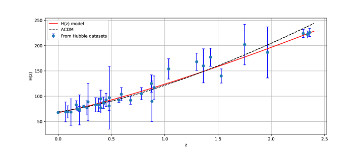
Figure 1: Error bar plot of $H$ vs $z$ for our model (red curve) and the $\Lambda$CDM model (black dotted curve). The blue dots represent the 31 Hubble data points.

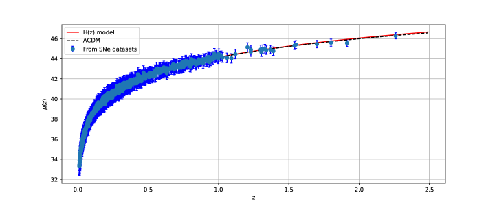
Figure 2: Error bar plot of $\mu$ vs $z$ for our model (red curve) and the $\Lambda$CDM model (black dotted curve). The blue dots represent the 1048 pantheon points.

Table 1: Best-fit model parameter values derived from observational sources of data.

Sets of data	$H_{0}$	$A$	$q_{0}$	$\omega_{0}$
Hubble	$67.4^{+1.5}_{-1.5}$	$0.262^{+0.039}_{-0.039}$	$-0.369^{+0.0195}_{-0.0195}$	$-1.01445^{+0.01}_{-0.01}$
SNe Ia	$67.2^{+2.1}_{-2.2}$	$0.19^{+0.19}_{-0.18}$	$-0.405^{+0.095}_{-0.090}$	$-1.0332^{+0.01}_{-0.01}$

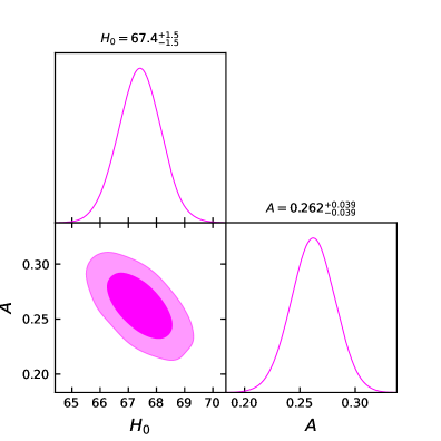
Figure 3: The confidence areas of $1-\sigma$ and $2-\sigma$ for the parameters corresponding to the Hubble sets of data.

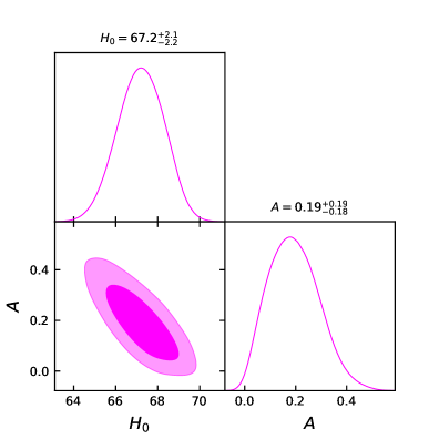
Figure 4: The confidence areas of $1-\sigma$ and $2-\sigma$ for the parameters corresponding to the SNe Ia sets of data

The observed cosmic acceleration is a new concern, according to cosmological measurements. In the absence of DE, or if its influence is negligible, the same model should decelerate in the early phase of the matter era to allow the structure formation of the cosmos. Thus, to explain the full evolutionary history of the cosmos, a cosmological model must include also a decelerated and an accelerated period of expansion. Hence, it is important to investigate the behavior of the deceleration parameter given in Eq. (29). Fig. 5 depicts the evolution of the deceleration parameter for the corresponding values of model parameters constrained by the Hubble and SNe Ia sets of data. The deceleration parameter rapidly decreases and approaches $-1$ asymptotically, indicating de-Sitter-like expansion at late time ($z\rightarrow-1$). For this scenario, the deceleration parameter represents a transition from a decelerating expansion phase (i.e. matter-dominated universe) to the current accelerating phase of the cosmos. According to Fig. 5, the value of deceleration parameter is positive at the beginning of the cosmos ($z>0$) and becomes negative at the end ($z\rightarrow-1$). The negative value of deceleration parameter denotes the accelerating expansion of the cosmos. According to recent Planck data observations, the value of deceleration parameter is in the range $-1<q<0$. As a result, our developed model is adequate for describing the late time cosmos history.

Because the model parameters $\alpha$ and $\gamma$ are not explicitly present in the calculation of the Hubble parameter (see Eq. (27)), we try to fix them to investigate the evolution of the cosmological parameters. So we used the values $\alpha=-1.053$ and $\gamma=0.5$. Eq. (20) expresses the energy density. As seen in Fig. 6, the energy density decreases with the history of the cosmos and eventually vanishes. This shows the expansion of the cosmos. Also, the pressure is expressed by Eq. (21), and its behavior is seen in Fig. 7. According to Fig. 7, the pressure p remains negative for both two values of the constrained parameters throughout the history, as predicted, indicating accelerated expansion of the cosmos.

The EoS parameter can be defined as the isotropic pressure $p$ to energy density $\rho$ ratio, i.e. $\omega=\frac{p}{\rho}$. The EoS of DE can describe cosmic inflation and accelerated expansion of the cosmos. $\omega<-\frac{1}{3}$ is the condition for an accelerating cosmos. In the most basic example, $\omega=-1$ is according to the cosmological constant, $\Lambda$CDM. Furthermore, the values of EoS $\omega=\frac{1}{3}$ and $\omega=0$ indicate a radiation-dominated cosmos and a matter-dominated cosmos, respectively. If, $-1<\omega<-\frac{1}{3}$, it represents quintessence model and $\omega<-1$ shows phantom behavior of the model. Fig. 8 depicts the behavior of the effective EoS parameter for the parameters constrained by the Hubble and SNe Ia sets of data. It is clear that the best fit value of the model parameters supports a crossing of the phantom divide line i.e. $\omega_{eff}=-1$ from $\omega_{eff}>-1$ (quintessence phase) to $\omega_{eff}<-1$ (phantom phase). Also, the current values of the EoS parameter are presented in Tab. 1. These values clearly show that the present cosmos is an accelerating phase and lies in the phantom phase. Thus, these results are consistent with several cosmological models that have been proposed in the literature [60, 61, 62].

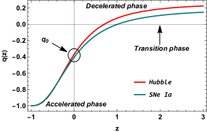
Figure 5: Curve of the deceleration parameter for the proposed model, according to the values of the parameters constrained by the Hubble, and SNe Ia sets of data.

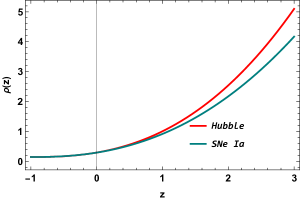
Figure 6: Curve of the energy density for the proposed model, according to the values of the parameters constrained by the Hubble, and SNe Ia sets of data.

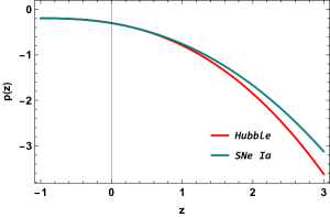
Figure 7: Curve of the pressure for the proposed model, according to the values of the parameters constrained by the Hubble, and SNe Ia sets of data.

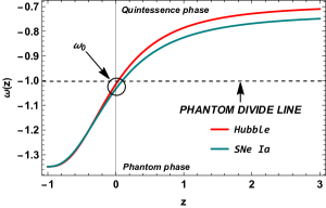
Figure 8: Curve of the effective EoS parameter for the proposed model, according to the values of the parameters constrained by the Hubble, and SNe Ia sets of data.

V Energy conditions

The physical parameters which include the deceleration parameter and the EoS parameter are important in the study of the cosmos. Now, another major research in current cosmology is on energy conditions (ECs) derived from Raychaudhuri’s equation [63]. ECs provide an important advantage in the GR for gaining a wide knowledge of the space-time singularity theorem. Capozziello et al. [64] described in great detail the generalized ECs in extended theories of gravity. They presented ECs in this article by contracting timelike and null vectors with regard to the Ricci, Einstein, and energy-momentum tensors. Capozziello and Laurentis [65], in addition to Capozziello et al. [66], presented a very comprehensive description of the ECs in modified gravity theories. The main objective of these ECs is to examine the expansion of the cosmos. There are several types of ECs, namely null energy condition (NEC), weak energy condition (WEC), dominant energy condition (DEC), and strong energy condition (SEC). These ECs are given in Weyl-type $f(Q,T)$ modified theory of gravity with defined energy density $\rho$ and pressure $p$ as follows: (a) NEC: $\rho+p\geq 0$. The violation of the NEC results in the violation of the second law of thermodynamics. The NEC is violated if $\omega$ is in phantom region $\omega<-1$. (b) WEC: $\rho\geq 0,\rho+p\geq 0$. This condition for energy density decreases. (c) DEC: $\rho\geq 0,\rho\pm p\geq 0$. (d) SEC: $\rho+p\geq 0,\rho+3p\geq 0$. The violation of NEC leads in the violation of residual ECs, which symbolizes the decrease of energy density with the expansion of the cosmos. Further, the violation of SEC indicates the acceleration of the cosmos.

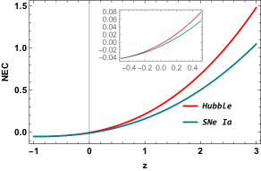
Figure 9: Curve of the NEC for the proposed model, according to the values of the parameters constrained by the Hubble, and SNe Ia sets of data.

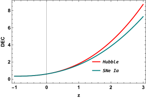
Figure 10: Curve of the DEC for the proposed model, according to the values of the parameters constrained by the Hubble, and SNe Ia sets of data.

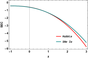
Figure 11: Curve of the SEC for the proposed model, according to the values of the parameters constrained by the Hubble, and SNe Ia sets of data.

Figs. 9, 10, and 11 show graphs of ECs with respect to redshift for Weyl-type $f(Q,T)$ gravity, and we can also see that $\rho-p\geq 0$, which indicates the DEC is satisfied. In addition, Figs. 9 and 11 show that $\rho+p\leq 0$ and $\rho+3p\leq 0$ at $z=0$ (present), leads in a violation of the NEC and SEC, respectively. As a result, a violation of the SEC causes the cosmos to accelerate and behaves like phantom model.

VI Cosmic jerk parameter

The jerk parameter is regarded as a crucial quantity for understanding the dynamics of the cosmos. The cosmic jerk parameter can define models that are near to $\Lambda$CDM. In addition, the transition from the decelerating to the accelerating phase of the cosmos is thought to be caused by a cosmic jerk. This cosmos transition happens for several models with a positive jerk parameter and a negative deceleration parameter. The value of jerk for the flat $\Lambda$CDM model is $j=1$ [67].

The cosmic jerk parameter is a dimensionless quantity that contains the third order derivative of the scale factor with regard to cosmic time and is written as,

$$j=\frac{\dddot{a}}{aH^{3}}=2q^{2}+q-\frac{\dot{q}}{H}.$$ (36)

Using Eqs. (27) and (29) in Eq. (36) we get the expression for the cosmic jerk parameter as,

$$j\left(z\right)=\frac{2A^{2}(z+1)^{2A+2}+A(z+1)^{2A+2}+1}{z^{2}(z+1)^{2A}+2z(z+1)^{2A}+(z+1)^{2A}+1}.$$ (37)

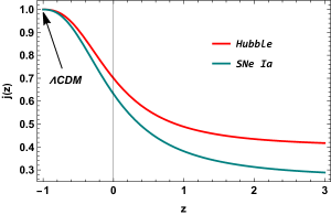
Figure 12: Curve of the cosmic jerk parameter for the proposed model, according to the values of the parameters constrained by the Hubble, and SNe Ia sets of data.

In Fig. 12, we exhibited the cosmic jerk parameter for various values of the model parameters constrained by the Hubble, and SNe Ia sets of data. One can see that the cosmic jerk parameter remains positive throughout the cosmos and is equivalent to the $\Lambda$CDM model at $z\rightarrow-1$ for the Hubble and SNe Ia sets of data. It is important to note that our model is similar to the $\Lambda$CDM model.

VII Conclusions

We proposed an accelerated cosmic model that depicts phantom behavior in the current and late stages of evolution. To begin, we derived modified Friedmann equations with an assumed form of the function $f(Q,T)$, especially $f(Q,T)=\alpha Q+\frac{\gamma}{6\kappa^{2}}T$, where $Q$ represents the non-metricity scalar of space-time in the standard Weyl form, completely specified by the Weyl vector $w_{\mu}$, and $T$ represents the trace of the matter energy-momentum tensor, and to comprehend cosmic evolution, we used a time-dependent deceleration parameter as $q=A-\frac{B}{H^{2}}$, where $A$ and $B$ are free constants. Using the previous equation for $q$, we can calculate the Hubble parameter in terms of redshift $z$. Further, we used the MCMC approach to constrain the parameters $A$ and $B$ using the Hubble, and SNe Ia sets of data. Tab. 1 shows the best-fit values for the $A$ and $B$ parameters. Then, we examined the evolution of several cosmological parameters associated with these best-fit model parameter values. The deceleration parameter in this scenario indicates a transition from a decelerating expansion phase to the current accelerating phase of the cosmos. The energy density $\rho$ of the cosmos decreases throughout time and finally vanishes. This depicts the expanding of the cosmos. Furthermore, as expected, the pressure $p$ remains negative for both two values of the constrained parameters throughout the history, indicating accelerated expansion of the cosmos. The effective EoS parameter crosses the phantom divide line i.e. $\omega_{eff}=-1$ from $\omega_{eff}>-1$ (quintessence phase) to $\omega_{eff}<-1$ (phantom phase). Furthermore, we observed that the NEC and SEC are violated, while the DEC is satisfied in Figs. 9, 10, and 11. Violation of the SEC and NEC causes the cosmos to accelerate and behaves like phantom model. Finally, to compare our model with the most widely accepted model in cosmology, we analyzed the cosmological behavior of the cosmic jerk parameter, which we observed that it remains positive throughout the cosmos and is equivalent to the $\Lambda$CDM model in the future. According to the current research, Weyl-type $f(Q,T)$ gravity with a time-dependent deceleration parameter can provide an alternative to dark energy in solving the current cosmic acceleration problem.

Data availability There are no new data associated with this article.

Declaration of competing interest The authors declare that they have no known competing financial interests or personal relationships that could have appeared to influence the work reported in this paper.

References

- [1] S. Perlmutter et al., Astrophys. J. 517, 377 (1999).
- [2] A.G. Riess et al., Astron. J. 116, 1009 (1998).
- [3] A.G. Riess et al., Astophys. J. 607, 665-687 (2004).
- [4] D.N. Spergel et al., Astrophys. J. Suppl. 148, 175 (2003).
- [5] T. Koivisto, and D.F. Mota, Phys. Rev. D 73, 083502 (2006).
- [6] S.F. Daniel, Phys. Rev. D 77, 103513 (2008).
- [7] S. Weinberg, Rev. Mod. Phys. 61, 1 (1989).
- [8] B. Ratra, and P.E.J. Peebles, Phys. Rev. D 37, 3406 (1988).
- [9] R. Caldwell, R. Dave, and P.J. Steinhardt, Phys. Rev. Lett. 80, 1582 (1998).
- [10] R.R. Caldwell, Phys. Lett. B 545, 23 (2002).
- [11] R.R. Caldwell, M. Kamionkowski, and N.N. Weinberg, Phys. Rev. Lett. 91, 071301 (2003).
- [12] G. Calcagni, and A. R. Liddle, Phys. Rev. D 74, 4 (2006).
- [13] S. Wang, Y. Wang, and M. Li, Phys. Rep. 696, 1-57 (2017).
- [14] M. Koussour, and M. Bennai, Int. J. Geom. Methods Mod., 19, 03 (2022).
- [15] M. Koussour, S. H. Shekh, M. Bennai, and T. Ouali, Chin. J. Phys. (2022). doi.org/10.1016/j.cjph.2022.11.013.
- [16] P. A. Ade et al., Astron. Astrophys. 571, A16 (2014).
- [17] H.A. Buchdahl, Month. Not. R. Astron. Soc., 150, 1 (1970).
- [18] S. Capozziello, V. F. Cardone, V. Salzano, Phys. Rev. D, 78, 063504 (2008).
- [19] A. de la Cruz-Dombriz, A. Dobado, Phys. Rev. D, 74, 087501 (2006).
- [20] S. Capozziello et al., Phys. Rev. D, 84, 043527 (2011).
- [21] Di Liu, M. J. Reboucas, Phys. Rev. D, 86, 083515 (2012).
- [22] L. Iorio, E. N. Saridakis, Month. Not. R. Astron. Soc., 427, 1555 (2012).
- [23] Deng Wang, David Mota, Phys. Rev. D, 102, 063530 (2020).
- [24] R. C. Nunes, S. Pan, E. N. Saridakis, JCAP, 08, 011 (2016).
- [25] J. B. Jimenez, L. Heisenberg, T. Koivisto, Phys. Rev. D, 98, 044048 (2018).
- [26] J. B. Jimenez et al., Phys. Rev. D, 101, 103507 (2020).
- [27] T. Harko et al., Phys. Rev. D, 98, 084043 (2018).
- [28] F. Esposito et al., Phys. Rev. D, 105, 084061 (2022).
- [29] W. Khyllep, A. Paliathanasis, Jibitesh Dutta, Phys. Rev. D, 103, 103521 (2021).
- [30] Y. Xu et al., Eur. Phys. J. C 79, 708 (2019).
- [31] S. Arora et al., Phys. Dark Univ. 30, 100664 (2020).
- [32] S. Bhattacharjee and P. K. Sahoo, Eur. Phys. J. C 80, 289 (2020).
- [33] R. Zia, D. C. Maurya and A. K. Shukla, Int. J. Geom. Methods Mod. Phys. 18, 2150051 (2021).
- [34] N. Godani and G. C. Samanta, Int. J. Geom. Methods Mod. Phys. 18 (2021).
- [35] Y. Xu et al., Eur. Phys. J. C 80, 449 (2020).
- [36] Jin-Z. Yang et al., Eur. Phys. J. C 81, 111 (2021).
- [37] G. Gadbail, S. Arora, and P.K. Sahoo, Eur. Phys. J. Plus 136, 1040 (2021).
- [38] G. Gadbail, S. Arora, and P.K. Sahoo, Eur. Phys. J. C 81, 1088 (2021).
- [39] G. N. Gadbail, S. Arora, P. Kumar, and P. K. Sahoo, Chin. J. Phys. 79, 246-255 (2022).
- [40] S. K. J. Pacif, Eur. Phys. J. Plus, 135, 10 (2020).
- [41] S. K. J. Pacif, R. Myrzakulov and S. Myrzakul, Int. J. Geom. Methods Mod., 14, 07, (2017).
- [42] N. Roy, S. Goswami and S. Das, Phys. Dark Universe, 36, 101037 (2022).
- [43] J. K. Singh and R. Nagpal, Eur. Phys. J. C, 80, 4 (2020).
- [44] A. Al Mamon and K. Bamba, Eur. Phys. J. C, 78, 10 (2018).
- [45] J. Roman-Garza et al., Eur. Phys. J. C 79, 11 (2019).
- [46] A. A. Mamon and S. Das, Eur. Phys. J. C, 77, 7 (2017).
- [47] A. Jawad, Z. Khan S. Rani, Eur. Phys. J. C, 80, 1 (2020).
- [48] D. Wang, Y. J. Yan and X. H. Meng, Eur. Phys. J. C, 77, 4 (2017).
- [49] U. Debnath and K. Bamba, Eur. Phys. J. C, 79, 8 (2019).
- [50] A. Jawad et al., Eur. Phys. J. C, 79, 11 (2019).
- [51] M. Koussour et al., Fortschr. Phys., 71, 2200172 (2023).
- [52] M. Koussour et al., Nucl. Phys. B, 978, 115738 (2022).
- [53] M. Koussour et al., Ann. Phys. 445, 169092 (2022).
- [54] D. Sofuoglu et al., Physics 4, 4 (2022).
- [55] G. S. Sharov et V. O. Vasiliev, Mathematical Modelling and Geometry. 6, 1 (2018).
- [56] M. Scolnic et al., Astrophys. J. 859, 101 (2018).
- [57] Chang et al., Chin. Phys. C 43, 125102 (2019).
- [58] R. Tripp, Astron. Astrophys. 331, 815 (1998).
- [59] R. Kessler, and D. Scolnic, Astrophys. J. 836, 56 (2017).
- [60] P. Wu, and H. Yu, Eur. Phys. J. C 71, 2 (2011).
- [61] S. Arora, and P. K. Sahoo, Ann. Phys. 534, 8 (2022).
- [62] A. Lymperis, J. Cosmol. Astropart. Phys. 11, 018 (2022).
- [63] A. Raychaudhuri, Phys. Rev. 98, 1123 (1955).
- [64] S. Capozzeiello, F. S. Lobo, and J. P. Mimoso, Phys. Lett. B 730, 280 (2014).
- [65] S. Capozziello, and M. De Laurentis, Phys. Rep. 509, 4-5 (2011).
- [66] S. Capozzeiello, F.S. Lobo, J.P. Mimoso, Phys. Rev. D 91, 124019 (2015).
- [67] D. Rapetti, et al., Mon. Not. R. Astron. Soc., 375 1510-1520 (2007).