Cascade of vestigial orders in two-component superconductors: nematic, ferromagnetic, $s$-wave charge-4e, and $d$-wave charge-4e states

Abstract

Electronically ordered states that break multiple symmetries can melt in multiple stages, similarly to liquid crystals. In the partially-melted phases, known as vestigial phases, a bilinear made out of combinations of the multiple components of the primary order parameter condenses. Multi-component superconductors are thus natural candidates for vestigial order, since they break both the $U(1)$-gauge and also time-reversal or lattice symmetries. Here, we use group theory to classify all possible real-valued and complex-valued bilinears of a generic two-component superconductor on a tetragonal or hexagonal lattice. While the more widely investigated real-valued bilinears correspond to vestigial nematic or ferromagnetic order, the little explored complex-valued bilinears correspond to a vestigial charge-$4e$ condensate, which itself can have an underlying $s$-wave, $d_{x^{2}-y^{2}}$-wave, or $d_{xy}$-wave symmetry. To properly describe the fluctuating regime of the superconducting Ginzburg-Landau action and thus access these competing vestigial phases, we employ both a large-$N$ and a variational method. We show that while vestigial order can be understood as a weak-coupling effect in the large-$N$ approach, it is akin to a moderate-coupling effect in the variational method. Despite these distinctions, both methods yield similar results in wide regions of the parameter space spanned by the quartic Landau coefficients. Specifically, we find that the nematic and ferromagnetic phases are the leading vestigial instabilities, whereas the various types of charge-$4e$ order are attractive albeit subleading vestigial channels. The only exception is for the hexagonal case, in which the nematic and $s$-wave charge-$4e$ vestigial states are degenerate. We discuss the limitations of our approach, as well as the implications of our results for the realization of exotic charge-$4e$ states in material candidates.

I Introduction

The vast majority of phase transitions can be understood employing Landau’s concept of a symmetry-breaking order parameter $\eta$ that acquires a non-zero expectation value $\langle\eta\rangle\neq 0$ below a transition temperature $T_{c}$ – or below a threshold value of a non-thermal tuning parameter. Fluctuations above $T_{c}$, encoded in the expectation value of the bilinear $\eta^{2}$, can also be captured within the Ginzburg-Landau formalism via methods that go beyond mean-field, thus describing observable phenomena such as para-conductivity and diamagnetic fluctuations above the onset of superconductivity (1; 2; 3). The versatility of the Ginzburg-Landau approach in describing disparate systems without a detailed knowledge of the microscopic interactions involved makes it a powerful phenomenological method to assess the properties of various correlated materials.

When the order parameter has mutiple components, $\boldsymbol{\eta}=(\eta_{1},\eta_{2},\dots)$, as is the case in magnetic and superconducting phases, the quantity $\left|\boldsymbol{\eta}\right|^{2}$ is just one of many bilinears of the general form $\eta_{i}M_{ij}\eta_{j}$, each of which describes a different fluctuation mode (summation over repeated indices is implied). The matrices $M_{ij}$ defining these bilinears are constrained by the symmetries of the system, much alike the types of order parameter $\boldsymbol{\eta}$ allowed are themselves restricted by the same symmetries. While $\langle\left|\boldsymbol{\eta}\right|^{2}\rangle$ is always non-zero, since the bilinear $\eta_{i}\delta_{ij}\eta_{j}$ transforms trivially under the symmetry operations of the system (i.e. it does not break any symmetries of the system), the other bilinears $\eta_{i}M_{ij}\eta_{j}$ generally have non-trivial transformation properties. In these cases, $\left\langle\eta_{i}M_{ij}\eta_{j}\right\rangle$ can be interpreted as a symmetry-breaking composite order parameter which only acquires a non-zero value below a temperature $T^{*}\geq T_{c}$. When $T^{*}$ is larger than $T_{c}$, there is a range of temperatures $T_{c}<T<T^{*}$ in which $\left\langle\eta_{i}M_{ij}\eta_{j}\right\rangle\neq 0$ but $\langle\boldsymbol{\eta}\rangle=0$, which defines a so-called vestigial phase (4; 5; 6). This denomination is motivated by the fact that the symmetries broken by $\left\langle\eta_{i}M_{ij}\eta_{j}\right\rangle\neq 0$ correspond to a subset of the symmetries broken when the primary order parameter acquires a non-zero value, $\langle\boldsymbol{\eta}\rangle\neq 0$, i.e. the vestigial phase is a partially-melted version of the primary phase. Evidently, vestigial order is a fluctuation phenomena, whose description requires methods that go beyond the mean-field approximation. More broadly, vestigial phases are an example of intertwined orders (5), as the bilinear $\left\langle\eta_{i}M_{ij}\eta_{j}\right\rangle$ and the order parameter $\langle\boldsymbol{\eta}\rangle$ are intrinsically connected, notwithstanding the fact that they describe ordered states with different broken symmetries (for a recent review on vestigial orders, see Ref. (6)).

The idea of vestigial order is a natural generalization to electronic systems of concepts typically employed in studies of liquid crystals. As such, vestigial electronic nematicity has been widely investigated in a number of correlated materials (7), such as iron pnictides (8; 9; 10), cuprates (4; 11; 12), heavy-fermion compounds (13), and twisted moiré systems (14). Beyond that, the framework of vestigial phases has also been employed to describe a broad range of phenomena observed or proposed to occur in diverse settings (15; 16; 17; 18; 19; 20; 21; 22; 23; 24; 25; 26; 27; 28; 29; 30; 31; 32; 33; 34; 35; 36; 37; 38), from Bose-Einstein condensates of ultracold atoms in optical cavities (39) to valence-bond solid phases in quantum magnets (40). It is important to emphasize that the concept of a partially ordered state in itself is not new, as it dates back to investigations of order-by-disorder phenomena in frustrated magnets (41; 42; 43; 44; 45). A more extensive literature search reveals that, already in 1988, Golubović and Kostić employed a large-$N$ approach to a Ginzburg-Landau model for incommensurate density-waves to show that partially-ordered states, which they even dubbed “nematiclike,” are naturally expected to emerge (46). To the best of our knowledge, this work, which has somehow remained unknown to much of the community (including us), obtains for the first time some of the results that would emerge again in more recent large-$N$ studies of vestigial nematicity in cuprates and pnictides (47; 8; 10; 4; 48). Finally, we stress that our analysis of vestigial order is performed at finite temperatures. Corresponding investigations for the ground state behavior were performed in Refs. (10) and (49). At $T=0$ it is also possible that vestigial phases are affected by topological terms in the collective order-parameter field theory (50).

In this paper, we revisit the issue of vestigial orders of superconductors described by two gap functions related by a symmetry of the lattice, which we consider to be either tetragonal or hexagonal/trigonal. Quite generally, systems with multiple coupled condensates provide a fertile ground for composite orders above $T_{c}$ (51; 52). While it has been known that real-valued composite order parameters describing nematicity or ferromagnetism can condense before the onset of two-component superconductivity (22; 25; 53; 6; 29), the possibility of vestigial phases characterized by complex-valued composite order parameters, which generally describe charge-$4e$ condensates (15; 54; 30), has not been as systematically investigated. Recent works focusing primarily on nematic superconductors in hexagonal lattices have shown that charge-$4e$ order can indeed be stabilized as a vestigial phase (32; 33; 55). Here, we first apply the group-theoretical formalism introduced in Ref. (6) to the case of two-component $p$-wave, $d$-wave, and $f$-wave superconductors in a lattice with either fourfold or sixfold/threefold rotational symmetry. The superconducting ground states in these cases are either nematic or chiral as it can be obtained from a straightforward mean-field minimization of the Ginzburg-Landau action. By going beyond the real-valued nematic and ferromagnetic bilinears discussed in Ref. (6), which transform trivially within the $U(1)$ group but non-trivially within the lattice point group, our group-theoretical classification of complex-valued bilinears reveals not only $s$-wave charge-$4e$ composite order parameters (which transform non-trivially within $U(1)$ but trivially within the point group), but also even more exotic $d_{xy}$-wave and $d_{x^{2}-y^{2}}$-wave charge-$4e$ orders, which transform non-trivially within both the $U(1)$ and the point groups. Interestingly, inside each of the chiral and nematic superconducting ground states, at least one real-valued bilinear and one complex-valued bilinear are simultaneously non-zero, which suggests the possibility of both vestigial nematic/ferromagnetic order and vestigial charge-$4e$ order, thus expanding the list of systems where the elusive quartet condensate can potentially be found (56; 57; 58; 59; 60; 61; 15; 62; 54; 16; 63; 64; 30; 65; 32; 33; 55; 66).

To further investigate this possibility, we solve the Ginzburg-Landau action for the two-component superconductor via two different approaches that go beyond the mean-field approximation: the large-$N$ method and the variational method. While both have been widely employed to investigate vestigial phases arising from the condensation of real-valued composite order parameters (46; 47; 8; 10; 4; 48; 22; 11; 67), they have not been systematically used to study the competition between vestigial nematic/ferromagnetic and charge-$4e$ orders. We find that treating all possible vestigial orders on an equal footing is not possible within the large-$N$ method. This is due to the Fierz identities relating the different bilinears, which introduce an unavoidable ambiguity in the decoupling scheme of the quartic terms via Hubbard-Stratonovich auxiliary fields. By imposing some physically-motivated but ad hoc restrictions on the decoupling procedure, we obtain the leading and subleading vestigial instabilities in the parameter space spanned by the ratios between the quartic coefficients of the Ginzburg-Landau action. Quite generally, we find in every region of the phase diagram attraction in one real-valued bilinear channel and one complex-valued bilinear channel, indicating the possibility of a “cascade” of vestigial phases. Despite the viability of both channels to form vestigial phases, the leading vestigial instabilities are those associated with the real-valued bilinears, corresponding to nematic and ferromagnetic orders, whereas the vestigial instabilities associated with the charge-$4e$ states are subleading. The only exception is for the case of a hexagonal nematic superconducting state, where vestigial nematicity and vestigial $s$-wave charge-$4e$ order are degenerate – as previously reported in Ref. (32).

In distinction to the large-$N$ method, which is controlled yet limited to the regime of many order-parameter components, the uncontrolled variational approach is able to describe the proper number of order-parameter components and hence allows us to treat on an equal footing all possible composite order parameters. The key limitation of the variational approach is that it only describes weak, Gaussian fluctuations. The results obtained from the variational approach largely mirror those obtained within the large-$N$ approach, with one important difference. There are regions in the parameter space without any viable vestigial phase, i.e. the instability channels associated with the real-valued bilinears and complex-valued bilinears are all repulsive. In fact, in the variational approach, the vestigial channels are only attractive when the Landau coefficients of the squared non-trivial bilinears are at least comparable in magnitude with the Landau coefficient of the squared trivial bilinear, a behavior we dub “moderate coupling.” In contrast, in the large-$N$ approach, a vestigial instability is present regardless of how small the coefficients of the squared non-trivial bilinears are, which we identify as a “weak-coupling” behavior. Nevertheless, despite these differences, the large-$N$ and variational methods give the same results outside of these parameter-space regions in which the variational method gives no (or only one) vestigial instability. We also discuss under which conditions a vestigial instability implies a vestigial phase. In doing so, we find that the most natural extension of the variational ansatz that also includes the possibility of superconducting order does not work properly, which exposes a possible limitation of the variational approach. Finally, we explore the implications of our results for various candidate two-component superconductors, such as doped $\mathrm{Bi_{2}Se_{3}}$, twisted bilayer graphene, $\mathrm{UPt_{3}}$, $\mathrm{UTe_{2}}$, $\mathrm{Sr_{2}RuO_{4}}$, $\mathrm{URu_{2}Si_{2}}$, $\mathrm{KV_{3}Sb_{5}}$, 4Hb-$\mathrm{TaS_{2}}$, and $\mathrm{CaSn_{3}}$. We also discuss ways in which the subleading charge-$4e$ vestigial instability can be uncovered in these and other systems.

This paper is organized as follows: in Sec. II we employ a group-theoretical formalism and classify all possible real-valued and complex-valued bilinears of two-component superconductors in systems with point groups $\mathsf{D_{4h}}$ or $\mathsf{D_{6h}}$. In Sec. III, we introduce the Ginzburg-Landau actions associated with these superconducting degrees of freedom, and re-derive the mean-field phase diagram in the parameter space spanned by the quartic Landau coefficients. The properties and hierarchy of leading and subleading vestigial instabilities of this model are obtained via a large-$N$ approach in Sec. IV and a variational approach in Sec. V. Section VI is devoted to a comprehensive discussion of the results and to the conclusions. Details about the group-theoretical formalism are presented in Appendix A, whereas Appendices B, C and D contain further details about the variational approach.

II Classification of bilinears

$\mathsf{D_{4h}}$	$A_{1g}$	$B_{1g}$	$B_{2g}$	$A_{2g}$
$\Gamma_{0}^{U}\big{|}_{s}$	$\Psi^{A_{1g}}$	$\Psi^{B_{1g}}$	$\Psi^{B_{2g}}$	—
$\Gamma_{0}^{U}\big{|}_{a}$	—	—	—	$\Psi^{A_{2g}}$
$\Gamma_{+2}^{U}$	$\psi^{A_{1g}}$	$\psi^{B_{1g}}$	$\psi^{B_{2g}}$	—
$\Gamma_{-2}^{U}$	$\bar{\psi}^{A_{1g}}$	$\bar{\psi}^{B_{1g}}$	$\bar{\psi}^{B_{2g}}$	—

$\Psi^{B_{1g}}$: $d_{x^{2}\!-\!y^{2}}$-nematic $\Psi^{B_{2g}}$: $d_{xy}$-nematic $\Psi^{A_{2g}}$: ferromagnetic $\psi^{A_{1g}}$: $s$-wave charge-$4e$ $\psi^{B_{1g}}$: $d_{x^{2}\!-\!y^{2}}$-wave charge-$4e$ $\psi^{B_{2g}}$: $d_{xy}$-wave charge-$4e$ $\mathsf{D_{6h}}$ $A_{1g}$ $E_{2g}$ $A_{2g}$ $\Gamma_{0}^{U}\big{|}_{s}$ $\Psi^{A_{1g}}$ $\boldsymbol{\Psi}^{E_{2g}}$ — $\Gamma_{0}^{U}\big{|}_{a}$ — — $\Psi^{A_{2g}}$ $\Gamma_{+2}^{U}$ $\psi^{A_{1g}}$ $\boldsymbol{\psi}^{E_{2g}}$ — $\Gamma_{-2}^{U}$ $\bar{\psi}^{A_{1g}}$ $\bar{\boldsymbol{\psi}}^{E_{2g}}$ — $\boldsymbol{\Psi}^{E_{2g}}$: $\begin{pmatrix}d_{x^{2}\!-\!y^{2}}\\ d_{xy}\end{pmatrix}$-nematic $\Psi^{A_{2g}}$: ferromagnetic $\psi^{A_{1g}}$: $s$-wave charge-$4e$ $\boldsymbol{\psi}^{E_{2g}}$: $\begin{pmatrix}d_{x^{2}\!-\!y^{2}}\\ d_{xy}\end{pmatrix}$-wave charge-$4e$

Table 1: The set of $N_{\Gamma}=10$ non-zero bilinear components associated with the composite orders of the two-component superconducting order parameter $\boldsymbol{\Delta}=(\Delta_{1},\Delta_{2})$ in the cases of a tetragonal lattice (Eq. 1, left panel) and of a hexagonal lattice (Eq. 2, right panel). The rows and columns of these “multiplication tables" correspond, respectively, to the bilinear decompositions in the $U(1)$ gauge sector and in the point-group lattice sector (4)-(6). The explicit expressions for the bilinears are given in Eq. (9). Next to each multiplication table, we also identify the composites according to the type of vestigial order they promote once condensed.

Our starting point is a two-component superconducting (SC) order parameter, $\boldsymbol{\Delta}=(\Delta_{1},\Delta_{2})$, which transforms as a two-dimensional irreducible representation (IR) of the point-groups $\mathsf{D_{4h}}$ or $\mathsf{D_{6h}}$, which describe tetragonal and hexagonal lattices, respectively. In particular, we have:

$$\mathrm{tetragonal\,(\mathsf{D_{4h}})} : \mathrm{IR}(\boldsymbol{\Delta}) =E_{g}\;\mathrm{or}\;E_{u},$$ (1)

$$\mathrm{hexagonal\,(\mathsf{D_{6h}})} : \mathrm{IR}(\boldsymbol{\Delta}) =E_{1g},\;E_{2g},\;E_{1u},\mathrm{or}\;E_{2u}.$$ (2)

This parametrization can describe the $m_{l}=\pm 1$ singlet $(d_{xz},d_{yz})$-wave state ($E_{g}$ or $E_{1g}$); the $m_{l}=\pm 1$ triplet $(p_{x},p_{y})$-wave state ($E_{u}$ or $E_{1u}$); the $m_{l}=\pm 2$ singlet $(d_{x^{2}-y^{2}},d_{xy})$-wave state ($E_{2g}$); the $m_{l}=\pm 2$ triplet $(f_{x^{2}z-y^{2}z},f_{xyz})$-wave state ($E_{2u}$). These states have been proposed in a variety of materials, such as the tetragonal-lattice $\mathrm{Sr_{2}RuO_{4}}$ (68; 69) and $\mathrm{URu_{2}Si_{2}}$ (70; 71; 72), the trigonal-lattice $A_{\mathrm{x}}\mathrm{Bi_{2}Se_{3}}$ with $A=\mathrm{Cu},\,\mathrm{Nb},\,\mathrm{Sr}$ (73; 74; 75; 76; 77; 25), the hexagonal-lattice $\mathrm{UPt_{3}}$ (78; 79; 80), and the triangular-moiré superlattice twisted bilayer graphene (53; 81; 82; 83; 84; 14).

In this section, we apply the group-theoretical method outlined in Ref. (6) to comprehensively identify all bilinear combinations formed out of $\boldsymbol{\Delta}$. While previous works have focused only on real-valued bilinears, corresponding to nematic and ferromagnetic vestigial order (6; 22; 29), here we show that there is an entire family of complex-valued bilinears corresponding to different types of charge-4e superconductivity, of which the results of Ref. (32) are a special case. A summary of the results of this section is presented in Table 1, with the bilinears defined in Eqs. (7)-(8).

Consider a general order parameter parameter $\boldsymbol{\eta}=(\eta_{1},\dots,\eta_{\dim\Gamma})$ that transforms according to the IR $\Gamma$ of the group $\mathscr{G}$. The corresponding bilinear components, denoted by $C^{\ell}$, with $\ell=1,\dots,N_{\Gamma}$, can be expressed as

$$C^{\ell} =\boldsymbol{\eta}^{T}M^{\ell}\boldsymbol{\eta}.$$ (3)

Here, $M^{\ell}$ is a $\dim\Gamma\times\dim\Gamma$ matrix. Since the component $C^{\ell}$ (3) is a scalar, the matrix $M^{\ell}$ has to be symmetric [$(M^{\ell})^{T}=M^{\ell}$], which reduces the total number of bilinear components from $\dim^{2}\Gamma$ to $N_{\Gamma}=\frac{1}{2}\dim\Gamma\left(1\!+\dim\Gamma\right)$. Naturally, these components can be grouped into the IRs of the group $\mathcal{G}$ according to the product decomposition $\Gamma\otimes\Gamma=\Gamma_{0}\oplus\Gamma_{1}\oplus\dots$. The explicit bilinear components (3) are deduced from the transformation properties of $\boldsymbol{\eta}$ as shown in details in App. A.

For many condensed-matter systems of interest, the symmetry group itself is a product of two groups, $\mathcal{G}=\mathcal{G}_{\mathrm{int}}\otimes\mathcal{G}_{s}$, where $\mathcal{G}_{s}$ is a space group and $\mathcal{G}_{\mathrm{int}}$ is a continuous internal group. Indeed, this is the case for magnetic materials with negligible spin-orbital coupling, where $\mathcal{G}_{\mathrm{int}}=SU(2)$ corresponds to spin-rotational symmetry, or superconductors, where $\mathcal{G}_{\mathrm{int}}=U(1)$ is the gauge symmetry. In these cases, it suffices to classify the matrices associated with the two subspaces separately and then simply multiply them, enforcing the resulting matrix $M^{\ell}$ to be symmetric. Generally, the resulting bilinear components can be categorized into four sectors according to their subspace transformation properties. (i) They are fully symmetry-preserving, i.e. transform trivially under the operations of both subgroups. (ii-iii) They break symmetries related to only one subgroup, i.e. they transform non-trivially within one group but trivially within the other subgroup. (iv) They break symmetries related to both subgroups, i.e. they transform non-trivially under the operations of both subgroups.

For our cases of interest, Eqs. (1) and (2), it is sufficient to consider the point groups $\mathcal{G}_{p}=\mathsf{D_{4h}}$ or $\mathcal{G}_{p}=\mathsf{D_{6h}}$ rather than the space group $\mathcal{G}_{s}$, since we only consider cases where superconductivity is a uniform order that does not break translational symmetry. As explained in App. A, a (complex) superconducting order parameter transforms effectively as a “Nambu” doublet $\hat{\boldsymbol{\Delta}}=(\Delta,\bar{\Delta})$ under the $U(1)$ symmetry operations, i.e. according to a two-dimensional representation. We denote this representation as $\Gamma_{\Delta}=\Gamma_{+1}^{U}\oplus\Gamma_{-1}^{U}$, with $\Gamma_{m}^{U}$ denoting the IRs of the $U(1)$ group and $m\in\{0,\pm 1,\pm 2,\dots\}$. More generally, if an order parameter transforms as $\Gamma_{+m}^{U}\oplus\Gamma_{-m}^{U}$, it corresponds to a condensate with charge $2me$, whose condensation lowers the continuous $U(1)$ gauge symmetry to a discrete $Z_{m}$ symmetry. Thus, in this notation, the two-component superconductor $\boldsymbol{\Delta}=(\Delta_{1},\Delta_{2})$ associated with the lattice IR $E_{i}$ transforms effectively as the four-component Nambu vector $\hat{\boldsymbol{\Delta}}=(\boldsymbol{\Delta},\bar{\boldsymbol{\Delta}})$ according to $\Gamma=\Gamma_{\Delta}\otimes E_{i}$. Here, the subscript $i$ is defined as $i=\left\{g,u\right\}$ for $\mathsf{D_{4h}}$ and $i=\left\{1g,\,2g,\,1u,\,2u\right\}$ for $\mathsf{D_{6h}}$. To identify the bilinear components, we rewrite the product representation separately in the two subsectors, namely, the gauge sector and the latice sector, $\Gamma\otimes\Gamma=(\Gamma_{\Delta}\otimes\Gamma_{\Delta})\otimes(E_{i}\otimes E_{i})$. Individually, they decompose according to

$$U(1) : \Gamma_{\Delta}\otimes\Gamma_{\Delta} =\left[\Gamma_{0}^{U}\oplus\big{(}\Gamma_{+2}^{U}\oplus\Gamma_{-2}^{U}\big{)}\right]_{s}\oplus\left[\Gamma_{0}^{U}\right]_{a},$$ (4)

$$\mathsf{D_{4h}} : E_{i}\otimes E_{i} =\left[A_{1g}\oplus B_{1g}\oplus B_{2g}\right]_{s}\oplus\left[A_{2g}\right]_{a},$$ (5)

$$\mathsf{D_{6h}} : E_{i}\otimes E_{i} =\left[A_{1g}\oplus E_{2g}\right]_{s}\oplus\left[A_{2g}\right]_{a},$$ (6)

where the subscripts $s,\,a$ denote the channels associated with symmetric and antisymmetric matrices, respectively (details in App. A). For a one-component superconductor, regardless of how it transforms in the lattice sector, the bilinears are always trivial within the point group. As a result, the $N_{\Gamma_{\Delta}}=3$ bilinear components comprise the trivial combination $|\Delta|^{2}$ and the doublet $(\Delta^{2},\bar{\Delta}^{2})$, which transform according to $\Gamma_{0}^{U}$ and $\left(\Gamma_{+2}^{U}\oplus\Gamma_{-2}^{U}\right)$, respectively. While the former corresponds to superconducting fluctuations, which are present at any temperature, the latter corresponds to a charge-$4e$ superconducting order parameter, which, as discussed above, lowers the continuous $U(1)$ gauge symmetry to a discrete $Z_{2}$ one.

Going back to our two-component superconductors described by Eqs. (1) and (2), the symmetric/antisymmetric matrices resulting from the decompositions (4)-(6) allow us to identify the $N_{\Gamma}=10$ bilinear components shown in Table 1 in a straightforward way. To make the notation more transparent, real-valued bilinears (i.e. which transform trivially within $U(1)$) are denoted by $\Psi^{n}$, whereas complex-valued bilinears (i.e. which transform according to $\Gamma_{\pm 2}^{U}$) are denoted by $(\psi^{n},\bar{\psi}^{n})$; in both case, $n$ denotes the point-group IR of the bilinear. In the table, the four combinations of bilinears mentioned above are highlighted with different colors: a bilinear that is trivial in both the gauge and lattice sectors is highlighted in gray; a bilinear that is trivial in the gauge sector and non-trivial in the lattice sector is highlighted in blue; a bilinear that is non-trivial in the gauge sector and trivial in the lattice sector is highlighted in pink; and a bilinear that is non-trivial in both gauge and lattice sectors is highlighted in purple.

Explicitly, for the $\mathsf{D_{4h}}$ case (1), one obtains the trivial combination $\Psi^{A_{1g}}=\boldsymbol{\Delta}^{\dagger}\tau^{0}\boldsymbol{\Delta}$ with Pauli matrices $\tau^{i}$ ; the three real-valued non-trivial bilinears

$$\Psi^{B_{1g}} =\boldsymbol{\Delta}^{\dagger}\tau^{z}\boldsymbol{\Delta}, \Psi^{B_{2g}} =\boldsymbol{\Delta}^{\dagger}\tau^{x}\boldsymbol{\Delta}, \Psi^{A_{2g}} =\boldsymbol{\Delta}^{\dagger}\tau^{y}\boldsymbol{\Delta},$$ (7)

and the three complex-valued bilinears

$$\psi^{A_{1g}} =\boldsymbol{\Delta}^{T}\tau^{0}\boldsymbol{\Delta}, \psi^{B_{1g}} =\boldsymbol{\Delta}^{T}\tau^{z}\boldsymbol{\Delta}, \psi^{B_{2g}} =\boldsymbol{\Delta}^{T}\tau^{x}\boldsymbol{\Delta}.$$ (8)

Writing them explicitly in terms of the two SC components $\boldsymbol{\Delta}=(\Delta_{1},\Delta_{2})$ yields:

$$\Psi^{A_{1g}} =|\Delta_{1}|^{2}+|\Delta_{2}|^{2}, \psi^{A_{1g}} =\Delta_{1}^{2}+\Delta_{2}^{2},$$

$$\Psi^{A_{2g}} =\mathsf{i}\left(\bar{\Delta}_{2}\Delta_{1}-\bar{\Delta}_{1}\Delta_{2}\right),$$

$$\Psi^{B_{1g}} =|\Delta_{1}|^{2}-|\Delta_{2}|^{2}, \psi^{B_{1g}} =\Delta_{1}^{2}-\Delta_{2}^{2},$$

$$\Psi^{B_{2g}} =\bar{\Delta}_{1}\Delta_{2}+\bar{\Delta}_{2}\Delta_{1}, \psi^{B_{2g}} =2\Delta_{1}\Delta_{2}.$$ (9)

Among the real-valued composite order parameters (7), $\Psi^{A_{2g}}$ corresponds to an out-of-plane ferromagnetic moment that breaks time reversal symmetry, while $\Psi^{B_{1g}}$ and $\Psi^{B_{2g}}$ describe electronic nematicity that breaks the tetragonal symmetry of the lattice by making, respectively, the two cartesian axes inequivalent ($B_{1g}$ or $d_{x^{2}-y^{2}}$-nematic) or the two diagonals inequivalent ($B_{2g}$ or $d_{xy}$-nematic). As for the complex-valued composites in (8), all of them correspond to a type of charge-$4e$ superconductivity, as explained above. They can be further classified according to how they transform upon the point-group operations. Thus, $\psi^{A_{1g}}$ is an $s$-wave charge-$4e$ superconductor while $\psi^{B_{1g}}$ and $\psi^{B_{2g}}$ are, respectively, $d_{x^{2}-y^{2}}$-wave and $d_{xy}$-wave charge-$4e$ superconductors. For later convenience, we introduce the groups of point-group IRs associated with the real-valued (7) and the complex-valued (8) non-trivial bilinears,

$$\mathbb{G}_{\mathbb{R}} =\{A_{2g},B_{1g},B_{2g}\}, \mathbb{G}_{\mathbb{C}} =\{A_{1g},B_{1g},B_{2g}\},$$ (10)

as well as the full real group $\mathbb{G}_{\mathbb{R}}^{0}=\{A_{1g},\mathbb{G}_{\mathbb{R}}\}$ containing also the trivial lattice IR.

In the $\mathsf{D_{6h}}$ case (2), the only modication required is to combine the two $B$-channel bilinears into a single $E_{2g}$-channel bilinear:

$$\boldsymbol{\Psi}^{E_{2g}} =\big{(}\Psi^{B_{1g}},\,-\Psi^{B_{2g}}\big{)}=\big{(}\boldsymbol{\Delta}^{\dagger}\tau^{z}\boldsymbol{\Delta},\,-\boldsymbol{\Delta}^{\dagger}\tau^{x}\boldsymbol{\Delta}\big{)},$$

$$\boldsymbol{\psi}^{E_{2g}} =\big{(}\psi^{B_{1g}},\,-\psi^{B_{2g}}\big{)}=\big{(}\boldsymbol{\Delta}^{T}\tau^{z}\boldsymbol{\Delta},\,-\boldsymbol{\Delta}^{T}\tau^{x}\boldsymbol{\Delta}\big{)}.$$ (11)

To make the presentation more transparent, hereafter we will only derive the results for the $\mathsf{D_{4h}}$ case (1) and just mention the replacements necessary to recover the results for the $\mathsf{D_{6h}}$ case (2).

III Superconducting phase diagram: Ginzburg-Landau theory

To keep the analysis general, in this paper we use a Ginzburg-Landau formalism to obtain the phase diagrams of the two-component superconducting order parameters $\boldsymbol{\Delta}=(\Delta_{1},\Delta_{2})$ of Eqs. (1) and (2). Since the values of the Landau coefficients depend on the microscopic model, we will consider the entire parameter space spanned by the Landau coefficients. Our only restriction is that the free energy is bounded, i.e. that the underlying superconducting transition is second-order. The Ginzburg-Landau expansion for the superconducting action can be expressed as (see, for instance, Ref. (85))

$$\mathcal{S} =\int_{\mathsf{x}}r_{0}\,\boldsymbol{\Delta}^{\dagger}\boldsymbol{\Delta}\;+\;\mathcal{S}^{\mathrm{grad}}+\;\mathcal{S}^{\mathrm{int}}\,,$$ (12)

where the variable $\mathsf{x}=(\tau,\boldsymbol{r})$ comprises both imaginary time and position, and the $\boldsymbol{\Delta}(\mathsf{x})$ dependence is left implicit. The quadratic coefficient is $r_{0}=a_{0}(T-T_{0})$ with $a_{0}>0$ and $T_{0}>0$ denoting the bare superconducting transition. The gradient ($\mathcal{S}^{\mathrm{grad}}$) and interaction ($\mathcal{S}^{\mathrm{int}}$) contributions to the action depend on the point-group symmetry. For the $\mathsf{D_{4h}}$ tetragonal case (1), the interaction term is given, in terms of the bilinears (7), by

$$\mathcal{S}^{\mathrm{int}} =\int_{\mathsf{x}}\Big{[}u\,\big{(}\Psi^{A_{1g}}\big{)}^{2}+v\,\big{(}\Psi^{A_{2g}}\big{)}^{2}+w\,\big{(}\Psi^{B_{1g}}\big{)}^{2}\Big{]},$$ (13)

where the interaction parameters $u$, $v$, and $w$ have to satisfy $u>0$, $v>-u$ and $w>-u$ in order for the action to be bounded. Note that the interaction term can only have squared bilinears as it must transform trivially. The gradient term, which is essential to account for order parameter fluctuations, is more conveniently expressed in momentum space,

$$\mathcal{S}^{\mathrm{grad}} =\frac{T}{V}\sum_{k}\boldsymbol{\Delta}_{k}^{\dagger}\left(f_{\boldsymbol{k}}^{A_{1g}}\tau^{0}\!+\!f_{\boldsymbol{k}}^{B_{1g}}\tau^{z}\!+\!f_{\boldsymbol{k}}^{B_{2g}}\tau^{x}\right)\boldsymbol{\Delta}_{k},$$ (14)

where we defined the Fourier transform $\boldsymbol{\Delta}_{k}=\frac{T}{V}\int d\mathsf{x}\>\boldsymbol{\Delta}(\mathsf{x})e^{-ik\mathsf{x}}$ with the volume $V$ and the variable $k=(\omega_{n},\boldsymbol{k})$ comprising bosonic Matsubara frequency $\omega_{n}=2\pi nT$ and momentum $\boldsymbol{k}$. In the continuum limit, the gradient functions in (14) are given by:

$$f_{\boldsymbol{k}}^{A_{1g}} =\mathsf{d}_{0}(k_{x}^{2}+k_{y}^{2})+\mathsf{d}_{z}k_{z}^{2}, f_{\boldsymbol{k}}^{B_{1g}} =\mathsf{d}_{1}(k_{x}^{2}-k_{y}^{2}),$$

$$f_{\boldsymbol{k}}^{B_{2g}} =\mathsf{d}_{2}2k_{x}k_{y},$$ (15)

where $\mathsf{d}_{i}$ are stiffness coefficients.

The $\mathsf{D_{6h}}$ hexagonal case (2) is obtained by setting $w=0$ and $\mathsf{d}_{2}=\mathsf{d}_{1}$ in Eqs. (13) and (14), respectively. Note that for other point groups that have threefold rotational symmetry, additional gradient terms may be allowed. For instance, for the trigonal $\mathsf{D_{3d}}$ group, which describes the lattice symmetries of $A_{\mathrm{x}}\mathrm{Bi_{2}Se_{3}}$, the two extra terms, $\mathsf{d}_{3}2k_{y}k_{z}$ and $\mathsf{d}_{3}2k_{x}k_{z}$, must be added to $f_{\boldsymbol{k}}^{B_{1g}}$ and $f_{\boldsymbol{k}}^{B_{2g}}$, respectively, as explained in Ref. (25).

Before discussing the emergence of vestigial phases, we do a mean-field calculation to obtain the superconducting phase diagram of the Ginzburg-Landau action in Eq. (12). The results are well known (85): minimization of the action gives three distinct states, as shown in Fig. 1(a). For $w,v>0$ the superconducting ground state is $\langle\boldsymbol{\Delta}\rangle\sim(1,1)$, which we denote as the $d_{xy}$-nematic (or $B_{2g}$-nematic) SC state. It not only breaks the $U(1)$ gauge symmetry, but also the fourfold rotational symmetry of $\mathsf{D_{4h}}$ by making the two diagonals inequivalent. Indeed, substituting $\langle\boldsymbol{\Delta}\rangle\sim(1,1)$ into the real-valued bilinear expressions (7), we find that only the $d_{xy}$-nematic (or $B_{2g}$-nematic) composite order parameter $\langle\Psi^{B_{2g}}\rangle$ is non-zero in this phase. As for the complex-valued bilinears in Eq. (8), two charge-$4e$ composite order parameters are non-zero in this phase, namely, the $s$-wave $\langle\psi^{A_{1g}}\rangle$ and the $d_{xy}$-wave $\langle\psi^{B_{2g}}\rangle$.

In the region $w<\min(0,v)$ of the parameter space spanned by the quartic Landau coefficients, the superconducting ground state is $\langle\boldsymbol{\Delta}\rangle\sim(1,0)$, which corresponds to a $d_{x^{2}-y^{2}}$-nematic (or $B_{1g}$-nematic) superconductor. In this case, tetragonal symmetry is broken due to the inequivalence between the horizontal and vertical Cartesian axes. The corresponding non-zero composite order parameters are the $d_{x^{2}-y^{2}}$-nematic (or $B_{1g}$-nematic) $\langle\Psi^{B_{1g}}\rangle$, the $s$-wave charge-$4e$ $\langle\psi^{A_{1g}}\rangle$, and the $d_{x^{2}-y^{2}}$-wave charge-$4e$ $\langle\psi^{B_{1g}}\rangle$. Finally, in the region $v<\min(0,w)$, the ground state is the chiral superconductor $\langle\boldsymbol{\Delta}\rangle\sim(1,\mathsf{i})$. This is a time-reversal symmetry-breaking (TRSB) phase that respects all symmetries of the tetragonal lattice. The associated composite order parameters are the ferromagnetic $\langle\Psi^{A_{2g}}\rangle$, the $d_{x^{2}-y^{2}}$-wave charge-$4e$ $\langle\psi^{B_{1g}}\rangle$, and the $d_{xy}$-wave charge-$4e$ $\langle\psi^{B_{2g}}\rangle$.

While it is straightforward to verify which non-trivial bilinears are non-zero by simply substituting the superconducting solutions in Eqs. (7) and (8), valuable insight can be obtained directly from the interaction action, Eq. (13). Indeed, we can loosely interpret the interaction action, which is quartic in the superconducting order parameters, as an effective action that is quadratic in the bilinears. This suggests, for instance, that $w<0$ should favor the condensation of $\langle\Psi^{B_{1g}}\rangle$, whereas $v<0$ should promote $\langle\Psi^{A_{2g}}\rangle\neq 0$. At first sight, this oversimplified analysis would seem to suggest that no composite orders would condense when $w,v>0$. To see why this is not the case, we use the fact that

$$\big{(}\Psi^{A_{1g}}\big{)}^{2}=\big{(}\Psi^{B_{1g}}\big{)}^{2}+\big{(}\Psi^{B_{2g}}\big{)}^{2}+\big{(}\Psi^{A_{2g}}\big{)}^{2},$$ (16)

to rewrite the interaction action as:

$$\mathcal{S}^{\mathrm{int}}=\int_{\mathsf{x}}\left[\left(u+w\right)\big{(}\Psi^{A_{1g}}\big{)}^{2}+\left(v-w\right)\big{(}\Psi^{A_{2g}}\big{)}^{2}-w\,\big{(}\Psi^{B_{2g}}\big{)}^{2}\right].$$ (17)

Thus, $w>0$ should favor the condensation of $\langle\Psi^{B_{2g}}\rangle$. Equation (16) is an example of a so-called Fierz identity. The complete list of Fierz identities in our case is:

$$\big{(}\Psi^{A_{1g}}\big{)}^{2} =\sum_{n\in\mathbb{G}_{\mathbb{R}}}\left(\Psi^{n}\right)^{2}, \big{(}\Psi^{A_{1g}}\big{)}^{2} =\left|\psi^{B_{1g}}\right|^{2}+\big{(}\Psi^{B_{2g}}\big{)}^{2},$$

$$\big{(}\Psi^{A_{1g}}\big{)}^{2} =\left|\psi^{A_{1g}}\right|^{2}+\big{(}\Psi^{A_{2g}}\big{)}^{2}, \big{(}\Psi^{A_{1g}}\big{)}^{2} =\left|\psi^{B_{2g}}\right|^{2}+\big{(}\Psi^{B_{1g}}\big{)}^{2}.$$ (18)

The Fierz identities imply that the representation of the interaction action (13) in terms of the three bilinear channels $\Psi^{A_{1g}}$, $\Psi^{A_{2g}}$ and $\Psi^{B_{1g}}$ is not unique. On the contrary, by inserting these identities in the interaction action (13), it can be represented in terms of infinitely many combinations of composite bilinears. Note that the mean-field results are insensitive to this choice of representation of the quartic action.

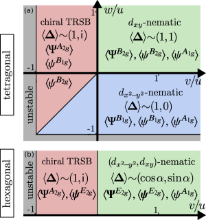
Figure 1: Mean-field phase diagram, in the parameter space spanned by the quartic Landau coefficients of Eq. (12), of the two-component superconducting pairing states of the (a) tetragonal case $\mathsf{D_{4h}}$ (1) and (b) hexagonal case $\mathsf{D_{6h}}$ (2). In each phase, we show the relationship between the two components of the superconducting order parameter, $\boldsymbol{\Delta}=(\Delta_{1},\Delta_{2})$, as well as all non-zero bilinears defined in Eqs. (7)-(8). Each phase is labeled by the additional symmetry that they break besides the $U(1)$ gauge symmetry, which could be time-reversal symmetry (TRS) or a point-group symmetry. In the regions labeled “unstable” (dark-gray), the action is unbounded.

The superconducting phase diagram in the case of a two-component order parameter defined on the $\mathsf{D_{6h}}$ lattice according to Eq. (2) is obtained by setting $w=0$ in Eq. (13) and then minimizing the action. There are two distinct ground states, as shown in Fig. 1(b). For $v<0$, we obtain the chiral state $\langle\boldsymbol{\Delta}\rangle\sim(1,\mathsf{i})$ and non-zero composite order parameters $\langle\Psi^{A_{2g}}\rangle$ and $\langle\boldsymbol{\psi}^{E_{2g}}\rangle$. For $v>0$, the superconducting ground state is the nematic one, $\langle\boldsymbol{\Delta}\rangle\sim(\cos\alpha,\sin\alpha)$, which is accompanied by the non-zero composite order parameters $\langle\boldsymbol{\Psi}^{E_{2g}}\rangle$, $\langle\psi^{A_{1g}}\rangle$ and $\langle\boldsymbol{\psi}^{E_{2g}}\rangle$. Note that the continuous degeneracy of the nematic superconducting state, indicated by the angle $\alpha$, is an artifact of stopping the Ginzburg-Landau at fourth order. Addition of the sixth order term $\mathcal{S}_{6}=u_{6}\Psi^{E_{2g},1}\Big{[}\big{(}\Psi^{E_{2g},1}\big{)}^{2}-3\big{(}\Psi^{E_{2g},2}\big{)}^{2}\Big{]}$ reduces the degeneracy to threefold, as one would have expected for a system with threefold rotational symmetry (85; 73; 53). For completeness, we also list the Fierz identities for the $\mathsf{D_{6h}}$ case, noting that $\left|\boldsymbol{\Psi}^{E_{2g}}\right|^{2}=\big{(}\Psi^{E_{2g},1}\big{)}^{2}+\big{(}\Psi^{E_{2g},2}\big{)}^{2}$,

$$\big{(}\Psi^{A_{1g}}\big{)}^{2} \!=\big{(}\Psi^{A_{2g}}\big{)}^{2}\!+\left|\boldsymbol{\Psi}^{E_{2g}}\right|^{2}\!, 2\big{(}\Psi^{A_{1g}}\big{)}^{2} =\left|\boldsymbol{\Psi}^{E_{2g}}\right|^{2}\!+\left|\boldsymbol{\psi}^{E_{2g}}\right|^{2}\!,$$

$$\big{(}\Psi^{A_{1g}}\big{)}^{2} \!=\big{(}\Psi^{A_{2g}}\big{)}^{2}\!+\left|\psi^{A_{1g}}\right|^{2}\!.$$ (19)

The results of this section reveal that each superconducting ground state is accompanied by several non-zero non-trivial bilinears. For instance, in the case of the $\mathsf{D_{4h}}$ lattice, each superconducting state has one real-valued (corresponding to nematicity or ferromagnetism) and two complex-valued (corresponding to charge-$4e$ superconductivity) non-zero bilinears. In a mean-field approach, these composite order parameters condense simultaneously and along with superconductivity. However, as we discuss in the next sections, fluctuations may allow them to condense before the onset of superconductivity, giving rise to vestigial phases.

IV Vestigial-orders phase diagram: large-$N$ approach

As discussed in the previous section, it is necessary to go beyond the mean-field approximation in order to assess whether a vestigial phase, characterized by a non-zero composite order $\left\langle\Psi^{n}\right\rangle\neq 0$ or $\left\langle\psi^{n}\right\rangle\neq 0$, can emerge before the onset of superconductivity, i.e. $\langle\boldsymbol{\Delta}\rangle=0$. Fluctuations can be accounted for via different approaches. For instance, renormalization-group (RG) methods have been widely used to study actions of the form (12) (86; 87; 10; 88). An interesting outcome of a $\left(4-\varepsilon\right)$ RG calculation is that the mean-field phase boundaries obtained in Fig. 1 remain unchanged (88). However, to the best of our knowledge, a consistent RG scheme that treats the vestigial orders on an equal footing as the primary order has yet to be established.

Here, we focus on the large-$N$ approach, which has been widely employed to search for vestigial phases (46; 47; 8; 10; 4; 48). The underlying assumption is that the number of order parameter components can be extended from a given value $N_{0}$ ($N_{0}=2$ in the present case) to an arbitrary $N\gg 1$. The key point is that, in the $N\rightarrow\infty$ limit, the partition function associated with the action (12), $\mathcal{Z}=\int D\boldsymbol{\Delta}\,\exp\left(-S\left[\boldsymbol{\Delta}\right]\right)$, can be computed exactly. The procedure consists of performing Hubbard-Stratonovich transformations of the quartic terms of the action by introducing appropriate auxiliary fields. The resulting action is quadratic in the $\boldsymbol{\Delta}$ fields, and the calculation of the partition function reduces to the straightforward evaluation of a Gaussian functional integral. The remaining functional integral over the auxiliary fields can be evaluated exactly in the $N\rightarrow\infty$ limit via the saddle-point method. This leads to self-consistent equations for the uniform auxiliary fields, which can then be solved to determine whether any symmetry-breaking auxiliary field can condense still in the fluctuating regime of the $\boldsymbol{\Delta}$ field (for more details on the large-$N$ method, see Refs. (46; 47; 8; 10; 4; 48)). Note that while this method is controlled in the small parameter $1/N$, there is no guarantee that the physical case $N_{0}$ is captured by this expansion. While the large-$N$ method has been previously used to investigate vestigial phases, the focus has been extensively on the real bilinears only. Our goal in this section is to extend this method to also include the complex bilinears.

By writing the quartic action in the form of Eq. (13), it is natural to use the bilinears $\Psi^{A_{1g}}$, $\Psi^{A_{2g}}$, and $\Psi^{B_{1g}}$ to introduce the Hubbard-Stratonovich fields. The resulting self-consistent equations, however, will not bring any information about the complex bilinears $\psi^{n}$. Self-consistent equations for the latter could be obtained by exploiting the Fierz identities (18). But the issue is that these identities can be used to generate an infinite number of bilinear representations for the quartic terms of the action, rendering a simultaneous analysis of all possible vestigial orders intractable. This issue is well known in Hartree-Fock-like solutions of interacting fermionic Hamiltonians, since one only has access to the particular channels in which the interactions are decomposed. Despite these shortcomings, there is still useful information about the vestigial orders that can be obtained from the large-$N$ approach, as we discuss below. Note that some of the results obtained in this section recover results previously reported elsewhere (46; 47; 8; 10; 4; 48).

IV.1 Derivation of the self-consistent equations

We start by considering an arbitrary representation of the interaction action in terms of the bilinears of $\boldsymbol{\Delta}$:

$$\mathcal{S}^{\mathrm{int}} =\frac{1}{N}\int_{\mathsf{x}}\Big{[}\sum_{n\in\mathbb{G}_{\mathbb{R}}^{0}}U_{n}\,(\Psi^{n})^{2}+\sum_{n\in\mathbb{G}_{\mathbb{C}}}u_{n}\,|\psi^{n}|^{2}\Big{]}\,.$$ (20)

Here, the coefficients $U_{n}$ and $u_{n}$, which we dub interaction parameters, are functions of the quartic Landau coefficients $u$, $v$, and $w$ that depend on the particular representation chosen. For example, for the representation shown in Eq. (13), there are only three non-zero parameters: $U_{A_{1g}}=u$, $U_{A_{2g}}=v$ and $U_{B_{1g}}=w$. Quite generally, only a subset of all possible $U_{n}$ and $u_{n}$ will be non-zero for a given representation. Nevertheless, to keep the formalism general, we will keep them undetermined for now. We perform the Hubbard-Stratonovich transformations

$$1 =\prod_{n\in\mathbb{G}_{\mathbb{R}}^{0}}\!\int\!\mathcal{D}\Phi^{n}\,\text{exp}\Big{[}\frac{N}{4U_{n}}\!\int_{\mathsf{x}}\!\Big{(}\Phi^{n}-\frac{2U_{n}}{N}\Psi^{n}\Big{)}^{2}\Big{]}\,,$$ (21)

$$1 =\prod_{n\in\mathbb{G}_{\mathbb{C}}}\!\int\!\mathcal{D}\!\left(\phi^{n},\bar{\phi}^{n}\right)\,\text{exp}\Big{[}\frac{N}{4u_{n}}\!\int_{\mathsf{x}}\Big{|}\phi^{n}-\frac{2u_{n}}{N}\psi^{n}\Big{|}^{2}\Big{]}\,,$$ (22)

to decouple the interaction action, which results in the introduction of the auxiliary bosonic fields $\Phi^{n}$ and $\phi^{n}$. The action then becomes

$$\mathcal{S}_{N} =N\mathcal{S}_{0}+\frac{1}{2}\frac{V}{T}\sum_{k,k^{\prime}}\hat{\boldsymbol{\Delta}}_{k}^{\dagger}\,\,\mathcal{G}_{k,k^{\prime}}^{-1}\,\,\hat{\boldsymbol{\Delta}}_{k^{\prime}}\,,$$ (23)

where we introduced the momentum-space Nambu vector $\hat{\boldsymbol{\Delta}}_{k}=\left(\boldsymbol{\Delta}_{k},\bar{\boldsymbol{\Delta}}_{-k}\right)$. Here, $\mathcal{S}_{0}$ depends only quadratically on the auxiliary fields

$$\mathcal{S}_{0} =-\sum_{n\in\mathbb{G}_{\mathbb{R}}^{0}}\frac{V}{4TU_{n}}\sum_{k}|\Phi_{k}^{n}|^{2}-\sum_{n\in\mathbb{G}_{\mathbb{C}}}\frac{V}{4Tu_{n}}\sum_{k}|\phi_{k}^{n}|^{2},$$ (24)

and the Nambu Green’s function is given by

$$\mathcal{G}_{k,k^{\prime}}^{-1} =2r_{0}\delta_{kk^{\prime}}M^{A_{1g}}+2\sum_{n\in\mathbb{G}_{\mathbb{R}}^{0}}\left[f_{\boldsymbol{k}}^{n}\delta_{kk^{\prime}}+\Phi_{k-k^{\prime}}^{n}\right]M^{n}$$

$$\quad+\sum_{n\in\mathbb{G}_{\mathbb{C}}}\left[\phi_{k-k^{\prime}}^{n}(m^{n})^{\dagger}+\mathrm{h.c.}\right].$$ (25)

where we defined the $M^{n}$, $m^{n}$ matrices (see Appendix A):

$$M^{A_{1g}} =\tau^{0}\sigma^{0}/2, m^{A_{1g}} =\tau^{0}\sigma^{-}, M^{A_{2g}} =\tau^{y}\sigma^{z}/2,$$

$$M^{B_{1g}} =\tau^{z}\sigma^{0}/2, m^{B_{1g}} =\tau^{z}\sigma^{-},$$

$$M^{B_{2g}} =\tau^{x}\sigma^{0}/2, m^{B_{2g}} =\tau^{x}\sigma^{-},$$ (26)

with $\sigma^{\pm}=(\sigma^{x}\pm\mathsf{i}\sigma^{y})/2$. The form factors $f_{\boldsymbol{k}}^{n}$ are given by Eq. (15) and $f_{\boldsymbol{k}}^{A_{2g}}=0$. Since the action (23) is Gaussian in the superconducting field $\boldsymbol{\Delta}$, the corresponding integration in the partition function can be carried out, leading to an effective action that depends only on the auxiliary fields

$$\mathcal{S}_{\mathrm{eff}} =N\Big{\{}\mathcal{S}_{0}+\frac{1}{4}\text{Tr}\log\left(\mathcal{G}^{-1}\right)\Big{\}}\,,$$ (27)

where we dropped an unimportant constant. Importantly, the expectation values of the bilinear combinations $\Psi^{n}$, $\psi^{n}$ are directly proportional to the expectation values of the auxiliary fields via

$$\langle\Psi^{n}\rangle =\frac{N}{2U_{n}}\langle\Phi^{n}\rangle_{\Phi}, \langle\psi^{n}\rangle =\frac{N}{2u_{n}}\langle\phi^{n}\rangle_{\Phi}.$$ (28)

Therefore, we identify the auxiliary fields as composite order parameters. Note that we carefully distinguish the usual expectation value obtained by integrating over $\int\!\mathcal{D}\!\left(\boldsymbol{\Delta},\bar{\boldsymbol{\Delta}}\right)$ and the expectation value with respect to the auxiliary fields $\langle\mathcal{O}\rangle_{\Phi}=\mathcal{Z}_{\Phi}^{-1}\int\!\mathcal{D}\!\left(\Phi^{n},\phi^{n},\bar{\phi}^{n}\right)\mathcal{O}\exp\left[-\mathcal{S}_{\mathrm{eff}}\right]$, where $\mathcal{Z}_{\Phi}$ is the contribution to the partition function that depends on the auxiliary fields only.

In the limit $N\rightarrow\infty$, the prefactor $N$ in Eq. (27) justifies a saddle-point analysis. Technically, this means that we expand the effective action (27) up to second order around the homogeneous field values $\Phi_{0}^{n}$ and $\phi_{0}^{n}$ that extremize $\mathcal{S}_{\mathrm{eff}}$:

$$\mathcal{S}_{\mathrm{eff}} \approx\mathcal{S}_{\mathrm{eff}}\big{|}_{0}+\frac{1}{2}\sum_{j,j^{\prime}}\int_{\mathsf{x},\mathsf{x}^{\prime}}\frac{\partial^{2}\mathcal{S}_{\mathrm{eff}}}{\partial X_{j}(\mathsf{x})\partial X_{j^{\prime}}(\mathsf{x}^{\prime})}\Big{|}_{0}\quad\times$$

$$\qquad\qquad\qquad\,\left(X_{j}(\mathsf{x})-X_{j0}\right)\left(X_{j^{\prime}}(\mathsf{x}^{\prime})-X_{j^{\prime}0}\right).$$ (29)

For the sake of compactness, we used a single variable $\boldsymbol{X}=\big{(}\Phi^{n},\phi^{n},\bar{\phi}^{n}\big{)}$ to denote all composite fields. The Gaussian form (29) allows for a direct evaluation of the expectation values (28), yielding, to leading order,

$$\langle\Phi^{n}\rangle_{\Phi} =\Phi_{0}^{n}, \langle\phi^{n}\rangle_{\Phi} =\phi_{0}^{n}.$$ (30)

Thus, Eqs. (30) and (28) imply that the homogeneous fields ($\Phi_{0}^{n}$, $\phi_{0}^{n}$) are the composite order parameters associated with the non-trivial superconducting bilinear combinations (7)-(8). By definition, the homogeneous values $\Phi_{k}^{n}=\Phi_{0}^{n}\delta_{k,0}$ and $\phi_{k}^{n}=\phi_{0}^{n}\delta_{k,0}$ are given by $\frac{\partial\mathcal{S}_{\mathrm{eff}}}{\partial X_{j}}\big{|}_{0}=0$, yielding the saddle-point equations

$$r_{0}-R_{0} =-2U_{A_{1g}}\Pi^{A_{1g}},$$ (31)

$$\Phi_{0}^{n} =2U_{n}\Pi^{n}, \!\!n \in\mathbb{G}_{\mathbb{R}},$$ (32)

$$\phi_{0}^{n} =2u_{n}\pi^{n}, \!\!n \in\mathbb{G}_{\mathbb{C}}.$$ (33)

Here, we have introduced the renormalized mass parameter $R_{0}\equiv r_{0}+\Phi_{0}^{A_{1g}}$, as well as the integrals

$$\Pi^{n} =\frac{T}{2V}\!\sum_{k}\!\mathrm{tr}\left[\mathcal{G}_{k,k}M^{n}\right], \pi^{n} =\frac{T}{2V}\!\sum_{k}\!\mathrm{tr}\left[\mathcal{G}_{k,k}m^{n}\right],$$ (34)

with $n\in\mathbb{G}_{\mathbb{R}}^{0}$ and $n\in\mathbb{G}_{\mathbb{C}}$, respectively. The solution of the coupled saddle-point equations (31)-(33) determines the renormalized mass $R_{0}$ and the set of composite order parameters $\big{(}\Phi_{0}^{n},\phi_{0}^{n}\big{)}$ for a given reduced temperature $r_{0}$. It is important to notice that equations (32)-(33) can only have a non-zero solution for $\big{(}\Phi_{0}^{n},\phi_{0}^{n}\big{)}$ if the corresponding interaction parameter is negative ($U_{n},u_{n}<0$), i.e. if that particular vestigial-order channel is attractive.

IV.2 Hierarchy of vestigial orders

The onset of a non-zero $\big{(}\Phi_{0}^{n},\phi_{0}^{n}\big{)}$ via a continuous transition in the regime where the primary order parameter vanishes implies the existence of a vestigial phase. Of course, if the composite transition is first-order, it may trigger a simultaneous transition in the superconducting channel; we will get back to this point in Sec. V.4. To identify the leading vestigial instability, we determine the highest critical temperature associated with each composite order parameter. This is achieved by computing the respective composite-order susceptibilities, which can be evaluated in a straightforward way by means of the expansion (29):

$$\chi_{\Psi^{n}}^{\!}(R_{0}) =\frac{\chi_{\Psi^{n}}^{(0)}}{1+2U_{n}\chi_{\Psi^{n}}^{(0)}}, \chi_{\psi^{n}}^{\!}(R_{0}) =\frac{\chi_{\psi^{n}}^{(0)}}{1+2u_{n}\chi_{\psi^{n}}^{(0)}}.$$ (35)

Here, we defined the bare susceptibilities as

$$\chi_{\Psi^{n}}^{(0)} =-\frac{\partial\Pi^{n}}{\partial\Phi_{0}^{n}}\big{|}_{\Phi_{0}^{n}=\phi_{0}^{n}=0}=\frac{T}{V}\sum_{k}\mathrm{tr}\left[\mathcal{G}_{k}^{0}M^{n}\mathcal{G}_{k}^{0}M^{n}\right],$$ (36)

$$\chi_{\psi^{n}}^{(0)} =-\frac{\partial\pi^{n}}{\partial\phi_{0}^{n}}\big{|}_{\Phi_{0}^{n}=\phi_{0}^{n}=0}=\!\frac{T}{2V}\!\sum_{k}\!\mathrm{tr}\left[\mathcal{G}_{k}^{0}m^{n}\mathcal{G}_{k}^{0}(m^{n})^{\dagger}\right]\!,$$ (37)

with $n\in\mathbb{G}_{\mathbb{R}}$ and $n\in\mathbb{G}_{\mathbb{C}}$, respectively. The Green’s function in the disordered regime is given by $\mathcal{G}_{k}^{0}=\mathcal{G}_{k,k}\left[R_{0},\Phi_{0}^{n}=\phi_{0}^{n}=0\right]$.

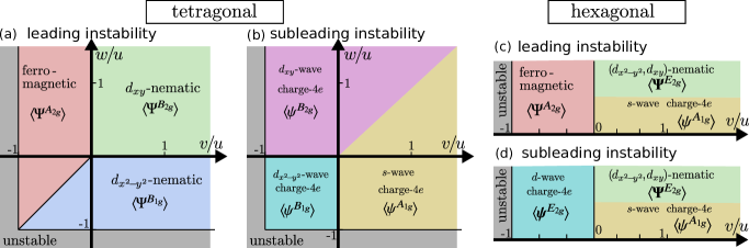
Figure 2: Large-$N$ phase diagrams for the leading and subleading vestigial-order instabilities associated with a primary two-component superconducting phase in a system with tetragonal $\mathsf{D_{4h}}$ symmetry (panels a,b) and hexagonal $\mathsf{D_{6h}}$ symmetry (panels c,d). As in the mean-field phase diagram of Fig. 1, the parameter space is that spanned by the quartic Landau coefficients of Eq. (12). The vestigial charge-$4e$ instabilities are always subleading with respect to either the vestigial nematic or the vestigial ferromagnetic instability, except in the region $v>0$ of the hexagonal phase diagram, where the vestigial $s$-wave charge-$4e$ phase and the vestigial nematic phase are degenerate.

To make the analysis more transparent, we simplify the gradient terms in Eq. (14) by setting $f_{\boldsymbol{k}}^{B_{1g}}=f_{\boldsymbol{k}}^{B_{2g}}=0$, which is equivalent to assuming that the superconducting fluctuations are isotropic in the $(k_{x},\,k_{y})$ plane. In this case, $\mathcal{G}_{k}^{0}=G_{\boldsymbol{k}}^{0}\tau^{0}\sigma^{0}$ with $G_{\boldsymbol{k}}^{0}=\left[R_{0}+\mathsf{d}_{0}(k_{x}^{2}+k_{y}^{2})+\mathsf{d}_{z}k_{z}^{2}\right]^{-1}$, and all bare susceptibilities (36)-(37) become identical:

$$\chi_{\Psi^{n}}^{(0)}=\chi_{\psi^{n}}^{(0)}=\frac{T_{0}}{V}\!\sum_{\boldsymbol{k}}\Big{(}G_{\boldsymbol{k}}^{0}\Big{)}^{2}=\frac{T_{0}}{8\pi d_{0}\sqrt{d_{z}}}\,R_{0}^{-1/2},$$ (38)

where, in the spirit of the Ginzburg-Landau expansion, we replaced $T$ by $T_{0}$. By solving Eq. (31) for $\Phi_{0}^{n}=\phi_{0}^{n}=0$, we can find how the renormalized mass $R_{0}=R_{0}\left(r_{0}\right)>0$ depends on the reduced temperature $r_{0}$. The key point is that $R_{0}$ vanishes at the (bare) superconducting transition temperature, which we denote by $r_{c}$, and increases monotonically as a function of the reduced temperature for $r_{0}>r_{c}$. Therefore, $\chi_{\Psi^{n}}^{(0)},\,\chi_{\psi^{n}}^{(0)}\rightarrow+\infty$ at the superconducting transition, which in turn implies that any negative $U_{n},u_{n}$ will cause the susceptibility of the corresponding composite order parameter to diverge before the onset of long-range superconducting order, see Eqs. (35). The reduced temperature $r_{c}^{*}$ for which the divergence takes place is given by $R_{0}\left(r_{c}^{*}\right)=R_{0}^{*}$ with

$$R_{0}^{*}\equiv T_{0}^{2}U_{n}^{2}\,\big{/}\,\big{(}16\pi^{2}d_{0}^{2}d_{z}\big{)}\,.$$ (39)

Of course, a similar expression holds for $u_{n}$. Since $R_{0}$ is a monotonically increasing function of $r_{0}$, it follows that $r_{c}^{*}>r_{c}$. In fact, $r_{c}^{*}$ can be found by substituting Eq. (39) in the self-consistent equation (31):

$$r_{c}^{*} =r_{c}+R_{0}^{*}+\frac{T_{0}U_{A_{1g}}}{2\pi\mathsf{d}_{0}\sqrt{\mathsf{d}_{z}}}\sqrt{R_{0}^{*}}$$ (40)

$$=R_{0}^{*}-\frac{T_{0}U_{A_{1g}}}{2\pi\sqrt{\mathsf{d}_{0}\mathsf{d}_{z}}}\left(\Lambda-\sqrt{R_{0}^{*}/\mathsf{d}_{0}}\right),$$ (41)

where we explicitly inserted $r_{c}=-2U_{A_{1g}}\Pi^{A_{1g}}\big{|}_{R_{0}=0}$ and the in-plane momentum cutoff $\Lambda\gg\sqrt{R_{0}^{*}/\mathsf{d}_{0}}$. Using Eqs. (39) and (41), we can gain insight into which vestigial channel has the highest critical temperature by determining the most negative interaction parameter, which we denote by $\mathtt{U}_{\mathrm{min}}\equiv\mathrm{min}\left\{U_{n},u_{n}\right\}$, since the most negative interaction parameter will correspond to the largest $R_{0}^{*}$. The issue is that the set $\left\{U_{n},u_{n}\right\}$ is not unique, as it depends on which combination of Fierz identities (18) is used to rewrite the interaction action (13) in terms of bilinears. In fact, there are infinite many $\left\{U_{n},u_{n}\right\}$ sets, which makes the analysis of determining the leading vestigial-phase instability within the large-$N$ approach intractable. To proceed, we exploit the mean-field results obtained in the previous section to impose reasonable restrictions on the $\left\{U_{n},u_{n}\right\}$ sets. We first divide the phase diagram in three regions, corresponding to each of the three mean-field superconducting ground states shown in Fig. 1(a). For each region, we only allow representations of the interaction action (13) in terms of the three bilinears that acquire non-zero values for that ground state. Moreover, we only replace a given bilinear by a combination of other bilinears according to the Fierz identities.

This procedure yields a small number of $\left\{U_{n},u_{n}\right\}$ sets. For instance, in the region of the phase diagram bounded by $v,w>0$, where the $d_{xy}$-nematic superconducting state $\langle\boldsymbol{\Delta}\rangle\sim(1,1)$ is the ground state, we find three sets $\mathcal{U}=\left\{U_{A_{1g}},\,U_{B_{2g}},\,u_{A_{1g}},\,u_{B_{2g}}\right\}$ given by:

$$\mathcal{U}_{1}= \left\{u+v,\,-w,\,w-v,\,0\right\}, \mathcal{U}_{2}= \left\{u+w,\,-v,\,0,\,v-w\right\},$$

$$\mathcal{U}_{3}= \left\{u+v+w,\,0,\,-v,\,-w\right\}.$$ (42)

They can be rewritten in a more compact form by introducing a parameter $\epsilon\in\big{\{}0,1,\frac{w}{w-v}\big{\}}$:

$$U_{A_{1g}} =u+\text{$\underline{\epsilon}$}v+\epsilon w, U_{B_{2g}} =-\text{$\underline{\epsilon}$}w-\epsilon v,$$

$$u_{A_{1g}} =\text{$\underline{\epsilon}$}(w-v), u_{B_{2g}} =\epsilon(v-w),$$ (43)

where $\text{$\underline{\epsilon}$}\equiv 1-\epsilon$. A straightforward comparison of the minimum values of the three sets in the $v,w>0$ range gives $\mathtt{U}_{\mathrm{min}}=-w\in\{U_{B_{2g}},\,u_{B_{2g}}\}$ for $w>v$ and $\mathtt{U}_{\mathrm{min}}=-v\in\{U_{B_{2g}},\,u_{A_{1g}}\}$ for $w<v$. At first sight, these results seem to suggest that the vestigial $d_{xy}$-nematic phase is degenerate with the vestigial $d_{xy}$-wave ($s$-wave) charge-$4e$ phase for $w>v$ ($w<v$). However, this is not the case because $U_{A_{1g}}$ is different in the two situations. Consider for concreteness $w>v$: while $\mathtt{U}_{\mathrm{min}}=U_{B_{2g}}=-w$ is from the set $\mathcal{U}_{1}$, for which $U_{A_{1g}}=u+v$, $\mathtt{U}_{\mathrm{min}}=u_{B_{2g}}=-w$ is from the set $\mathcal{U}_{3}$, for which $U_{A_{1g}}=u+v+w$. Now, as shown in Eq. (41), the vestigial-phase transition temperature $r_{c}^{*}$ depends on $U_{A_{1g}}$: the larger $U_{A_{1g}}$ is, the smaller $r_{c}^{*}$ is. Therefore, because $U_{A_{1g}}=u+v+w$ from set $\mathcal{U}_{3}$ is larger than $U_{A_{1g}}=u+v$ from set $\mathcal{U}_{1}$, the $d_{xy}$-nematic phase is the leading vestigial instability of the system, while the $d_{xy}$-wave charge-$4e$ phase is the sub-leading vestigial instability. The situation is analogous for $w<v$, where the $d_{xy}$-nematic phase is the leading vestigial instability and the $s$-wave charge-$4e$ phase, the subleading one. We verified the validity of this semi-quantitative argument via a direct computation of $r_{c}^{*}$.

The other regions of the phase diagram can be analyzed in a similar fashion. In the region $w<\min(0,v)$, whose mean-field ground state is the $d_{x^{2}-y^{2}}$-nematic superconducting state $\langle\boldsymbol{\Delta}\rangle\sim(1,0)$, the three relevant sets of interaction parameters are parametrized by:

$$U_{A_{1g}} \!=u+\epsilon v, U_{B_{1g}} \!=w-\text{$\underline{\epsilon}$}v, u_{A_{1g}} \!=-\epsilon v, u_{B_{2g}} \!=\text{$\underline{\epsilon}$}v,$$ (44)

where $\epsilon\in\big{\{}0,1,\frac{v-w}{v}\big{\}}$. Finally, in the $v<\min(0,w)$ region, associated with the TRSB chiral superconducting ground state $\langle\boldsymbol{\Delta}\rangle\sim(1,\mathsf{i})$, the sets of interaction parameters are given by:

$$U_{A_{1g}} \!=u+\epsilon w, U_{A_{2g}} \!=v-\text{$\underline{\epsilon}$}w, u_{B_{2g}} \!=-\epsilon w, u_{B_{1g}} \!=\text{$\underline{\epsilon}$}w,$$ (45)

with $\epsilon$ acquiring the values $\big{\{}0,1,\frac{w-v}{w}\big{\}}$. The resulting phase diagrams in Fig. 2(a)-(b) for the leading and subleading vestigial instabilities are obtained by computing the maximum transition temperature of each vestigial phase, considering the sets of interaction parameters $\left\{U_{n},u_{n}\right\}$ given above. In all cases, the real-valued composite order parameters give the leading vestigial instability and the complex-valued ones, the subleading vestigial phases.

The same analysis can be performed for the case of a two-component superconducting order parameter in a hexagonal system with point group $\mathsf{D_{6h}}$, whose mean-field phase diagram was shown in Fig. 1(b). In the $v<0$ region, for which the mean-field ground state is the chiral superconductor, there are two relevant sets of interaction parameters:

$$\left\{U_{A_{1g}}=u,\,U_{A_{2g}}=v\right\},\quad\left\{U_{A_{1g}}=u-v,\,u_{E_{2g}}=v\right\}\,.$$ (46)

Similar to the tetragonal case, in the hexagonal case the real-valued composite order parameter – the ferromagnetic $\left\langle\Psi_{A_{2g}}\right\rangle$ – wins over the complex-valued composite order parameter – the $d$-wave charge-$4e$ $\left\langle\boldsymbol{\psi}^{E_{2g}}\right\rangle$. In the phase-diagram region where the nematic superconductor is the mean-field ground state, $v>0$, there are three sets:

$$\left\{U_{A_{1g}}=u+v,\,U_{E_{2g}}=-v\right\} ,\quad\left\{U_{A_{1g}}=u+v,\,u_{A_{1g}}=-v\right\}\,,$$

$$\left\{U_{A_{1g}}=u-v,\,u_{E_{2g}}=v\right\}\,.$$ (47)

Interestingly, in this regime, there is a degeneracy between the vestigial nematic and $s$-wave charge-$4e$ states, as previously reported in Ref. (32). The resulting phase diagrams for the leading and subleading vestigial instabilities are shown in Fig. 2(c)-(d).

V Vestigial-orders phase diagram: variational approach

The inability of the large-$N$ approach to treat on an equal footing all possible composite order parameters motivates us to consider in this section an alternative method: the variational approach. Although such an approach, which has been previously employed to study real-valued composite orders (22; 11; 67), is uncontrolled, it allows one to determine the leading and subleading vestigial instabilities of the system of the action (12) in a much less biased way. The method is based on a trial action $\mathcal{S}_{0}$ that contains the variational parameters. The underlying principle relies on the general (convexity) inequality (89)

$$\langle e^{-A}\rangle \geq e^{-\langle A\rangle}.$$ (48)

To apply it to our problem, we rewrite the partition function as

$$\mathcal{Z} =\int\mathcal{D}(\boldsymbol{\Delta},\bar{\boldsymbol{\Delta}})\,e^{-\mathcal{S}}=\mathcal{Z}_{0}\,\left\langle e^{-(\mathcal{S}-\mathcal{S}_{0})}\right\rangle_{0},$$ (49)

where $\langle\mathcal{O}\rangle_{0}$ denotes the expectation value with respect to $\mathcal{S}_{0}$,

$$\langle\mathcal{O}\rangle_{0} \equiv\frac{1}{\mathcal{Z}_{0}}\int\mathcal{D}(\boldsymbol{\Delta},\bar{\boldsymbol{\Delta}})\,\,\mathcal{O}\,\,e^{-\mathcal{S}_{0}},$$ (50)

and $\mathcal{Z}_{0}\equiv\int\mathcal{D}(\boldsymbol{\Delta},\bar{\boldsymbol{\Delta}})\,e^{-\mathcal{S}_{0}}$ is the partition function of the trial action. Applying the relationship (48) to Eq. (49) leads to the inequality $F\leq F_{v}$ between the actual free energy $F=-T\log\mathcal{Z}$ and the variational free energy

$$F_{v} =-T\log\mathcal{Z}_{0}+T\langle\mathcal{S}-\mathcal{S}_{0}\rangle_{0}.$$ (51)

The remaining task is to minimize the variational free energy $F_{v}$ with respect to the variational parameters to find the optimal solution under the constraints imposed on the trial action $\mathcal{S}_{0}$. The success of this method crucially depends on the chosen ansatz for $\mathcal{S}_{0}$.

V.1 Gaussian variational ansatz

One commonly used variational ansatz is a Gaussian trial action (89; 22; 11). In this work, we employ the most general form of this ansatz by introducing a variational parameter to each of the possible bilinear combinations (7)-(8). In particular, the trial action is given by

$$\mathcal{S}_{0} =\frac{1}{2}\frac{V}{T}\sum_{k}\hat{\boldsymbol{\Delta}}_{k}^{\dagger}\,\mathcal{G}_{k}^{-1}\,\hat{\boldsymbol{\Delta}}_{k},$$ (52)

where, as in the previous section, we introduced $\hat{\boldsymbol{\Delta}}_{k}=(\boldsymbol{\Delta}_{k},\bar{\boldsymbol{\Delta}}_{-k})$, with $\boldsymbol{\Delta}_{k}=(\Delta_{1k},\Delta_{2k})$. The trial Green’s function has a similar form as Eq. (25), with $R_{0}\equiv r_{0}+\Phi^{A_{1g}}$ and $f_{\boldsymbol{k}}^{B_{1g}}=f_{\boldsymbol{k}}^{B_{2g}}=0$:

$$\mathcal{G}_{k}^{-1} =2\Big{(}\!R_{0}+\!f_{\boldsymbol{k}}^{A_{1g}}\!\Big{)}M^{A_{1g}}+2\!\!\sum_{n\in\mathbb{G}_{\mathbb{R}}}\!\!\!\Phi^{n}M^{n}+\!\!\sum_{n\in\mathbb{G}_{\mathbb{C}}}\!\!\!\left(\bar{\phi}^{n}m^{n}\!+\mathrm{H.c.}\right).$$ (53)

It is important to highlight the differences with respect to the large-$N$ approach in Sec. IV: in that case, the quantities $\Phi^{n}$, $\phi^{n}$ were auxiliary bosonic fields introduced via a Hubbard-Stratonovich transformation of the interaction action (13), which in turn depended on the representation of the latter in terms of the bilinears. As a result, only a few fields could be introduced simultaneously, which was the main limitation of the large-$N$ approach. On the other hand, in the variational approach, because $\Phi^{n}$, $\phi^{n}$ are variational parameters, we can introduce all of them simultaneously. The matrices $M^{n}$, $m^{n}$ are those defined in Eq. (26).

Having set up the Gaussian trial action (52), it is straightforward to derive the variational free energy (51); details are presented in Appendix B. We obtain the free energy density $f_{v}=F_{v}/V$ (up to an unimportant constant)

$$f_{v} =\!\frac{T}{2V}\!\!\sum_{k}\!\mathrm{tr}\log\left(\mathcal{G}_{k}^{-1}\right)+2\left[r_{0}\!-\!R_{0}\!+\!U_{A_{1g}}\Pi^{A_{1g}}\right]\!\Pi^{A_{1g}}$$

$$\quad-\!2\!\!\sum_{n\in\mathbb{G}_{\mathbb{R}}}\left[\Phi^{n}\!-\!U_{n}\Pi^{n}\right]\Pi^{n}-\!\!\!\sum_{n\in\mathbb{G}_{\mathbb{C}}}\!\!\!\left[\left(\phi^{n}\!-\!u_{n}\pi^{n}\right)\bar{\pi}^{n}\!+\mathrm{c.c.}\right],$$ (54)

where the integrals $\Pi^{n}$, $\pi^{n}$ are the same as those defined in Eq. (34); we repeat their definitions here for the sake of clarity:

$$\Pi^{n} =\frac{T}{2V}\sum_{k}\mathrm{tr}\left[\mathcal{G}_{k}M^{n}\right], \pi^{n} =\frac{T}{2V}\sum_{k}\mathrm{tr}\left[\mathcal{G}_{k}m^{n}\right].$$ (55)

In contrast to the large-$N$ approach, here the interaction parameters $\left\{U_{n},u_{n}\right\}$ are all simultaneously non-zero and unambiguously defined:

$$U_{A_{1g}} =3u+v+w, u_{A_{1g}} =u-v+w, U_{A_{2g}} =u+3v-w,$$

$$U_{B_{1g}} =u-v+3w, u_{B_{1g}} =u+v+w,$$

$$U_{B_{2g}} =u-v-w, u_{B_{2g}} =u+v-w.$$ (56)

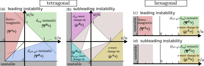
Figure 3: Variational phase diagrams for the leading and subleading vestigial-order instabilities associated with a primary two-component superconducting phase in a system with tetragonal $\mathsf{D_{4h}}$ symmetry (panels a,b) and hexagonal $\mathsf{D_{6h}}$ symmetry (panels c,d). The parameter space is that spanned by the quartic Landau coefficients of Eq. (12). The only difference with respect to the large-$N$ phase diagrams of Fig. 2 is the existence of regions where there is no vestigial instability (white region) or no subleading vestigial instability (light-gray region). Outside of these regions, the variational and large-$N$ results agree with each other.

V.2 Free-energy minimum

We now proceed to minimizing the free energy density $f_{v}$ in Eq. (54) with respect to the variational parameters, which we collectively parametrize as $X_{i}\in\left\{R_{0},\Phi^{n},\phi^{n},\bar{\phi}^{n}\right\}$, where the vector $\boldsymbol{X}$ has dimension $L=\dim\mathbb{G}_{\mathbb{R}}^{0}+2\dim\mathbb{G}_{\mathbb{C}}$. It is convenient to interpret the free energy as an implicit function of the integrals $\Pi^{n}$ and $\pi^{n}$, which are themselves functions of $X_{i}$, i.e. $\Pi^{n}\left(R_{0},\Phi^{n},\phi^{n},\bar{\phi}^{n}\right)$ and $\pi^{n}\left(R_{0},\Phi^{n},\phi^{n},\bar{\phi}^{n}\right)$. As we show in Appendix B:

$$\frac{\partial f_{v}}{\partial X_{i}}\Big{|}_{\Pi^{n},\pi^{n}} =0\,.$$ (57)

As a result, the full derivative is given by

$$\frac{df_{v}}{dX_{i}} =\!\!\!\sum_{n\in\mathbb{G}_{\mathbb{R}}^{0}}\!\!\!V_{n}\frac{\partial\Pi^{n}}{\partial X_{i}}+\!\!\sum_{n\in\mathbb{G}_{\mathbb{C}}}\!\!\Big{(}v_{n}\frac{\partial\pi^{n}}{\partial X_{i}}\!+\!\bar{v}_{n}\frac{\partial\bar{\pi}^{n}}{\partial X_{i}}\Big{)},$$ (58)

where we defined $V_{n}\equiv\frac{\partial f_{v}}{\partial\Pi^{n}}$ and $v_{n}\equiv\frac{\partial f_{v}}{\partial\pi^{n}}$. An explicit evaluation gives:

$$\!\!V_{A_{1g}} =2\left(r_{0}\!-\!R_{0}\right)\!+\!4U_{A_{1g}}\Pi^{A_{1g}},\!\!\!\!$$ (59)

$$\!\!V_{n} =-2\Phi^{n}+4U_{n}\Pi^{n}, \!\!n \in\mathbb{G}_{\mathbb{R}},$$ (60)

$$\!\!\bar{v}_{n} =-\phi^{n}+2u_{n}\pi^{n}, \!\!n \in\mathbb{G}_{\mathbb{C}}.$$ (61)

Upon introducing the $L$-dimensional vectors $\boldsymbol{\mathcal{V}}$ and $\boldsymbol{\mathcal{P}}$ with $\mathcal{V}_{i}\in\left\{V_{A_{1g}},V_{n},v^{n},\bar{v}^{n}\right\}$ and $\mathcal{P}_{i}\in\left\{\Pi^{A_{1g}},\Pi^{n},\pi^{n},\bar{\pi}^{n}\right\}$, Eqs. (58) can be expressed as a matrix equation

$$\frac{df_{v}}{dX_{i}}=\sum_{j=1}^{L}\hat{\mathcal{P}}_{ij}\,\mathcal{V}_{j},$$ (62)

with the matrix elements $\hat{\mathcal{P}}_{ij}=\frac{\partial\mathcal{P}_{j}}{\partial X_{i}}$. Because the matrix $\hat{\mathcal{P}}$ is generically non-singular, i.e. $\det\hat{\mathcal{P}}\neq 0$, the linear set of equations (62) is only solved by the trivial solution $\boldsymbol{\mathcal{V}}=0$, which is equivalent to:

$$r_{0}-R_{0} =-2U_{A_{1g}}\Pi^{A_{1g}},$$ (63)

$$\Phi^{n} =2U_{n}\Pi^{n}, \!\!n \in\mathbb{G}_{\mathbb{R}},$$ (64)

$$\phi^{n} =2u_{n}\pi^{n}, \!\!n \in\mathbb{G}_{\mathbb{C}}.$$ (65)

Recall that $\Pi^{n}$ and $\pi^{n}$ are functions of all variational fields $R_{0},\Phi^{n},\phi^{n}$. These are the self-consistent equations that determine the variational free-energy minimum. Although they have the same functional form as the large-$N$ equations (31)-(33), the key difference is that the interaction parameters are unambiguously determined by Eq. (56). We end this section by noting that the variational parameters are indeed the composite order parameters. Upon a direct computation of the bilinear expectation values, we find (see Appendix B),

$$\langle\Psi_{q=0}^{n}\rangle =2\Pi^{n}\overset{\text{(\ref{eq:var_2})}}{=}\frac{1}{U_{n}}\Phi^{n}, \langle\psi_{q=0}^{n}\rangle =2\pi^{n}\overset{\text{(\ref{eq:var_3})}}{=}\frac{1}{u_{n}}\phi^{n},$$ (66)

for $n\in\mathbb{G}_{\mathbb{R}}$ and $n\in\mathbb{G}_{\mathbb{C}}$, respectively. These expressions agree with those obtained for the large-$N$ approach, Eq. (28), upon setting $N=2$.

V.3 Hierarchy of vestigial instabilities

It is now straightforward to find the leading and subleading vestigial instabilities of the system by linearizing the self-consistent variational equations (63)-(65) in the composite fields $\Phi^{n},\phi^{n}$ independently. To leading order, the integral expansions become $\Pi^{n}\approx-\chi_{\Psi^{n}}^{(0)}\Phi^{n}$ and $\pi^{n}\approx-\chi_{\psi^{n}}^{(0)}\phi^{n}$ where the bare susceptibilities $\chi_{\Psi^{n}}^{(0)}$ and $\chi_{\psi^{n}}^{(0)}$ are defined in Eqs. (36) and (37). Substituting these expressions in the self-consistent equations leads to the following instability condition in a given channel:

$$0=1+2U_{n}\chi_{\Psi^{n}}^{(0)}\>,\quad 0=1+2u_{n}\chi_{\psi^{n}}^{(0)}\,,$$ (67)

where $\chi_{\Psi^{n}}^{(0)}=\chi_{\psi^{n}}^{(0)}$ is given by the same expression as in Eq. (38). With the instability conditions (67) and the first variational self-consistent equation (63) having the same functional structure as in the previous section, we also recover the same critical reduced temperature $r_{c}^{*}$:

$$r_{c}^{*} =R_{0}^{*}-\frac{T_{0}U_{A_{1g}}}{2\pi\sqrt{\mathsf{d}_{0}\mathsf{d}_{z}}}\left(\Lambda-\sqrt{R_{0}^{*}/\mathsf{d}_{0}}\right),$$ (68)

with $R_{0}^{*}\equiv T_{0}^{2}U_{n}^{2}\,\big{/}\,\big{(}16\pi^{2}d_{0}^{2}d_{z}\big{)}$, and similar for $u_{n}$, cf. Eq. (39).

While the expression for the critical reduced temperature (68) is the same as in the large-$N$ approach [Eq. (41)], we emphasize two important differences: (i) the interaction parameters $U_{n},u_{n}$ are unambiguously defined for all channels in Eq. (56) and (ii) the interaction parameter $U_{A_{1g}}$ is the same for all channels. Consequently, we can find out the leading and subleading vestigial instabilities by identifying the smallest and second smallest negative interaction parameters $U_{n},u_{n}$.

The resulting phase diagram for the leading vestigial instability is presented in Fig. 3(a). When compared to the large-$N$ phase diagram of Fig. 2(a), the key difference is that the variational phase diagram displays a region near the origin where no vestigial order is present [white region in Fig. 3(a)]. This result was previously found in Ref. (22) and is also consistent with the findings of Ref. (67). It can be understood by taking the $v,\,w\rightarrow 0$ limit in Eq. (56), which yields $U_{n}=u_{n}=u>0$, implying that all vestigial channels are repulsive. In contrast, none of the $U_{n}$, $u_{n}$ sets obtained in the large-$N$ approach had a contribution from $u$, which is the coefficient of the squared trivial bilinear $\left(\Psi^{A_{1g}}\right)^{2}\propto\big{(}\left|\Delta_{1}\right|^{2}+\left|\Delta_{2}\right|^{2}\big{)}^{2}$ in the original action (13). As such, $u$ penalizes large-amplitude superconducting fluctuations. In the variational approach, such an energy penalty must be overcome by the energy gain of condensing a non-trivial bilinear, which depends on combinations of $v$ and $w$. Consequently, there are threshold values for the interaction parameters $U_{n}$, $u_{n}$ below which no vestigial order emerges.

This is an important qualitative distinction between the large-$N$ and variational results: in the former case, vestigial order is a weak-coupling effect, in the sense that it emerges for any $\left|v\right|,\left|w\right|\ll u$, whereas in the latter case it is a moderate-coupling effect, as it requires $\left|v\right|,\left|w\right|\sim u$. Outside the white region of the phase diagram of Fig. 3(a), the large-$N$ and variational phase diagrams predict the same leading instabilities, which are all related to the condensation of real-valued composite order parameters. The fact that two different methods give the same results in these regions provides strong support for the emergence of vestigial phases in these parameter ranges.

The subleading vestigial instabilities can be readily obtained by computing the second smallest negative interaction parameters $U_{n}$, $u_{n}$ from Eq. (56) in the $\left(v/u,\,w/u\right)$ parameter space. Fig. 3(b) shows the resulting phase diagram. Besides the white region near the origin where no vestigial instability can take place, there is a wider light-gray region in which the system displays no subleading vestigial instability. Outside of these regions, the phase diagram agrees with that obtained in the large-$N$ approach [Fig. 2(b)], consisting of complex-valued charge-$4e$ composite order parameters with different angular momentum.

Extension of this analysis to the case of a $\mathsf{D_{6h}}$ hexagonal two-component superconductor parameterized by Eq. (2) is straightforward. In this case, the interaction parameters are given by:

$$U_{A_{1g}} =3u+v, u_{A_{1g}} =u-v, U_{A_{2g}} =u+3v,$$

$$U_{E_{2g}} =u-v, u_{E_{2g}} =u+v.$$ (69)

The phase diagrams corresponding to the leading and subleading vestigial instabilities are shown in Figs. 3(c)-(d). Similarly to the $\mathsf{D_{4h}}$ tetragonal case, there are regions of the phase diagram in which no vestigial channel is attractive (white region) or only one vestigial channel is attractive (light-gray region). Outside of these regions, the phase diagrams agree with those obtained with the large-$N$ approach, see Figs. 2(c)-(d). Interestingly, there is no subleading vestigial instability on the $v<0$ side of the phase diagram, where only the real-valued ferromagnetic composite order parameter can condense. On the $v>0$ side, the vestigial nematic instability is always degenerate with the vestigial $s$-wave charge-$4e$ instability, since $U_{E_{2g}}=u_{A_{1g}}$. Such a degeneracy, which was also present in the large-$N$ approach, has been attributed in Ref. (32) to a hidden discrete symmetry of the Ginzburg-Landau action that permutes operators in the gauge and in the lattice sectors.

V.4 Vestigial instabilities versus vestigial phases

It is important to emphasize that the phase diagrams in Figs. 2 and 3 show the parameter regimes in which there are attractive vestigial instabilities, which onset at a (reduced) temperature $r_{c}^{*}$ that is larger than the superconducting transition (reduced) temperature in the absence of vestigial order, $r_{c}$. This is a necessary but not sufficient condition to ensure the emergence of a vestigial phase preceding the primary superconducting phase. The reason is because of the feedback effect of the condensation of the composite order parameter on the superconducting fluctuations, which renormalizes the superconducting transition temperature to larger values, $\tilde{r}_{c}>r_{c}$. Thus, a vestigial phase characterized by $\left\langle\Psi^{n}\right\rangle\neq 0$ or $\left\langle\psi^{n}\right\rangle\neq 0$ while $\langle\boldsymbol{\Delta}\rangle=0$ requires $r_{c}^{*}>\tilde{r}_{c}$.

Within the variational approach, it would seem straightforward to consider a modified ansatz with $\hat{\boldsymbol{\Delta}}_{k}$ replaced by $\hat{\boldsymbol{\Delta}}_{k}-\hat{\boldsymbol{\delta}}$ in the trial action (52), where $\boldsymbol{\delta}=(\delta_{1},\delta_{2})$ denotes the superconducting variational parameter. The issue is that, even for a simple one-component superconductor, which does not have any vestigial orders, such a variational ansatz gives a first-order superconducting transition. For completeness, this analysis is presented in Appendix C; the formulas for the two-component case are given in Appendix D. The bottom line is that this unphysical result indicates that the modified trial action is not appropriate to describe the onset of superconductivity, let alone the joint onset of superconducting and composite orders. Additional work will be necessary to design an appropriate ansatz. We note that a non-mean-field first-order superconducting transition was also found in the seminal work (90), where gauge-field fluctuations were considered within a large-$N$ approach. It was later realized that this effect holds only for type-I superconductors (91; 92; 93; 94). Whether these results are related to the issues encountered in the variational approach remains to be determined.

Despite this shortcoming, one can still assess whether the condition $r_{c}^{*}>\tilde{r}_{c}$ is self-consistently satisfied by the variational equations (63)-(65), which are identical to the large-$N$ equations (31)-(33). In this formulation, $\tilde{r}_{c}$ is signaled by the vanishing of one of the eigenvalues of the Green’s function (53) [or, equivalently, (25)] evaluated at zero momentum, i.e. $\mathrm{det}\,\mathcal{G}_{k=0}^{-1}\left(\tilde{r}_{c}\right)=0$. That condition ensures that the superconducting susceptibility is divergent. When only one of the composite order parameters condenses, say $\Phi^{n}$, the latter condition is met when $R_{0}=\left|\Phi^{n}\right|$. Therefore, as long as the vestigial phase transition at $r_{c}^{*}$ is second order, i.e. $\Phi^{n}\left(r_{0}\rightarrow\left(r_{c}^{*}\right)^{-}\right)\rightarrow 0$, the vestigial instability will not trigger a simultaneous superconducting instability, implying that a vestigial phase emerges. Even if the vestigial phase transition is first-order, a vestigial phase appears as long as the jump of the composite order parameter is not too large, $\left|\Delta\Phi^{n}\right|<R_{0}^{*}$, with $R_{0}^{*}$ given by Eq. (39). The determination of whether the vestigial phase transition is second-order or first-order requires solving the non-linear equations (63)-(65). While a systematic analysis of this problem is beyond the scope of our work, important insight can be gained from previous studies of the equivalent large-$N$ equations (31)-(33).

For the tetragonal $\mathsf{D_{4h}}$ case, the large-$N$ equations for a single composite order parameter were analyzed in detail in Ref. (10) in the context of magnetically-driven nematicity and, before that, in Refs. (46; 8). The outcome of the coupled vestigial and primary transitions was found to depend not only on the quartic Landau coefficients, but also on stiffness coefficients $\mathsf{d}_{0},\,\mathsf{d}_{z}$. Essentially, systems that are more anisotropic, i.e. with $\mathsf{d}_{z}/\mathsf{d}_{0}\ll 1$, tend to display vestigial phases over wider parameter ranges.

A small modification of the model leads to more “universal” results, in the sense that they depend only on the ratio between the quartic Landau coefficients. In this modified version of the model, the anisotropic gradient term $f_{\boldsymbol{k}}^{A_{1g}}$ in Eq. (15) is replaced by an isotropic term $f_{\boldsymbol{k}}^{A_{1g}}=\mathsf{d}_{0}\boldsymbol{k}^{2}$, but the dimensionality of the system $d$ is allowed to assume fractional values $2\leq d\leq 3$. As shown in Ref. (10) (see also Ref. (46)), for a given vestigial instability with attractive effective interaction $U_{n}<0$ or $u_{n}<0$, there are three different regimes for the coupled vestigial and superconducting phase transitions, which we denote here as: (i) type-I split transitions, in which case the vestigial and superconducting instabilities are split and second-order; (i) type-II split transitions, in which case the vestigial and superconducting instabilities are split but one of them is first-order; (iii) simultaneous transition, in which case there is a single first-order vestigial plus superconducting transition. The system’s regime depends only on the ratio $\left|U_{n}\right|/U_{A_{1g}}$ and the dimensionality $d$ according to (10):

$$\frac{\left|U_{n}\right|}{U_{A_{1g}}} <3-d, \textrm{type-I}\;\textrm{split},$$ (70)

$$3-d<\frac{\left|U_{n}\right|}{U_{A_{1g}}} <\frac{6-2d}{6-d}, \textrm{type-II\;{split}},$$ (71)

$$\frac{\left|U_{n}\right|}{U_{A_{1g}}} >\frac{6-2d}{6-d}, \textrm{simultaneous}\;\textrm{transitions}.$$ (72)

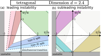
Figure 4: Variational phase diagrams of Fig. 3 for the tetragonal $\mathsf{D_{4h}}$ case with the phase boundaries $\left|U_{n}\right|/U_{A_{1g}}=3-d$ (dotted line) and $\left|U_{n}\right|/U_{A_{1g}}=(6-2d)/(6-d)$ (dashed line) that determine the three different regimes for the coupled vestigial and superconducing transitions (see main text): two split second-order transitions (labeled type-I split); two split transitions with one of them first-order (labeled type-II split); one simultaneous first-order transition. For concreteness, here we set $d=2.4$.

Of course, similar expressions hold for $\left|u_{n}\right|/U_{A_{1g}}$. The key point is that a vestigial phase only exists in the type-I split and type-II split regimes. In Fig. 4, we include the phase boundaries set by Eqs. (70)-(72) separating these three regimes in the variational phase diagram of Fig. 3, for the case $d=2.4$. Clearly, there is a wide region in parameter space where the vestigial instability leads to a vestigial phase. Note that, upon increasing the dimensionality $d$, the lines move closer to the origin, which decreases the area of the phase diagram where vestigial phases exist. In the fully isotropic case $d=3$, vestigial phases are absent, as noted in Refs. (46; 10).

For the hexagonal $\mathsf{D_{6h}}$ case, the vestigial nematic transition is that of a 3-state Potts-model, which is first-order above its upper critical dimension $d_{\mathrm{upper}}\lesssim 3$. This problem was analyzed in Ref. (25) for a system with lower trigonal point-group symmetry $\mathsf{D_{3d}}$, which has the additional stiffness coefficient $\mathsf{d}_{3}$ discussed below Eq. (14). A wide regime where vestigial nematic order emerges was reported for a sufficiently anisotropic system. Note also that even in the dark-gray regions of the phase diagrams in Figs. 2 and 3, where the bare superconducting transition is itself first-order, it is in principle possible for a vestigial phase to be stabilized. However, our formalism does not allow us to access these regions.

More broadly, the fact that there is more than one attractive vestigial channel suggests that it is in principle possible for the system to have sequential vestigal instabilities, giving rise to a cascade of vestigial phases. The aforementioned issues with the modified Gaussian variational ansatz that includes a non-zero superconducting order parameter make a quantitative analysis challenging. On a qualitative level, it is interesting to note that, in the cases studied here, there is always a symmetry-allowed trilinear coupling between one real-valued and two complex-valued bilinears. Specifically, for the $\mathsf{D_{4h}}$ case, there are three such trilinear couplings with coefficients $\tilde{\lambda}_{i}$,

$$\tilde{\mathcal{S}}_{1} =\tilde{\lambda}_{1}\int_{\mathsf{x}}\Psi^{B_{1g}}\left(\psi^{A_{1g}}\bar{\psi}^{B_{1g}}+\bar{\psi}^{A_{1g}}\psi^{B_{1g}}\right),$$ (73)

$$\tilde{\mathcal{S}}_{2} =\tilde{\lambda}_{2}\int_{\mathsf{x}}\Psi^{B_{2g}}\left(\psi^{A_{1g}}\bar{\psi}^{B_{2g}}+\bar{\psi}^{A_{1g}}\psi^{B_{2g}}\right),$$ (74)

$$\tilde{\mathcal{S}}_{3} =\tilde{\lambda}_{3}\int_{\mathsf{x}}\Psi^{A_{2g}}\,\mathsf{i}\left(\bar{\psi}^{B_{2g}}\psi^{B_{1g}}-\bar{\psi}^{B_{1g}}\psi^{B_{2g}}\right),$$ (75)

whereas for the $\mathsf{D_{6h}}$ case there is only one:

$$\tilde{\mathcal{S}}_{1} =\tilde{\lambda}_{1}\int_{\mathsf{x}}\boldsymbol{\Psi}^{E_{2g}}\cdot\left(\psi^{A_{1g}}\bar{\boldsymbol{\psi}}^{E_{2g}}+\bar{\psi}^{A_{1g}}\boldsymbol{\psi}^{E_{2g}}\right).$$ (76)

Because of these couplings, if the complex-valued composite order parameter associated with the subleading instability condenses inside the leading vestigial phase, it will necessarily trigger a non-zero complex-valued composite order parameter associated with the third channel. However, as Fig. 3(b) or Eq. (69) shows, this third channel is always repulsive. Due to this parasitic effect, the system would incur an energy penalty if the subleading attractive complex-valued order parameter were to condense inside the primary vestigial phase.

VI Discussion and conclusions

In summary, we employed a group-theoretical formalism to classify and investigate all possible vestigial orders that emerge in two-component superconductors in systems with fourfold or sixfold/threefold rotational symmetry. Our focus was to treat on an equal footing the widely investigated real-valued ferromagnetic or nematic bilinears and the little-explored complex-valued bilinears that describe $s$-wave, $d_{x^{2}-y^{2}}$-wave, and $d_{xy}$-wave charge-$4e$ condensates. The large-$N$ and variational calculations that we performed reveal that the real-valued vestigial-order instabilities are always the leading ones, although the complex-valued vestigial-order channels are attractive over wide regions of the parameter space spanned by the quartic coefficients of the phenomenological Ginzburg-Landau action. Only in the particular case of a hexagonal system with quartic coefficient $v>0$ we found degenerate nematic and charge-$4e$ vestigial instabilities, as first pointed out in Ref. (32). In all other cases, the charge-$4e$ composite order was found to be subleading with respect to the ferromagnetic or nematic composite orders.

Our systematic comparison between the controlled large-$N$ method with the uncontrolled variational method revealed important caveats of both approaches in their ability to describe vestigial phases. The large-$N$ method does not offer a way to treat on an equal footing all possible real-valued and complex-valued bilinears, whereas the variational method faces difficulties to account for the instability of the primary superconducting order parameter. Notwithstanding these shortcomings, we found wide regions in the parameter-space where the hierarchy of instabilities obtained from both methods agreed with each other, giving us confidence on the reliability of these findings. One important qualitative difference between the two methods is that, in the large-$N$ approach, the emergence of vestigial orders is a weak-coupling effect, in that the Landau coefficients of the non-trivial squared bilinears can be much smaller than the coefficient of the trivial squared bilinear. On the other hand, in the variational approach, it is a moderate-coupling effect, in that the non-trivial coefficients need to be comparable to the trivial coefficient in order for the vestigial channels to become attractive. This difference stems from the distinct ways in which large-amplitude fluctuations are energetically penalized in each scenario. Because both methods have intrinsic limitations – the physical $N$ in our problem is not large and the variational action ansatz is arbitrary – it will be interesting to exactly solve this model via Monte Carlo simulations to elucidate the validity of each approach. Previous Monte Carlo calculations on a related Ginzburg-Landau model seem to be qualitatively consistent with the large-$N$ results (95).

We note that, by setting $f_{\boldsymbol{k}}^{B_{1g}}=f_{\boldsymbol{k}}^{B_{2g}}=0$ in Eq. (14), the phase diagrams obtained in this work neglected the in-plane anisotropic gradient terms that are allowed in the Ginzburg-Landau action. Inclusion of these terms is expected to cause minor changes in the phase boundaries. The most important impact would be on the degeneracy between the nematic and charge-$4e$ orders in the $v>0$ region of the phase diagram of the hexagonal system. Interestingly, in the large-$N$ approach of Ref. (32), these additional gradient terms were shown to remove the degeneracy by actually favoring the charge-$4e$ vestigial phase. A more important effect not considered here, which has been little explored in the broader context of superconducting vestigial orders, is the coupling to the electromagnetic gauge fields. These should be particularly relevant for nearly-2D systems, where phase fluctuations can play a more important role than amplitude fluctuations. A recent work showed that the phase boundaries of the mean-field phase diagrams shown in Fig. 1 are fundamentally changed when corrections due to electromagnetic fluctuations are included (96). Their impact on the onset of vestigial phases deserve further investigations.

From a broader theoretical standpoint, our work reveals that there is a larger and relatively unexplored landscape of vestigial orders that can potentially be realized in systems whose symmetry group $\mathcal{G}=\mathcal{G}_{\mathrm{int}}\otimes\mathcal{G}_{s}$ is the product of a space group and an internal group. Here, we focused on the complex-valued charge-$4e$ bilinears of superconductors, which transform non-trivially under the internal group $\mathcal{G}_{\mathrm{int}}=U(1)$. In magnetic systems, with internal group $\mathcal{G}_{\mathrm{int}}=SU(2)$, the bilinears that transform non-trivially would be vector and tensorial composite order parameters. A well-known example of the latter is the spin-nematic order parameter, which has been proposed to be realized in certain frustrated magnets (97; 98). While other types of vestigial tensorial spin orders were briefly discussed in Ref. (6), a systematic investigation has not been performed. Of course, the independent classification of magnetic bilinears in terms of IRs of $\mathcal{G}_{\mathrm{int}}=SU(2)$ and $\mathcal{G}_{s}$ is only meaningful if the spin-orbit coupling is weak, which may constrain their realization in actual materials. These considerations for non-trivial vestigial phases are also relevant for systems with emergent continuous symmetries – such as twisted bilayer graphene, which under certain conditions is described by a model with emergent spin-valley $SU(4)$ or $U(4)\otimes U(4)$ symmetry (99; 100; 101; 102).

Because vestigial phases are fluctuation-driven phenomena, they are most likely to be observed in low-dimensional and/or unconventional superconductors, since the fluctuation regime of conventional BCS superconductors is very narrow. In this regard, several materials have been recently reported or proposed to be multi-component nematic or chiral unconventional superconductors, making them natural candidates to search for vestigial orders. This is the case for the doped topological insulator $A_{\mathrm{x}}\mathrm{Bi_{2}Se_{3}}$, with $A=\mathrm{Cu},\,\mathrm{Nb},\,\mathrm{Sr}$, which has a nematic superconducting ground state (73; 74; 75; 76; 77; 25). Recent experiments have found strong evidence for a vestigial nematic order preceding the superconducting phase (103; 104). Twisted bilayer graphene has also been shown to display nematic superconductivity (14), and hints of a possible vestigial nematic phase were observed in anisotropic transport measurements. $\mathrm{CaSn_{3}}$ (105) and few-layer $\mathrm{NbSe_{2}}$ (106; 107) are other examples of materials whose pairing states are accompanied by broken lattice rotational symmetry; however, at least in the latter, the data does not favor an interpretation in terms of a multi-component superconductor. The heavy-fermion material $\mathrm{UPt_{3}}$ is a well-established candidate for chiral two-component $f$-wave superconductivity (78; 79; 80), which could host vestigial orders as well. The same holds for other compounds where time-reversal symmetry-breaking (TRSB) superconductivity has been reported, most notably $\mathrm{Sr_{2}RuO_{4}}$ (68; 69), $\mathrm{URu_{2}Si_{2}}$ (70; 71; 72), pressurized $\mathrm{KV_{3}Sb_{5}}$ (108), and 4Hb-$\mathrm{TaS_{2}}$ (109) (for a more comprehensive list, see Ref. (110)). In these cases, however, it remains unsettled whether the observed TRSB arises from a symmetry-enforced two-component superconducting order parameter. In 4Hb-$\mathrm{TaS_{2}}$, recent Little-Parks (111) and critical field (112) experiments provide strong support for such a scenario. On the other hand, in $\mathrm{Sr_{2}RuO_{4}}$, which has been recently proposed to be a two-component singlet superconductor (113; 114), the observation of nodal quasi-particles and the lack of specific heat signatures across the second superconducting transition have been interpreted in terms of an accidental degeneracy between two one-component superconductors transforming as different IRs (115; 116). It is important to emphasize that vestigial phases can emerge even in cases where the degeneracy between two superconducting orders is not symmetry-enforced, but accidental, as discussed in Ref. (29). One superconductor where this might be the case is $\mathrm{UTe_{2}}$, which was also reported to spontaneously break time-reversal symmetry (117). Since its orthorhombic $\mathsf{D_{2h}}$ point group does not support two-dimensional IRs, a TRSB superconducting state would require two nearly degenerate states; however, whether $\mathrm{UTe_{2}}$ is a single or two-component superconductor remains unsettled (118). Signatures consistent with a vestigial TRSB order have been recently reported in K-doped $\mathrm{BaFe_{2}As_{2}}$ (119), whose ground state has been proposed to be a TRSB $s+\mathsf{i}s$ state (120; 121).

Overall, our work significantly expands the class of systems where the elusive charge-$4e$ condensates may be realized (56; 57; 58; 59; 60; 61; 15; 62; 54; 16; 63; 64; 30; 65; 32; 33; 55; 66). Experimentally, recent magnetoresistance oscillation data in the kagome superconductor $\mathrm{CsV_{3}Sb_{5}}$ have been interpreted as signatures of charge-$4e$ and charge-$6e$ states above the onset of charge-$2e$ order (122). Theoretically, it has been previously shown that pair-density waves (15; 16), coupled $U(1)\times U(1)$ superconductors (54), and hexagonal nematic superconductors (32; 33) are good candidates to display vestigial $s$-wave charge-$4e$ order. Our results reveal that, in fact, there are normal-state instabilities in the charge-$4e$ channel in any two-component superconductor. Interestingly, this instability is not restricted to the $s$-wave channel, but includes also exotic $d$-wave charge-$4e$ states, whose properties deserve further theoretical investigations. The main issue is that, except for the case of a hexagonal nematic superconductor, the various vestigial charge-$4e$ instabilities found here are subleading with respect to the vestigial nematic or ferromagnetic instabilities. One way in which this hierarchy of vestigial instabilities can be reversed is via disorder, as previously discussed in Ref. (32) in the context of hexagonal nematic superconductors. Quite generally, the type of disorder that is most detrimental for a given ordered state is a random distribution of conjugate fields of the corresponding order parameter – also known as “random-field” disorder (123). Charge-$4e$ order parameters are generally protected from random-field type of disorder, as their conjugate fields are not present in crystals or devices. In contrast, random strain and, to a lesser extent, diluted magnetic impurities, are present in many realistic settings, acting as random-field disorder for the nematic and ferromagnetic order parameters, respectively. The ability to control these types of disorder could enable the stabilization of the subleading vestigial charge-$4e$ states. Even in a perfectly clean system, the presence of a subleading attractive charge-$4e$ instability should be manifested in the collective excitations of the leading vestigial phase, opening another route to access this elusive state of matter.

Appendix A Group-theoretical formalism

In this Appendix, we present the group-theoretical framework that yields the results presented in Sec. II of the main text for the bilinears of the two-component superconducting order parameters in Eqs. (1)-(2), which live in the product group $\mathcal{G}=U(1)\otimes\mathcal{G}_{p}$, with $\mathcal{G}_{p}=\mathsf{D_{4h}}$ or $\mathcal{G}_{p}=\mathsf{D_{6h}}$. The approach is the same as in Ref. (6), but generalized to include complex-valued bilinears.

We start by studying a standard one-component superconductor with order parameter $\Delta$. All bilinears are trivial under the operations of the point group, since the product of two one-dimensional IRs always yields the trivial IR $A_{1g}$. Thus, it is enough to focus on the transformation properties of the unitary group $\mathcal{G}=U(1)$, whose IRs we denote by $\Gamma_{m}^{U}$ , with $m=\{0,\pm 1,\pm 2,\dots\}$. If the order parameter $\Delta$ transforms according to the IR $\Gamma_{+1}^{U}$, then its complex conjugate $\bar{\Delta}$ transforms as $\Gamma_{-1}^{U}$. Thus, the reasonable representation of the order parameter is given through the “Nambu” vector $\hat{\boldsymbol{\Delta}}=(\Delta,\bar{\Delta})$, which transforms according to the two-dimensional representation $\Gamma_{\Delta}=\Gamma_{+1}^{U}\oplus\Gamma_{-1}^{U}$. This notation becomes more transparent if we consider the $U(1)$ symmetry operations as rotations in the complex plane:

$$\left(\begin{array}[]{c}\Re\Delta^{\prime}\\ \Im\Delta^{\prime}\end{array}\right) =\left(\begin{array}[]{cc}\cos\varphi&-\sin\varphi\\ \sin\varphi&\cos\varphi\end{array}\right)\left(\begin{array}[]{c}\Re\Delta\\ \Im\Delta\end{array}\right).$$ (83)

The transformation relation (83) can be (block-) diagonalized upon application of the unitary matrix

$$U =\frac{1}{\sqrt{2}}\left(\begin{array}[]{cc}1&1\\ -\mathsf{i}&\mathsf{i}\end{array}\right),$$

which leads to the relation

$$\hat{\boldsymbol{\Delta}}^{\prime} =\mathcal{R}_{\Delta}(\varphi)\hat{\boldsymbol{\Delta}}.$$ (84)

Here, $\mathcal{R}_{\Delta}(\varphi)=\mathcal{R}_{+1}(\varphi)\oplus\mathcal{R}_{-1}(\varphi)$ and $\mathcal{R}_{m}(\varphi)=e^{\mathsf{i}m\varphi}$ is the transformation matrix associated with the IR $\Gamma_{m}^{U}$, see Table 2. The transformation relation (84) demonstrates that the rotation of the two real components $(\Re\Delta,\Im\Delta)$ in the complex plane is properly described by means of the Nambu vector $\hat{\boldsymbol{\Delta}}$ transforming as $\Gamma_{\Delta}$.

Next, we consider bilinear combinations of $\hat{\boldsymbol{\Delta}}$. From the decomposition of the product representation (4), $\Gamma_{\Delta}\otimes\Gamma_{\Delta}=2\Gamma_{0}^{U}\oplus\left(\Gamma_{+2}^{U}\oplus\Gamma_{-2}^{U}\right)$, there are two bilinears associated with the trivial sector and two with the $m=\pm 2$ (i.e. charge-$4e$) sector. The bilinears can be written as

$$C^{(m)} =\frac{1}{2}\hat{\boldsymbol{\Delta}}^{T}\lambda^{m}\hat{\boldsymbol{\Delta}},$$ (85)

with the $2\times 2$ matrices $\lambda^{m}$ acting in Nambu space. These matrices $\lambda^{m}$ are defined implicitly through the transformation condition

$$\mathcal{R}_{\Delta}^{T}(\varphi)\lambda^{m}\mathcal{R}_{\Delta}(\varphi) =\mathcal{R}_{m}(\varphi)\lambda^{m}, \forall\varphi \in[0,2\pi).$$ (86)

Applying this condition, we find the matrices shown in Table 2. Inserting these matrices into Eq. (85), we obtain the $N_{\Gamma_{\Delta}}=3$ bilinear components

$$C^{(0)} =|\Delta|^{2}, C^{(+2)} =\Delta^{2}, C^{(-2)} =\bar{\Delta}^{2},$$ (87)

transforming according to $\Gamma_{0}^{U}$, $\Gamma_{+2}^{U}$, and $\Gamma_{-2}^{U}$, respectively. While the antisymmetric matrix associated with the trivial IR $\Gamma_{0}^{U}\big{|}_{a}$ yields a vanishing bilinear (85) in the present case, it plays a role when multiple groups are involved, as it can be paired with another antisymmetric matrix.

$U(1)$	$E$	$\mathcal{R}_{m}(\varphi)$
$\Gamma_{m}^{U}$	$1$	$e^{\mathsf{i}m\varphi}$

    $U(1)$ $\lambda^{m}$ $\Gamma_{0}^{U}\big{|}_{s}$ $\sigma^{x}$ $\Gamma_{0}^{U}\big{|}_{a}$ $-\mathsf{i}\,\sigma^{y}$ $\Gamma_{+2}^{U}$ $\sigma^{0}+\sigma^{z}$ $\Gamma_{-2}^{U}$ $\sigma^{0}-\sigma^{z}$ $\mathsf{D_{4h}}$ $\tau^{n,l}$ $A_{1g}$ $\tau^{0}$ $A_{2g}$ $\tau^{y}$ $B_{1g}$ $\tau^{z}$ $B_{2g}$ $\tau^{x}$ $\mathsf{D_{6h}}$ $\tau^{n,l}$ $A_{1g}$ $\tau^{0}$ $A_{2g}$ $\tau^{y}$ $E_{2g}$ $(\tau^{z},-\tau^{x})$

Table 2: (left) The character table of the unitary group $U(1)$ and its IRs $\Gamma_{m}^{U}$, $m\in\mathbb{Z}$. (middle-left to right) Matrices associated with the bilinear decomposition in the cases of the one-component SC [Eqs. (86) and (4)] and of two-component real-valued order parameters transforming as two-dimensional IRs of the point groups $\mathsf{D_{4h}}$ and $\mathsf{D_{6h}}$ [Eqs. (89), (5) and (6)].

We now proceed by constructing the bilinears of a real-valued two-component order parameter $\boldsymbol{\eta}=(\eta_{1},\eta_{2})$ that transforms according to the IRs $E_{g}$ and $E_{u}$ of the point group $\mathcal{G}_{p}=\mathsf{D_{4h}}$ or the IRs $E_{1g}$, $E_{2g}$, $E_{1u}$, and $E_{2u}$ of the point group $\mathcal{G}_{p}=\mathsf{D_{6h}}$. The bilinears are defined as

$$C^{n,l} =\boldsymbol{\eta}^{T}\tau^{n,l}\boldsymbol{\eta},$$ (88)

where $n$ denotes the IR within the product decompositions in Eqs. (5) and (6) (see also Table 2) and $l=1,\dots,\dim n$. Like in the $U(1)$ case, the associated $2\times 2$ matrices $\tau^{n,l}$ are defined implicitly through the transformation condition

$$\mathcal{R}_{E_{g}}^{T}(g)\tau^{n,l}\mathcal{R}_{E_{g}}(g) =\sum_{l^{\prime}}\mathcal{R}_{n}(g)_{ll^{\prime}}\tau^{n,l^{\prime}}, \forall g \in\mathcal{G}_{p},$$ (89)

where $\mathcal{R}_{n}(g)$ denotes the transformation matrix for the group element $g$ within the IR $n$. Solving this equation gives the matrices shown in Table 2. Consequently, the bilinears (88) become

$$\mathsf{D_{4h}} : \!\!\!\!C^{A_{1g}} =\eta_{1}^{2}+\eta_{2}^{2}, \!\!\!C^{B_{1g}} =\eta_{1}^{2}-\eta_{2}^{2},\;\;C^{B_{2g}}=2\eta_{1}\eta_{2},$$ (90)

$$\mathsf{D_{6h}} : \!\!\!\!C^{A_{1g}} =\eta_{1}^{2}+\eta_{2}^{2}, \!\!\!\boldsymbol{C}^{E_{2g}} =\big{(}\eta_{1}^{2}-\eta_{2}^{2},-2\eta_{1}\eta_{2}\big{)}.$$ (91)

Note that the antisymmetric matrix associated with the $A_{2g}$ bilinear yields zero, i.e. $C^{A_{2g}}=0$.

We are now in position to derive the bilinears of the two-component superconducting order parameter $\boldsymbol{\Delta}=(\Delta_{1},\Delta_{2})$ of Eqs. (1)-(2) by combining the bilinear decompositions obtained for the groups $U(1)$ and $\mathsf{\mathcal{G}_{p}}$ studied above. Let us start with the $\mathcal{G}_{p}=\mathsf{D_{4h}}$ case; as explained before, the superconducting order parameter is given in the Nambu representation by $\hat{\boldsymbol{\Delta}}=(\boldsymbol{\Delta},\bar{\boldsymbol{\Delta}})^{T}$, where the four-component “vector” $\hat{\boldsymbol{\Delta}}$ transforms as the representation $\Gamma=\Gamma_{\Delta}\otimes E_{i}$ of the symmetry group $\mathcal{G}=U(1)\otimes\mathsf{D_{4h}}$. The bilinears are given by

$$C^{(m),n} =\frac{1}{2}\hat{\boldsymbol{\Delta}}^{T}\lambda^{m}\tau^{n}\hat{\boldsymbol{\Delta}},$$ (92)

where $\lambda^{m}$ and $\tau^{n}$ act on the Nambu (i.e. gauge) and the $E_{i}$ (i.e. lattice) sectors, respectively. Since these matrices are defined implicitly by the conditions (86) and (89), they are the same matrices shown before in Table 2. Thus, to identify the bilinear components $C^{(m),n}$, all we need to do is construct a “multiplication table” according to the bilinear decompositions in the two sectors:

$$\Gamma\otimes\Gamma =\left(\Gamma_{\Delta}\otimes\Gamma_{\Delta}\right)\otimes\left(E_{i}\otimes E_{i}\right)$$

$$=\big{(}2\Gamma_{0}^{U}\oplus\Gamma_{+2}^{U}\oplus\Gamma_{-2}^{U}\big{)}\otimes\left(A_{1g}\oplus A_{2g}\oplus B_{1g}\oplus B_{2g}\right).$$

Such a multiplication table is given in Table 1 of the main text. Out of the $16$ possible bilinear combinations, only $N_{\Gamma}=10$ components are non-zero. Inserting the matrices into Eq. (92) gives

$$\Psi^{A_{1g}} \!=|\Delta_{1}|^{2}+|\Delta_{2}|^{2}, \!\!\psi^{\!A_{1g}} \!=\Delta_{1}^{2}+\Delta_{2}^{2}, \!\!\Psi^{A_{2g}} \!=\mathsf{i}\bar{\Delta}_{2}\Delta_{1}\!-\mathsf{i}\bar{\Delta}_{1}\Delta_{2},$$

$$\Psi^{B_{1g}} \!=|\Delta_{1}|^{2}-|\Delta_{2}|^{2}, \!\!\psi^{\!B_{1g}} \!=\Delta_{1}^{2}-\Delta_{2}^{2},$$

$$\Psi^{B_{2g}} \!=\bar{\Delta}_{1}\Delta_{2}\!+\bar{\Delta}_{2}\Delta_{1}, \!\!\psi^{\!B_{2g}} \!=2\Delta_{1}\Delta_{2},$$ (93)

where we have employed the same notation as in the main text, i.e. real-valued bilinears ($m=0$) are labeled as $\Psi^{n}$ and complex-valued ones ($m=\pm 2$), as $(\psi^{n},\bar{\psi}^{n})$. The expressions (93) are identical to those in Eq. (9) of the main text. Alternatively, one can exploit the property $\hat{\boldsymbol{\Delta}}^{T}=\hat{\boldsymbol{\Delta}}^{\dagger}\sigma^{x}$ to rewrite the bilinears (92) as

$$\Psi^{n} =\hat{\boldsymbol{\Delta}}^{\dagger}M^{n}\hat{\boldsymbol{\Delta}}, \psi^{n} =\hat{\boldsymbol{\Delta}}^{\dagger}m^{n}\hat{\boldsymbol{\Delta}}.$$ (94)

Here, the matrices $M^{n}$, $m^{n}$ are defined as:

$$M^{A_{1g}} =\tau^{0}\sigma^{0}/2, m^{A_{1g}} =\tau^{0}\sigma^{-}, M^{A_{2g}} =\tau^{y}\sigma^{z}/2,$$

$$M^{B_{1g}} =\tau^{z}\sigma^{0}/2, m^{B_{1g}} =\tau^{z}\sigma^{-},$$

$$M^{B_{2g}} =\tau^{x}\sigma^{0}/2, m^{B_{2g}} =\tau^{x}\sigma^{-},$$ (95)

with $\sigma^{\pm}=(\sigma^{x}\pm\mathsf{i}\sigma^{y})/2$, which gives Eq. (26) in the main text. This is the notation used in Secs. IV and V of the main text. The case $\mathcal{G}_{p}=\mathsf{D_{6h}}$ can be treated in the same way. The only change is that the bilinears denoted by $\Psi^{B_{1g}}$, $\Psi^{B_{2g}}$ and $\psi^{B_{1g}}$, $\psi^{B_{2g}}$, which in the $\mathsf{D_{4h}}$ case transform as two separate one-dimensional IRs, combine to transform as the same two-dimensional IR, $\boldsymbol{\Psi}^{E_{2g}}=(\Psi^{B_{1g}},-\Psi^{B_{2g}})$ and $\boldsymbol{\psi}^{E_{2g}}=(\psi^{B_{1g}},-\psi^{B_{2g}})$. All bilinears of the $\mathsf{D_{6h}}$ case are also displayed in Table 1.

Appendix B Derivation of the Variational free energy

In this Appendix, we derive the expression for the variational free energy (54) and the corresponding self-consistent equations presented in Sec. V. The Gaussian trial action (52) is given by

$$\mathcal{S}_{0} =\frac{1}{2}\frac{V}{T}\sum_{k}\hat{\boldsymbol{\Delta}}_{k}^{\dagger}\,\mathcal{G}_{k}^{-1}\,\hat{\boldsymbol{\Delta}}_{k}\,,$$ (96)

with the inverse Green’s function $\mathcal{G}_{k}^{-1}$ introduced in Eq. (53) and repeated here for convenience:

$$\mathcal{G}_{k}^{-1} =2\Big{(}\!R_{0}+\!f_{\boldsymbol{k}}^{A_{1g}}\!\Big{)}M^{A_{1g}}+2\!\!\sum_{n\in\mathbb{G}_{\mathbb{R}}}\!\!\!\Phi^{n}M^{n}+\!\!\sum_{n\in\mathbb{G}_{\mathbb{C}}}\!\!\!\left(\bar{\phi}^{n}m^{n}\!+\mathrm{H.c.}\right).$$ (97)

Our goal is to compute the variational free energy (51), or equivalently, the variational free energy density:

$$f_{v}=\frac{F_{v}}{V}=-\frac{T}{V}\,\log\mathcal{Z}_{0}+\frac{T}{V}\left\langle\mathcal{S}-\mathcal{S}_{0}\right\rangle_{0}\,,$$ (98)

where the expectation values are taken with respect to the trial action $\mathcal{S}_{0}$ as introduced in Eq. (50), and $\mathcal{Z}_{0}\equiv\int\mathcal{D}(\boldsymbol{\Delta},\bar{\boldsymbol{\Delta}})\,e^{-\mathcal{S}_{0}}$. For completeness, we also reproduce the initial action $\mathcal{S}=\mathcal{S}^{(2)}+\mathcal{S}^{\mathrm{int}}$, Eq. (12), with the second- and fourth-order contributions:

$$\mathcal{S}^{(2)} =\frac{V}{T}\sum_{k}\hat{\boldsymbol{\Delta}}_{k}^{\dagger}\left(f_{\boldsymbol{k}}^{A_{1g}}+r_{0}\right)M^{A_{1g}}\hat{\boldsymbol{\Delta}}_{k},$$ (99)

$$\mathcal{S}^{\mathrm{int}} =\int_{\mathsf{x}}\Big{[}u\,\big{(}\Psi^{A_{1g}}\big{)}^{2}+v\,\big{(}\Psi^{A_{2g}}\big{)}^{2}+w\,\big{(}\Psi^{B_{1g}}\big{)}^{2}\Big{]},$$ (100)

where, in line with the ansatz (97), the non-trivial fluctuations $f_{\boldsymbol{k}}^{B_{1g}}=f_{\boldsymbol{k}}^{B_{2g}}=0$ have been set to zero. In the following, we compute separately the three contributions to the free energy density (98):

$$f_{v}^{(0)} =-\frac{T}{V}\,\log\mathcal{Z}_{0}, f_{v}^{(2)} =\frac{T}{V}\left\langle\mathcal{S}^{(2)}-\mathcal{S}_{0}\right\rangle_{0},$$

$$f_{v}^{(4)} =\frac{T}{V}\left\langle\mathcal{S}^{\mathrm{int}}\right\rangle_{0}.$$ (101)

Before doing so, we emphasize the absence of the ambiguity caused by the Fierz identities (18) which posed a problem to the large-$N$ method. The interaction action (100) only enters into the variational free energy through the contribution $f_{v}^{(4)}$. Here, however, because the expectation value is a linear map, the Fierz relations are still intact. More explicitly, if we would choose the interaction representation as in Eq. (17), we would compute

$$f_{v}^{(4)} =\frac{T}{V}\int_{\mathsf{x}}\Big{[}\left(u+w\right)\left\langle\big{(}\Psi^{A_{1g}}\big{)}^{2}\right\rangle_{0}+\left(v-w\right)\left\langle\big{(}\Psi^{A_{2g}}\big{)}^{2}\right\rangle_{0}$$

$$\qquad\quad-w\,\left\langle\big{(}\Psi^{B_{2g}}\big{)}^{2}\right\rangle_{0}\Big{]}.$$ (102)

Meanwhile, the insertion of the Fierz relation

$$\big{(}\Psi^{B_{2g}}\big{)}^{2}=\big{(}\Psi^{A_{1g}}\big{)}^{2}-\big{(}\Psi^{B_{1g}}\big{)}^{2}-\big{(}\Psi^{A_{2g}}\big{)}^{2},$$ (103)

reduces the expression (102) to the free energy contribution that follows from the representation (100). The same is true for any other interaction representation. In other words, all interaction representations lead to the same result, and, for convenience, we choose to work with the representation (100).

The evaluation of the Gaussian integral in the partition function gives

$$\mathcal{Z}_{0} =\prod_{k}\,\Big{[}\det\big{(}VT\mathcal{G}_{k}^{-1}\big{)}\Big{]}^{-1/2},$$ (104)

and thus, the first free energy contribution becomes

$$f_{v}^{(0)} =\frac{T}{2V}\sum_{k}\mathrm{tr}\,\log\left(\mathcal{G}_{k}^{-1}\right).$$ (105)

Here, we dropped an unimportant constant and used the identity $\log\,\det\left(\mathcal{G}_{k}^{-1}\right)=\mathrm{tr}\,\log\left(\mathcal{G}_{k}^{-1}\right)$.

To derive the second- and fourth-order contributions in (101), it remains to evaluate the expectation values

$$\left\langle\!\Psi_{q=0}^{n}\right\rangle_{0} \!=\!\sum_{k}\!\left\langle\hat{\boldsymbol{\Delta}}_{k}^{\dagger}M^{n}\hat{\boldsymbol{\Delta}}_{k}\right\rangle_{0},\qquad\!\left\langle\psi_{q=0}^{n}\right\rangle_{0}\!=\!\sum_{k}\!\left\langle\hat{\boldsymbol{\Delta}}_{k}^{\dagger}m^{n}\hat{\boldsymbol{\Delta}}_{k}\right\rangle_{0},$$

$$\left\langle\Psi_{q}^{n}\Psi_{-q}^{n}\right\rangle_{0} =\sum_{k,k^{\prime}}\left\langle\big{(}\hat{\boldsymbol{\Delta}}_{k}^{\dagger}M^{n}\hat{\boldsymbol{\Delta}}_{k+q}\big{)}\big{(}\hat{\boldsymbol{\Delta}}_{k^{\prime}}^{\dagger}M^{n}\hat{\boldsymbol{\Delta}}_{k^{\prime}-q}\big{)}\right\rangle_{0}.$$ (106)

Such expectation values containing products of $\hat{\boldsymbol{\Delta}}_{k}$ can conveniently be computed by means of a conjugate field $\hat{\boldsymbol{j}}_{k}=\left(\boldsymbol{j}_{k},\bar{\boldsymbol{j}}_{-k}\right)$ linearly coupled to the gap function via

$$\mathcal{S}_{j} =-\sum_{k}\hat{\boldsymbol{j}}_{k}^{T}\hat{\boldsymbol{\Delta}}_{k}.$$ (107)

Then, using the new partition function

$$\mathcal{Z}_{0}\left[\boldsymbol{j}\right] =\int\mathcal{D}\left(\boldsymbol{\Delta},\bar{\boldsymbol{\Delta}}\right)\,e^{-\mathcal{S}_{0}-\mathcal{S}_{j}},$$ (108)

the expectation value of any function $\mathcal{F}\big{(}\hat{\Delta}_{i,k}\big{)}$ of the gap components $\hat{\Delta}_{i,k}$ is given by

$$\left\langle\mathcal{F}\big{(}\hat{\Delta}_{i,k}\big{)}\right\rangle_{0} =\mathcal{F}\left(\frac{\delta}{\delta\hat{j}_{i,k}}\right)\left.\frac{\mathcal{Z}_{0}\left[\boldsymbol{j}\right]}{\mathcal{Z}_{0}\left[0\right]}\right|_{\boldsymbol{j}=0}.$$ (109)

The Gaussian integral evaluation of (108) can be performed in a straightforward way. Upon exploiting the Nambu-space identities $\hat{\boldsymbol{\Delta}}_{k}=S^{x}\hat{\boldsymbol{\Delta}}_{-k}^{*}$, $\hat{\boldsymbol{j}}_{k}=S^{x}\hat{\boldsymbol{j}}_{-k}^{*}$, and $\mathcal{G}_{k}^{-1}=S^{x}\left(\mathcal{G}_{k}^{-1}\right)^{T}S^{x}$ , with the $4\times 4$ matrix $S^{x}=\tau^{0}\sigma^{x}$, we find:

$$\frac{\mathcal{Z}_{0}\left[\boldsymbol{j}\right]}{\mathcal{Z}_{0}\left[0\right]}=\exp\Big{(}\frac{1}{2}\frac{T}{V}\sum_{k}\hat{\boldsymbol{j}}_{k}^{T}\mathcal{G}_{k}\hat{\boldsymbol{j}}_{k}^{*}\Big{)}\,,$$ (110)

with $\mathcal{Z}_{0}\left[0\right]=\mathcal{Z}_{0}$ given in Eq. (104). Then, exploiting the aforementioned Nambu-space identities one finds the expectation value

$$\langle\hat{\Delta}_{i,k}^{*}\hat{\Delta}_{j,k^{\prime}}\rangle_{0} =\frac{\delta}{\delta\hat{j}_{i,k}^{*}}\frac{\delta}{\delta\hat{j}_{j,k^{\prime}}}\left.\frac{\mathcal{Z}_{0}\left[\boldsymbol{j}\right]}{\mathcal{Z}_{0}\left[0\right]}\,\right|_{\boldsymbol{j}=0}=\frac{T}{V}\delta_{k,k^{\prime}}\mathcal{G}_{k}^{ji},$$ (111)

$$\langle\hat{\Delta}_{i,k}\hat{\Delta}_{j,k^{\prime}}\rangle_{0} =\frac{T}{V}\delta_{k,-k^{\prime}}\mathcal{G}_{k}^{jl}S_{li}^{x},$$ (112)

and similarly,

$$\langle\hat{\Delta}_{ik}^{*}\hat{\Delta}_{jk^{\prime}}\hat{\Delta}_{i^{\prime}p}^{*}\hat{\Delta}_{j^{\prime}p^{\prime}}\rangle_{0} =\frac{T^{2}}{V^{2}}\Big{\{}\delta_{k,-p}\delta_{k^{\prime},-p^{\prime}}S_{il^{\prime}}^{x}\mathcal{G}_{k}^{l^{\prime}i^{\prime}}\mathcal{G}_{k^{\prime}}^{j^{\prime}l}S_{lj}^{x}$$

$$\!\!\!\!\!\!\!\!\!\!\!\!\!\!\!\!+\delta_{k,k^{\prime}}\delta_{p,p^{\prime}}\mathcal{G}_{k}^{ji}\mathcal{G}_{p}^{j^{\prime}i^{\prime}}+\delta_{k,p^{\prime}}\delta_{k^{\prime},p}\mathcal{G}_{k}^{j^{\prime}i}\mathcal{G}_{k^{\prime}}^{ji^{\prime}}\Big{\}}.$$ (113)

The summation over doubly occurring indices is implied. As the trial action (96) is chosen to describe the system above the superconducting regime only, one obtains $\langle\hat{\boldsymbol{\Delta}}_{k}\rangle_{0}=0$. Note that the fourth-order expectation value (113) could alternatively be computed using Wick’s theorem

$$\langle ABCD\rangle =\langle AB\rangle\langle CD\rangle+\langle AC\rangle\langle BD\rangle+\langle AD\rangle\langle BC\rangle,$$

and the expressions (111)-(112).

For the bilinear expectation values in (106), one directly obtains

$$\left\langle\Psi_{q=0}^{n}\right\rangle_{0} =2\Pi^{n}, \left\langle\psi_{q=0}^{n}\right\rangle_{0} =2\pi^{n},$$ (114)

with the integrals defined in Eq. (55), or explicitly repeated

$$\Pi^{n} =\frac{T}{2V}\sum_{k}\mathrm{tr}\left[\mathcal{G}_{k}M^{n}\right], \pi^{n} =\frac{T}{2V}\sum_{k}\mathrm{tr}\left[\mathcal{G}_{k}m^{n}\right].$$ (115)

The corresponding second-order contribution to the free energy density in (101) becomes

$$f_{v}^{(2)} =2\left(r_{0}-R_{0}\right)\Pi^{A_{1g}}-2\sum_{n\in\mathbb{G}_{\mathbb{R}}}\Phi^{n}\Pi^{n}-\sum_{n\in\mathbb{G}_{\mathbb{C}}}\left(\phi^{n}\bar{\pi}^{n}+\bar{\phi}^{n}\pi^{n}\right).$$ (116)

The fourth-order free energy contribution in momentum space is explicitly given by

$$f_{v}^{(4)} =\frac{V}{T}\sum_{q}\Big{[}u\,\left\langle\Psi_{q}^{A_{1g}}\Psi_{-q}^{A_{1g}}\right\rangle_{0}+v\,\left\langle\Psi_{q}^{A_{2g}}\Psi_{-q}^{A_{2g}}\right\rangle_{0}$$

$$\qquad+w\,\left\langle\Psi_{q}^{B_{1g}}\Psi_{-q}^{B_{1g}}\right\rangle_{0}\Big{]}.$$ (117)

Using the derived expressions (113) and (106), an individual term in (117) can be simplified:

$$\sum_{q}\langle\Psi_{q}^{n}\Psi_{-q}^{n}\rangle_{0} =4\left(\Pi^{n}\right)^{2}+2\,\mathrm{tr}\left[M^{n}\text{$\underline{\mathcal{G}}$}M^{n}\text{$\underline{\mathcal{G}}$}\right].$$ (118)

Here, we used the relation $S^{x}\left(M^{n}\right)^{T}S^{x}=M^{n}$, and defined $\text{$\underline{\mathcal{G}}$}=\frac{T}{V}\sum_{k}\mathcal{G}_{k}$. To further simplify the above relation, we invert the Green’s function matrix (97),

$$\mathcal{G}_{k} =2\!\!\!\sum_{n\in\mathbb{G}_{\mathbb{R}}^{0}}\!\!\!G_{k}^{n}M^{n}+\!\!\sum_{n\in\mathbb{G}_{\mathbb{C}}}\!\![g_{k}^{n}(m^{n})^{\dagger}+\bar{g}_{k}^{n}m^{n}],$$ (119)

with the elements defined through

$$G_{k}^{n} =\mathrm{tr}\left[M^{n}\mathcal{G}_{k}\right]/2, g_{k}^{n} =\mathrm{tr}\left[m^{n}\mathcal{G}_{k}\right]/2.$$ (120)

Note that the matrices are orthogonal with

$$\mathrm{tr}\left[M^{n_{1}}M^{n_{2}}\right]=\frac{1}{2}\mathrm{tr}\left[(m^{n_{1}})^{\dagger}m^{n_{2}}\right] =\delta_{n_{1}n_{2}},$$

$$\mathrm{tr}\left[M^{n_{1}}m^{n_{2}}\right]=\mathrm{tr}\left[m^{n_{1}}m^{n_{2}}\right] =0.$$ (121)

After momentum summation the Green’s function matrix (119) is expressed in terms of the integrals (115),

$$\underline{\mathcal{G}} =\frac{T}{V}\sum_{k}\mathcal{G}_{k}=2\!\!\!\sum_{n\in\mathbb{G}_{\mathbb{R}}^{0}}\!\!\!\Pi^{n}M^{n}+\!\!\sum_{n\in\mathbb{G}_{\mathbb{C}}}\!\![\pi^{n}(m^{n})^{\dagger}+\bar{\pi}^{n}m^{n}].$$ (122)

Because the matrices $M^{A_{1g}}$, $M^{A_{2g}}$ and $M^{B_{1g}}$ either commute or anti-commute with all other matrices $M^{n}$, $m^{n}$, the matrix combination $M^{n}\text{$\underline{\mathcal{G}}$}M^{n}$ inside the trace in Eq. (118) simplifies to $M^{n}\text{$\underline{\mathcal{G}}$}M^{n}=\frac{1}{4}\text{$\underline{\tilde{\mathcal{G}}}$}.$ The Green’s function $\underline{\tilde{\mathcal{G}}}$ is still of the same type as Eq. (122) but certain symmetry channels have acquired a relative minus sign, dependent on which particular matrix $M^{n}$ was at play. This has two important consequences. First, because of the orthogonality of the matrices (121), the trace in Eq. (118) only generates non-mixed terms of the sort $(\Pi^{n})^{2}$ or $|\pi^{n}|^{2}$. Second, the relative minus signs are responsible for the eventual interaction parameter combinations within the given symmetry channels.

While $M^{A_{1g}}$ commutes with all matrices, $M^{A_{2g}}$ and $M^{B_{1g}}$ commute and anti-commute according to

$$\Big{[}M^{A_{2g}},\left(\begin{array}[]{c}m^{B_{1g}}\\ m^{B_{2g}}\end{array}\right)\Big{]}_{-} =\boldsymbol{0}, \Big{[}M^{A_{2g}},\left(\begin{array}[]{c}M^{B_{1g}}\\ M^{B_{2g}}\\ m^{A_{1g}}\end{array}\right)\Big{]}_{+} =\boldsymbol{0},$$

$$\Big{[}M^{B_{1g}},\left(\begin{array}[]{c}m^{A_{1g}}\\ m^{B_{1g}}\end{array}\right)\Big{]}_{-} =\boldsymbol{0}, \Big{[}M^{B_{1g}},\left(\begin{array}[]{c}M^{A_{2g}}\\ M^{B_{2g}}\\ m^{B_{2g}}\end{array}\right)\Big{]}_{+} =\boldsymbol{0}.$$

Let us exemplify the outlined ideas on one of the fourth-order free energy terms in (117):

$$v\!\sum_{q}\!\left\langle\Psi_{q}^{A_{2g}}\Psi_{-q}^{A_{2g}}\right\rangle_{0} \!=4v\big{(}\Pi^{A_{2g}}\big{)}^{2}+2v\,\mathrm{tr}\left[M^{A_{2g}}\text{$\underline{\mathcal{G}}$}M^{A_{2g}}\text{$\underline{\mathcal{G}}$}\right]$$

$$\!\!\!\!\!\!\!\!\!\!\!\!\!\!\!\!\!\!\!\!\!\!\!\!\!\!\!\!=6v\big{(}\Pi^{A_{2g}}\big{)}^{2}\!+2v\big{(}\Pi^{A_{1g}}\big{)}^{2}\!-2v\big{(}\Pi^{B_{1g}}\big{)}^{2}\!-2v\big{(}\Pi^{B_{2g}}\big{)}^{2}$$

$$\!\!\!\!\!\!\!\!\!\!\!\!\!\!\!\!\!\!\!\!\!\!\!\!\!\!\!\!-2v\left|\pi^{A_{1g}}\right|^{2}+2v\left|\pi^{B_{1g}}\right|^{2}+2v\left|\pi^{B_{2g}}\right|^{2}.$$ (123)

Finally, inserting the expression (123), and the respective two other terms into the fourth-order free energy density (117) we obtain

$$f_{v}^{(4)} =2\sum_{n\in\mathbb{G}_{\mathbb{R}}^{0}}U_{n}\left(\Pi^{n}\right)^{2}+\sum_{n\in\mathbb{G}_{\mathbb{C}}}2u_{n}|\pi^{n}|^{2}\,,$$ (124)

with the effective interaction parameters

$$U_{A_{1g}} =3u+v+w, u_{A_{1g}} =u-v+w, U_{A_{2g}} =u+3v-w,$$

$$U_{B_{1g}} =u-v+3w, u_{B_{1g}} =u+v+w,$$

$$U_{B_{2g}} =u-v-w, u_{B_{2g}} =u+v-w,$$ (125)

repeated in Eq. (56) of the main text. Combining Eqs. (105), (116), and (124) then gives the variational free energy (54) of the main text, which we repeat here for convenience:

$$f_{v} =\!\frac{T}{2V}\!\!\sum_{k}\!\mathrm{tr}\log\left(\mathcal{G}_{k}^{-1}\right)+2\left[r_{0}\!-\!R_{0}\!+\!U_{A_{1g}}\Pi^{A_{1g}}\right]\!\Pi^{A_{1g}}$$

$$\quad-\!2\!\!\sum_{n\in\mathbb{G}_{\mathbb{R}}}\left[\Phi^{n}\!-\!U_{n}\Pi^{n}\right]\Pi^{n}-\!\!\!\sum_{n\in\mathbb{G}_{\mathbb{C}}}\!\!\!\left[\left(\phi^{n}\!-\!u_{n}\pi^{n}\right)\bar{\pi}^{n}\!+\mathrm{c.c.}\right].$$ (126)

Now, let us briefly prove the relation (57) of the main text,

$$\frac{\partial f_{v}}{\partial X_{i}}\Big{|}_{\Pi^{n},\pi^{n}} =0\,,$$ (127)

stating that the partial derivative of the variational free energy (126) with respect to any of its variational parameters $X_{i}\in\left\{R_{0},\Phi^{n},\phi^{n},\bar{\phi}^{n}\right\}$ vanishes if $\Pi^{n}$ and $\pi^{n}$ are kept constant. The relation (127) can directly be read off using the derivative

$$\frac{\partial}{\partial X_{i}}\frac{T}{2V}\!\!\sum_{k}\!\mathrm{tr}\log\left(\mathcal{G}_{k}^{-1}\right)=\begin{cases}2\Pi^{A_{1g}}&,X_{i}=R_{0}\\ 2\Pi^{n}&,X_{i}\in\left\{\Phi^{n}\right\}\\ \bar{\pi}^{n}&,X_{i}\in\left\{\phi^{n}\right\}\\ \pi^{n}&,X_{i}\in\left\{\bar{\phi}^{n}\right\}\end{cases}\,.$$ (128)

Therefore, we obtain Eq. (127), and the minimization of the variational free energy follows the steps explained in Sec. V.2.

We finish this Appendix by demonstrating that the expectation value of a bilinear reduces to its expectation value with respect to the trial action within the variational approach, i.e. we derive Eq. (66) of the main text. The expectation values of the (uniform) bilinears are given by:

$$\left\langle\Psi_{q=0}^{n}\right\rangle =\!\sum_{k}\left\langle\!\hat{\boldsymbol{\Delta}}_{k}^{\dagger}M^{n}\hat{\boldsymbol{\Delta}}_{k}\!\right\rangle, \left\langle\psi_{q=0}^{n}\right\rangle =\!\sum_{k}\left\langle\!\hat{\boldsymbol{\Delta}}_{k}^{\dagger}m^{n}\hat{\boldsymbol{\Delta}}_{k}\!\right\rangle.$$ (129)

To proceed, we introduce the external conjugate fields $Y_{0}^{n}$ and $(y_{0}^{n},\bar{y}_{0}^{n})$ that couple linearly to the bilinear combinations via:

$$\mathcal{S}_{Y} =-\sum_{n\in\mathbb{G}_{\mathbb{R}}}\Psi^{n}Y_{0}^{n}-\sum_{n\in\mathbb{G}_{\mathbb{C}}}\left(\psi^{n}\bar{y}_{0}^{n}+\bar{\psi}^{n}y_{0}^{n}\right)\,.$$ (130)

The new partition function

$$\mathcal{Z}^{Y} =\int\mathcal{D}(\boldsymbol{\Delta},\bar{\boldsymbol{\Delta}})\,e^{-\mathcal{S}-\mathcal{S}_{Y}},$$ (131)

allows for a direct computation of the above expectation values

$$\left\langle\Psi_{q=0}^{n}\right\rangle =\frac{\partial\log\mathcal{Z}^{Y}}{\partial Y_{0}^{n}}\Big{|}_{Y_{0}^{n}=y_{0}^{n}=0}, \left\langle\psi_{q=0}^{n}\right\rangle =\frac{\partial\log\mathcal{Z}^{Y}}{\partial\bar{y}_{0}^{n}}\Big{|}_{Y_{0}^{n}=y_{0}^{n}=0},$$ (132)

for $n\in\mathbb{G}_{\mathbb{R}}$ and $n\in\mathbb{G}_{\mathbb{C}}$, respectively. We rewrite the new partition function (131) to systematically correctly embed it into the framework of the variational approach, cf. Eq. (49),

$$\mathcal{Z}^{Y} =\mathcal{Z}_{0}^{Y}\langle e^{-\left(\mathcal{S}-\mathcal{S}_{0}\right)}\rangle_{0}^{Y},$$ (133)

where $\langle\mathcal{O}\rangle_{0}^{Y}$ denotes the expectation value with respect to $\mathcal{S}_{0}+\mathcal{S}_{Y}$,

$$\langle\mathcal{O}\rangle_{0}^{Y} \equiv\big{[}\mathcal{Z}_{0}^{Y}\big{]}^{-1}\,\int\mathcal{D}(\boldsymbol{\Delta},\bar{\boldsymbol{\Delta}})\,\,\mathcal{O}\,\,e^{-\mathcal{S}_{0}-\mathcal{S}_{Y}},$$ (134)

and $\mathcal{Z}_{0}^{Y}\equiv\int\mathcal{D}(\boldsymbol{\Delta},\bar{\boldsymbol{\Delta}})\,e^{-\mathcal{S}_{0}-\mathcal{S}_{Y}}$ is the associated partition function. Now, we employ the convexity inequality (48) on the expression (133), to derive the corresponding variational free energy in the presence of the external field,

$$f_{v}^{Y} =-\frac{T}{V}\log\mathcal{Z}_{0}^{Y}+\frac{T}{V}\left\langle\mathcal{S}-\mathcal{S}_{0}\right\rangle_{0}^{Y}.$$ (135)

The derivative of the free energy (135) with respect to the conjugate field gives the bilinear expectation values (132). To compute these derivatives, we note that $\mathcal{S}_{0}+\mathcal{S}_{Y}$ only depends on the variable combinations $\tilde{\Phi}^{n}=\Phi^{n}-\frac{T}{V}Y_{0}^{n}$ and $\tilde{\phi}^{n}=\phi^{n}-2\frac{T}{V}y_{0}^{n}$. Correspondingly, we define $\tilde{f}_{v}^{Y}=f_{v}^{Y}-\frac{T}{V}\left\langle\mathcal{S}_{Y}\right\rangle_{0}^{Y}$ such that $\tilde{f}_{v}^{Y}$ also only depends on $\tilde{\Phi}^{n}$ and $\tilde{\phi}^{n}$. Then, derivatives of the type (132) vanish by construction, for example:

$$\frac{\partial\tilde{f}_{v}^{Y}}{\partial Y_{0}^{n}}\Big{|}_{Y_{0}^{n}=y_{0}^{n}=0} =\frac{\partial\tilde{f}_{v}^{Y}}{\partial\tilde{\Phi}^{n}}\frac{\partial\tilde{\Phi}^{n}}{\partial Y_{0}^{n}}\Big{|}_{Y_{0}^{n}=y_{0}^{n}=0}=-\frac{T}{V}\frac{\partial f_{v}}{\partial\Phi^{n}}=0.$$

Thus, rewriting the free energy (135) as $f_{v}^{Y}=\tilde{f}_{v}^{Y}+\frac{T}{V}\left\langle\mathcal{S}_{Y}\right\rangle_{0}^{Y}$ is convenient as only its second term contributes to the expectation values (132). With $\mathcal{S}_{Y}$ being already linear in $(Y_{0}^{n},y_{0}^{n},\bar{y}_{0}^{n})$, see Eq. (130), the derivatives are straightforwardly evaluated:

$$\left\langle\Psi_{q=0}^{n}\right\rangle =\left\langle\Psi_{q=0}^{n}\right\rangle_{0}=2\Pi^{n}, \left\langle\psi_{q=0}^{n}\right\rangle =\left\langle\psi_{q=0}^{n}\right\rangle_{0}=2\pi^{n}.$$ (136)

Here, we inserted the previously derived expressions (114). As expected, within the Gaussian variational approach, the expectation values of the bilinears reduce to their trial expectation values.

Appendix C One-component superconductor in the variational approach

As discussed in the main text, the straightforward extension of the variational ansatz to include the possibility of long-range superconducting order yields unreasonable results. The issue is not particular to vestigial phases or to multi-component superconductivity, as it emerges already in the simpler case of a one-component superconductor, indicating that this is likely a drawback of the variational ansatz itself. In this Appendix, we show that the variational ansatz applied to a one-component superconductor gives a first-order superconducting transition.

The action describing this system is given by

$$\mathcal{S} =\frac{V}{T}\sum_{k}\bar{\Delta}_{k}\left(r_{0}+f_{\boldsymbol{k}}^{A_{1g}}\right)\Delta_{k}+\int_{x}u\,|\Delta|^{4},$$ (137)

with the gradient term the same as before. For a one-component superconductor, the Nambu basis $\hat{\boldsymbol{\Delta}}_{k}=(\Delta_{k},\bar{\Delta}_{-k})$ has only two components. As an additional variational parameter, we introduce the non-zero expectation value of the superconducting order parameter, $\delta=|\delta|e^{\mathsf{i}\varphi}$, which in the Nambu basis becomes $\hat{\boldsymbol{\delta}}=(\delta,\bar{\delta})$. The modified variational trial action is given by:

$$\mathcal{S}_{0}=\frac{1}{2}\frac{V}{T}\sum_{k}\left(\hat{\boldsymbol{\Delta}}_{k}^{\dagger}-\hat{\boldsymbol{\delta}}^{\dagger}\delta_{k,0}\right)\,\mathcal{G}_{k}^{-1}\,\left(\hat{\boldsymbol{\Delta}}_{k}-\hat{\boldsymbol{\delta}}\delta_{k,0}\right).$$ (138)

Since there are only two bilinears allowed in this case, $\Phi^{A_{1g}}=R_{0}-r_{0}$ and $\phi^{A_{1g}}$, the Green’s function simplifies to

$$\mathcal{G}_{k}^{-1} =2\left(R_{0}+f_{\boldsymbol{k}}^{A_{1g}}\right)M^{A_{1g}}+\left[\phi^{A_{1g}}(m^{A_{1g}})^{\dagger}+\mathrm{H.c.}\right],$$ (139)

with the $2\times 2$ matrices $M^{A_{1g}}=\frac{1}{2}\sigma^{0}$ and $m^{A_{1g}}=\sigma^{-}$. For convenience, we parameterize the inverted matrix by

$$\mathcal{G}_{k} =2G_{k}^{A_{1g}}M^{A_{1g}}+\left[g_{k}^{A_{1g}}(m^{A_{1g}})^{\dagger}+\mathrm{H.c.}\right],$$ (140)

and introduce $D^{A_{1g}}\equiv\hat{\boldsymbol{\delta}}^{\dagger}M^{A_{1g}}\hat{\boldsymbol{\delta}}=|\delta|^{2}$ and $d^{A_{1g}}\equiv\hat{\boldsymbol{\delta}}^{\dagger}m^{A_{1g}}\hat{\boldsymbol{\delta}}=\delta^{2}$. To obtain the variational free energy, we follow the same steps as detailed in App. B. The only two technical differences are the fact that now the superconducting order parameter $\boldsymbol{\delta}$ is non-zero, and that we want to derive an expression for the superconducting susceptibility $\chi$. To accomplish the latter, we introduce an external conjugate field $\hat{\boldsymbol{h}}_{k}=(h_{k},\bar{h}_{-k})$ that couples to the uniform superconducting order parameter in the action via:

$$\mathcal{S}_{h} =-\hat{\boldsymbol{\Delta}}_{0}^{\dagger}\hat{\boldsymbol{h}}_{0}\,.$$ (141)

Then, the partition function subjected to the external field,

$$\mathcal{Z}[\boldsymbol{h}] =\int\mathcal{D}(\boldsymbol{\Delta},\bar{\boldsymbol{\Delta}})\,e^{-\mathcal{S}-\mathcal{S}_{h}},$$ (142)

allows for a direct evaluation of the superconducting susceptibility:

$$\chi_{ij} =\frac{\partial^{2}\log\mathcal{Z}[\boldsymbol{h}]}{\partial\hat{h}_{i,0}^{*}\partial\hat{h}_{j,0}}\Bigg{|}_{\boldsymbol{h}=0}=\left\langle\hat{\Delta}_{i,0}\hat{\Delta}_{j,0}^{*}\right\rangle-\Big{\langle}\hat{\Delta}_{i,0}\Big{\rangle}\left\langle\hat{\Delta}_{j,0}^{*}\right\rangle.$$ (143)

The incorporation of the new partition function (142) into the variational framework follows the same logic outlined in the previous section, around Eq. (133). Correspondingly, the variational free energy—in the presence of the external field $\boldsymbol{h}$—becomes

$$f_{v}[\boldsymbol{h}] =-\frac{T}{V}\log\mathcal{Z}_{0}^{h}+\frac{T}{V}\left\langle\mathcal{S}-\mathcal{S}_{0}\right\rangle_{0}^{h},$$ (144)

with expectation values defined as

$$\langle\mathcal{O}\rangle_{0}^{h} \equiv\big{[}\mathcal{Z}_{0}^{h}\big{]}^{-1}\,\int\mathcal{D}(\boldsymbol{\Delta},\bar{\boldsymbol{\Delta}})\,\,\mathcal{O}\,\,e^{-\mathcal{S}_{0}-\mathcal{S}_{h}},$$ (145)

and the associated partition function $\mathcal{Z}_{0}^{h}\equiv\int\mathcal{D}(\boldsymbol{\Delta},\bar{\boldsymbol{\Delta}})\,e^{-\mathcal{S}_{0}-\mathcal{S}_{h}}$.

The calculation of the free energy density (144) is tedious but straightforward. For convenience, we show the intermediate results

$$\mathcal{Z}_{0}^{h} =\exp\left(\frac{T}{2V}\hat{\boldsymbol{h}}_{0}^{\dagger}\mathcal{G}_{0}\hat{\boldsymbol{h}}_{0}+\hat{\boldsymbol{h}}_{0}^{\dagger}\hat{\boldsymbol{\delta}}\right)\prod_{k}\Big{[}\!\det\left(VT\mathcal{G}_{k}^{-1}\right)\!\Big{]}^{-\frac{1}{2}}\!,$$

$$\frac{\mathcal{Z}_{0}^{h}[\boldsymbol{j}]}{\mathcal{Z}_{0}^{h}} =\exp\left(\frac{T}{2V}\sum_{k}\hat{\boldsymbol{j}}_{k}^{T}\mathcal{G}_{k}\hat{\boldsymbol{j}}_{k}^{*}+\hat{\boldsymbol{j}}_{k}^{T}\Big{[}\hat{\boldsymbol{\delta}}+\frac{T}{V}\mathcal{G}_{0}\hat{\boldsymbol{h}}_{0}\Big{]}\right),$$ (146)

where we introduced an auxiliary field $\boldsymbol{j}_{k}$ similar as in Eq. (107) that allows for the direct computation of expectation values. For example, one obtains

$$\langle\hat{\boldsymbol{\Delta}}_{k}\rangle_{0}^{h} =\frac{\delta}{\delta\hat{\boldsymbol{j}}_{k}}\left.\frac{\mathcal{Z}_{0}^{h}[\boldsymbol{j}]}{\mathcal{Z}_{0}^{h}}\right|_{\boldsymbol{j}=0}=\delta_{k,0}\left(\hat{\boldsymbol{\delta}}+\frac{T}{V}\mathcal{G}_{0}\hat{\boldsymbol{h}}_{0}\right),$$ (147)

$$\langle\hat{\Delta}_{i,k}^{*}\hat{\Delta}_{j,k^{\prime}}\rangle_{0}^{h} =\frac{\delta}{\delta\hat{j}_{i,k}^{*}}\frac{\delta}{\delta\hat{j}_{j,k^{\prime}}}\left.\frac{\mathcal{Z}_{0}^{h}[\boldsymbol{j}]}{\mathcal{Z}_{0}^{h}}\right|_{\boldsymbol{j}=0}$$

$$=\frac{T}{V}\delta_{k,k^{\prime}}\mathcal{G}_{k}^{ji}+\delta_{k,0}\delta_{k^{\prime},0}\hat{\delta}_{h,i}^{*}\hat{\delta}_{h,j},$$ (148)

with $\hat{\boldsymbol{\delta}}_{h}=\hat{\boldsymbol{\delta}}+\frac{T}{V}\mathcal{G}_{0}\hat{\boldsymbol{h}}_{0}$, and similarly for higher order terms. Eventually, one arrives at the expression for the variational free energy (144). For convenience, we separate the field-dependent and field-independent parts, $f_{v}[\boldsymbol{h}]=f_{v}^{0}+\delta f_{v}^{h}$ with $f_{v}^{0}=f_{v}[\boldsymbol{0}]$, and $\delta f_{v}^{h}=f_{v}[\boldsymbol{h}]-f_{v}[\boldsymbol{0}]$. The first part is given by

$$f_{v}^{0} =\frac{1}{2}\frac{T}{V}\sum_{k}\mathrm{tr}\log\left(\mathcal{G}_{k}^{-1}\right)+\left[r_{0}-R_{0}+2u\Pi^{A_{1g}}\right]\Pi^{A_{1g}}$$

$$-\frac{1}{2}\left[\left(\phi^{A_{1g}}-u\pi^{A_{1g}}\right)\bar{\pi}^{A_{1g}}+\mathrm{c.c.}\right]+\frac{1}{2}\hat{\boldsymbol{\delta}}^{\dagger}\Big{(}\mathcal{K}_{0}^{-1}+\frac{1}{6}\mathcal{D}_{0}^{-1}\Big{)}\hat{\boldsymbol{\delta}},$$ (149)

with the integrals:

$$\Pi^{A_{1g}} =\frac{T}{V}\sum_{k}\mathrm{tr}\left[\mathcal{G}_{k}M^{A_{1g}}\right]=\frac{T}{V}\sum_{k}G_{k}^{A_{1g}},$$ (150)

$$\pi^{A_{1g}} =\frac{T}{V}\sum_{k}\mathrm{tr}\left[\mathcal{G}_{k}m^{A_{1g}}\right]=\frac{T}{V}\sum_{k}g_{k}^{A_{1g}},$$ (151)

and the $2\times 2$ matrices:

$$\mathcal{K}_{0}^{-1} =\left(r_{0}+4u\Pi^{A_{1g}}\right)2M^{A_{1g}}+2u\left[\bar{\pi}^{A_{1g}}m^{A_{1g}}+\mathrm{H.c.}\right],$$ (152)

$$\mathcal{D}_{0}^{-1} =8uD^{A_{1g}}M^{A_{1g}}+2u\left[\bar{d}^{A_{1g}}m^{A_{1g}}+\mathrm{H.c.}\right].$$ (153)

The field-dependent part becomes

$$\delta f_{v}^{h} =-\frac{T^{2}}{V^{2}}\hat{\boldsymbol{h}}_{0}^{\dagger}\Big{[}\mathcal{G}_{0}-\frac{1}{2}\mathcal{G}_{0}\left(\mathcal{K}_{0}^{-1}+4uD^{A_{1g}}M^{A_{1g}}\right)\mathcal{G}_{0}\Big{]}\hat{\boldsymbol{h}}_{0}$$

$$+\frac{T^{2}}{V^{2}}u\left(\hat{\boldsymbol{h}}_{0}^{\dagger}\mathcal{G}_{0}\hat{\boldsymbol{\delta}}\right)^{2}-\frac{T}{V}\hat{\boldsymbol{h}}_{0}^{\dagger}\Big{[}\text{1}-\mathcal{G}_{0}\Big{(}\mathcal{K}_{0}^{-1}+\frac{1}{3}\mathcal{D}_{0}^{-1}\Big{)}\Big{]}\hat{\boldsymbol{\delta}}.$$ (154)

Here, terms of the order $\mathcal{O}\big{(}\boldsymbol{h}^{3}\big{)}$ are neglected as they do not contribute to the susceptibility (143). In between, we used the identity $\hat{\boldsymbol{\delta}}^{\dagger}\mathcal{D}_{0}^{-1}\hat{\boldsymbol{\delta}}=12u\left(D^{A_{1g}}\right)^{2}$.

Let us now minimize the free energy (149) with respect to the variational parameters. The corresponding derivatives have the same structure as Eq. (58). The saddle-point equations for the variables $X_{i}\in\left\{R_{0},\,\phi^{A_{1g}},\bar{\phi}^{A_{1g}}\right\}$ becomes:

$$\frac{df_{v}^{0}}{dX_{i}}=V_{A_{1g}}\frac{\partial\Pi^{A_{1g}}}{\partial X_{i}}+v_{A_{1g}}\frac{\partial\pi^{A_{1g}}}{\partial X_{i}}+\!\bar{v}_{A_{1g}}\frac{\partial\bar{\pi}^{A_{1g}}}{\partial X_{i}}=0,$$ (155)

with:

$$V_{A_{1g}} =\frac{\partial f_{v}^{0}}{\partial\Pi^{A_{1g}}}=r_{0}-R_{0}+4u\left(\Pi^{A_{1g}}+D^{A_{1g}}\right),$$ (156)

$$v_{A_{1g}} =\frac{\partial f_{v}^{0}}{\partial\pi^{A_{1g}}}=-\frac{1}{2}\bar{\phi}^{A_{1g}}+u\left(\bar{\pi}^{A_{1g}}+\bar{d}^{A_{1g}}\right).$$ (157)

The saddle-point equation related to the variational parameter $\delta$ is given by:

$$\frac{df_{v}}{d\hat{\boldsymbol{\delta}}^{*}} =\left[\mathcal{K}_{0}^{-1}+\frac{1}{3}\mathcal{D}_{0}^{-1}\right]\,\hat{\boldsymbol{\delta}}=0.$$ (158)

Above $T_{c}$, we can set $\delta=0$, which automatically solves the saddle-point equation (158). Moreover, since the matrix encapsulated by Eq. (155) is non-singular, the saddle-point equations above $T_{c}$ give $V_{A_{1g}}=v_{A_{1g}}=0$. Interestingly, $v_{A_{1g}}=0$ can only be solved by $\phi^{A_{1g}}=0$, since $u>0$. Thus, a single-component superconductor does not support a vestigial charge-$4e$ order.

Below $T_{c}$, while the matrix encoded in Eq. (155) remains non-singular, there is an additional constraint imposed by Goldstone’s theorem, which reduces the number of variational parameters from 3 to 2 by imposing a condition $R_{0}=R_{0}\left(\Phi^{A_{1g}},\phi^{A_{1g}}\right)$ . To see that, we need to first calculate the superconducting susceptibility. From the field-dependent free energy density (154), we can directly compute both the superconducting expectation value, as well as the superconducting susceptibility (143). One obtains

$$\langle\hat{\boldsymbol{\Delta}}_{0}\rangle =\Big{[}1-\mathcal{G}_{0}\Big{(}\mathcal{K}_{0}^{-1}+\frac{1}{3}\mathcal{D}_{0}^{-1}\Big{)}\Big{]}\,\hat{\boldsymbol{\delta}}=\hat{\boldsymbol{\delta}}\,,$$ (159)

$$\frac{V}{T}\chi =\mathcal{G}_{0}-\mathcal{G}_{0}\tilde{\mathcal{D}}_{0}^{-1}\mathcal{G}_{0}\,,$$ (160)

where, in the first line, we inserted the saddle-point equation (158) and, in the second line, we defined the matrix

$$\tilde{\mathcal{D}}_{0}^{-1} =-\mathcal{G}_{0}^{-1}+\mathcal{K}_{0}^{-1}+\mathcal{D}_{0}^{-1}$$

$$=V_{A_{1g}}2M^{A_{1g}}+2\left[v_{A_{1g}}m^{A_{1g}}+\mathrm{H.c.}\right].$$ (161)

Note that, above the superconducting transition temperature, where the saddle-point equation gives $V_{A_{1g}}=v_{A_{1g}}=0$, we have $\tilde{\mathcal{D}}_{0}^{-1}=0$, thus recovering the expected result $\frac{V}{T}\chi=\mathcal{G}_{0}$, where the susceptibility only diverges if $\det\mathcal{G}_{0}^{-1}=0$. For later convenience, we “rotate” the susceptibility to the basis of real and imaginary components of $\Delta_{k}$. This is accomplished by performing a unitary transformation

$$\chi_{b} =U_{b}^{\dagger}\,\chi\,U_{b}, U_{b} =\frac{1}{\sqrt{2}}\left(\begin{array}[]{cc}1&\mathsf{i}\\ 1&-\mathsf{i}\end{array}\right).$$ with (164)

Inside the superconducting phase, Goldstone’s theorem requires the transverse component of the susceptibility (160) to be divergent at all temperatures, which translates into one eigenvalue of $\mathcal{G}_{0}^{-1}$ being constrained to be zero. Diagonalizing the inverse Green’s function matrix gives

$$U^{\dagger}\mathcal{G}_{0}^{-1}U =\left(\begin{array}[]{cc}\Lambda_{-}&0\\ 0&\Lambda_{+}\end{array}\right), U =\frac{1}{\sqrt{2}}\left(\begin{array}[]{cc}1&e^{\mathsf{i}\varphi_{A}}\\ -e^{-\mathsf{i}\varphi_{A}}&1\end{array}\right),$$ (169)

where $\Lambda_{\pm}\equiv R_{0}\pm\left|\phi^{A_{1g}}\right|$ are the eigenvalues and the phase $\varphi_{A}$ is defined according to $\phi^{A_{1g}}=|\phi^{A_{1g}}|e^{\mathsf{i}\varphi_{A}}$. Since $R_{0}\geq 0$, only the eigenvalue $\Lambda_{-}$ can vanish, leading to the constraint $R_{0}=|\phi^{A_{1g}}|$ inside the superconducting state. As a result, $R_{0}$ and $\phi^{A_{1g}}$ are no longer independent, which must be taken into account when minimizing the variational free energy. The saddle-point equation is then given by:

$$\frac{df_{v}^{0}}{d\phi^{A_{1g}}} =\frac{\partial f_{v}^{0}}{\partial\phi^{A_{1g}}}\Big{|}_{R_{0}}+\frac{\partial f_{v}^{0}}{\partial R_{0}}\frac{\partial R_{0}}{\partial\phi^{A_{1g}}}=0,$$ (170)

with a similar expression for $\bar{\phi}^{A_{1g}}$. Using the fact that $\partial R_{0}/\partial\phi^{A_{1g}}=\frac{1}{2}e^{-\mathsf{i}\varphi_{A}}$, we can recast the saddle point equation as:

$$e^{\mathsf{i}\varphi_{A}}\frac{df_{v}^{0}}{d\phi^{A_{1g}}}\pm e^{-\mathsf{i}\varphi_{A}}\frac{df_{v}^{0}}{d\bar{\phi}^{A_{1g}}} =-\frac{T}{2V}\mathrm{tr}\left[\tilde{\mathcal{D}}_{0}^{-1}Z^{\pm}\right]=0,$$ (171)

where we introduced

$$Z^{\pm} =\sum_{k}\mathcal{G}_{k}\Big{[}2M^{A_{1g}}\frac{1\pm 1}{2}\!+e^{\mathsf{i}\varphi_{A}}(m^{A_{1g}})^{\dagger}\!\pm e^{-\mathsf{i}\varphi_{A}}m^{A_{1g}}\Big{]}\mathcal{G}_{k}.$$ (172)

Using the Green’s function parametrization (140) and the property $g_{k}^{A_{1g}}=-\big{|}g_{k}^{A_{1g}}\big{|}e^{\mathsf{i}\varphi_{A}}$, the expressions above simplify to:

$$Z^{+} =\!\left[2M^{A_{1g}}\!+\!e^{\mathsf{i}\varphi_{A}}(m^{A_{1g}})^{\dagger}\!+\!e^{-\mathsf{i}\varphi_{A}}m^{A_{1g}}\right]\!\sum_{k}\!\!\Big{(}\!G_{k}^{A_{1g}}\!\!-\!|g_{k}^{A_{1g}}|\Big{)}^{\!2},$$ (173)

$$Z^{-} =\!\left[e^{\mathsf{i}\varphi_{A}}(m^{A_{1g}})^{\dagger}\!-\!e^{-\mathsf{i}\varphi_{A}}m^{A_{1g}}\right]\!\sum_{k}\!\Big{[}(G_{k}^{A_{1g}})^{2}\!-\!|g_{k}^{A_{1g}}|^{2}\Big{]}.$$ (174)

Substituting them back in Eq. (171) gives:

$$0 =V_{A_{1g}}+v_{A_{1g}}e^{\mathsf{i}\varphi_{A}}+\bar{v}_{A_{1g}}e^{-\mathsf{i}\varphi_{A}},$$ (175)

$$0 =v_{A_{1g}}e^{\mathsf{i}\varphi_{A}}-\bar{v}_{A_{1g}}e^{-\mathsf{i}\varphi_{A}},$$ (176)

which, together with Eq. (158), defines the saddle-point equations below $T_{c}$.

Before proceeding, let us compute explicitly the superconducting susceptibility $\chi$. First, we note that the unitary matrix $U$ in Eq. (169) also diagonalizes the matrix $\tilde{\mathcal{D}}_{0}^{-1}$ in Eq. (161),

$$U^{\dagger}\tilde{\mathcal{D}}_{0}^{-1}U =\mathrm{diag}\left(\tilde{V},0\right),$$ (177)

where we used Eqs. (175)-(176) and defined

$$\tilde{V} =V_{A_{1g}}-v_{A_{1g}}e^{\mathsf{i}\varphi_{A}}-\bar{v}_{A_{1g}}e^{-\mathsf{i}\varphi_{A}}.$$ (178)

Using Eq. (177), the application of the same unitary matrix $U$ (169) simplifies the superconducting susceptibility given in Eq. (160),

$$\frac{V}{T}\chi =U\,\mathrm{\,diag}\Big{(}\frac{\Lambda_{-}-\tilde{V}}{\Lambda_{-}^{2}},\frac{1}{\Lambda_{+}}\Big{)}\,\,U^{\dagger}.$$

Upon rotating it to the basis of real and imaginary components of the gap, i.e. upon computing $\chi_{b}$ in Eq. (164), we find:

$$\frac{V}{T}\chi_{b} =\left(\!\!\frac{\Lambda_{-}\!\!-\!\tilde{V}}{2\Lambda_{-}^{2}}\!+\!\frac{1}{2\Lambda_{+}}\!\right)\!\sigma^{0}\!-\!\left(\!\!\frac{\Lambda_{-}\!\!-\!\tilde{V}}{2\Lambda_{-}^{2}}\!-\!\frac{1}{2\Lambda_{+}}\!\right)\!\left(\!\!\begin{array}[]{cc}\cos\varphi_{A}&\!\!\sin\varphi_{A}\\ \sin\varphi_{A}&\!\!\text{-}\cos\varphi_{A}\end{array}\!\!\right)\!.$$

We now choose to condense the superconducting order parameter along the real axis, i.e. we choose a real $\delta$. Then, according to Goldstone’s theorem, the susceptibility associated with the real component (longitudinal susceptibility) has to be finite, whereas the susceptibility associated with the imaginary component (transverse susceptibility) has to be divergent at all temperatures below $T_{c}$. Of course, the Goldstone mode will end up gapped via the Anderson-Higgs mechanism, which is not included in our model since there is no coupling to the electromagnetic fields in the action. Because $\Lambda_{-}=0$ inside the superconducting state, a vanishing transverse susceptibility can only be achieved by setting the charge-$4e$ order-parameter phase $\varphi_{A}=0$. In this case, we find

$$\frac{V}{T}\chi_{b}\left(\varphi_{A}=0\right) =\mathrm{diag}\Big{(}\frac{1}{\Lambda_{+}},\frac{\Lambda_{-}-\tilde{V}}{\Lambda_{-}^{2}}\Big{)}.$$ (179)

Note that inclusion of the charge-$4e$ parameter $\phi^{A_{1g}}$ is essential to ensure that the longitudinal and transverse susceptibilities are different.

Moving on to the superconducting saddle-point equation (158) for the case of a real $\delta$, we note that the unitary matrix $U$ (169) also diagonalizes the matrix $\mathcal{D}_{0}^{-1}$ (153), yielding $U^{\dagger}\mathcal{D}_{0}^{-1}U=2u\,\delta^{2}\left(2\sigma^{0}-\sigma^{z}\right)$. Since $\mathcal{K}_{0}^{-1}=\tilde{\mathcal{D}}_{0}^{-1}+\mathcal{G}_{0}^{-1}-\mathcal{D}_{0}^{-1}$, and using the fact that $U$ diagonalizes all three matrices $\tilde{\mathcal{D}}_{0}^{-1}$, $\mathcal{G}_{0}^{-1}$, and $\mathcal{D}_{0}^{-1}$, the saddle-point equation (158) simplifies to:

$$\frac{df_{v}}{d\hat{\boldsymbol{\delta}}^{*}}=0 =\Big{[}\mathcal{G}_{0}^{-1}+\tilde{\mathcal{D}}_{0}^{-1}-\frac{2}{3}\mathcal{D}_{0}^{-1}\Big{]}\hat{\boldsymbol{\delta}}$$

$$0 =\mathrm{diag}\Big{(}\Lambda_{-}+\tilde{V}-\frac{4}{3}u\,\delta^{2},\Lambda_{+}-4u\delta^{2}\Big{)}\,\,\hat{\boldsymbol{\delta}}_{d},$$ (180)

where $\hat{\boldsymbol{\delta}}_{d}=U^{\dagger}\hat{\boldsymbol{\delta}}=\sqrt{2}\delta\,(0,1)^{T}.$ Thus, a non-trivial solution exists only when the second diagonal matrix element of Eq. (180) vanishes. Imposing this condition, we find:

$$\delta^{2}=\frac{\Lambda_{+}}{4u}=\frac{R_{0}}{2u}\,,$$ (181)

where, in the last step, we used the facts that $\Lambda_{+}\equiv R_{0}+\left|\phi^{A_{1g}}\right|$ and $R_{0}=\left|\phi^{A_{1g}}\right|$. The parameter $R_{0}$ is given by the remaining two saddle-point equations (175) and (176). Since $\varphi_{A}=0$, $\phi^{A_{1g}}$ is real, and thus the saddle-point equation (176) is automatically satisfied. As for the first saddle-point equation (175), we obtain:

$$r_{0} =-R_{0}-2u\left(2\Pi^{A_{1g}}-\big{|}\pi^{A_{1g}}\big{|}\right).$$ (182)

where

$$\Pi^{A_{1g}}\left(R_{0}\right) =\frac{T}{V}\!\!\sum_{k}\!\!\frac{R_{0}+f_{\boldsymbol{k}}^{A_{1g}}}{\big{(}2R_{0}\!+\!f_{\boldsymbol{k}}^{A_{1g}}\big{)}\!f_{\boldsymbol{k}}^{A_{1g}}}\,,$$ (183)

$$\big{|}\pi^{A_{1g}}\left(R_{0}\right)\big{|} =\frac{T}{V}\!\!\sum_{k}\!\!\frac{R_{0}}{\big{(}2R_{0}\!+\!f_{\boldsymbol{k}}^{A_{1g}}\big{)}\!f_{\boldsymbol{k}}^{A_{1g}}}\,.$$ (184)

Equation (182) is an implicit equation for $R_{0}$ as a function of the temperature $r_{0}$. To proceed, we note that, according to Eq. (182), a second-order superconducting transition is signaled by the vanishing of $R_{0}$. It is therefore convenient to define the reference temperature $r_{0}^{c}$ by setting $R_{0}=0$ in Eq. (182), yielding $r_{0}^{c}=-4u\,\Pi^{A_{1g}}\left(R_{0}=0\right)$, where $\Pi^{A_{1g}}\left(R_{0}=0\right)=\frac{T}{V}\sum_{k}\big{(}f_{\boldsymbol{k}}^{A_{1g}}\big{)}^{-1}$. Note that the last integral is infrared-divergent in $d=2$, reflecting Mermin-Wagner theorem. Introducing $\delta r_{0}=r_{0}-r_{0}^{c}$ , we rewrite Eq. (182) as

$$\delta r_{0} =-R_{0}-2u\left[2\Pi^{A_{1g}}-2\Pi^{A_{1g}}\left(R_{0}=0\right)-\big{|}\pi^{A_{1g}}\big{|}\right],$$ (185)

where it holds $\delta r_{0}\left(R_{0}=0\right)=0$, by construction. In order for the superconducting transition to be second-order, it must hold that $\frac{\partial R_{0}}{\partial\delta r_{0}}\big{|}_{\delta r_{0}=0}<0$, which implies $\frac{\partial\delta r_{0}}{\partial R_{0}}\big{|}_{R_{0}=0}<0$. A straightforward calculation gives

$$\frac{\partial\delta r_{0}}{\partial R_{0}}\Big{|}_{R_{0}=0} =-1+6u\frac{T}{V}\sum_{k}\frac{1}{\big{(}f_{\boldsymbol{k}}^{A_{1g}}\big{)}^{2}},$$ (186)

which contains an infrared divergent integral for $d\leq 4$. This means that for $d\leq 4$, the derivative (186) is always positive and, thus, the superconducting transition is not second-order, but first-order for this variational ansatz.

Appendix D Two-component superconductor in the variational approach

In this Appendix, we show how the formulas presented in App. C are modified in the case of a two-component superconductor. We demonstrated in App. C that the Gaussian variational ansatz does not correctly capture the superconducting transition, as it always leads to a first-order transition. Nonetheless, for the sake of completeness, here we summarize the description of the two-component superconductor below $T_{c}$.

The derivation follows the same steps outlined in App. B, and in particular, App. C. Extending the trial action (96) as done in Eq. (138), we include the superconducting variational parameter $\hat{\boldsymbol{\delta}}=(\boldsymbol{\delta},\bar{\boldsymbol{\delta}})^{T}$ with $\boldsymbol{\delta}=(\delta_{1},\delta_{2})$. For later convenience, we introduce the symmetry-classified bilinear combinations:

$$D^{n} =\hat{\boldsymbol{\delta}}^{\dagger}\,M^{n}\,\hat{\boldsymbol{\delta}}, d^{n} =\hat{\boldsymbol{\delta}}^{\dagger}\,m^{n}\,\hat{\boldsymbol{\delta}},$$ (187)

for $n\in\mathbb{G}_{\mathbb{R}}^{0}$ and $n\in\mathbb{G}_{\mathbb{C}}$, respectively. Because the superconducting order parameter is now non-zero, the variational free-energy density (126), acquires an additional contribution $f_{\delta}$, i.e. $f_{v}\rightarrow f_{v}+f_{\delta}$. In close analogy to the one-component superconducting case [cf. Eq. (149)], this extra contribution evaluates to

$$f_{\delta} =\!\frac{1}{2}\hat{\boldsymbol{\delta}}^{\dagger}\big{[}\mathcal{K}_{0}^{-1}+\frac{1}{6}\mathcal{D}_{0}^{-1}\big{]}\hat{\boldsymbol{\delta}},$$ (188)

where we introduced the $4\times 4$ matrices

$$\mathcal{D}_{0}^{-1} =\!\!\!\sum_{n\in\mathbb{G}_{\mathbb{R}}^{0}}\!\!\!2U_{n}D^{n}M^{n}+\sum_{n\in\mathbb{G}_{\mathbb{C}}}u_{n}\left[\bar{d}^{n}m^{n}+d^{n}(m^{n})^{\dagger}\right],$$ (189)

$$\mathcal{K}_{0}^{-1} =\left(r_{0}+2U_{A_{1g}}\Pi^{A_{1g}}\right)2M^{A_{1g}}+\sum_{n\in\mathbb{G}_{\mathbb{R}}}4U_{n}\Pi^{n}M^{n}$$

$$\quad+\sum_{n\in\mathbb{G}_{\mathbb{C}}}2u_{n}\left[\bar{\pi}^{n}m^{n}+\pi^{n}(m^{n})^{\dagger}\right].$$ (190)

Note the relationship:

$$u\big{(}D^{A_{1g}}\big{)}^{\!2}\!+\!v\big{(}D^{A_{2g}}\big{)}^{\!2}\!+\!w\big{(}D^{B_{1g}}\big{)}^{\!2} =\frac{1}{12}\hat{\boldsymbol{\delta}}^{\dagger}\mathcal{D}_{0}^{-1}\hat{\boldsymbol{\delta}}.$$ (191)

Due to Eq. (188), the partial derivatives in the free energy minimization (58) acquire an explicit $\boldsymbol{\delta}$ dependence:

$$\!\!V_{A_{1g}} =\frac{\partial f_{v}}{\partial\Pi^{A_{1g}}}=2\left(r_{0}\!-\!R_{0}\right)\!+\!2U_{A_{1g}}\!\left(2\Pi^{A_{1g}}\!+\!D^{A_{1g}}\right),\!\!\!\!$$ (192)

$$\!\!V_{n} =\frac{\partial f_{v}}{\partial\Pi^{n}}=-2\Phi^{n}+2U_{n}\left(2\Pi^{n}+D^{n}\right),$$ (193)

$$\!\!v_{n} =\frac{\partial f_{v}}{\partial\pi^{n}}=-\bar{\phi}^{n}+u_{n}\left(2\bar{\pi}^{n}+\bar{d}^{n}\right),$$ (194)

for $n\in\mathbb{G}_{\mathbb{R}}$ and $n\in\mathbb{G}_{\mathbb{C}}$, respectively. Variation of the free energy with respect to $\boldsymbol{\delta}$ yields:

$$\frac{df_{v}}{d\hat{\boldsymbol{\delta}}^{*}} =\big{(}\mathcal{K}_{0}^{-1}+\frac{1}{3}\mathcal{D}_{0}^{-1}\big{)}\hat{\boldsymbol{\delta}}=0.$$ (195)

For the superconducting susceptibility, after a somewhat tedious derivation similar to that in App. C, we find

$$\frac{V}{T}\chi =\mathcal{G}_{0}-\mathcal{G}_{0}\tilde{\mathcal{D}}_{0}^{-1}\mathcal{G}_{0},$$ (196)

where

$$\tilde{\mathcal{D}}_{0}^{-1} =-\mathcal{G}_{0}^{-1}+\mathcal{K}_{0}^{-1}+\mathcal{D}_{0}^{-1}$$ (197)

$$=\sum_{n\in\mathbb{G}_{\mathbb{R}}^{0}}V_{n}M^{n}+\sum_{n\in\mathbb{G}_{\mathbb{C}}}\left(\bar{v}_{n}(m^{n})^{\dagger}+v_{n}m^{n}\right),$$ (198)

and with $V_{n}$, $v_{n}$ given in Eqs. (192)-(194).

As explained in App. C, to properly describe the SC state, one has to ensure that the transverse susceptibility remains divergent below $T_{c}$. Consequently, one has to ensure that one eigenvalue of $\mathcal{G}_{0}^{-1}$ always vanishes below $T_{c}$, which leads to an additional constraint $R_{0}=R_{0}\left(\Phi^{n},\phi^{n}\right)$. Being subjected to this constraint, the free energy $f_{v}$ can be minimized. For a given superconducting ground state, saddle-point equations similar to Eqs. (175)-(176) are obtained.

References

- Aslamazov and Larkin (1968a) L. Aslamazov and A. Larkin, The influence of fluctuation pairing of electrons on the conductivity of normal metal, Phys. Lett. A 26, 238 (1968a).
- Aslamazov and Larkin (1968b) L. Aslamazov and A. Larkin, Effect of fluctuations on the properties of a superconductor above the critical temperature, Sov. Phys. Solid State 10, 875 (1968b).
- Schmidt (1968) H. Schmidt, The onset of superconductivity in the time dependent Ginzburg-Landau theory, Zeitschrift für Physik A Hadrons and nuclei 216, 336 (1968).
- Nie et al. (2014) L. Nie, G. Tarjus, and S. A. Kivelson, Quenched disorder and vestigial nematicity in the pseudo-gap regime of the cuprates, PNAS 111, 7980 (2014), arXiv:1311.5580 [cond-mat.str-el] .
- Fradkin et al. (2015) E. Fradkin, S. A. Kivelson, and J. M. Tranquada, Colloquium: Theory of intertwined orders in high temperature superconductors, Rev. Mod. Phys. 87, 457 (2015).
- Fernandes et al. (2019) R. M. Fernandes, P. P. Orth, and J. Schmalian, Intertwined vestigial order in quantum materials: Nematicity and beyond, Annual Review of Condensed Matter Physics 10, 133 (2019).
- Kivelson et al. (1998) S. A. Kivelson, E. Fradkin, and V. J. Emery, Electronic liquid-crystal phases of a doped Mott insulator, Nature 393, 550 (1998).
- Fang et al. (2008) C. Fang, H. Yao, W.-F. Tsai, J. Hu, and S. A. Kivelson, Theory of electron nematic order in LaFeAsO, Phys. Rev. B 77, 224509 (2008).
- Xu et al. (2008) C. Xu, M. Müller, and S. Sachdev, Ising and spin orders in the iron-based superconductors, Phys. Rev. B 78, 020501 (2008).
- Fernandes et al. (2012) R. M. Fernandes, A. V. Chubukov, J. Knolle, I. Eremin, and J. Schmalian, Preemptive nematic order, pseudogap, and orbital order in the iron pnictides, Physical Review B 85, 024534 (2012).
- Nie et al. (2017) L. Nie, A. V. Maharaj, E. Fradkin, and S. A. Kivelson, Vestigial nematicity from spin and/or charge order in the cuprates, Phys. Rev. B 96, 085142 (2017).
- Mukhopadhyay et al. (2019) S. Mukhopadhyay, R. Sharma, C. K. Kim, S. D. Edkins, M. H. Hamidian, H. Eisaki, S.-i. Uchida, E.-A. Kim, M. J. Lawler, A. P. Mackenzie, J. C. S. Davis, and K. Fujita, Evidence for a vestigial nematic state in the cuprate pseudogap phase, Proceedings of the National Academy of Sciences 116, 13249 (2019).
- Seo et al. (2020) S. Seo, X. Wang, S. M. Thomas, M. C. Rahn, D. Carmo, F. Ronning, E. D. Bauer, R. D. dos Reis, M. Janoschek, J. D. Thompson, R. M. Fernandes, and P. F. S. Rosa, Nematic state in , Phys. Rev. X 10, 011035 (2020).
- Cao et al. (2021) Y. Cao, D. Rodan-Legrain, J. M. Park, N. F. Yuan, K. Watanabe, T. Taniguchi, R. M. Fernandes, L. Fu, and P. Jarillo-Herrero, Nematicity and competing orders in superconducting magic-angle graphene, Science 372, 264 (2021).
- Berg et al. (2009) E. Berg, E. Fradkin, and S. A. Kivelson, Charge superconductivity from pair density wave order in certain high temperature superconductors, Nature Phys. 5, 830 (2009) (2009), 10.1038/nphys1389, arXiv:0904.1230 [cond-mat.str-el] .
- Agterberg et al. (2011) D. F. Agterberg, M. Geracie, and H. Tsunetsugu, Conventional and charge-six superfluids from melting hexagonal Fulde-Ferrell-Larkin-Ovchinnikov phases in two dimensions, Phys. Rev. B 84, 014513 (2011).
- Chern et al. (2012) G.-W. Chern, R. M. Fernandes, R. Nandkishore, and A. V. Chubukov, Broken translational symmetry in an emergent paramagnetic phase of graphene, Phys. Rev. B 86, 115443 (2012).
- Wang and Chubukov (2014) Y. Wang and A. Chubukov, Charge-density-wave order with momentum and within the spin-fermion model: Continuous and discrete symmetry breaking, preemptive composite order, and relation to pseudogap in hole-doped cuprates, Phys. Rev. B 90, 035149 (2014).
- Jeevanesan et al. (2015) B. Jeevanesan, P. Chandra, P. Coleman, and P. P. Orth, Emergent power-law phase in the 2D Heisenberg windmill antiferromagnet: A computational experiment, Phys. Rev. Lett. 115, 177201 (2015).
- Roy et al. (2015) B. Roy, J. Hofmann, V. Stanev, J. D. Sau, and V. Galitski, Excitonic and nematic instabilities on the surface of topological Kondo insulators, Phys. Rev. B 92, 245431 (2015).
- Fernandes et al. (2016) R. M. Fernandes, S. A. Kivelson, and E. Berg, Vestigial chiral and charge orders from bidirectional spin-density waves: Application to the iron-based superconductors, Phys. Rev. B 93, 014511 (2016).
- Fischer and Berg (2016) M. H. Fischer and E. Berg, Fluctuation and strain effects in a chiral -wave superconductor, Phys. Rev. B 93, 054501 (2016).
- Zhang et al. (2017) G. Zhang, J. K. Glasbrenner, R. Flint, I. I. Mazin, and R. M. Fernandes, Double-stage nematic bond ordering above double stripe magnetism: Application to , Phys. Rev. B 95, 174402 (2017).
- Wang et al. (2017) Z. Wang, A. E. Feiguin, W. Zhu, O. A. Starykh, A. V. Chubukov, and C. D. Batista, Chiral liquid phase of simple quantum magnets, Phys. Rev. B 96, 184409 (2017).
- Hecker and Schmalian (2018) M. Hecker and J. Schmalian, Vestigial nematic order and superconductivity in the doped topological insulator , npj Quantum Materials 3, 1 (2018).
- Borisov et al. (2019) V. Borisov, R. M. Fernandes, and R. Valentí, Evolution from nematics to nematics in heavily hole-doped iron-based superconductors, Phys. Rev. Lett. 123, 146402 (2019).
- Christensen et al. (2019) M. H. Christensen, J. Kang, and R. M. Fernandes, Intertwined spin-orbital coupled orders in the iron-based superconductors, Phys. Rev. B 100, 014512 (2019).
- Little et al. (2020) A. Little, C. Lee, C. John, S. Doyle, E. Maniv, N. L. Nair, W. Chen, D. Rees, J. W. Venderbos, R. M. Fernandes, J. G. Analytis, and J. Orenstein, Three-state nematicity in the triangular lattice antiferromagnet , Nature Mater. 19, 1062 (2020).
- Willa (2020) R. Willa, Symmetry-mixed bound-state order, Phys. Rev. B 102, 180503 (2020).
- Agterberg et al. (2020) D. F. Agterberg, J. C. S. Davis, S. D. Edkins, E. Fradkin, D. J. V. Harlingen, S. A. Kivelson, P. A. Lee, L. Radzihovsky, J. M. Tranquada, and Y. Wang, The physics of pair-density waves: Cuprate superconductors and beyond, Ann. Rev. Condensed Matter Phys. 11, 231 (2020).
- Dai et al. (2020) Z. Dai, T. Senthil, and P. A. Lee, Modeling the pseudogap metallic state in cuprates: Quantum disordered pair density wave, Phys. Rev. B 101, 064502 (2020).
- Fernandes and Fu (2021) R. M. Fernandes and L. Fu, Charge- superconductivity from multicomponent nematic pairing: Application to twisted bilayer graphene, Phys. Rev. Lett. 127, 047001 (2021).
- Jian et al. (2021) S.-K. Jian, Y. Huang, and H. Yao, Charge- superconductivity from nematic superconductors in two and three dimensions., Physical review letters 127, 227001 (2021).
- König et al. (2021) E. J. König, P. Coleman, and Y. Komijani, Frustrated Kondo impurity triangle: A simple model of deconfinement, Phys. Rev. B 104, 115103 (2021).
- Banerjee et al. (2022) A. Banerjee, C. Pépin, and A. Ghosal, Charge, bond, and pair density wave orders in a strongly correlated system, Phys. Rev. B 105, 134505 (2022).
- Drouin-Touchette et al. (2022) V. Drouin-Touchette, P. P. Orth, P. Coleman, P. Chandra, and T. C. Lubensky, Emergent Potts order in a coupled hexatic-nematic XY model, Phys. Rev. X 12, 011043 (2022).
- Strockoz et al. (2022) J. Strockoz, D. S. Antonenko, D. LaBelle, and J. W. Venderbos, Excitonic instability towards a Potts-nematic quantum paramagnet, arXiv preprint arXiv:2211.11739 (2022).
- Poduval and Scheurer (2023) P. P. Poduval and M. S. Scheurer, Vestigial singlet pairing in a fluctuating magnetic triplet superconductor: Applications to graphene moiré systems, arXiv:2301.01344 (2023).
- Gopalakrishnan et al. (2017) S. Gopalakrishnan, Y. E. Shchadilova, and E. Demler, Intertwined and vestigial order with ultracold atoms in multiple cavity modes, Phys. Rev. A 96, 063828 (2017).
- Takahashi and Sandvik (2020) J. Takahashi and A. W. Sandvik, Valence-bond solids, vestigial order, and emergent symmetry in a two-dimensional quantum magnet, Phys. Rev. Research 2, 033459 (2020).
- Villain (1977) J. Villain, A magnetic analogue of stereoisomerism: application to helimagnetism in two dimensions, Journal de Physique 38, 385 (1977).
- Fradkin and Susskind (1978) E. Fradkin and L. Susskind, Order and disorder in gauge systems and magnets, Phys. Rev. D 17, 2637 (1978).
- Henley (1989) C. L. Henley, Ordering due to disorder in a frustrated vector antiferromagnet, Phys. Rev. Lett. 62, 2056 (1989).
- Chandra et al. (1990) P. Chandra, P. Coleman, and A. I. Larkin, Ising transition in frustrated heisenberg models, Phys. Rev. Lett. 64, 88 (1990).
- Korshunov (2006) S. E. Korshunov, Phase transitions in two-dimensional systems with continuous degeneracy, Physics-Uspekhi 49, 225 (2006).
- Golubović and Kostić (1988) L. Golubović and D. Kostić, Partially ordered states in Ginzburg-Landau-Wilson models with cubic-type anisotropy, Phys. Rev. B 38, 2622 (1988).
- Fang et al. (2006) C. Fang, J. Hu, S. Kivelson, and S. Brown, Magnetic model of the tetragonal-orthorhombic transition in the cuprates, Phys. Rev. B 74, 094508 (2006).
- Wu et al. (2016) J. Wu, Q. Si, and E. Abrahams, Magnetic and Ising quantum phase transitions in a model for isoelectronically tuned iron pnictides, Phys. Rev. B 93, 104515 (2016).
- Fernandes et al. (2013) R. M. Fernandes, S. Maiti, P. Wölfle, and A. V. Chubukov, How many quantum phase transitions exist inside the superconducting dome of the iron pnictides?, Phys. Rev. Lett. 111, 057001 (2013).
- Rampp et al. (2022) M. A. Rampp, E. J. König, and J. Schmalian, Topologically enabled superconductivity, Phys. Rev. Lett. 129, 077001 (2022).
- Bojesen et al. (2013) T. A. Bojesen, E. Babaev, and A. Sudbø, Time reversal symmetry breakdown in normal and superconducting states in frustrated three-band systems, Phys. Rev. B 88, 220511 (2013).
- Bojesen et al. (2014) T. A. Bojesen, E. Babaev, and A. Sudbø, Phase transitions and anomalous normal state in superconductors with broken time-reversal symmetry, Phys. Rev. B 89, 104509 (2014).
- Venderbos and Fernandes (2018) J. W. F. Venderbos and R. M. Fernandes, Correlations and electronic order in a two-orbital honeycomb lattice model for twisted bilayer graphene, Phys. Rev. B 98, 245103 (2018).
- Herland et al. (2010) E. V. Herland, E. Babaev, and A. Sudbø, Phase transitions in a three dimensional lattice London superconductor: Metallic superfluid and charge- superconducting states, Phys. Rev. B 82, 134511 (2010).
- Zeng et al. (2021) M. Zeng, L.-H. Hu, H.-Y. Hu, Y.-Z. You, and C. Wu, Phase-fluctuation induced time-reversal symmetry breaking normal state, arXiv:2102.06158 (2021).
- Noziéres and Saint James (1982) P. Noziéres and D. Saint James, Particle vs. pair condensation in attractive Bose liquids, Journal de Physique 43, 1133 (1982).
- Korshunov (1985) S. Korshunov, Two-dimensional superfluid Fermi liquid with -pairing, Zh. Eksp. Teor. Fiz 89, 539 (1985).
- Röpke et al. (1998) G. Röpke, A. Schnell, P. Schuck, and P. Nozières, Four-particle condensate in strongly coupled Fermion systems, Phys. Rev. Lett. 80, 3177 (1998).
- Volovik (1992) G. E. Volovik, Exotic properties of superfluid 3He, Vol. 1 (World Scientific, 1992).
- Wu (2005) C. Wu, Competing orders in one-dimensional spin- fermionic systems, Phys. Rev. Lett. 95, 266404 (2005).
- Aligia et al. (2005) A. A. Aligia, A. P. Kampf, and J. Mannhart, Quartet formation at interfaces of -wave superconductors, Phys. Rev. Lett. 94, 247004 (2005).
- Radzihovsky and Vishwanath (2009) L. Radzihovsky and A. Vishwanath, Quantum liquid crystals in an imbalanced Fermi gas: Fluctuations and fractional vortices in Larkin-Ovchinnikov states, Phys. Rev. Lett. 103, 010404 (2009).
- Radzihovsky (2011) L. Radzihovsky, Fluctuations and phase transitions in Larkin-Ovchinnikov liquid-crystal states of a population-imbalanced resonant Fermi gas, Phys. Rev. A 84, 023611 (2011).
- Moon (2012) E.-G. Moon, Skyrmions with quadratic band touching fermions: A way to achieve charge superconductivity, Phys. Rev. B 85, 245123 (2012).
- Jiang et al. (2017) Y.-F. Jiang, Z.-X. Li, S. A. Kivelson, and H. Yao, Charge- superconductors: A Majorana quantum Monte Carlo study, Phys. Rev. B 95, 241103 (2017).
- Gnezdilov and Wang (2022) N. V. Gnezdilov and Y. Wang, Solvable model for a charge- superconductor, Phys. Rev. B 106, 094508 (2022).
- How and Yip (2022) P. T. How and S. K. Yip, The absence of Ginzburg-Landau mechanism for vestigial order in the normal phase above a two-component superconductor, arXiv:2212.02756 (2022).
- Luke et al. (1998) G. M. Luke, Y. Fudamoto, K. Kojima, M. Larkin, J. Merrin, B. Nachumi, Y. Uemura, Y. Maeno, Z. Mao, Y. Mori, et al., Time-reversal symmetry-breaking superconductivity in , Nature 394, 558 (1998).
- Xia et al. (2006) J. Xia, Y. Maeno, P. T. Beyersdorf, M. M. Fejer, and A. Kapitulnik, High resolution polar Kerr effect measurements of : Evidence for broken time-reversal symmetry in the superconducting state, Phys. Rev. Lett. 97, 167002 (2006).
- Kasahara et al. (2009) Y. Kasahara, H. Shishido, T. Shibauchi, Y. Haga, T. Matsuda, Y. Onuki, and Y. Matsuda, Superconducting gap structure of heavy-fermion compound determined by angle-resolved thermal conductivity, New Journal of Physics 11, 055061 (2009).
- Li et al. (2013) G. Li, Q. Zhang, D. Rhodes, B. Zeng, P. Goswami, R. E. Baumbach, P. H. Tobash, F. Ronning, J. D. Thompson, E. D. Bauer, and L. Balicas, Bulk evidence for a time-reversal symmetry broken superconducting state in , Phys. Rev. B 88, 134517 (2013).
- Schemm et al. (2015) E. R. Schemm, R. E. Baumbach, P. H. Tobash, F. Ronning, E. D. Bauer, and A. Kapitulnik, Evidence for broken time-reversal symmetry in the superconducting phase of , Phys. Rev. B 91, 140506 (2015).
- Fu (2014) L. Fu, Odd-parity topological superconductor with nematic order: Application to , Physical Review B 90, 100509 (2014).
- Matano et al. (2016) K. Matano, M. Kriener, K. Segawa, Y. Ando, and G.-q. Zheng, Spin-rotation symmetry breaking in the superconducting state of , Nature Physics 12, 852 (2016).
- Pan et al. (2016) Y. Pan, A. Nikitin, G. Araizi, Y. Huang, Y. Matsushita, T. Naka, and A. De Visser, Rotational symmetry breaking in the topological superconductor probed by upper-critical field experiments, Scientific reports 6, 28632 (2016).
- Asaba et al. (2017) T. Asaba, B. J. Lawson, C. Tinsman, L. Chen, P. Corbae, G. Li, Y. Qiu, Y. S. Hor, L. Fu, and L. Li, Rotational symmetry breaking in a trigonal superconductor -doped , Phys. Rev. X 7, 011009 (2017).
- Venderbos et al. (2016) J. W. Venderbos, V. Kozii, and L. Fu, Odd-parity superconductors with two-component order parameters: Nematic and chiral, full gap, and Majorana node, Physical Review B 94, 180504 (2016).
- Sauls (1994) J. Sauls, The order parameter for the superconducting phases of , Advances in Physics 43, 113 (1994).
- Schemm et al. (2014) E. Schemm, W. Gannon, C. Wishne, W. Halperin, and A. Kapitulnik, Observation of broken time-reversal symmetry in the heavy-fermion superconductor , Science 345, 190 (2014).
- Avers et al. (2020) K. E. Avers, W. J. Gannon, S. J. Kuhn, W. P. Halperin, J. Sauls, L. DeBeer-Schmitt, C. Dewhurst, J. Gavilano, G. Nagy, U. Gasser, et al., Broken time-reversal symmetry in the topological superconductor , Nature Physics 16, 531 (2020).
- Su and Lin (2018) Y. Su and S.-Z. Lin, Pairing symmetry and spontaneous vortex-antivortex lattice in superconducting twisted-bilayer graphene: Bogoliubov-de Gennes approach, Phys. Rev. B 98, 195101 (2018).
- Kozii et al. (2019) V. Kozii, H. Isobe, J. W. F. Venderbos, and L. Fu, Nematic superconductivity stabilized by density wave fluctuations: Possible application to twisted bilayer graphene, Phys. Rev. B 99, 144507 (2019).
- Chichinadze et al. (2020) D. V. Chichinadze, L. Classen, and A. V. Chubukov, Nematic superconductivity in twisted bilayer graphene, Phys. Rev. B 101, 224513 (2020).
- Scheurer and Samajdar (2020) M. S. Scheurer and R. Samajdar, Pairing in graphene-based moiré superlattices, Phys. Rev. Research 2, 033062 (2020).
- Sigrist and Ueda (1991) M. Sigrist and K. Ueda, Phenomenological theory of unconventional superconductivity, Rev. Mod. Phys. 63, 239 (1991).
- Millis (2010) A. J. Millis, Fluctuation-driven first-order behavior near the two-dimensional stripe to Fermi liquid transition, Phys. Rev. B 81, 035117 (2010).
- Qi and Xu (2009) Y. Qi and C. Xu, Global phase diagram for magnetism and lattice distortion of iron-pnictide materials, Phys. Rev. B 80, 094402 (2009).
- Christensen et al. (2018) M. H. Christensen, P. P. Orth, B. M. Andersen, and R. M. Fernandes, Emergent magnetic degeneracy in iron pnictides due to the interplay between spin-orbit coupling and quantum fluctuations, Phys. Rev. Lett. 121, 057001 (2018).
- Moshe and Zinn-Justin (2003) M. Moshe and J. Zinn-Justin, Quantum field theory in the large N limit: a review, Physics Reports 385, 69 (2003).
- Halperin et al. (1974) B. i. Halperin, T. C. Lubensky, and S.-k. Ma, First order phase transitions in superconductors and smectic A liquid crystals, Phys. Rev. Lett. 32, 292 (1974).
- Dasgupta and Halperin (1981) C. Dasgupta and B. I. Halperin, Phase transition in a lattice model of superconductivity, Phys. Rev. Lett. 47, 1556 (1981).
- Kleinert (1982) H. Kleinert, Disorder version of the Abelian Higgs model and the order of the superconductive phase transition, Lett. Nuovo Cim. 35, 405 (1982).
- Mo et al. (2002) S. Mo, J. Hove, and A. Sudbø, Order of the metal-to-superconductor transition, Phys. Rev. B 65, 104501 (2002).
- Kleinert (2006) H. Kleinert, Vortex origin of tricritical point in Ginzburg-Landau theory, Europhysics Letters 74, 889 (2006).
- Hasenbusch et al. (2005) M. Hasenbusch, A. Pelissetto, and E. Vicari, Multicritical behaviour in the fully frustrated XY model and related systems, Journal of Statistical Mechanics: Theory and Experiment 2005, P12002 (2005).
- Gali and Fernandes (2022) V. Gali and R. M. Fernandes, Role of electromagnetic gauge-field fluctuations in the selection between chiral and nematic superconductivity, Phys. Rev. B 106, 094509 (2022).
- Blume and Hsieh (1969) M. Blume and Y. Hsieh, Biquadratic exchange and quadrupolar ordering, Journal of Applied Physics 40, 1249 (1969).
- Andreev and Grishchuk (1984) A. Andreev and I. Grishchuk, Spin nematics, Sov. Phys. JETP 60, 267 (1984).
- Kang and Vafek (2019) J. Kang and O. Vafek, Strong coupling phases of partially filled twisted bilayer graphene narrow bands, Phys. Rev. Lett. 122, 246401 (2019).
- Bultinck et al. (2020) N. Bultinck, E. Khalaf, S. Liu, S. Chatterjee, A. Vishwanath, and M. P. Zaletel, Ground state and hidden symmetry of magic-angle graphene at even integer filling, Phys. Rev. X 10, 031034 (2020).
- Bernevig et al. (2021) B. A. Bernevig, Z.-D. Song, N. Regnault, and B. Lian, Twisted bilayer graphene. III. Interacting Hamiltonian and exact symmetries, Phys. Rev. B 103, 205413 (2021).
- Chichinadze et al. (2022) D. V. Chichinadze, L. Classen, Y. Wang, and A. V. Chubukov, symmetry in twisted bilayer graphene: An itinerant perspective, Phys. Rev. Lett. 128, 227601 (2022).
- Sun et al. (2019) Y. Sun, S. Kittaka, T. Sakakibara, K. Machida, J. Wang, J. Wen, X. Xing, Z. Shi, and T. Tamegai, Quasiparticle evidence for the nematic state above in , Phys. Rev. Lett. 123, 027002 (2019).
- Cho et al. (2020) C.-w. Cho, J. Shen, J. Lyu, O. Atanov, Q. Chen, S. H. Lee, Y. San Hor, D. J. Gawryluk, E. Pomjakushina, M. Bartkowiak, M. Hecker, J. Schmalian, and R. Lortz, -vestigial nematic order due to superconducting fluctuations in the doped topological insulator and , Nature communications 11, 1 (2020).
- Siddiquee et al. (2022) H. Siddiquee, R. Munir, C. Dissanayake, P. Vaidya, C. Nickle, E. Del Barco, G. Lamura, C. Baines, S. Cahen, C. Hérold, P. Gentile, T. Shiroka, and Y. Nakajima, Nematic superconductivity in the topological semimetal , Phys. Rev. B 105, 094508 (2022).
- Hamill et al. (2021) A. Hamill, B. Heischmidt, E. Sohn, D. Shaffer, K.-T. Tsai, X. Zhang, X. Xi, A. Suslov, H. Berger, L. Forró, et al., Two-fold symmetric superconductivity in few-layer , Nature Physics 17, 949 (2021).
- Cho et al. (2022) C.-w. Cho, J. Lyu, L. An, T. Han, K. T. Lo, C. Y. Ng, J. Hu, Y. Gao, G. Li, M. Huang, N. Wang, J. Schmalian, and R. Lortz, Nodal and nematic superconducting phases in monolayers from competing superconducting channels, Phys. Rev. Lett. 129, 087002 (2022).
- Guguchia et al. (2023) Z. Guguchia, C. Mielke III, D. Das, R. Gupta, J.-X. Yin, H. Liu, Q. Yin, M. H. Christensen, Z. Tu, C. Gong, et al., Tunable unconventional kagome superconductivity in charge ordered and , Nature Communications 14, 153 (2023).
- Ribak et al. (2020) A. Ribak, R. M. Skiff, M. Mograbi, P. Rout, M. Fischer, J. Ruhman, K. Chashka, Y. Dagan, and A. Kanigel, Chiral superconductivity in the alternate stacking compound , Science advances 6, eaax9480 (2020).
- Ghosh et al. (2020) S. K. Ghosh, M. Smidman, T. Shang, J. F. Annett, A. D. Hillier, J. Quintanilla, and H. Yuan, Recent progress on superconductors with time-reversal symmetry breaking, Journal of Physics: Condensed Matter 33, 033001 (2020).
- Almoalem et al. (2022) A. Almoalem, I. Feldman, M. Shlafman, Y. E. Yaish, M. H. Fischer, M. Moshe, J. Ruhman, and A. Kanigel, Evidence of a two-component order parameter in in the Little-Parks effect, arXiv:2208.13798 (2022).
- Silber et al. (2022) I. Silber, S. Mathimalar, I. Mangel, O. Green, N. Avraham, H. Beidenkopf, I. Feldman, A. Kanigel, A. Klein, M. Goldstein, et al., Chiral to nematic crossover in the superconducting state of , arXiv:2208.14442 (2022).
- Benhabib et al. (2021) S. Benhabib, C. Lupien, I. Paul, L. Berges, M. Dion, M. Nardone, A. Zitouni, Z. Mao, Y. Maeno, A. Georges, et al., Ultrasound evidence for a two-component superconducting order parameter in , Nature physics 17, 194 (2021).
- Ghosh et al. (2021) S. Ghosh, A. Shekhter, F. Jerzembeck, N. Kikugawa, D. A. Sokolov, M. Brando, A. Mackenzie, C. W. Hicks, and B. Ramshaw, Thermodynamic evidence for a two-component superconducting order parameter in , Nature Physics 17, 199 (2021).
- Kivelson et al. (2020) S. A. Kivelson, A. C. Yuan, B. Ramshaw, and R. Thomale, A proposal for reconciling diverse experiments on the superconducting state in , npj Quantum Materials 5, 43 (2020).
- Willa et al. (2021) R. Willa, M. Hecker, R. M. Fernandes, and J. Schmalian, Inhomogeneous time-reversal symmetry breaking in , Phys. Rev. B 104, 024511 (2021).
- Hayes et al. (2021) I. Hayes, D. S. Wei, T. Metz, J. Zhang, Y. S. Eo, S. Ran, S. Saha, J. Collini, N. Butch, D. Agterberg, et al., Multicomponent superconducting order parameter in , Science 373, 797 (2021).
- Rosa et al. (2022) P. F. Rosa, A. Weiland, S. S. Fender, B. L. Scott, F. Ronning, J. D. Thompson, E. D. Bauer, and S. M. Thomas, Single thermodynamic transition at 2 K in superconducting single crystals, Communications Materials 3, 33 (2022).
- Grinenko et al. (2021) V. Grinenko, D. Weston, F. Caglieris, C. Wuttke, C. Hess, T. Gottschall, I. Maccari, D. Gorbunov, S. Zherlitsyn, J. Wosnitza, et al., State with spontaneously broken time-reversal symmetry above the superconducting phase transition, Nature Physics 17, 1254 (2021).
- Stanev and Tešanović (2010) V. Stanev and Z. Tešanović, Three-band superconductivity and the order parameter that breaks time-reversal symmetry, Phys. Rev. B 81, 134522 (2010).
- Maiti and Chubukov (2013) S. Maiti and A. V. Chubukov, state with broken time-reversal symmetry in Fe-based superconductors, Phys. Rev. B 87, 144511 (2013).
- Ge et al. (2022) J. Ge, P. Wang, Y. Xing, Q. Yin, H. Lei, Z. Wang, and J. Wang, Discovery of charge- and charge- superconductivity in kagome superconductor , arXiv:2201.10352 (2022).
- Vojta (2019) T. Vojta, Disorder in quantum many-body systems, Annual Review of Condensed Matter Physics 10, 233 (2019).